the Creative Commons Attribution 4.0 License.
the Creative Commons Attribution 4.0 License.
 | 04 Aug 2020
Towards improved turbulence estimation with Doppler wind lidar velocity-azimuth display (VAD) scans
Eileen Päschke
Anke Roiger
Christian Mallaun
The retrieval of turbulence parameters with profiling Doppler wind lidars (DWLs) is of high interest for boundary layer meteorology and its applications. DWLs provide wind measurements above the level of meteorological masts while being easier and less expensive to deploy. Velocity-azimuth display (VAD) scans can be used to retrieve the turbulence kinetic energy (TKE) dissipation rate through a fit of measured azimuth structure functions to a theoretical model. At the elevation angle of 35.3∘ it is also possible to derive TKE. Modifications to existing retrieval methods are introduced in this study to reduce errors due to advection and enable retrievals with a low number of scans. Data from two experiments are utilized for validation: first, measurements at the Meteorological Observatory Lindenberg–Richard-Aßmann Observatory (MOL-RAO) are used for the validation of the DWL retrieval with sonic anemometers on a meteorological mast. Second, distributed measurements of three DWLs during the CoMet campaign with two different elevation angles are analyzed. For the first time, the ground-based DWL VAD retrievals of TKE and its dissipation rate are compared to in situ measurements of a research aircraft (here: DLR Cessna Grand Caravan 208B), which allows for measurements of turbulence above the altitudes that are in range for sonic anemometers.
From the validation against the sonic anemometers we confirm that lidar measurements can be significantly improved by the introduction of the volume-averaging effect into the retrieval. We introduce a correction for advection in the retrieval that only shows minor reductions in the TKE error for 35.3∘ VAD scans. A significant bias reduction can be achieved with this advection correction for the TKE dissipation rate retrieval from 75∘ VAD scans at the lowest measurement heights. Successive scans at 35.3 and 75∘ from the CoMet campaign are shown to provide TKE dissipation rates with a good correlation of R>0.8 if all corrections are applied. The validation against the research aircraft encourages more targeted validation experiments to better understand and quantify the underestimation of lidar measurements in low-turbulence regimes and altitudes above tower heights.
- Article
(3249 KB) - Full-text XML
- BibTeX
- EndNote


The observation of turbulence in the atmosphere, in particular the atmospheric boundary layer (ABL), is of great importance for basic research in boundary layer meteorology and in applied fields such as aviation, wind energy (van Kuik et al., 2016; Veers et al., 2019), and pollution dispersion (Holtslag et al., 1986).
A wide range of instruments are used to measure turbulence: sonic anemometers are currently the most popular in situ instrument that can be installed on meteorological masts and provide continuous data on three-dimensional flow and its turbulent fluctuations (Liu et al., 2001; Beyrich et al., 2006). For in situ measurements above the height of towers, airborne systems are applied such as manned aircraft (Bange et al., 2002; Mallaun et al., 2015), remotely piloted aircraft systems (RPAS; van den Kroonenberg et al., 2011; Wildmann et al., 2015), or tethered lifting systems (TLSs; Frehlich et al., 2003), which can be equipped with turbulence probes such as multi-hole probes or hot-wire anemometers. A different category of instruments includes remote sensing instruments such as radar, sodar, and lidar, which can measure wind speeds and allow for the retrieval of turbulence based on assumptions of the state of the atmosphere and the structure of turbulence. In this study, we focus on ground-based Doppler wind lidars (DWLs), which have become increasingly popular in boundary layer research because of their ease of installation, invisible and eye-safe lasers, reliability, and high availability, which is only restricted by clouds, fog, and rain or very low aerosol content in the atmosphere.
A variety of methods already exist to retrieve turbulence from DWL measurements. They can be categorized according to the respective scanning strategy applied: the simplest scanning pattern is a constant vertical stare to zenith, which allows researchers to obtain variances of vertical velocity and estimates of the turbulence kinetic energy (TKE) dissipation rate (O'Connor et al., 2010; Bodini et al., 2018). More complex are conical scans (velocity-azimuth display, VAD) with continuous measurements along the cone (Banakh et al., 1999; Smalikho, 2003; Krishnamurthy et al., 2011; Smalikho and Banakh, 2017). These scans include information on the horizontal wind component as well. A simplification of VAD scans are Doppler-beam-swinging (DBS) methods that reduce the number of measurements taken along the cone to a minimum of four to five beams and thus increase the update rate for single wind profile estimations (Kumer et al., 2016). Both VAD and DBS are popular scanning strategies that are applied in commercial instruments. Kelberlau and Mann (2019, 2020) introduced new methods to obtain better turbulence spectra from conically scanning lidars with corrections for the scanner movement. Significantly different scanning strategies are vertical (or horizontal) scans that can also provide vertical profiles of turbulence (Smalikho et al., 2005) but even allow for the derivation of the two-dimensional fields of the TKE dissipation rate (Wildmann et al., 2019). Multi-Doppler measurements require more than one lidar with intersecting beams but do not need assumptions on homogeneity to measure turbulence at the points of the intersection directly (Fuertes et al., 2014; Pauscher et al., 2016; Wildmann et al., 2018). For operational or continuous monitoring of the vertical profiles of turbulence in the ABL, VAD or DBS scans are most suitable. At an elevation angle of 35.3∘, a VAD scan allows for the retrieval of TKE and its dissipation rate, integral length scale, and momentum fluxes according to a method that was first developed for radar by Kropfli (1986) and adapted for lidar later by Eberhard et al. (1989) using the variance of radial velocities along the scanning cone. Further improvements of this method have been implemented by Smalikho and Banakh (2017) and Stephan et al. (2018), which also account for lidar volume-averaging effects. We introduce modifications to the estimation of structure function and variances in order to be able to retrieve turbulence parameters from a smaller number of VAD scans. For conditions with significant advection, the method can cause errors, especially at low altitudes at which the cone diameter of the VAD scan is small. With this study, we propose a method to reduce this error. We also apply the turbulence retrieval to VAD scans with a 75∘ elevation angle, which still allows for the retrieval of the TKE dissipation rate. In this case the advection correction is particularly important. The experiments that were carried out are explained in Sect. 2. The methods and the new developments are explained in Sect. 3. A focus of this study is on the validation of the lidar measurements with sonic anemometers and airborne in situ measurements. The results of the validation are presented in Sect. 4. Conclusions and an outlook are given in Sect. 5.
In this study, data from two different experiments are analyzed. Both of the experiments and the instrumentation are introduced in this section.
2.1 The MOL-RAO Falkenberg field site
The Meteorological Observatory Lindenberg–Richard-Aßmann Observatory (MOL-RAO) is part of Deutscher Wetterdienst (DWD), the national meteorological service of Germany. The observatory is situated in the east of Germany, approximately 65 km to the southeast of the center of Berlin. MOL-RAO runs a comprehensive operational measurement program to characterize the physical structure and processes in the atmospheric column above Lindenberg. Measurements of ABL processes form an essential part of it; they are carried out at the boundary layer field site (in German: Grenzschichtmessfeld, GM) in Falkenberg, about 5 km to the south of the main observatory site. The GM Falkenberg is situated in a rural landscape dominated by forest, grassland, and agricultural fields (see Fig. 1). A central measurement facility at the Falkenberg site is a 99 m tower, equipped with booms to carry sensors every 10 m.
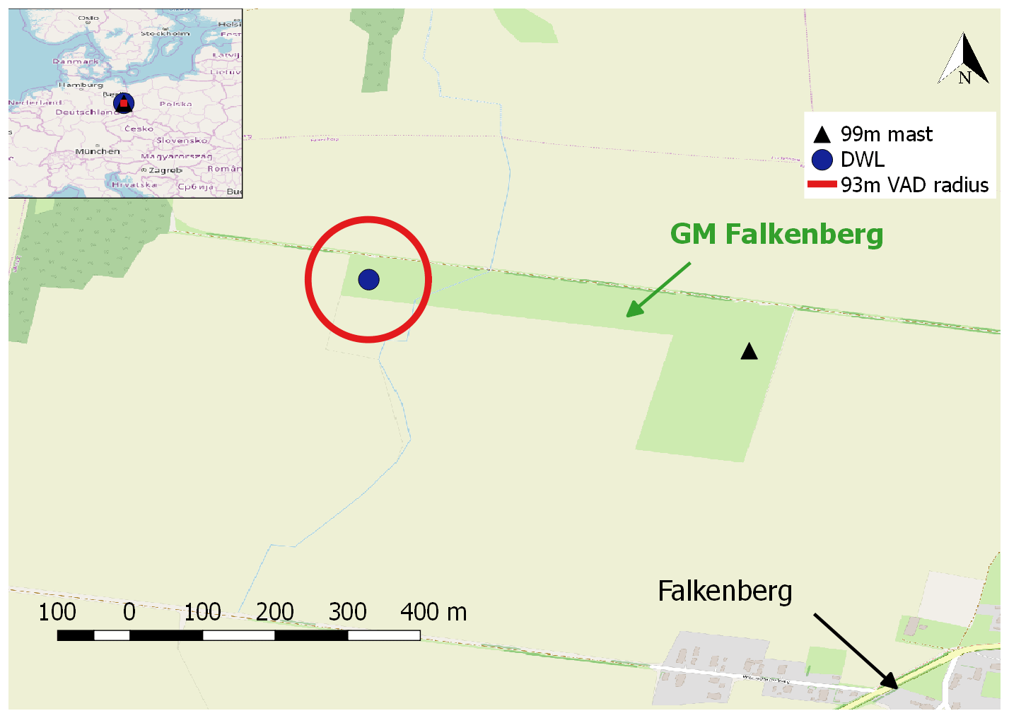
Figure 1Sketch of the measurement site at MOL-RAO, GM Falkenberg. Map data © OpenStreetMap contributors 2019. Distributed under a Creative Commons BY-SA License.
Since 2014, MOL-RAO has been using a DWL “Stream Line” (Halo Photonics Ltd.) for boundary layer measurements. From that time the device has been extensively tested with respect to its operational use for wind and turbulence measurements. This included, for instance, tests of the technical robustness and data availability under all weather conditions, but also tests of different scanning strategies and retrieval methods for the 3D wind vector and for the TKE. The position of the DWL during a measurement period from 2 through 30 April 2019 was at the western edge of the field site at about 500 m of distance from the 99 m tower. It should be noted that there is a small patch of forest about 300 m to the W-NW of the lidar site. During this period the system continuously performed VAD scans with an elevation angle of 35.3∘, which will be analyzed for turbulence retrievals in this study.
Continuous turbulence measurements (20 Hz sampling frequency) using a sonic anemometer of type USA-1 (METEK GmbH) are performed at the 50 and 90 m levels on the tower and have been used for validation purposes. The instruments are mounted at the tip of the booms pointing towards south.
2.2 The CoMet (CO2 and Methane) mission 2018
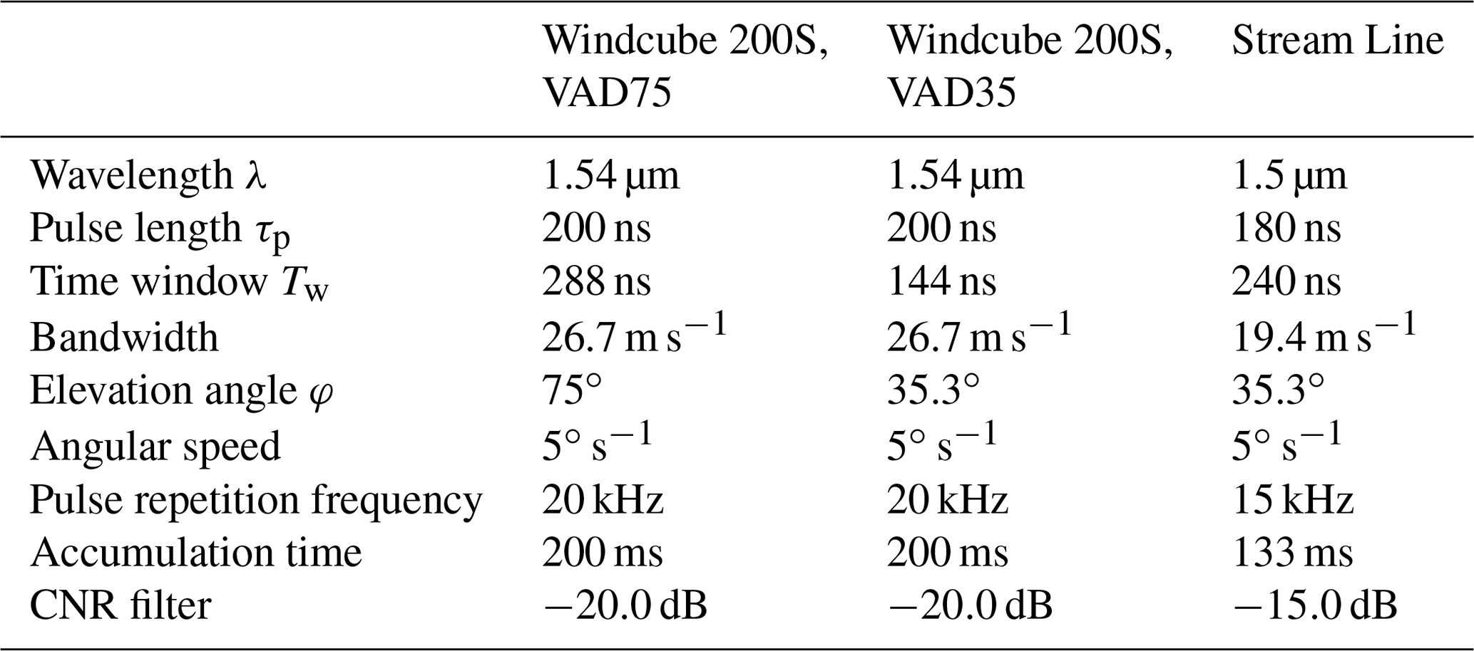
Within the scope of the CO2 and Methane (CoMet) mission that was conducted in spring 2018, three Doppler wind lidars of type Leosphere Windcube 200S (details see Table 1) were installed in Upper Silesia (Poland) with the purpose of providing spatially distributed wind and turbulence measurements in the ABL. CoMet aims at a better understanding of the budgets of the two most important anthropogenic greenhouse gases (GHGs), CO2 and CH4. For this purpose, the research aircraft HALO (high altitude and long range) was taking remote sensing and in situ measurements over large parts of the European continent. A dedicated area of high interest was the region of Upper Silesia, where large amounts of methane are known to be released due to the intensive coal extraction activities in the coal basin. During the CoMet campaign, the DLR Cessna Grand Caravan 208B (D-FDLR) aircraft was equipped with in situ instruments to measure greenhouse gases and thermodynamic variables.
Table 1Main technical specifications of the Doppler wind lidars.
The DWL measurements are particularly helpful to support the CoMet measurements by providing wind information that is essential to derive emission flux estimates from passive remote sensing (Luther et al., 2019) or in situ measurements of mass concentrations (Fiehn et al., 2020). The DWL wind information can also be used to validate modeled wind from the transport models for greenhouse gases. The lidars were remotely operated during the whole CoMet campaign period from 16 May to 17 June 2017 and were continuously measuring. The locations of the three lidars were planned to cover the whole region of interest and were finally chosen based on logistical constraints.
The lidars were operating in VAD modes with two different elevation angles. Since the focus for the CoMet campaign was on continuous wind profiling and a good height coverage was desired, the lidars were programmed to perform VADs with an elevation angle of 75∘ (see Table 1, VAD75) for a longer period, i.e., 24 scans (≈29 min), followed by only six scans (≈7 min) at a 35.3∘ elevation (VAD35) for turbulence retrievals.
As shown in Fig. 2, the three lidars were separated by several tens of kilometers and were located in different terrain types. While DWL no. 1 was in a mixed rural and urban area, DWL no. 2 was in a mostly forested environment, and DWL no. 3 was in close vicinity to the lake Goczałkowicki. The main wind direction during the campaign was from the east, with particularly strong winds during nighttime low-level jet (LLJ) events. In this study we analyze statistics of the whole campaign, as well as a case study on 5 June 2017, on which D-FDLR was performing long straight and level legs between 800 and 1600 m as indicated in the flight path in Fig. 2. Since the D-FDLR was focusing on GHG measurements at the hotspots of the Upper Silesian Coal Basin, there are no more straight and level flight paths that allow for turbulence retrieval. For this day, however, the research aircraft provides a unique possibility to validate lidar measurements with in situ measurements at higher altitudes that cannot be reached with sonic anemometers. The flow probe and inertial measurement unit on the D-FDLR are well-established instruments that allow for reliable measurements of the 3D wind vector and turbulence (Mallaun et al., 2015).
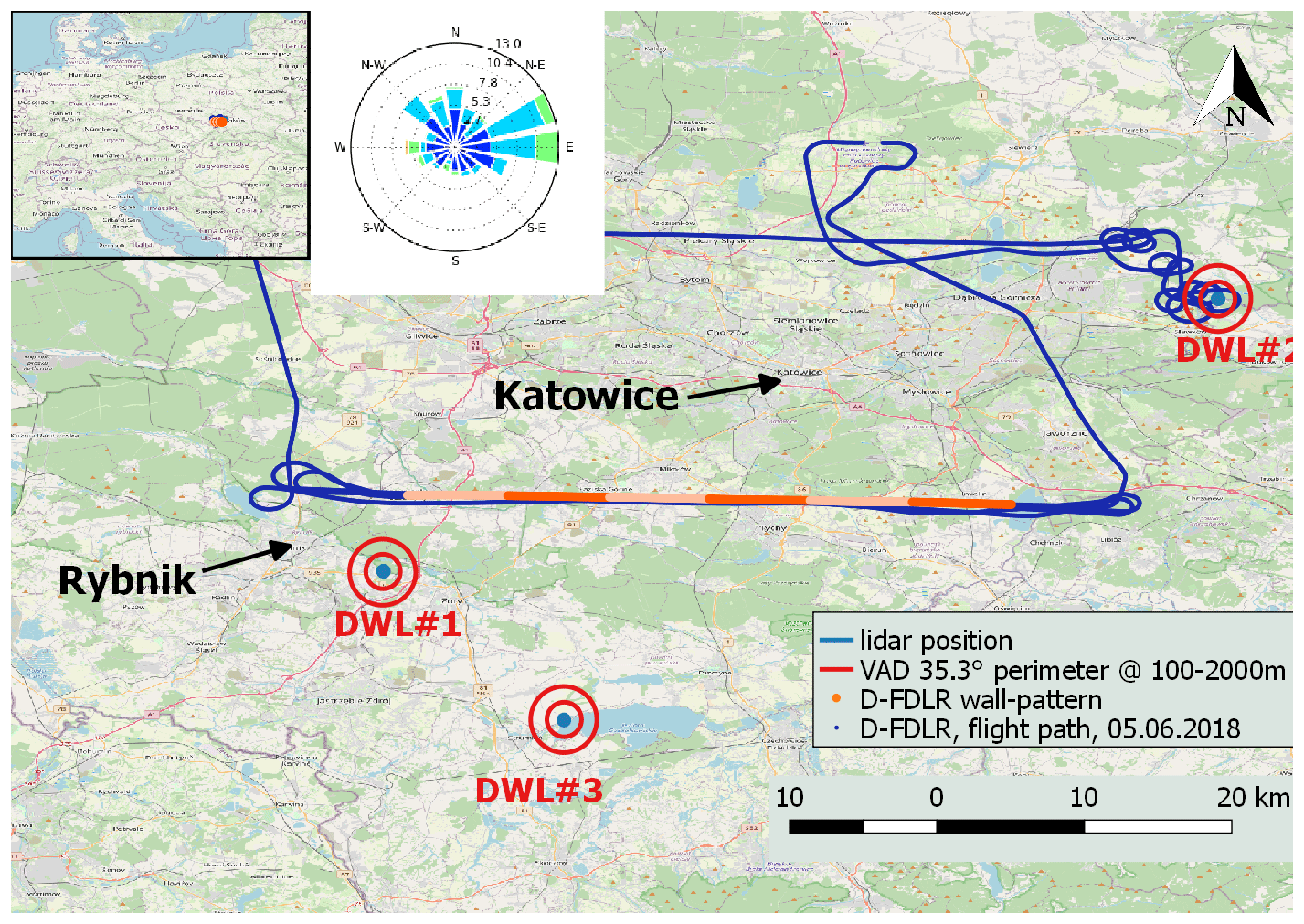
Figure 2Sketch of the measurement site in Upper Silesia. Red circles show the extent of the VAD scan at 35.3∘ for 100 and 2000 m at the respective lidar location. The orange line marks the flight path of D-FDLR on 5 June 2017. The different shades of orange are used to indicate a subdivision of the flight leg in shorter sub-legs. Map data © OpenStreetMap contributors 2019. Distributed under a Creative Commons BY-SA License.
3.1 Sonic anemometer turbulence measurements
From the sonic anemometers on the meteorological mast, TKE and the TKE dissipation rate are calculated. TKE is calculated from the sum of variances . The TKE dissipation rate ε is estimated through a fit of the theoretical longitudinal Kolmogorov structure function in the range τ1=0.1 s to τ2=2 s to the measured second-order structure function of horizontal velocity. Muñoz-Esparza et al. (2018) showed that the structure function method is more robust than estimates from spectra. For this study, in order to have the best possible comparison to the lidar measurements the values for ε are calculated for 30 min intervals. The geometry of the sonic anemometer setup disturbs the measurements for wind directions from 330 to 50∘ (see also Appendix D). Data for these wind directions are removed from the analysis.
3.2 VAD turbulence measurements
Methods to retrieve turbulence parameters from VAD scans are well-known and a variety of different methods exist. The method we refine in this study is based on the theory that was originally described by Eberhard et al. (1989) for lidar measurements. The variance of radial velocities depends on the range gate distance R, the azimuth angle θ, and the elevation angle φ. It is calculated from the measured radial velocities Vr:
From a partial Fourier decomposition (see Appendix A) and for the special case of φ=35.3∘, a simple equation for ETKE is derived:
In this equation, is the mean of the variance of radial velocities over all azimuth angles. In the following, we will refer to this method as E89 retrieval.
In order to retrieve estimations of the TKE dissipation rate ε from VAD scans, a similar approach to the method for sonic anemometers can be followed. A fit of the equation
to the azimuth structure function yields an estimate for ε according to Smalikho and Banakh (2017). In Eq. (4) Dr is the transverse structure function of radial velocities, CK the Kolmogorov constant, ψ the azimuth angle increment, and . We will refer to this method as S17A in the following.
Scanning with Doppler lidar in a classical VAD with continuous motion of the azimuth motor involves a volume averaging of radial velocities in the longitudinal (along the laser beam) and transverse (orthogonal to the beam) direction. The E89 and S17A methods do not consider this effect and will thus yield a systematic underestimation of TKE and ε. Smalikho and Banakh (2013) proposed a theory that considers the volume averaging and allows for the retrieval of ε from conical scans, independent of the elevation angle. In Smalikho and Banakh (2017), this method has been combined with the E89 method to yield TKE, ε, and the momentum fluxes. It is based on the decomposition of radial velocity variance into its subcomponents, i.e.,
where is the lidar-measured variance, is the lidar-measured variance without instrumental error , and is the turbulent broadening of the lidar measurement. In Smalikho and Banakh (2017), all of these variances and structure functions are calculated for single azimuth angles and then averaged. We describe in Sect. 3.2.1 why we use the total variances and structure functions of all radial velocities.
The measured azimuth structure function Da(ψl) is a function of the separation angle ψl, where l is the index of the discrete separation angle of the scan. It can be decomposed into the lidar-measured structure function DL(ψl) and the instrumental error :
Combining Eq. (7) with Eq. (9) yields
It shows that since the instrumental error is assumed to be a constant offset of azimuth structure function Da(ψl) and the lidar measurement DL(ψl), l can be chosen arbitrarily here. It is set to l=1 because potential random errors like nonstationary flow will be smaller for small separation angles. Using Eqs. (3) and (21) (see Sect. 3.2.1), TKE can be redefined as a function of the measured line-of-sight variances , the measured lidar azimuth structure function of radial velocities DL(ψ1), and a residual term G, which includes the two unknowns, and Da(ψ1):
In Banakh and Smalikho (2013), a relationship between the two unknowns and the TKE dissipation rate is theoretically derived from the two-dimensional Kolmogorov–Obukhov spectrum as
where F(Δy) and A(lΔy) are model functions that include the lidar filter functions (see Appendix B). The lidar filter functions in the longitudinal direction depend on the pulse width of the laser beam Δp and the time window Tw of the data acquisition. The transverse filter function is defined by Δy=RΔθcos φ, which is the distance the lidar beam moves along the cone during one accumulation period. The parameters for the lidars in this study are provided in Table 1 and are calculated from information given by the manufacturer for the specific lidar type. Hence, G depends on the turbulence dissipation rate ε:
Using Eqs. (14) and (9), ε can be retrieved from Da(ψl)−Da(ψ1):
This equation does not depend on the elevation angle so that the method allows for the retrieval of ε from VAD scans with elevation angles different from 35.3∘ as well. Figure 3 gives an example of the different structure functions that are calculated in this method (i.e., DL, Da, and A) and also gives a comparison to the structure function Ds as calculated from sonic anemometer measurements. Smalikho and Banakh (2017) found a separation angle of lΔθ=9∘ to be an appropriate value for ABL measurements. In this study, all VAD scans are performed with a resolution of Δθ=1∘ so that l=9. In Fig. 3 the range that is thus used for the structure function fit is indicated by the bold black line.
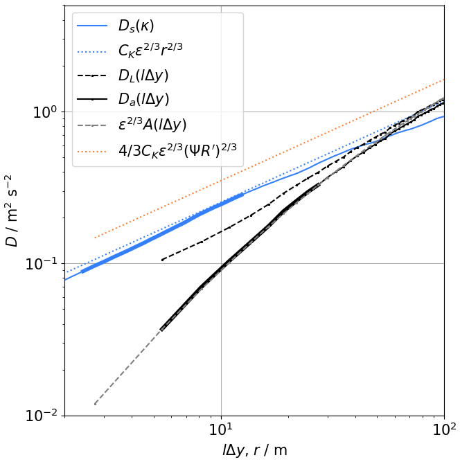
Figure 3Example of the structure functions of sonic anemometer (blue) and lidar (grey) at 90 m of height on 4 April 2019, 12:00–12:30 UTC. The dashed black line shows the measured lidar structure function DL, and the solid black line Da is corrected for the systematic error σe (see Eq. 9). The grey dashed line gives the model structure function A, and the dotted lines indicate the reconstructed inertial subrange for the calculated values of ε. The parts with bold lines are those ranges that are used for the structure function fits.
The retrieval method for ε using Eq. (16) and TKE using Eq. (11) will be referred to as S17 in the following.
3.2.1 Modifications for a small number of scans
The VAD at φ=35.3∘ during the CoMet campaign was not run continuously, but only six individual scans were performed successively before switching back to the VAD at φ=75∘ as described in Sect. 2.2. This means that only six data points are available to calculate the variance and mean of the radial velocities at each azimuth angle, which cannot be considered a solid statistic. We introduce two modifications of data processing to overcome this problem that are based on the assumptions of stationary and homogeneous turbulence.
Practical implementation of the ensemble average
In Eq. (2), can be calculated as the arithmetic mean of radial velocities at specific azimuth angles:
where N is the number of scans. Instead of this approach, we suggest using the reconstructed radial velocity from the retrieved wind field over all individual scans as the expected value in the variance calculation. For the retrieval of the three wind components (, , ), filtered sine-wave fitting (FSWF) is applied (Smalikho, 2003). The reconstructed radial velocities are then used as the expected value in the variance calculation:
With this approach, all measurement points in the VAD with the same elevation angle are used to obtain the expected value 〈Vr〉, and thus a better statistical significance is achieved. This method has also been proposed in Smalikho and Banakh (2017) as a practical implementation of Eq. (2).
Averaging of variances
In Smalikho and Banakh (2017), the variances of the lidar measurements are defined as the average of variances at individual azimuth angles:
The variances are the variances of a subsample of the radial velocities of the VAD (i.e., those at a specific azimuth angle θm). We use a simple relation between the variances of subsamples and the total variance of a dataset (see Appendix C). Applying this to the radial velocity variances yields
where k is the number of samples at each azimuthal angle, g is the number of subsamples, and n is the number of total samples in the dataset (n=gk). Since the mean of the radial velocity fluctuations is zero by definition, Eq. (21) becomes
3.2.2 Filtering of bad estimates
Improvements of turbulence estimates in low signal conditions can be achieved by filtering bad estimates as described in Stephan et al. (2018). This approach is not based on the calculation of the azimuth structure function from measured radial velocities but uses probability density functions (PDFs) and their corresponding standard deviations. The model PDF is defined as a Gaussian function with a filter term P:
where P is the probability of bad estimates of x, σ is the standard deviation of the PDF, and Bv is the velocity bandwidth of the lidar. Equation (23) is fit to the observed distributions of vr(R,θ), , and by adjusting the corresponding values σ1, σ2, and σ3 and the probability of bad estimates P1, P2, and P3. The values of σi are used as the first guess of the standard deviation of the distributions. However, since the PDFs cannot be assumed to be Gaussian in atmospheric turbulence, the standard deviations are finally calculated as the integral over the measured PDFs in the range ±3.5σ according to Stephan et al. (2018).
Replacing with , DL(ψ1) with , and DL(ψl) with in Eqs. (11) and (16) yields
and
As suggested in Stephan et al. (2018), Eqs. (24) and (25) are only used if P>0. We also introduced a quality control to discard any measurements with P>0.5 for best results. In practice, this method will thus only be applied in some conditions when the signal is weak and can extend the range of vertical profiles to some degree.
3.2.3 Correction for advection
The azimuth structure function and the volume-average filter are distorted by advection through a modification of Δy. The effect is illustrated in Fig. 4. It shows that the distance between measurement points in a flow-fixed coordinate system is unequally spaced and on average larger than in the earth-fixed coordinate system. We propose a simplified correction. When advection is not considered, the spacing between samples is given by
An estimate of the mean spacing can be obtained from
where . We propose a simplified correction in which
where

Figure 4Sketch of the measurement points of a VAD scan in an earth-fixed versus a flow-fixed coordinate system.
Here, R is the range gate distance, φ is the elevation angle, xi and yi are the measurement point locations, Ψ is wind direction, U is wind speed, and Δt is the accumulation time of the lidar. The terms cos ΨUΔt and sin ΨUΔt describe the effect of advection on the measurement location in the x and y direction, respectively. Using the corrected measurement location displacements dxc,i and dxc,i, we can calculate a corrected mean transverse sensing volume Δyc. This method does not account for the unequal spacing but corrects the average separation of data points, which is particularly important for the statistical evaluation of turbulence.
The effects of advection on the turbulence estimation are largest in the lowest levels of the VAD scans because Δy is small compared to UΔt in this case. The retrieval method including filtering for bad estimates and the advection correction is referred to as W20 in the following.
3.2.4 Quality control filters
In order to fulfill the assumptions that are made with regards to the turbulence model and the turbulence retrieval method, the data are filtered according to the criteria given in Smalikho and Banakh (2017):
For the purpose of evaluating the methods in a broad range, we set mild criteria for Eqs. (31) and (33) using
and
Equations (31) and (32) are criteria that require the integral length scale Lv to be larger than the sensing volume of the lidar in the transversal (Δy) and longitudinal (Δz) direction. Unfortunately, there is no independent measurement of Lv at all heights of the VAD scan so that it is derived from the lidar measurement itself as (Smalikho and Banakh, 2017).
The filter criteria in Eq. (33) provide a filter for conditions with significant advection, which distorts the measured structure functions and is only applied if the method described in Sect. 3.2.3 is not used.
Except for the retrieval method W20, which uses the filtering of bad estimates, we set fixed CNR filter thresholds adapted to the lidar type. Since the turbulence retrievals are very sensitive to bad estimates, we set the CNR thresholds to conservative values that are given in Table 1.
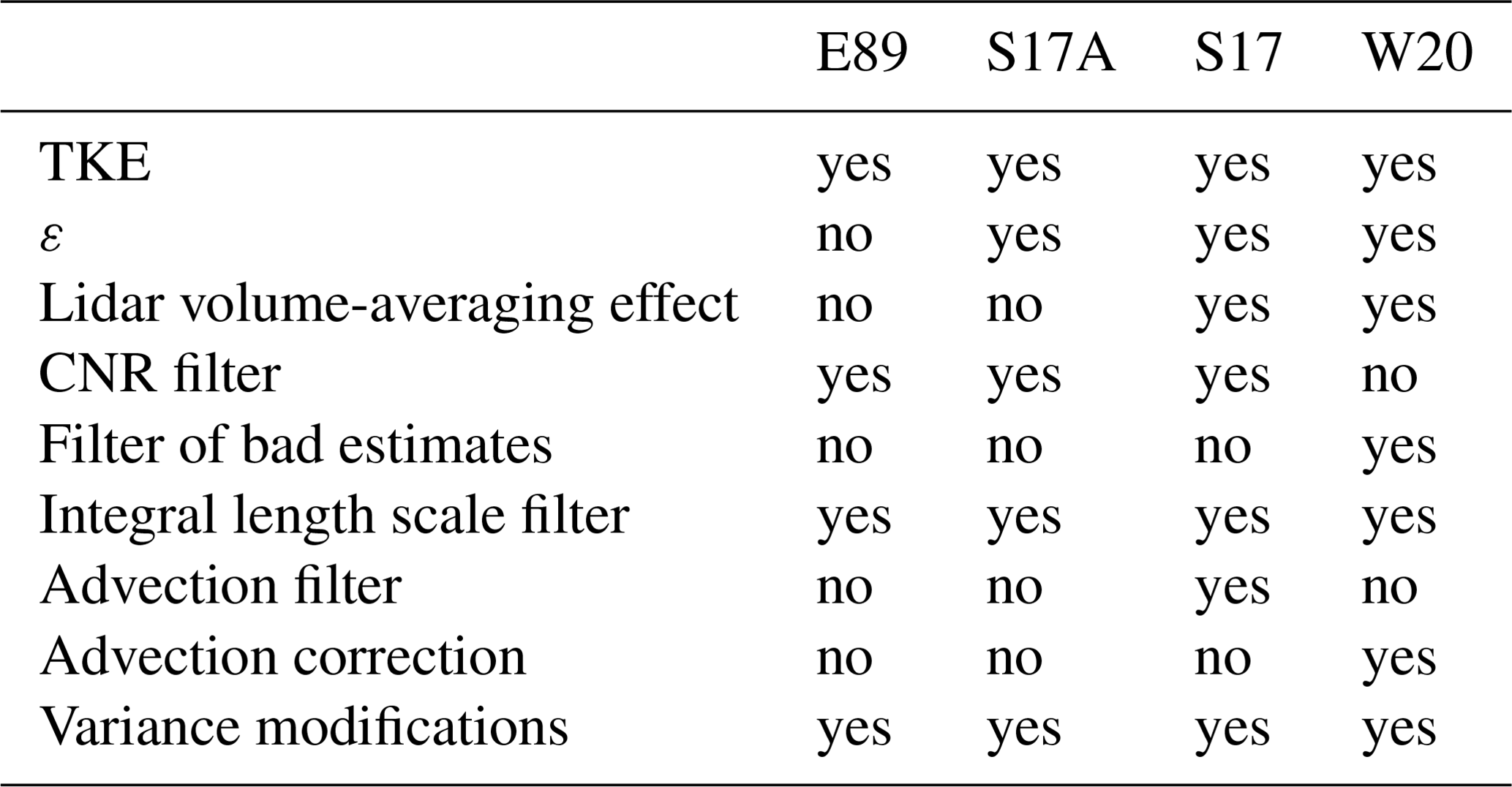
An overview of all retrieval methods and their characteristics and filters that are applied is given in Table 2.
Table 2Overview of turbulence retrieval methods and the applied filters and methods.
3.3 Turbulence estimation from airborne data
The estimation of turbulence parameters from the wind measurement system on the DLR Cessna Grand Caravan 208B (Mallaun et al., 2015) is done very similarly to the in situ estimations from the sonic anemometer. TKE is calculated from the sum of variances as described in Sect. 3.1. The dissipation rate is also calculated from the second-order structure function but with different bounds for the time lag. For the flight data we use τ1=0.2 s and τ2=2 s, corresponding to approximately 13–130 m lag at 65 m s−1 mean airspeed.
To evaluate the heterogeneity of turbulence due to changing land use along the flight legs of more than 50 km length, we divided the legs into sub-legs of 6.5 km (i.e., 100 s averaging time) and calculated turbulence for each leg individually. The location of the legs and the sub-legs is shown in Fig. 2.
4.1 Comparison to sonic anemometer
The best possible validation of the methods introduced in Sect. 3 can be performed with the lidar in close proximity to the meteorological mast such as at the measurement site at MOL-RAO. The sonic anemometers at 50 and 90 m on the mast almost coincide with the measurement levels of the lidar at 52 and 93.6 m, respectively. Since the VAD retrieval with an elevation angle of 35.3∘ yields TKE and its dissipation rate, both turbulence parameters can be compared to values obtained from the sonic anemometers. In this section we will evaluate the methods described in Sect. 3.2, in particular the validity of the assumptions made in Sect. 3.2.1 and the efficiency of the advection correction described in Sect. 3.2.3.
4.1.1 Validation of modified variance
In Sect. 3.2.1 we introduced two modifications to the calculation of the averaged lidar radial velocity variances. These changes are especially necessary if a low number of VAD scans is used for turbulence retrieval. In the MOL-RAO experiment, VAD scans are run continuously with φ=35.3∘ so that the modifications can be tested against the original version of the retrieval method. The sonic anemometer at 90 m on the meteorological mast serves as an independent validation measurement. Figure 5a shows a time series of the two methods and the sonic anemometer in a time period in which all systems were providing good data almost without interruption (22–29 April 2019). The lidar retrieval with both variance methods follows the sonic anemometer TKE estimation very well through the diurnal cycles, with some occasional overestimation that will be discussed in Sect. 4.1.2. Figure 5b gives the difference (ΔTKE) between the azimuth average and total average to show that it is typically below 0.5 m2 s−2 except for some periods with strong gradients in TKE. Figure 5c shows the scatterplot that directly compares the S17 retrieval calculated with azimuth-averaged variances to the S17 retrieval using total variances. There is a higher estimation of TKE in the total variance method, which increases with TKE. We cannot fully explain this effect at this point, but it might be due to the small-scale turbulence that cannot be resolved with the 72 s sampling rate of radial velocities at individual azimuth angles. It is small enough to be neglected for further analysis.
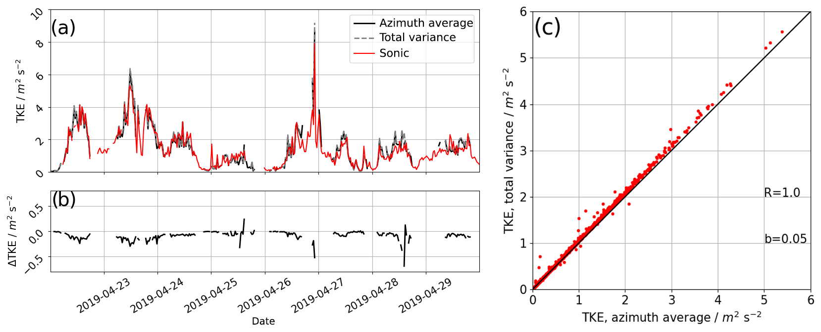
Figure 5Time series of TKE from lidar retrievals compared to a sonic anemometer at 90 m above ground level (a), the difference between the lidar retrieval with averaged variances (Eq. 20) at specific azimuth angles θ to the modified total variance method (Eq. 21) (b), and the scatterplot for the whole experimental period (c).
4.1.2 Comparison of lidar retrievals
The MOL-RAO dataset allows us to compare the retrievals without consideration of lidar volume averaging (E89 and S17A) to the S17 retrieval and its modified version W20 introduced in this study. For this purpose, the individual retrieval results are compared to the sonic anemometer estimates of TKE and its dissipation rate ε. Figure 6 shows the scatterplots for TKE at the two measurement levels. For each method, the coefficient of determination of the linear regression between the sonic measurement and lidar retrieval is given, as is a bias that is calculated as for TKE and for ε. We find that with the E89 method, TKE is systematically underestimated, as expected. In contrast to that, the S17 method yields slightly overestimated TKE values if no advection filter is applied (light red dots) but good agreement with the sonic anemometer in the absence of advection (red dots). The overestimation of TKE is larger for the lower level at 50 m compared to the 90 m level, which we attribute to the smaller averaging volume Δy. Our refined version of the retrieval including the advection correction improves the results slightly, especially for the high-turbulence cases (corresponding to high wind speeds) at the 50 m level, as the scatterplots show. Figure 7 gives the scatterplot comparison of ε retrieval from S17A, S17, and W20 with the sonic anemometer. E89 does not provide an estimate for ε. Even more clearly than for TKE, the underestimation of the method without consideration of lidar volume averaging (S17A) is found. Also, a now positive bias of b=0.09 m2 s−2 for lidar estimates with the S17 method at the 50 m level is reduced with the advection correction to b=0.06 m2 s−2. It is evident from the ε estimates that all lidar retrievals underestimate turbulence significantly compared to the sonic anemometer in the low-turbulence regimes, in particular for values smaller than m2 s−3, which is why these values have been excluded for the estimation of biases (grey dots).

Figure 6Scatterplot of lidar TKE retrieval against sonic anemometer TKE at the 50 m level (a–c) and 90 m level (d–f). E89 retrieval is shown in panels (a) and (d), S17 retrieval in panels (b) and (e), and W20 retrieval in panels (c) and (f). The light red dots in panels (b) and (e) show all TKE estimates with no filter for advection; the dark red dots have the advection filter applied.
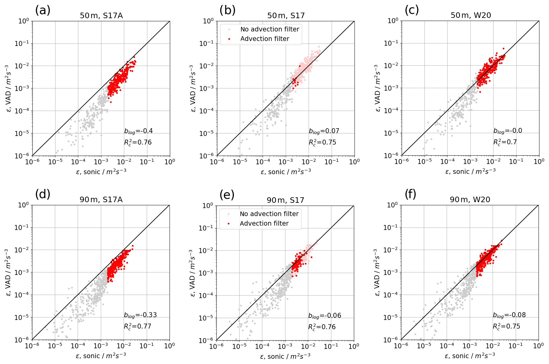
Figure 7Scatterplot of lidar dissipation rate retrieval against the sonic anemometer dissipation rate. The light red dots in panels (b) and (e) show the results with no advection filter. The light grey dots are all estimates below m2 s−3. Grey dots are not used for the calculation of R and blog.
4.1.3 Evaluation of advection error
To evaluate the error that is caused by advection in the S17 retrieval, all data that were collected at MOL-RAO were binned into wind speeds with a bin width of 1 m s−1. The mean absolute error between the lidar retrievals and the sonic anemometers at the respective level is calculated and shown in Fig. 8 for TKE and ε. Although the averaged errors of TKE are small in general, it shows that the W20 method does reduce the error in comparison to the S17 method at the 50 m level. The error for ε at the 50 m level increases with wind speed but less for the W20 method. Hardly any improvement is found for the already small errors of TKE and ε at 90 m.

Figure 8Difference of the lidar retrieval of TKE (a) and the TKE dissipation rate (b) compared to the sonic anemometer as a function of wind speed.
4.2 Comparison of elevation angles
VAD scans with 35.3∘ allow for the retrieval of TKE and momentum fluxes using the methods described in Sect. 3. The disadvantage compared to VAD scans with larger elevation angles is that at the same range of the lidar line-of-sight measurement, lower altitudes are reached. If the limit of range is not given by the ABL height in any case, this can lead to significantly lower data availability at the ABL top. Another advantage of greater elevation angles is that the horizontal area that is covered with the VAD, and thus the footprint of the measurement, is much smaller than with low elevation angles. From the theory derived in Sect. 3.1, we see that the dissipation rate retrieval does not depend on the elevation angle and can thus also be obtained from VAD scans with a 75∘ elevation angle if the assumptions of isotropy and homogeneity hold. However, since the VAD at 75∘ has the more narrow cone, the separation distances Δy at respective measurement heights are smaller, and thus the sensitivity to advection errors is expected to be larger. The measurements with two different elevation angles during the CoMet campaign allow us to compare dissipation rate retrievals for both kinds of VAD scans with the restriction that they are not simultaneous but sequential.
Figure 9 shows the comparison of both types of VADs in scatterplots of three measurement heights for the whole campaign period and DWL no. 1. In general, a large scatter is found between the two types of VAD that can be attributed to the different measurement times, different footprint, and heterogeneous terrain. Applying a filter for significant advection as described in Sect. 3.2.4 removes most of the measurement points at the 100 m level in the 75∘ VAD. Without the filter (grey and red points), large systematic overestimation against the VAD at 35.3∘ is found, which can still be seen at 500 m but is no longer found at 1000 m. With the advection correction of W20, the systematic error is reduced, but the random errors remain.
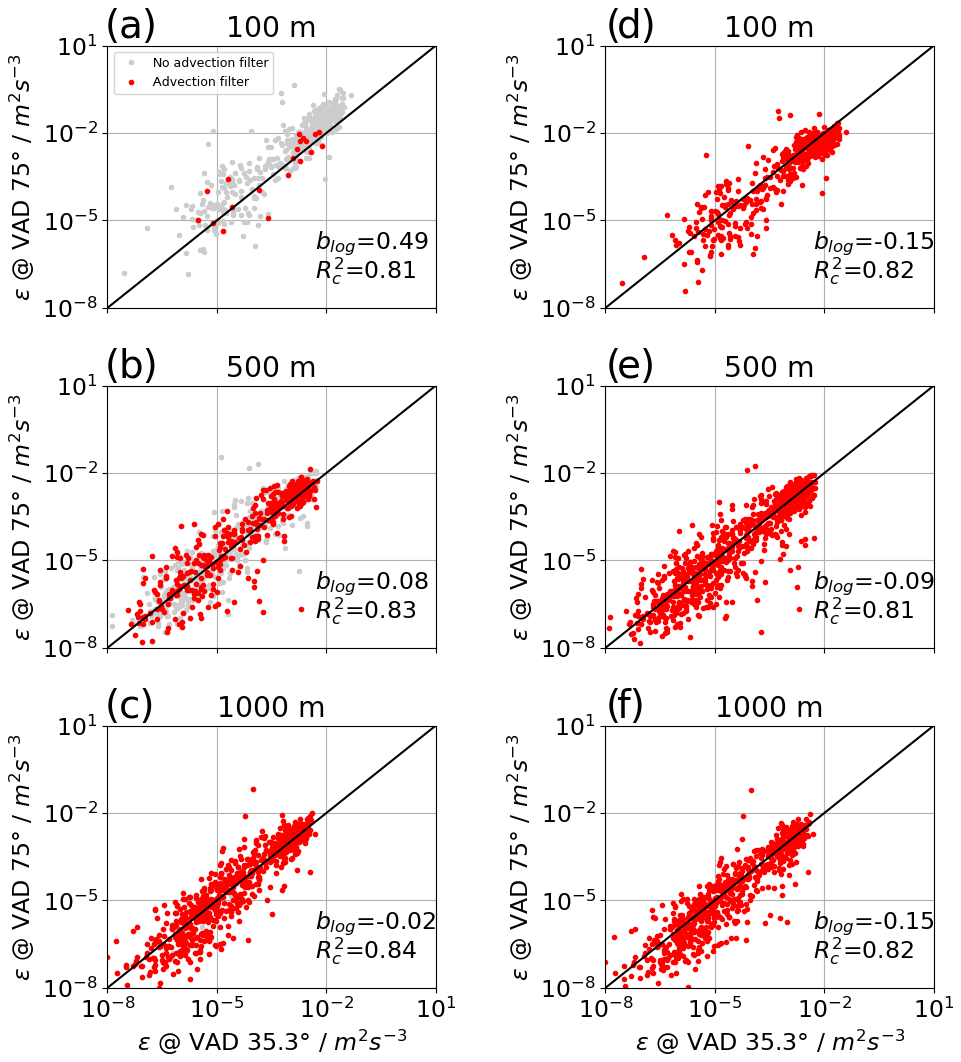
Figure 9Scatterplot of lidar dissipation rate retrieval from VAD scans with a 75∘ elevation angle versus 35.3∘. On the left, retrievals without advection correction are shown for three different levels at (a) 100 m, (b) 500 m, and (c) 1000 m. On the right, the corresponding scatterplots with advection correction are presented (d–f).
As for the comparison with the sonic anemometer, we evaluate the error as a function of wind speed by binning the data in wind speeds between 0 and 10 m s−1 (see Fig. 10). A clear trend is found for the 100 m level, which can be significantly reduced with the W20 method. A very small difference between the two elevation angles at the 500 m level is only reduced very little in the W20 method.

Figure 10Difference of lidar ε retrievals for both kinds of VAD as a function of wind speed.
4.3 Comparison to D-FDLR
During CoMet, no meteorological tower with sonic anemometers at levels that could be compared to the Doppler lidars was available. Instead, the aircraft D-FDLR was operating with a turbulence probe and provided in situ turbulence data. On 5 June 2018, the aircraft was flying a so-called “wall” pattern, with long, straight, and level legs at five altitudes (800, 1000, 1100, 1300, and 1600 m). At least the lowest three levels of this flight allow for a comparison to the measurement levels of the top levels of lidar measurements on this day. Figure 11 shows the measured TKE of D-FDLR at the five flight levels. Only at the lowest two light levels (i.e., 800 and 1000 m) is significant turbulence measured, with strong variations along the flight path.

Figure 11D-FDLR TKE measurements at five flight levels. Map data © OpenStreetMap contributors 2019. Distributed under a Creative Commons BY-SA License.
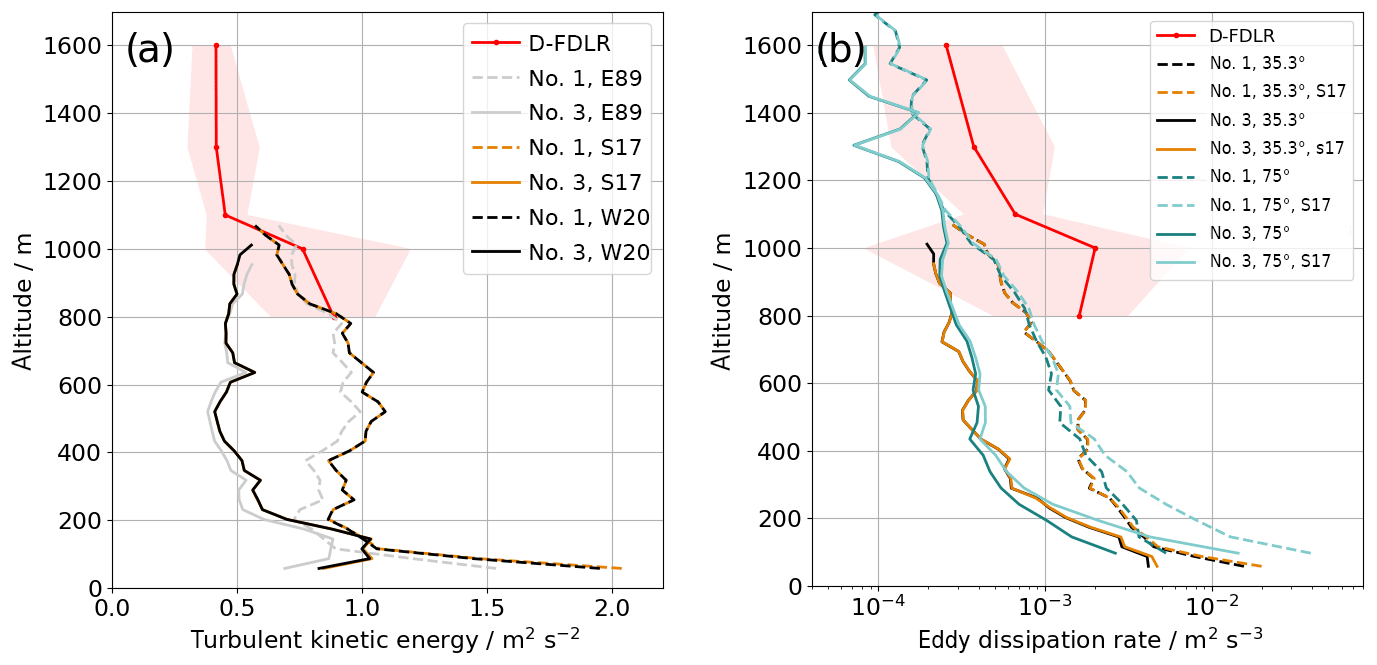
Figure 12 shows the measurements from D-FDLR and the lidars DWL no. 1 and DWL no. 3 that were taken between 14:00 and 15:30 UTC as vertical profiles. The solid red line gives the average of all sub-legs along the 50 km flight of D-FDLR, and the shaded areas give the range between the minimum and the maximum at each height. It nicely shows how the measurements of turbulence at the DWL no. 3 site are significantly lower than at DWL no. 1, which we attribute to the lake fetch. The D-FDLR measurements of TKE almost match the DWL no. 1 site and are all higher than at the DWL no. 3 site, which makes sense given the environmental conditions of heterogeneous land use. Figure 12a also gives a comparison between E89, S17, and W20 estimates from the same dataset. Here, it shows that the difference between S17 and W20 only occurs at the very lowest level, but the underestimation of the E89 method is found up to 750 m. In dissipation rate estimates, the DWL no. 1 measurements are at the low end of the range that was measured with D-FDLR, and the lake-site measurements are even smaller. The estimates from 35.3∘ scans and 75∘ scans agree very well, especially at the higher levels, which shows that the assumption of isotropy and homogeneity seems to hold. The presumed underestimation of the ε of lidar retrievals compared to in situ measurements at absolute values of 10−3 m2 s−3 is consistent with what was found for the comparison to sonic anemometer measurements. This single case of airborne measurements compared to lidar retrievals at higher altitudes cannot, however, provide any statistical validation.
Figure 13 shows measurements of ε retrieved with the W20 method for the VAD scans with 75∘ elevation and all three lidars. It shows that the growth of the boundary layer with its increased turbulence can be nicely captured by the lidars. There are some differences between the three locations, especially lower turbulence close to the ground at the DWL no. 3 location and a higher boundary layer at the DWL no. 2 location. More studies will be necessary in the future, analyzing the data from the whole campaign, to improve the understanding of land–atmosphere interaction in this case.
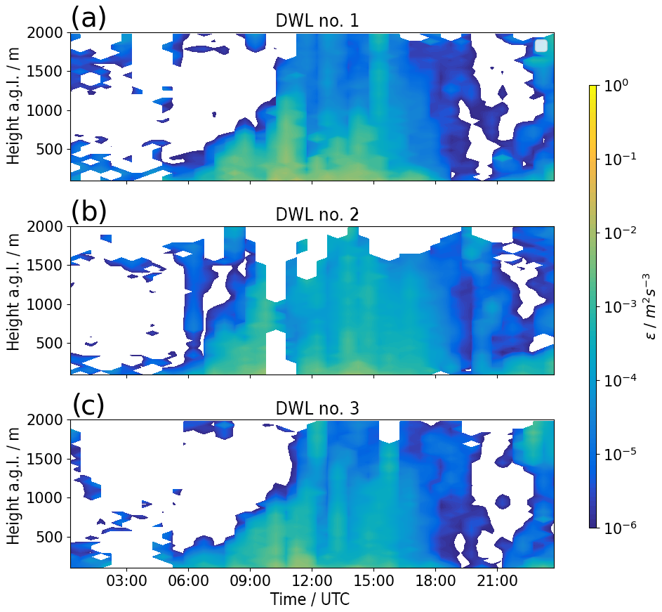
Figure 13Diurnal cycle of the TKE dissipation rate on 5 June 2018 at the three lidar locations calculated with the W20 method.
In this study, we used four different methods to retrieve turbulence parameters from the same data obtained through lidar VAD scans. The MOL-RAO experiment allowed us to investigate and validate the methods with a database of 30 d containing a broad variety of atmospheric conditions, with wind speeds of 0.12 m s−1 and TKE of 0.5 m2 s−2. This goes beyond the short-term studies of only a few days and specific atmospheric conditions investigated by Smalikho and Banakh (2017). Furthermore, two sonic anemometers allowed us to investigate the dependence of the retrieval on the measurement height. The experiment shows that methods that do not account for the lidar volume-averaging effect underestimate TKE and its dissipation rate compared to sonic anemometers at 50 and 90 m. The S17 method handles this problem but introduces an overestimation in our dataset. Parts of this overestimation can be attributed to advection, which distorts the retrieval of the azimuth structure function and the transverse filter function in the lidar model. The advection effects are relevant at the lowest measurement heights at which the spatial separation of lidar beams along the VAD cone Δy is small. This effect is stronger than increasing wind speeds at higher altitudes in our observations. We propose a correction for this issue and show here that our method reduces systematic errors compared to the sonic anemometers at the 50 m level. To confirm that advection is the reason for this improvement we show that the bias increases with wind speed. With all retrievals, dissipation rates with values smaller than 10−3 m2 s−3 are underestimated by the lidars, likely because the small-scale fluctuations that are carrying much of the energy in these cases can no longer be resolved. A remaining piece of uncertainty is represented by the lidar parameters Δp and Tw, which are given by the manufacturer for the lidar type but could potentially differ for individual lidars. Exact knowledge about these parameters could reduce the uncertainty of the model functions F and A (see Appendix B) and thus improve the corrections of the volume-averaging effects. It is conceivable that the observed overestimation of S17-based (and W20-based) TKE can also partly be attributed to these uncertainties.
The aircraft measurements that were carried out during the CoMet campaign were used to show the agreement of the lidar retrievals with in situ measurements at higher altitudes. It is the first time that these lidar measurements have been compared to in situ aircraft data. Unfortunately, only measurements for a single day allowed for a comparison, and the spatial separation of the measurements introduces additional uncertainty. It was found that TKE estimates from lidar and aircraft compare rather well, but the small values of dissipation rates at these heights are underestimated by the lidar to a similar order of magnitude as for low-turbulence conditions in the sonic anemometer comparison. Dedicated experiments will be necessary in the future to provide more comprehensive validation datasets for turbulence retrievals with lidar VAD scans. Given the larger separation distances Δy of the lidar beams at higher altitudes, the assumption that lΔy≪Lv is more likely to be violated. Airborne in situ measurements are the best way to validate the assumptions and the lidar retrievals in these cases.
The CoMet dataset was also used to show that VAD scans with a larger elevation angle (here: 75∘) can be used to retrieve the TKE dissipation rate with the same method as for VAD scans with 35.3∘, and the results are comparable. For these narrow VAD cone scans, we showed that the advection correction is much more important than for lower elevation angles, and strong overestimation of ε can occur in conditions with high wind speeds if it is not applied. The distribution of three lidars in Upper Silesia in areas with different land use shows the variability of turbulence and boundary layer flow in this area. VAD scans with different elevation angles have recently been used to describe the anisotropy of turbulence in a stable boundary layer (Banakh and Smalikho, 2019) and can potentially help to analyze horizontal heterogeneity and its impact on the calculation of area-averaged fluxes in the future.
Eberhard et al. (1989) show that radial velocity variance can be decomposed into the components u, v, and w of the meteorological wind vector:
A partial decomposition of Eq. (A1) yields the following.
These equations provide the basis for the retrieval of TKE and momentum fluxes from lidar VAD measurements.
Theoretical models for the spectral broadening of lidar measurements (F(Δy)) and the structure function (A(lΔy)) are derived in Banakh and Smalikho (2013) from the two-dimensional Kolmogorov spectrum for lidar measurements of turbulence.
Here, H∥ is the longitudinal and H⟂ the transverse filter function of lidar measurements in the VAD scan:
where Δp is derived from the FWHM pulse width τp, ΔR from the time window Tw, and Δy from the VAD azimuth increment Δθ.
For statistically independent subsamples Xj with size kj, the total variance of the dataset can be derived as follows:
where j is the index of the subsample and i the index of the element in the subsample.
Here, . Eventually, for equally sized subsamples one obtains the following.
The FSWF retrieval (Smalikho, 2003) is used to obtain the three-dimensional wind vector from the lidar VAD scans. The results of the retrieval are compared to the sonic anemometers at 50 and 90 m and shown in Fig. D1. To show the distortion of the mast, no data have been removed in the retrieval of wind speed and wind direction for this figure.
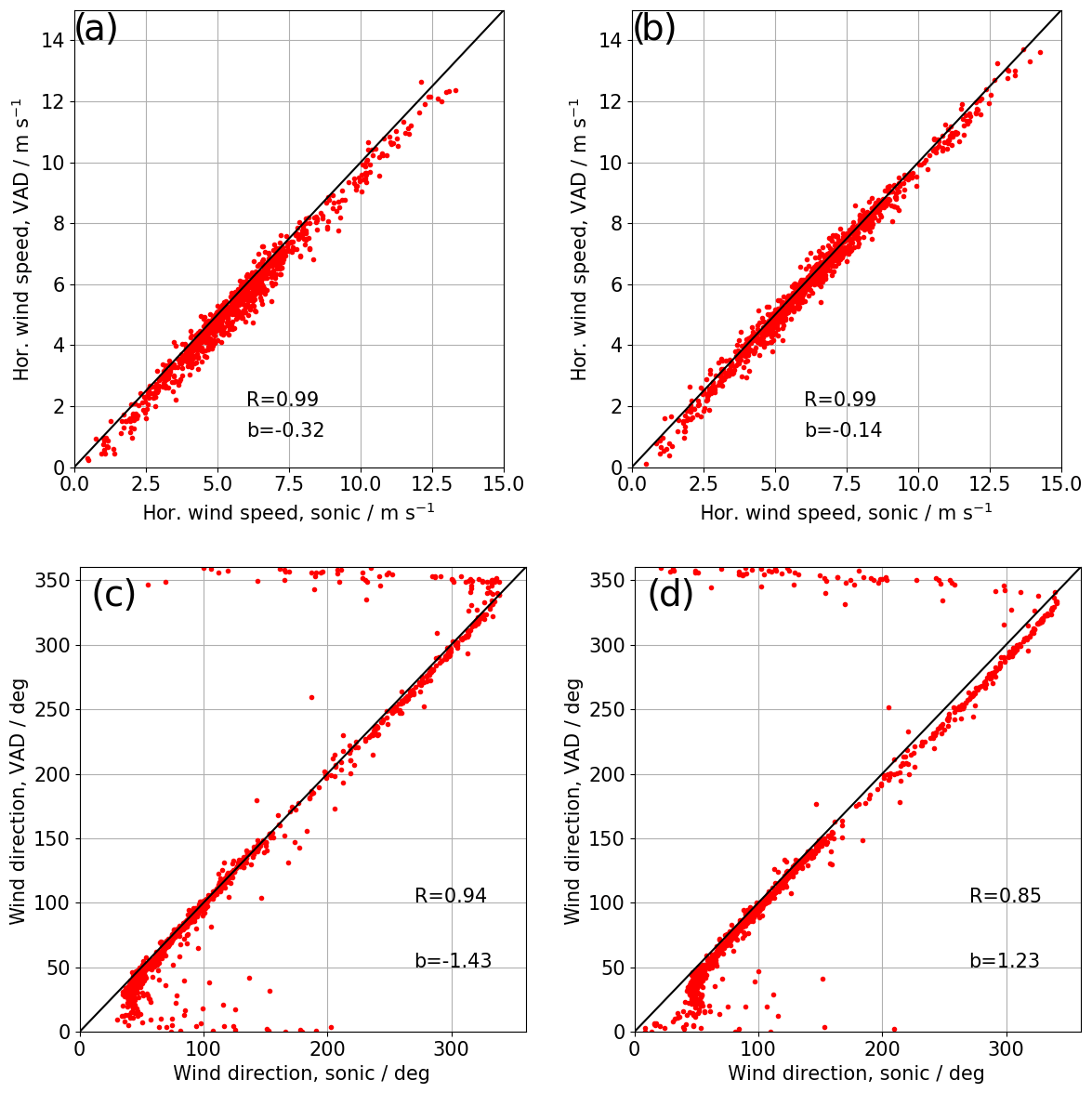
Figure D1Scatterplot of horizontal wind speed (a, b) and wind direction (c, d) retrieved from lidar measurements compared to sonic anemometer measurements at 50 m (a, c) and 90 m (b, d).
| λ | laser wavelength |
| τp | lidar pulse length (full-width at half-maximum, FWHM) |
| Tw | lidar time window |
| φ | elevation angle |
| θ | azimuth angle |
| u | wind component towards east |
| v | wind component towards north |
| w | upward wind component |
| u-wind component variance | |
| v-wind component variance | |
| w-wind component variance | |
| τi | time separation |
| Vr | radial wind component |
| vr | radial wind component difference from mean |
| radial wind component variance | |
| R | range gate distance |
| ETKE | turbulence kinetic energy |
| ε | TKE dissipation rate |
| CK | Kolmogorov constant |
| ψ | azimuth angle increment |
| κ | wave number |
| r | separation distance |
| variance of lidar measurements | |
| lidar instrumental noise | |
| variance of lidar measurements without instrumental noise | |
| turbulent broadening of the Doppler spectrum | |
| ΔR | distance between neighboring range gate centers |
| Dr | azimuth structure function |
| Ds | longitudinal structure function measured by sonic anemometer |
| DL | lidar measurement of azimuth structure function |
| Da | |
| A | theoretical model for azimuth structure function |
| F | theoretical model for turbulent broadening of the Doppler spectrum |
| Δy | distance of lidar beam movement during one accumulation period |
| Δyc | modified Δy for advection |
| pM | model PDF |
| P | probability of bad estimates |
| Lv | integral length scale |
| ωs | angular velocity of VAD scan |
| Ψ | wind direction |
| U | horizontal wind speed |
| Δt | accumulation time |
| Rc | linear regression correlation coefficient |
| b | measurement bias |
| H∥ | longitudinal low-pass filter function for lidar measurement |
| H⟂ | transversal low-pass filter function for lidar measurement |
The data are available from the author upon request.
NW, EP, AR, and CM helped design and carry out the field measurements. CM provided processed data from the D-FDLR aircraft turbulence probe. NW analyzed the data from the sonic anemometers, the profiling lidars, and the D-FDLR. NW wrote the paper, with significant contributions from EP. All the coauthors contributed to refining the paper text.
The authors declare that they have no conflict of interest.
This article is part of the special issue “CoMet: a mission to improve our understanding and to better quantify the carbon dioxide and methane cycles”. It is not associated with a conference.
We want to thank Jarosław Nęcki and all of the students at the University of Science and Technology, Cracow, for their tireless work in support of the CoMet campaign. We thank the Aeroklub Rybnickiego Okręgu Węglowego, Hotel Restauracja Pustelnik, and Agroturystyka “Na Polanie” for providing space and infrastructure for the lidar deployment in Upper Silesia. We thank Frank Beyrich and Andreas Fix for internal reviews and their input on the paper.
This research has been supported by the Bundesministerium für Bildung und Forschung (grant no. 01LK1701A) and the Bundesministerium für Wirtschaft und Energie (grant no. 0325936A).
The article processing charges for this open-access
publication were covered by a Research
Centre of the Helmholtz Association.
This paper was edited by Dominik Brunner and reviewed by Rob K. Newsom and one anonymous referee.
Banakh, V. and Smalikho, I.: Coherent Doppler Wind Lidars in a Turbulent Atmosphere, Radar, Artech House, Boston, MA, USA, 2013. a, b
Banakh, V. A. and Smalikho, I. N.: Lidar Estimates of the Anisotropy of Wind Turbulence in a Stable Atmospheric Boundary Layer, Remote Sens.-Basel, 11, 2115, https://doi.org/10.3390/rs11182115, 2019. a
Banakh, V. A., Smalikho, I. N., Köpp, F., and Werner, C.: Measurements of Turbulent Energy Dissipation Rate with a CW Doppler Lidar in the Atmospheric Boundary Layer, J. Atmos. Ocean Tech., 16, 1044–1061, https://doi.org/10.1175/1520-0426(1999)016<1044:MOTEDR>2.0.CO;2, 1999. a
Bange, J., Beyrich, F., and Engelbart, D. A. M.: Airborne Measurements of Turbulent Fluxes during LITFASS-98: A Case Study about Method and Significance, Theor. Appl. Climatol., 73, 35–51, 2002. a
Beyrich, F., Leps, J.-P., Mauder, M., Bange, J., Foken, T., Huneke, S., Lohse, H., Lüdi, A., Meijninger, W., Mironov, D., Weisensee, U., and Zittel, P.: Area-Averaged Surface Fluxes Over the Litfass Region Based on Eddy-Covariance Measurements, Bound.-Lay. Meteorol., 121, 33–65, https://doi.org/10.1007/s10546-006-9052-x, 2006. a
Bodini, N., Lundquist, J. K., and Newsom, R. K.: Estimation of turbulence dissipation rate and its variability from sonic anemometer and wind Doppler lidar during the XPIA field campaign, Atmos. Meas. Tech., 11, 4291–4308, https://doi.org/10.5194/amt-11-4291-2018, 2018 a
Eberhard, W. L., Cupp, R. E., and Healy, K. R.: Doppler Lidar Measurement of Profiles of Turbulence and Momentum Flux, J. Atmos. Ocean Tech., 6, 809–819, https://doi.org/10.1175/1520-0426(1989)006<0809:DLMOPO>2.0.CO;2, 1989. a, b, c
Fiehn, A., Kostinek, J., Eckl, M., Klausner, T., Gałkowski, M., Chen, J., Gerbig, C., Röckmann, T., Maazallahi, H., Schmidt, M., Korbeń, P., Nȩcki, J., Jagoda, P., Wildmann, N., Mallaun, C., Bun, R., Nickl, A.-L., Jöckel, P., Fix, A., and Roiger, A.: Estimating CH4 , CO2, and CO emissions from coal mining and industrial activities in the Upper Silesian Coal Basin using an aircraft-based mass balance approach, Atmos. Chem. Phys. Discuss., https://doi.org/10.5194/acp-2020-282, in review, 2020. a
Frehlich, R., Meillier, Y., Jensen, M. L., and Balsley, B.: Turbulence Measurements with the CIRES Tethered Lifting System during CASES-99: Calibration and Spectral Analysis of Temperature and Velocity, J. Atmos. Sci., 60, 2487–2495, https://doi.org/10.1175/1520-0469(2003)060<2487:TMWTCT>2.0.CO;2, 2003. a
Fuertes, F. C., Iungo, G. V., and Porté-Agel, F.: 3D Turbulence Measurements Using Three Synchronous Wind Lidars: Validation against Sonic Anemometry, J. Atmos. Ocean Tech., 31, 1549–1556, https://doi.org/10.1175/JTECH-D-13-00206.1, 2014. a
Holtslag, A. A. M., Gryning, S. E., Irwin, J. S., and Sivertsen, B.: Parameterization of the Atmospheric Boundary Layer for Air Pollution Dispersion Models, pp. 147–175, Springer US, Boston, MA, https://doi.org/10.1007/978-1-4757-9125-9_11, 1986. a
Kelberlau, F. and Mann, J.: Better turbulence spectra from velocity–azimuth display scanning wind lidar, Atmos. Meas. Tech., 12, 1871–1888, https://doi.org/10.5194/amt-12-1871-2019, 2019. a
Kelberlau, F. and Mann, J.: Cross-contamination effect on turbulence spectra from Doppler beam swinging wind lidar, Wind Energ. Sci., 5, 519–541, https://doi.org/10.5194/wes-5-519-2020, 2020. a
Krishnamurthy, R., Calhoun, R., Billings, B., and Doyle, J.: Wind turbulence estimates in a valley by coherent Doppler lidar, Meteorol. Appl., 18, 361–371, https://doi.org/10.1002/met.263, 2011. a
Kropfli, R. A.: Single Doppler Radar Measurements of Turbulence Profiles in the Convective Boundary Layer, J. Atmos. Ocean Tech., 3, 305–314, https://doi.org/10.1175/1520-0426(1986)003<0305:SDRMOT>2.0.CO;2, 1986. a
Kumer, V.-M., Reuder, J., Dorninger, M., Zauner, R., and Grubisic, V.: Turbulent kinetic energy estimates from profiling wind LiDAR measurements and their potential for wind energy applications, Renew. Energ., 99, 898–910, https://doi.org/10.1016/j.renene.2016.07.014, 2016. a
Liu, H., Peters, G., and Foken, T.: New Equations For Sonic Temperature Variance And Buoyancy Heat Flux With An Omnidirectional Sonic Anemometer, Bound.-Lay. Meteorol., 100, 459–468, https://doi.org/10.1023/A:1019207031397, 2001. a
Luther, A., Kleinschek, R., Scheidweiler, L., Defratyka, S., Stanisavljevic, M., Forstmaier, A., Dandocsi, A., Wolff, S., Dubravica, D., Wildmann, N., Kostinek, J., Jöckel, P., Nickl, A.-L., Klausner, T., Hase, F., Frey, M., Chen, J., Dietrich, F., Nȩcki, J., Swolkień, J., Fix, A., Roiger, A., and Butz, A.: Quantifying CH4 emissions from hard coal mines using mobile sun-viewing Fourier transform spectrometry, Atmos. Meas. Tech., 12, 5217–5230, https://doi.org/10.5194/amt-12-5217-2019, 2019. a
Mallaun, C., Giez, A., and Baumann, R.: Calibration of 3-D wind measurements on a single-engine research aircraft, Atmos. Meas. Tech., 8, 3177–3196, https://doi.org/10.5194/amt-8-3177-2015, 2015. a, b, c
Muñoz-Esparza, D., Sharman, R. D., and Lundquist, J. K.: Turbulence Dissipation Rate in the Atmospheric Boundary Layer: Observations and WRF Mesoscale Modeling during the XPIA Field Campaign, Mon. Weather Rev., 146, 351–371, https://doi.org/10.1175/MWR-D-17-0186.1, 2018. a
O'Connor, E. J., Illingworth, A. J., Brooks, I. M., Westbrook, C. D., Hogan, R. J., Davies, F., and Brooks, B. J.: A Method for Estimating the Turbulent Kinetic Energy Dissipation Rate from a Vertically Pointing Doppler Lidar, and Independent Evaluation from Balloon-Borne In Situ Measurements, J. Atmos. Ocean Tech., 27, 1652–1664, https://doi.org/10.1175/2010JTECHA1455.1, 2010. a
Pauscher, L., Vasiljevic, N., Callies, D., Lea, G., Mann, J., Klaas, T., Hieronimus, J., Gottschall, J., Schwesig, A., Kühn, M., and Courtney, M.: An Inter-Comparison Study of Multi- and DBS Lidar Measurements in Complex Terrain, Remote Sens.-Basel, 8, 782, https://doi.org/10.3390/rs8090782, 2016. a
Smalikho, I.: Techniques of Wind Vector Estimation from Data Measured with a Scanning Coherent Doppler Lidar, J. Atmos. Ocean. Tech., 20, 276–291, https://doi.org/10.1175/1520-0426(2003)020<0276:TOWVEF>2.0.CO;2, 2003. a, b, c
Smalikho, I., Köpp, F., and Rahm, S.: Measurement of Atmospheric Turbulence by 2-μm Doppler Lidar, J. Atmos. Ocean Tech., 22, 1733–1747, https://doi.org/10.1175/JTECH1815.1, 2005. a
Smalikho, I. N. and Banakh, V. A.: Accuracy of estimation of the turbulent energy dissipation rate from wind measurements with a conically scanning pulsed coherent Doppler lidar. Part I. Algorithm of data processing, Atmospheric and Oceanic Optics, 26, 404–410, https://doi.org/10.1134/S102485601305014X, 2013. a
Smalikho, I. N. and Banakh, V. A.: Measurements of wind turbulence parameters by a conically scanning coherent Doppler lidar in the atmospheric boundary layer, Atmos. Meas. Tech., 10, 4191–4208, https://doi.org/10.5194/amt-10-4191-2017, 2017. a, b, c, d, e, f, g, h, i, j, k
Stephan, A., Wildmann, N., and Smalikho, I. N.: in: Spatiotemporal visualization of wind turbulence from measurements by a Windcube 200s lidar in the atmospheric boundary layer, 24th International Symposium on Atmospheric and Ocean Optics: Atmospheric Physics, Matvienko, G. G. and Romanovskii, O. A. (Eds.), International Society for Optics and Photonics, SPIE, 1080–1089, 10833, https://doi.org/10.1117/12.2504468, 2018. a, b, c, d
van den Kroonenberg, A., Martin, S., Beyrich, F., and Bange, J.: Spatially-averaged temperature structure parameter over a heterogeneous surface measured by an unmanned aerial vehicle, Bound.-Lay. Meteorol., 142, 55–77, 2011. a
van Kuik, G. A. M., Peinke, J., Nijssen, R., Lekou, D., Mann, J., Sørensen, J. N., Ferreira, C., van Wingerden, J. W., Schlipf, D., Gebraad, P., Polinder, H., Abrahamsen, A., van Bussel, G. J. W., Sørensen, J. D., Tavner, P., Bottasso, C. L., Muskulus, M., Matha, D., Lindeboom, H. J., Degraer, S., Kramer, O., Lehnhoff, S., Sonnenschein, M., Sørensen, P. E., Künneke, R. W., Morthorst, P. E., and Skytte, K.: Long-term research challenges in wind energy – a research agenda by the European Academy of Wind Energy, Wind Energ. Sci., 1, 1–39, https://doi.org/10.5194/wes-1-1-2016, 2016. a
Veers, P., Dykes, K., Lantz, E., Barth, S., Bottasso, C. L., Carlson, O., Clifton, A., Green, J., Green, P., Holttinen, H., Laird, D., Lehtomäki, V., Lundquist, J. K., Manwell, J., Marquis, M., Meneveau, C., Moriarty, P., Munduate, X., Muskulus, M., Naughton, J., Pao, L., Paquette, J., Peinke, J., Robertson, A., Sanz Rodrigo, J., Sempreviva, A. M., Smith, J. C., Tuohy, A., and Wiser, R.: Grand challenges in the science of wind energy, Science, 366, 6464, https://doi.org/10.1126/science.aau2027, 2019. a
Wildmann, N., Rau, G. A., and Bange, J.: Observations of the Early Morning Boundary-Layer Transition with Small Remotely-Piloted Aircraft, Bound.-Lay. Meteorol., 157, 345–373, https://doi.org/10.1007/s10546-015-0059-z, 2015. a
Wildmann, N., Vasiljevic, N., and Gerz, T.: Wind turbine wake measurements with automatically adjusting scanning trajectories in a multi-Doppler lidar setup, Atmos. Meas. Tech., 11, 3801–3814, https://doi.org/10.5194/amt-11-3801-2018, 2018. a
Wildmann, N., Bodini, N., Lundquist, J. K., Bariteau, L., and Wagner, J.: Estimation of turbulence dissipation rate from Doppler wind lidars and in situ instrumentation for the Perdigão 2017 campaign, Atmos. Meas. Tech., 12, 6401–6423, https://doi.org/10.5194/amt-12-6401-2019, 2019. a
- Abstract
- Introduction
- Experiment description
- Methods
- Validation
- Conclusions
- Appendix A: Fourier decomposition
- Appendix B: Lidar filter functions
- Appendix C: Sum of variance of subsamples
- Appendix D: Validation of wind retrieval
- Appendix E: Nomenclature
- Data availability
- Author contributions
- Competing interests
- Special issue statement
- Acknowledgements
- Financial support
- Review statement
- References