Total column water vapor retrieval for Global Ozone Monitoring Experience-2 (GOME-2) visible blue observations

We present a new total column water vapor (TCWV) retrieval algorithm in the visible blue spectral band for the Global Ozone Monitoring Experience 2 (GOME-2) instruments on board the European Organisation for the Exploitation of Meteorological Satellites (EUMETSAT) Metop satellites. The blue band algorithm allows the retrieval of water vapor from sensors which do not cover longer wavelengths, such as the Ozone Monitoring Instrument (OMI) and the Copernicus atmospheric composition missions Sentinel-5 Precursor (S5P), Sentinel-4 (S4) and Sentinel-5 (S5). The blue band algorithm uses the differential optical absorption spectroscopic (DOAS) technique to retrieve water vapor slant columns. The measured water vapor slant columns are converted to vertical columns using air mass factors (AMFs). The new algorithm has an iterative optimization module to dynamically find the optimal a priori water vapor profile. This makes it better suited for climate studies than usual satellite retrievals with static a priori or vertical profile information from the chemistry transport model (CTM). The dynamic a priori algorithm makes use of the fact that the vertical distribution of water vapor is strongly correlated to the total column. The new algorithm is applied to GOME-2A and GOME-2B observations to retrieve TCWV. The data set is validated by comparing it to the operational product retrieved in the red spectral band, sun photometer and radiosonde measurements. Water vapor columns retrieved in the blue band are in good agreement with the other data sets, indicating that the new algorithm derives precise results and can be used for the current and forthcoming Copernicus Sentinel missions S4 and S5.

1 Introduction

Atmospheric water vapor is the most important natural greenhouse gas in the troposphere, accounting for more than 60 % of the greenhouse effect (Clough and Iacono, 1995; Kiehl and Trenberth, 1997). Despite this importance, its roles in climate and its reactions to climate change are still difficult to assess. As the atmosphere becomes warmer, water vapor contents are expected to rise faster than the total precipitation amount, which is governed by the surface heat budget through evaporation (Trenberth and Stepaniak, 2003). This results in a “positive water vapor feedback” that further amplifies the original warming effect (Colman, 2003; Soden et al., 2005; Soden and Held, 2006). On the other hand, clouds are known to have positive effects on cooling the Earth's surface (Bellomo et al., 2014; Brown et al., 2016). However, the net cooling or warming effect of clouds in a continuously warming atmosphere is not yet well understood (Boucher et al., 2013). To investigate these complex interactions and evaluate climate models, continuous monitoring of the spatiotemporal variations of total column water vapor (TCWV) on a global scale is necessary (Hartmann et al., 2013).

Satellite remote sensing observations are an effective way of monitoring the spatiotemporal variations of column amount water vapor on a global scale. High-quality water vapor data can be derived from a large number of satellite sensors operating in various wavelength regions (namely, optical, infrared and microwave; Kaufman and Gao, 1992; Bauer and Schluessel, 1993; Noël et al., 1999, 2004; Li et al., 2006; Wagner et al., 2006; Pougatchev et al., 2009; Wang et al., 2014; Grossi et al., 2015). Each sensor has its specific advantages and limitations, whether for spatiotemporal resolution, truly global coverage, sensitivity or the long timelines required for climate monitoring. An extensive overview of satellite measurements of water vapor can be found in Schröder et al. (2018).

In this work, we focus on the development of a water vapor retrieval algorithm for spectroscopic satellite observations in the ultraviolet (UV) and visible (Vis) spectral range with nadir viewing geometry. This kind of observation has long been conducted since the Global Ozone Monitoring Experience (GOME) mission launched in 1995 (Burrows et al., 1999). Together with other follow-up satellite missions, for example, SCanning Imaging Absorption SpectroMeter for Atmospheric CHartographY (SCIAMACHY; Bovensmann et al., 1999), Global Ozone Monitoring Experience 2 (GOME-2; Callies et al., 2000) and Ozone Monitoring Instrument (OMI; Levelt et al., 2006), these observations have provided a global record of earthshine radiance in the UV and Vis spectral range for more than 25 years. The recent satellite mission TROPOspheric Monitoring Instrument (TROPOMI; Veefkind et al., 2012) on board the European Space Agency (ESA) Sentinel-5 Precursor (S5P) satellite provides daily global observations of earthshine radiance in the UV and Vis range, with a much finer spatial resolution (3.5 km×7 km) compared to its predecessors. The TROPOMI/S5P and the upcoming Sentinel-5 (S5) missions will provide indispensable global observations of earthshine radiance in the UV and Vis ranges in the next decade. Retrieving TCWV from these observations can provide important independent data sets for climate studies and contribute to TCWV climate data records (Beirle et al., 2018; Schröder et al., 2018).

TCWV is typically retrieved in the visible red and near-infrared (NIR) spectral range (Grossi et al., 2015). As most of the current and forthcoming sensors do not cover the red band, it is necessary to develop a new water vapor retrieval method in the available spectral bands. Most of the spectroscopic satellite-borne instruments, e.g., GOME, GOME-2, OMI, TROPOMI, etc., cover the blue spectral band as it is essential for the monitoring of major atmospheric pollutants, i.e., nitrogen dioxide (NO₂; Richter and Burrows, 2002; Valks et al., 2011; Boersma et al., 2011; Krotkov et al., 2017). Retrieving TCWV in this wavelength band can provide a consistent, long time series of climate record from similar types of satellite sensors. Figure 1 shows the water vapor absorption cross section in the UV and Vis bands together with the spectral band available to the current GOME-2, OMI and S5P sensors as well as the forthcoming S4 and S5 instruments. The red shading indicates the spectral range used in the current GOME-2 operational water vapor retrieval. The blue shading denotes the wavelength band used to retrieve TCWV in this study. Previous studies have demonstrated the feasibility of retrieving water vapor slant columns and total columns from GOME-2 and OMI satellite observations in the blue band (Wagner et al., 2013). Based on a similar approach, Wang et al. (2014) has derived TCWV from OMI observations using a priori information from the Goddard Earth Observing System version 5 (GEOS-5) model assimilation product. Details of the spectral analysis settings and retrieval parameters used in previous studies and this work are shown in Table 1.

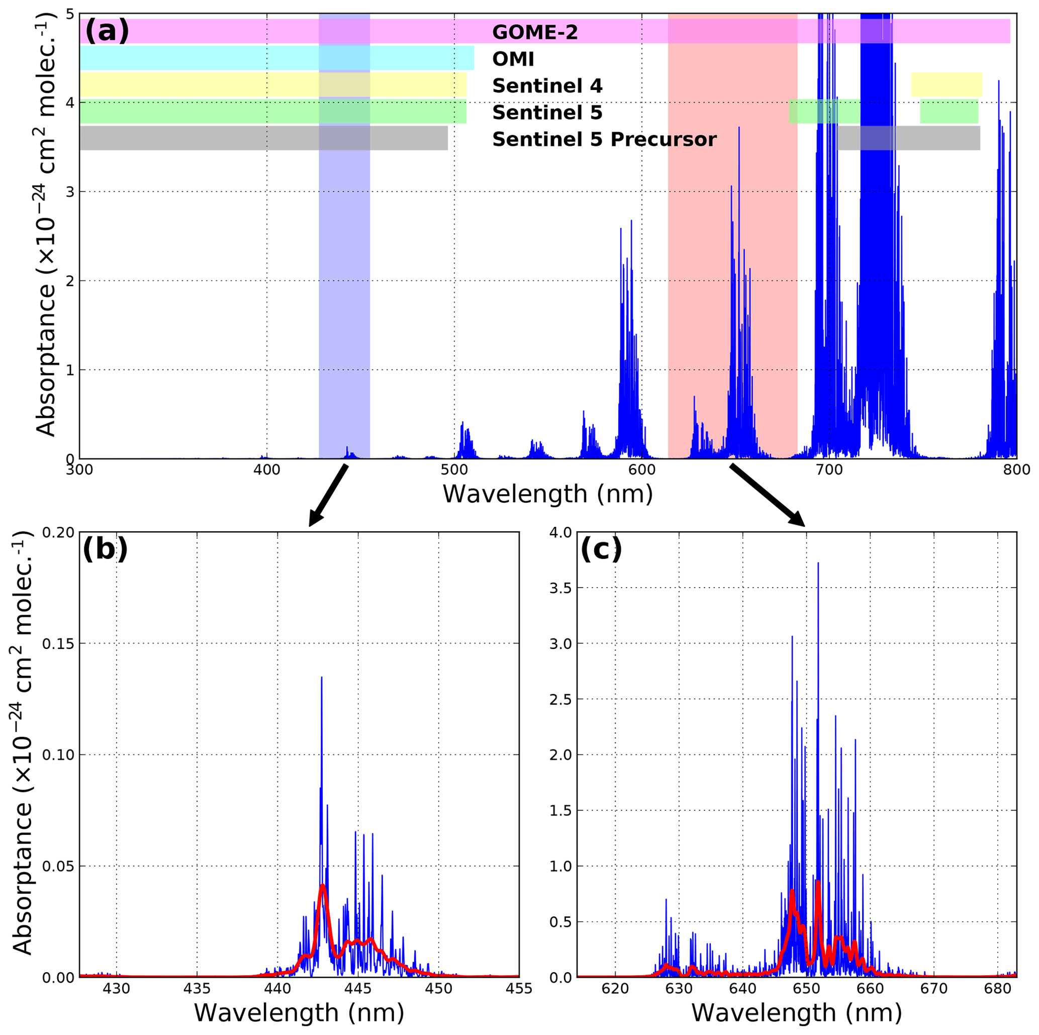
Figure 1 Water vapor absorption cross section. (a) The horizontal bars show the spectral band available to various satellite sensors. The wavelength range used in this study and the operational GOME-2 products are highlighted in blue and red, respectively. An enlargement of the blue and red bands in (a) is shown in (b) and (c), respectively. The red curves show the water vapor absorption cross section convoluted with the instrument slit function. Note that the scale of the y axis of each plot is different.

Wagner et al. (2013)Wang et al. (2014)Wang et al. (2016)

Table 1 Parameters and settings of water retrieval in the blue band used in previous studies and this work.

The objective of this study is to develop a TCWV-retrieval algorithm for spectroscopic satellite observations which fulfills the following requirements. First, the algorithm should be feasible for the current and forthcoming satellite sensors such as OMI, S5P, S4 and S5. Second, the retrieval should not rely on input from the chemistry transport model (CTM) to avoid propagating model errors into the climatological measurement records. Last, the retrieval should provide a realistic error estimation as measurement uncertainty is an important parameter for data assimilation and future harmonization of satellite data. Based on the results from previous studies, we have further optimized the spectral analysis settings for the TCWV retrieval and developed a statistical analysis approach to optimize the a priori water vapor profile used in the retrieval. In addition, a comprehensive error estimation is also included in the new water vapor retrieval algorithm. The developed algorithm has been implemented to retrieve TCWV from GOME-2 observations; in the future, we will extend the application to other, similar satellite sensors. For validation, the new TCWV data set retrieved from GOME-2 observations is compared to the GOME-2 operational product, ground-based sun photometer and radiosonde measurements.

The paper is organized as follows. Section 2 describes all instruments and data sets used in this study. The concept of the TCWV retrieval is presented in Sect. 3.1. The description of the spectral retrieval of water vapor slant columns is shown in Sect. 3.1.1. Section 3.1.2 presents the iterative optimization method for the conversion of satellite measurement of water vapor slant columns to total columns. A detailed error estimation is presented in Sect. 3.1.7. The validation of the GOME-2 TCWV is shown in Sect. 4. Section 4.1 presents the comparison against the GOME-2 operational product. The comparison against sun photometer and radiosonde data is shown in Sect. 4.2 and 4.3, respectively. Discussions of the discrepancies between different data sets are presented in Sect. 5. Finally, the conclusion is drawn in Sect. 5.3.

2 Instruments and data sets

In this section, the GOME-2 instruments and the level 1B products used in the retrieval are described. Brief descriptions of the operational GOME-2 TCWV product, sun photometer TCWV data set and the radiosonde measurements used to validate the new GOME-2 TCWV data are presented. In addition, the ERA-Interim data set used for the statistical analysis of water vapor vertical distribution is also presented.

2.1 The GOME-2 instruments

The Global Ozone Monitoring Experiment 2 (GOME-2) are passive nadir-viewing, satellite-borne spectrometers on board the European Organisation for the Exploitation of Meteorological Satellites (EUMETSAT) Metop series of satellites. The Metop satellites orbit at an altitude of ∼820 km on sun-synchronous orbits with a 29 d (412 orbits) repeat cycle and a local Equator overpass time of 09:30 LT (local time) on the descending node. Metop-A, the first Metop satellite, was launched on 19 October 2006. Metop-B was launched 6 years later on 17 September 2012. The third Metop satellite, Metop-C, was launched on 7 November 2018. All GOME-2 instruments are currently in operation. A more detailed introduction to the Metop series of satellites can be found in Klaes et al. (2007).

The GOME-2 instruments are optical spectrometers equipped with scanning mirrors which enable across-track scanning in the nadir and sideways views for polar coverage (Callies et al., 2000). Each GOME-2 instrument consists of four detectors covering a wavelength range of 240–790 nm, with a spectral resolution ranging from 0.26 to 0.51 nm. The nominal spatial resolution of the instruments is 80 km (across track) × 40 km (along track) for the forward scan, and the spatial resolution is reduced to 240 km (across track) × 40 km (along track) for the backward scan. The scanning swath width of the GOME-2 instruments is about 1920 km. After the GOME-2 instrument on board the Metop-B satellite (hereafter GOME-2B) went into a tandem operation with Metop-A in July 2013, the across-track spatial resolution of the GOME-2 instrument on board the Metop-A satellite (hereafter GOME-2A) was doubled, with the spatial coverage of a swath reduced to 960 km. The spatial resolution and coverage of GOME-2B remains unchanged. A more detailed description of the GOME-2 instruments can be found in Munro et al. (2016). In this study, we focus on the results from GOME-2A as it provides longer-term observations. GOME-2B results are shown mainly for the investigation of the consistency between the sensors.

2.2 GOME-2 level 1B data

The first step in GOME-2 data processing is the conversion of the detector signal (level 0 data) to geolocation and radiometric-calibrated radiance and irradiance data (level 1B data). GOME-2 observations taken before 25 June 2015 were processed by the level 1B processor version 6.0, while GOME-2 data taken after 25 June 2015 were processed by the updated level 1B processor version 6.1. The processor update mainly resolved spectral artefacts in the GOME-2 on-ground calibration key data. The spectral artifact in the level 1B data is due to the incomplete removal of the xenon line in the GOME-2 calibration key data. The calibration key data were taken during the preflight on-ground calibration, and the calibration key data are used as input for the level 0 to level 1B data processing. The effect of the spectral contamination in level 1B data processed by the version 6.0 processor is significant at the blue band (Band 3) and more significant for wavelengths longer than 460 nm (Azam et al., 2015). The improvement of level 1B data has been reported to have a significant impact on the NO₂ retrieval in the blue band, reducing the NO₂ columns by 6 %–23 % (Liu et al., 2019).

2.3 Operational GOME-2 TCWV product

The operational GOME-2 water vapor product is processed by the German Aerospace Center (DLR) within the framework of EUMETSAT's Satellite Application Facility on Atmospheric Composition Monitoring (AC SAF), using the GOME Data Processor (GDP) version 4.8. The product is used as reference to validate the TCWV retrieved in the blue band. The operational algorithm retrieves water vapor slant columns in the wavelength range of 614–683 nm. The conversion of slant columns to vertical columns uses air mass factors (AMFs) derived from oxygen slant columns measured in the same spectral band. Water vapor absorption in the red band is much stronger (more than an order of magnitude) than that in the blue spectral range (see Fig. 1), thus, yielding better signal-to-noise ratios. In addition, the retrieval of water vapor in the red band uses air mass factors derived from oxygen measurements at the same wavelength range, which reduces the dependency on the numerical calculation of radiative transfer in the atmosphere (Grossi et al., 2015). The operational GOME-2 water vapor product has been validated intensively by radiosonde and Global Positioning System (GPS) measurements (Antón et al., 2015; Román et al., 2015; Kalakoski et al., 2016; Vaquero-Martínez et al., 2018). The operational product has been reported to significantly underestimate the TCWV over central Africa and India; it overestimates the TCWV over oceans in the tropics during summer in the Northern Hemisphere (Grossi et al., 2015). Compared to radiosonde and GPS data, the operational GOME-2 water vapor product has, in general, a dry bias of 3 %–11 % (Antón et al., 2015; Román et al., 2015; Kalakoski et al., 2016; Vaquero-Martínez et al., 2018).

2.4 Sun photometer measurements

The CIMEL CE-318 sun photometers are used in the AERosol RObotic NETwork (AERONET) to measure direct sun and sky radiance at multiple wavelengths (Holben et al., 1998). These sun photometer observations not only provide information on aerosol optical properties (Holben et al., 2001) but also on columnar water vapor content (Alexandrov et al., 2009). Water vapor columns are retrieved from sun photometer observations in the near infrared (NIR) at 940 nm where water vapor absorption is rather strong. The inversion of water vapor columns is based on the attenuation of radiation through the atmosphere. A more detailed description of the water vapor retrieval algorithm can be found in Alexandrov et al. (2009). Water vapor columns are provided in the standard AERONET product. The AERONET water vapor product has also been validated by microwave radiometry, GPS and radiosondes measurements (Pérez-Ramírez et al., 2014). The sun photometer measurements are, in general, underestimating the columnar water vapor by 6 %– 9 % (Pérez-Ramírez et al., 2014). Cloud-screened and quality-assured level 2.0 data are used in this study. In this work, all AERONET stations providing co-located columnar water vapor measurements from 2008 to 2018 are used to validate the new GOME-2 water vapor retrieval results. In total, there are 905 AERONET stations providing co-located data with GOME-2. The locations of these AERONET stations are indicated in Fig. 2 as red triangles.

Figure 2 Locations of sun photometer (red triangles) and radiosonde (blue circles) stations providing co-located TCWV measurements with GOME-2 satellite observations. The size of the markers is proportional to the number of valid observations available.

2.5 Radiosonde measurements

Radiosonde data are taken from the Integrated Global Radiosonde Archive version 2 (IGRA2) database. The database is managed by the National Centers for Environmental Information (NCEI) of the National Oceanic and Atmospheric Administration (NOAA). The IGRA2 database includes quality-assured radiosonde measurements from over 2700 globally distributed stations. The measurements consist of temperature, relative humidity, dew point depression, wind direction and wind speed at multiple pressure levels. The IGRA2 radiosonde data are publicly available on the website of NCEI (https://www.ncdc.noaa.gov/data-access/weather-balloon/integrated-global-radiosonde-archive, last access: 30 July 2020). A more detailed description of the radiosonde data can be found in Durre et al. (2006). Compared to ground-based observations, the radiosonde measurements of TCWV show an error of ∼5 %, with bias ranging from −1.19 to 1.01 kg m⁻² (Wang and Zhang, 2008; Van Malderen et al., 2014). In this study, all radiosonde stations providing co-located columnar water vapor measurements from 2008 to 2018 are used to validate the GOME-2 water vapor measurements in the blue band. The locations of the 578 radiosonde stations providing co-located data are indicated in Fig. 2 as blue circles.

2.6 ERA-Interim reanalysis data

ERA-Interim is a global atmospheric reanalysis data set produced by the European Centre for Medium-Range Weather Forecasts (ECMWF; Dee et al., 2011; Berrisford et al., 2011). The ERA-Interim reanalysis data covers a long time period, since 1979, and provides consistent data on a global scale for the analysis of long-term variation in water vapor in the atmosphere. The reanalysis data are produced with a data assimilation scheme, which combined various measurements as prior information from model forecasts. The original data set is in a spatial resolution of ∼80 km (T255 Spectral) on 60 vertical layers extending from the surface up to 0.1 hPa. The data are then transformed to the latitude–longitude (LL) coordinate system, with a horizontal resolution of $\mathrm{0.75}{}^{\circ }\times \mathrm{0.75}{}^{\circ }$, through the ECMWF's Meteorological Archival and Retrieval System (MARS). The vertical resolution of the data set varies depending on the surface pressure; details of the data set can be found in Dee et al. (2011), Berrisford et al. (2011). TCWV is retrieved from the system with a temporal resolution of 6 h. The ERA-Interim data from 2008 to 2018 are used in the statistical analysis of water vapor vertical distribution and the relation to their total column amount.

3 Methodology

3.1 The blue band TCWV retrieval

The GOME-2 water vapor retrieval algorithm in the blue spectral range follows the classical differential optical absorption spectroscopy (DOAS) approach, which is a standard spectroscopic method for the retrieval of weakly absorbing trace gases (Platt and Stutz, 2008). The method consists of two major steps. The first step is the retrieval of water vapor slant columns. The second step is the conversion of the water vapor slant columns to vertical columns. A comprehensive error estimation is also included in the retrieval. Details of the retrieval algorithm and error estimation are presented in the following.

3.1.1 Water vapor slant column retrieval

Typical absorption spectroscopy describes the attenuation properties of radiation along an optical path with the Beer–Lambert–Bouguer law. For satellite measurements, the equation can be written as Eq. (1) as follows:

$$\begin{array}{}\text{(1)}& \begin{array}{rl}I\left(\mathit{\lambda }\right)& =I_{\mathrm{0}}\left(\mathit{\lambda }\right)\\ & \cdot \exp \left(-{\mathit{\epsilon }}_{\mathrm{M}}\left(\mathit{\lambda }\right)-{\mathit{\epsilon }}_{\mathrm{R}}\left(\mathit{\lambda }\right)-L\sum _{i=\mathrm{1}}^n{\mathit{\sigma }}_i\left(\mathit{\lambda }\right)c_i\right)\cdot R\left(\mathit{\lambda }\right),\end{array}\end{array}$$

where I₀(λ) refers to the direct sun irradiance spectrum taken at the top of atmosphere (TOA), while I(λ) is the earthshine radiance spectrum taken by looking down from space towards the nadir direction and measuring sunlight reflected by the Earth's surface and atmosphere. L represents the effective optical path length from TOA to the Earth's surface and reflected from the Earth's surface back to the satellite. σ_i denotes the absorption cross section of gas i, and c_i is its average concentration along the effective optical path. ε_M and ε_R are the Mie and Rayleigh extinction integrated along the light path, respectively. R(λ) represents the reflectance of the Earth. The optical density τ(λ) can then be calculated by taking logarithm of the ratio between I₀(λ) and I(λ) as shown in Eq. (2) as follows:

$$\begin{array}{}\text{(2)}& \mathit{\tau }\left(\mathit{\lambda }\right)=\ln \left({\displaystyle \frac{I_{\mathrm{0}}\left(\mathit{\lambda }\right)\cdot R\left(\mathit{\lambda }\right)}{I\left(\mathit{\lambda }\right)}}\right).\end{array}$$

In practice, Eq. (1) cannot be directly applied for trace gas retrieval, as some of the extinction processes, i.e., Mie and Rayleigh scattering, are not quantified. The DOAS method unitizes the fact that atmospheric scattering processes only show broadband spectral characteristics, while trace gases exhibit narrow band absorption structures (Platt and Stutz, 2008). Therefore, the optical density τ(λ) can be separated into narrow band (or differential band) τ^′(λ) and broadband τ_b(λ) contributions. The broadband contribution τ_b can be approximated by a low-order polynomial p(λ). The broadband structures in R(λ) can also be accommodated by p(λ), and narrow band features in R(λ) can be included as pseudo cross sections in the spectral fit. Thus, the equation can be rewritten as Eq. (3) as follows:

$$\begin{array}{}\text{(3)}& \mathit{\tau }\left(\mathit{\lambda }\right)=\mathit{\tau }{}^{\prime }\left(\mathit{\lambda }\right)+{\mathit{\tau }}_{\mathrm{b}}\left(\mathit{\lambda }\right)=L\cdot \sum _{i=\mathrm{1}}^n{\mathit{\sigma }}_i\left(\mathit{\lambda }\right)c_i+p\left(\mathit{\lambda }\right).\end{array}$$

Characteristic absorption features of different trace gases are then used to determine their concentrations c_i along the effective optical path L.

Rothman et al. (2010)Lampel et al. (2015)Vandaele et al. (2002)Brion et al. (1998)Thalman and Volkamer (2013)Pope and Fry (1997)

Table 2 The spectral fit settings for the retrieval of water vapor slant column.

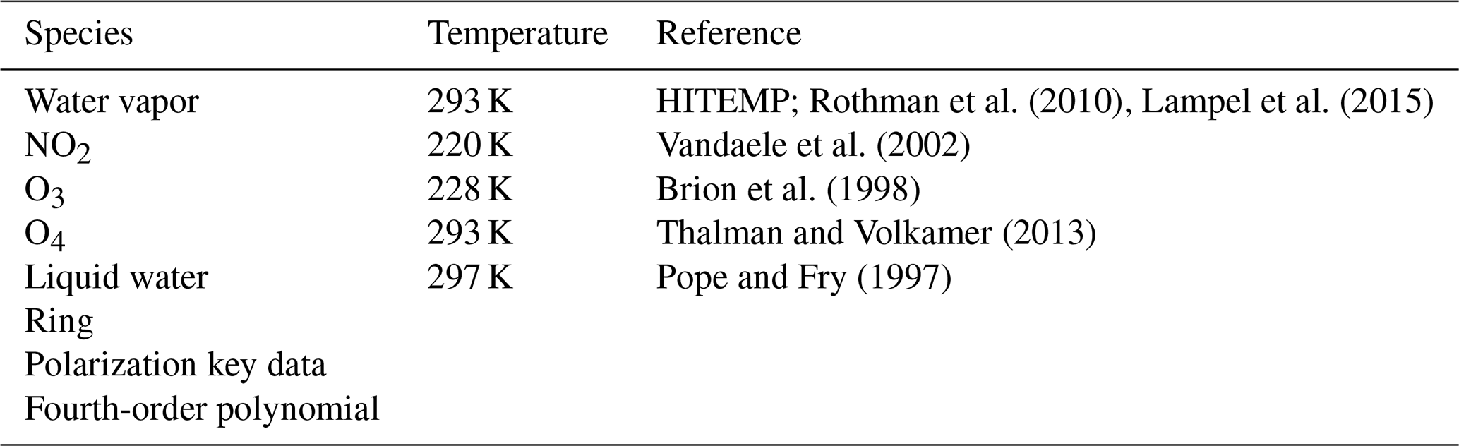
Slant column densities (SCDs) of water vapor are retrieved from GOME-2 spectra by applying the DOAS spectral fitting technique. The SCD is defined as the integrated concentration along the optical path from TOA through the atmosphere to the Earth's surface and reflected back to the satellite sensor (L×c_i). The DOAS spectral fit is applied to the wavelength range of 427.7–455 nm. The following absorption cross sections are employed in the DOAS fit, namely water vapor at 293 K from the HITEMP database (Rothman et al., 2010) and scaled by Lampel et al. (2015); NO₂ at 220 K (Vandaele et al., 2002); O₃ at 228 K (Brion et al., 1998); O₄ at 293 K (Thalman and Volkamer, 2013); liquid water at 297 K (Pope and Fry, 1997); and a Ring spectrum. Two additional GOME-2 polarization key data are also included in the DOAS fit to correct for remaining level 1B calibration issues caused by polarization. Details of the spectral fit settings are shown in Table 2. These cross sections are first convoluted with the effective instrument slit function to the instrument spectral resolution. The effective slit function is derived by convolving a high-resolution reference solar spectrum (Chance and Kurucz, 2010), with a stretched preflight GOME-2 slit function, and aligning to the GOME-2 daily irradiance measurements, with stretch factors as fit parameters. Similar approaches with different spectral retrieval settings have also been used to retrieve slant column water vapor from different satellite sensors, e.g., GOME-2 and OMI (Wagner et al., 2013; Wang et al., 2014, 2016). A brief summary of the previous studies is presented in Table 1. An example of the spectral fitting retrieval of a GOME-2A spectrum taken on 1 July 2008 over the Pacific Ocean is shown in Fig. 3.

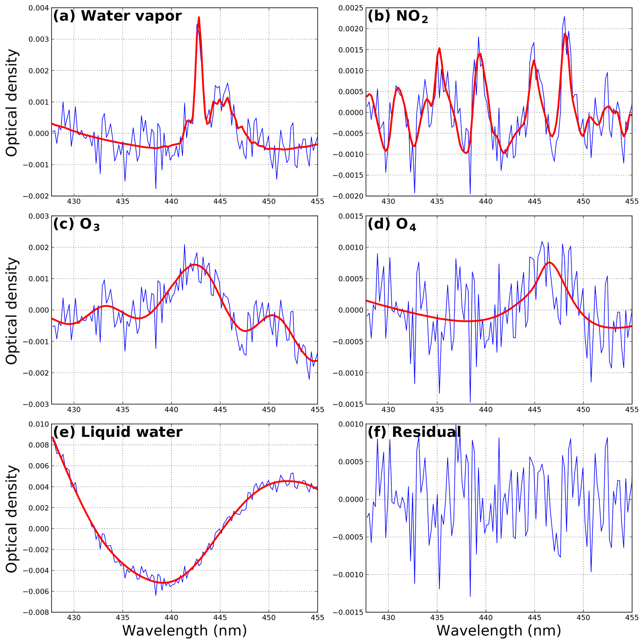
Figure 3 An example of the DOAS retrieval of water vapor slant columns from a GOME-2A spectrum over the Pacific Ocean. The retrieved water vapor slant column is 30.6 kg m⁻². The blue curves show measured optical density, with the broadband attenuation removed by subtracting a fourth-order polynomial, and the red curves show the optical density of the scaled reference absorption cross sections.

The spectral-fitting window is optimized for water vapor retrieval, which includes a relatively strong water vapor absorption structure at about 442 nm. Including liquid water absorption in the analysis effectively eliminates the interference of liquid water and reduces the systematic error above surfaces covered by water (Wang et al., 2014, 2016). The spectral-fitting window is optimized to minimize the influence from spectral contamination in the GOME-2 level 1B data. This issue has been reported to be more significant for wavelengths longer than 460 nm (Azam et al., 2015); therefore, the fitting window has been limited to 455 nm. Recent studies reported that using the water vapor cross section from the HITRAN 2008 database (Rothman et al., 2009) results in a better agreement with reference measurements (Wang et al., 2019; Borger et al., 2020). Therefore, we did a sensitivity analysis with both cross sections. The result shows that water vapor slant columns retrieved with the HITRAN 2008 cross section are 1 %–2 % higher. The increase is also more significant over high altitudes and would further enhance the positive bias over these areas. In addition, the root mean square of the spectral fit residual using the HITEMP 2010 cross section is slightly (∼3 %) smaller. Therefore, this cross section is used in the retrieval. A fourth-order polynomial is included in the DOAS fit to remove the broadband spectral structures of Rayleigh scattering and lower-order Mie scattering, broadband trace gas absorption, and instrumental effects. Using a polynomial with a higher order is likely to improve the DOAS fit and minimize the fit residual, but it is difficult to justify the physical meaning. Shift and stretch parameters of radiance spectra are also fitted in the spectral-fitting process to compensate for the instability due to small thermal variations of the spectrograph. The spectral fitting results are the slant columns of water vapor. Figure 4a shows the water vapor slant columns retrieved from GOME-2A observations on 1 July 2008 (orbit 8813–8826). The corresponding slant column uncertainties and the root mean square of the spectral fit residual are shown in Fig. 4b and c, respectively. As expected, the retrieved water vapor slant columns show higher values over tropical regions and lower slant columns at upper latitudes. In addition, the slant column uncertainties and the root mean square of the spectral fit residual are significantly higher at both ends of the satellite orbits. There, the observations are taken with a very high solar zenith angle and, thus, lower radiance intensity and signal-to-noise ratio. The mean spectral fitting uncertainty is about 5.2 kg m⁻² over the tropics (30^∘ S–30^∘ N), which is equivalent to a mean relative error of ∼13.9 %. The average root mean square of the spectral fitting is $\mathrm{9.2}\times {\mathrm{10}}^{-\mathrm{4}}$.

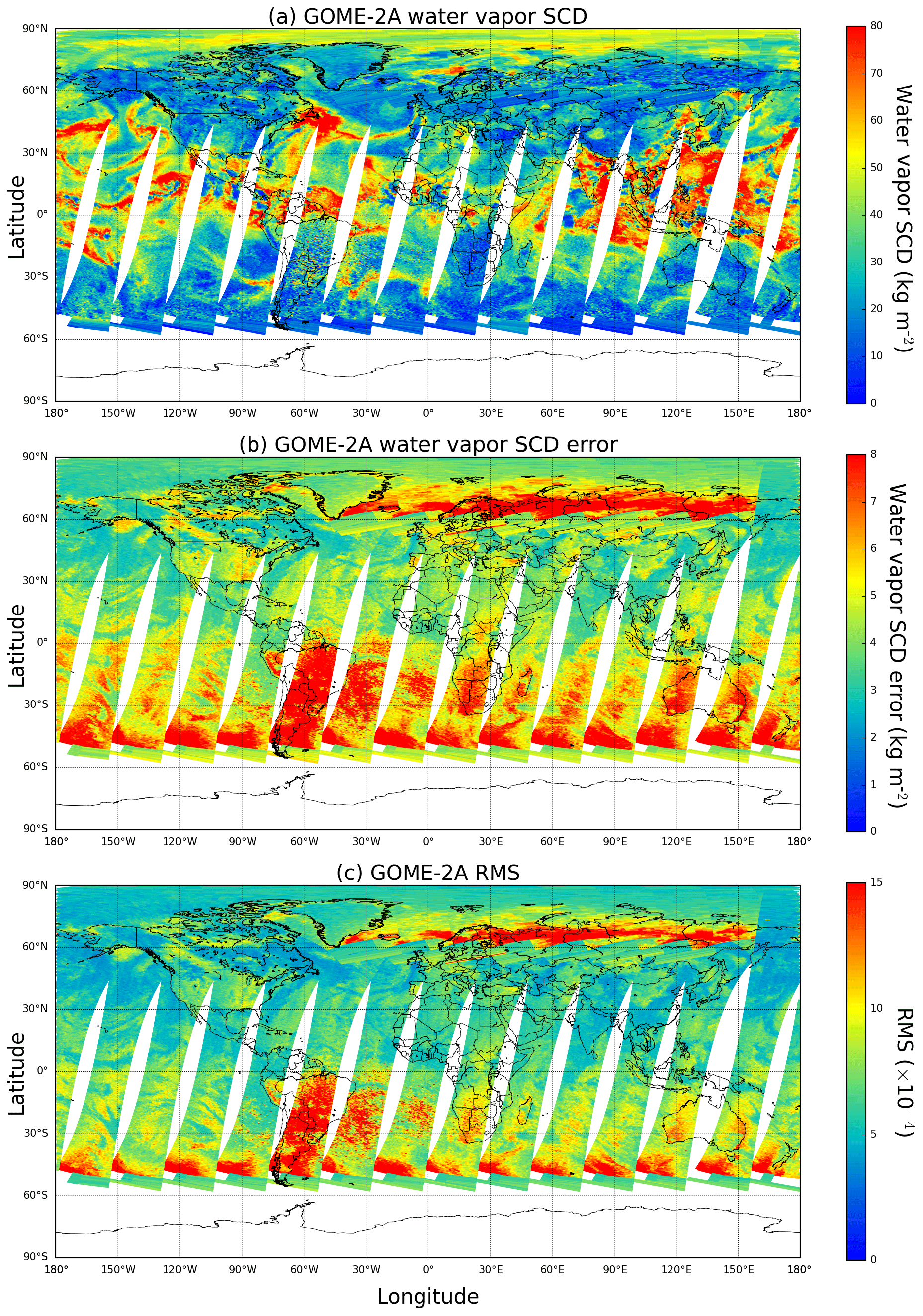
Figure 4 (a) Slant column densities of water vapor retrieved from GOME-2 observations on 1 July 2008 (orbit 8813–8826). (b) The corresponding water vapor slant column uncertainties and (c) the root mean square of the spectral fit residual.

3.1.2 Air mass factor

The next step in the TCWV retrieval is the conversion of water vapor SCDs to vertical column densities (VCDs). The VCD (or total column) is defined as the vertical integral of water vapor from the surface to the top of atmosphere. The SCD to VCD conversion is accomplished by using the concept of the air mass factor (AMF; Solomon et al., 1987). As water vapor SCDs are retrieved within a relatively narrow spectral window, we can assume the wavelength dependency of the optical path is negligible. Thus, the AMFs need only be calculated at a representative wavelength. Due to the relatively strong water vapor absorption feature at 442 nm, the AMFs are calculated at this wavelength. The AMF can be expressed as Eq. (4) as follows:

$$\begin{array}{}\text{(4)}& \text{AMF}={\displaystyle \frac{\text{SCD}}{\text{VCD}}}.\end{array}$$

Light traveling in the atmosphere can be scattered by air molecules, aerosols and clouds, resulting in a complex optical path. To resolve the optical path and the box air mass factor (ΔAMF), comprehensive multiple scattering radiative transfer calculations are required. The ΔAMF is defined as the AMF of each individual vertical layer. Typically, the height-dependent air mass factor can be decoupled from the vertical distribution of optically thin absorbers (Palmer et al., 2001). As a result, the AMF can then be calculated from the ΔAMF using Eq. (5) as follows:

$$\begin{array}{}\text{(5)}& \text{AMF}={\displaystyle \frac{\text{SCD}}{\text{VCD}}}={\displaystyle \frac{\sum _{l=\mathrm{surface}}^{l=\mathrm{TOA}}\mathrm{\Delta }{\text{AMF}}_l\times \mathrm{\Delta }{z}_l\times c_l}{\sum _{l=\mathrm{surface}}^{l=\mathrm{TOA}}\mathrm{\Delta }{z}_l\times c_l}},\end{array}$$

where Δz_l and c_l are the thickness and the number density of the absorber at layer l, respectively. c_l is taken from the a priori profile. The ΔAMFs are independent of the vertical distribution of the absorber but strongly dependent on viewing geometry, solar position, surface albedo and surface altitude.

3.1.3 Box air mass factor look-up table

The ΔAMFs can be calculated using a radiative transfer model. To reduce the processing time, ΔAMFs are precalculated with a number of representative observation and solar geometries, surface albedo, and surface pressure and are stored in a look-up table. In the current version of the retrieval algorithm, the ΔAMF look-up table is calculated with the radiative transfer model VLIDORT version 2.7 (Spurr, 2008) at 442 nm, with an aerosol-free US standard atmosphere (Anderson et al., 1986). The ΔAMFs for each particular GOME-2 observation can then be derived by interpolating within the look-up table. Details of the parameterization of the ΔAMF look-up table are shown in Table 3.

Table 3 Parameters in the box air mass factor look-up table.

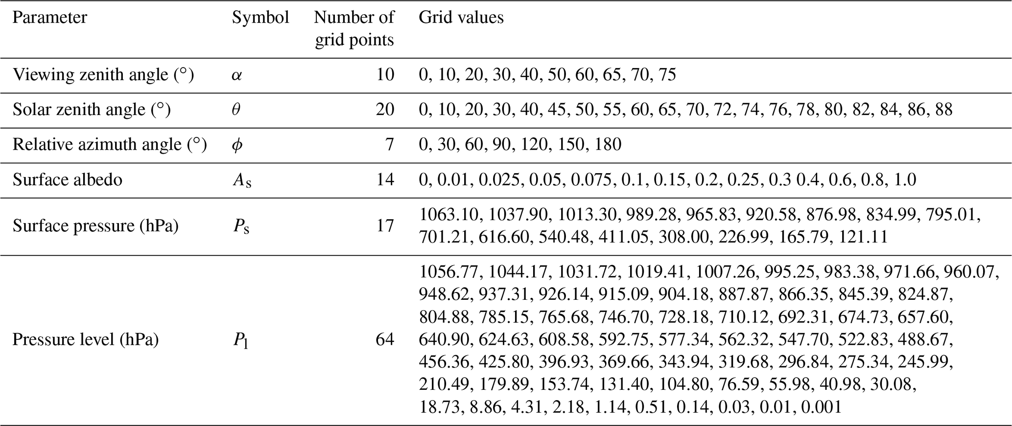
For retrieval, the ΔAMF look-up table is interpolated linearly in the surface albedo (A_s), relative azimuth angle (ϕ), cosine of the solar zenith angle (cos θ) and cosine of the viewing zenith angle (cos α) dimensions, while a nearest-neighbor interpolation is applied to the surface pressure dimension. In the current version of the retrieval algorithm, surface albedo is taken from the climatology monthly minimum Lambertian-equivalent reflector (LER) product version 2.1 at 440 nm, derived from observations of the corresponding GOME-2 sensor (Tilstra et al., 2017) and spatially interpolated to the GOME-2 measurement locations. The GOME-2 surface LER (version 2.1) data set has the advantage of using more recent observations (2007–2013) and accounting for the degradation of GOME-2 level 1 data. The GOME-2 surface LER (version 2.1) data set is in a resolution of $\mathrm{0.5}{}^{\circ }\times \mathrm{0.5}{}^{\circ }$, with an increased resolution of $\mathrm{0.25}{}^{\circ }\times \mathrm{0.25}{}^{\circ }$ along coastlines. The viewing and solar geometries are taken from the GOME-2 level 1B product. The resulting ΔAMF profile is then linearly interpolated to match the vertical grid of the water vapor a priori profile. The AMF can then be calculated following Eq. (5).

3.1.4 A priori water vapor vertical profile

The vertical distribution of water vapor is important for the conversion of slant columns of water vapor to vertical columns as expressed in Eq. (5). Most of the trace gas retrievals from satellite measurements in the UV and Vis spectral range use vertical profile information from chemistry transport model simulations (e.g., Wang et al., 2014, 2016; Krotkov et al., 2017; De Smedt et al., 2018). Previous studies use a priori profiles from GEOS-5 and MERRA-2 model products to retrieve TCWV from OMI observations (Wang et al., 2014, 2016). In this study, we used the statistical analysis of historical profiles' a priori information so that the influences from model simulation were greatly reduced and more suitable for climatological study. We developed an iterative approach to optimize the a priori water vapor vertical profile used in the satellite retrieval to make the satellite measurements independent from model simulations and to avoid propagating model errors into the measurement. The iterative a priori profile optimization approach is based on the statistical analysis of water vapor vertical distribution over 11 years from 2008 to 2018. Figure 5 shows the statistical analysis of water vapor profiles from the ECMWF ERA-Interim reanalysis data (Dee et al., 2011; Berrisford et al., 2011) over a small region of the Pacific Ocean (5^∘ S–5^∘ N, 180–170^∘ W) in July 2008–2018. Water vapor profiles are sorted by their total column densities into eight ranges from 20 up to 60 kg m⁻². Color-coded lines indicate the mean profile of each range, while the shading represents the 1σ standard deviation variation of the water vapor mixing ratio. The normalized mean profiles for each range are also indicated in Fig. 5i. These profiles are normalized by dividing their total columns and multiplying them with the mean total column calculated from all measurements. The analysis result shows that water vapor vertical profile shapes are strongly related to their own column densities. Water vapor profiles with similar total columns show a very similar vertical distribution. Water vapor is typically concentrated close to the surface below 800 hPa when the total column is small (i.e., less than 30 kg m⁻²). It starts to extend to higher altitudes, with increasing total column, and this changes the profile shape. A much larger portion of water vapor is located above 800 hPa when the total column is larger than 40 kg m⁻². The small standard deviation of the water vapor mixing ratio profile also indicates that the water vapor profile shape only varies slightly within each range.

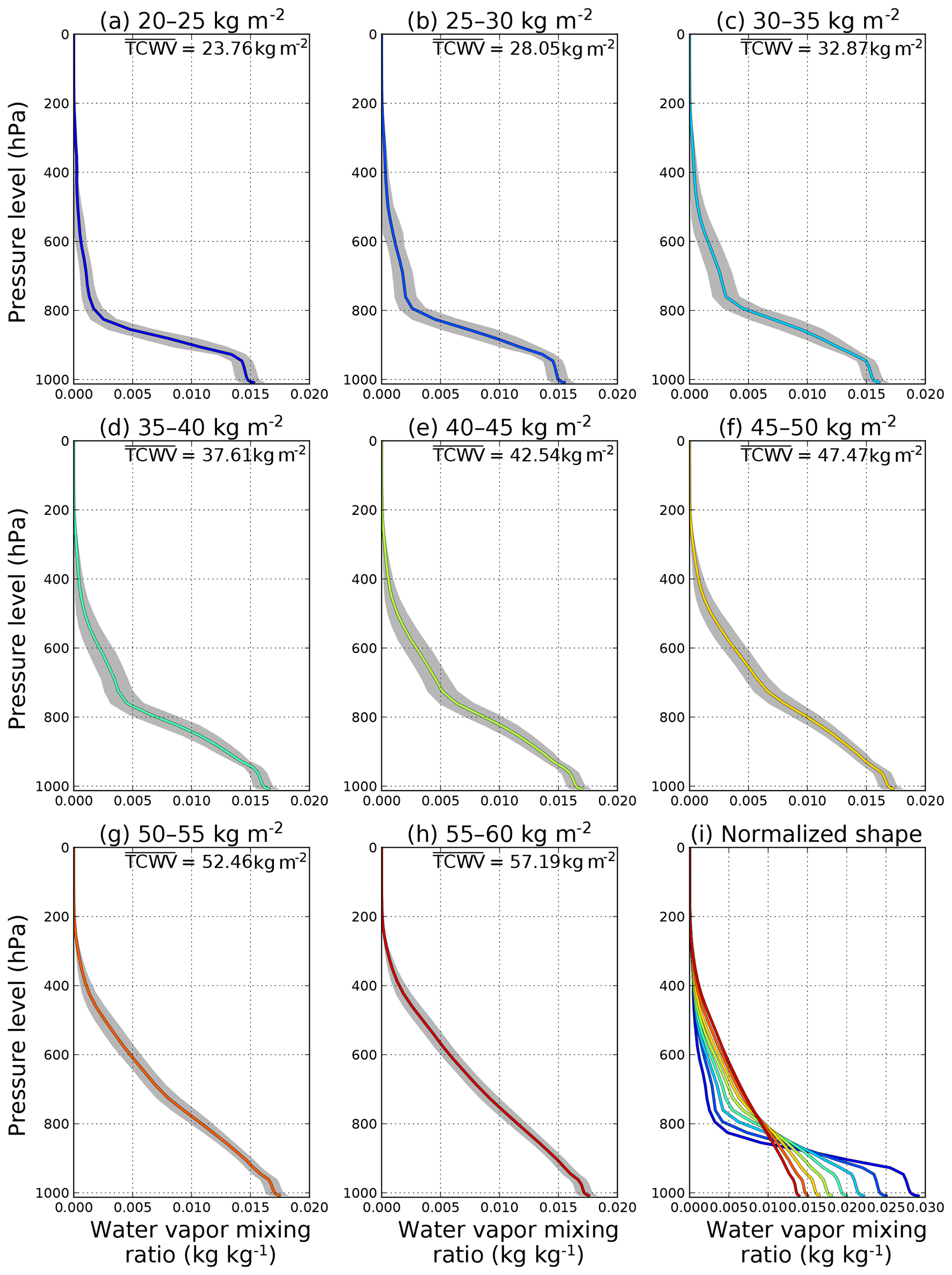
Figure 5 Statistical analysis of water vapor vertical profiles from ECMWF ERA-Interim reanalysis data over a small region of the Pacific Ocean (5^∘ S–5^∘ N, 180–170^∘ W) in July 2008 to 2018. Water vapor profiles are sorted by their total column density into eight ranges, which are (a) 20–25 kg m⁻², (b) 25–30 kg m⁻², (c) 30–35 kg m⁻², (d) 35–40 kg m⁻², (e) 40–45 kg m⁻², (f) 45–50 kg m⁻², (g) 50–55 kg m⁻² and (h) 55–60 kg m⁻². The shading indicates the 1σ standard deviation variation of water vapor mixing ratio. Panel (i) shows the normalized mean water vapor profile shapes of these eight ranges.

By making use of the characteristic that water vapor profile shapes are strongly correlated to their total columns, we have formulated a water vapor vertical profile shape look-up table for the entire globe with a spatial resolution of 0.75^∘. Water vapor profiles are sorted into five ranges for each geolocation and for each month of the year. The mean profiles, total columns and standard deviation of total columns for each range are stored in a look-up table. The water vapor vertical profile shape look-up table is interpolated linearly in the spatial dimension to the satellite measurement location for each range. The iterative optimization of the a priori water profile begins by using the overall mean profile of the satellite measurement location of the corresponding month. This mean water vapor profile is then used together with the corresponding ΔAMFs to calculate an initial AMF following Eq. (5). The water vapor slant column is divided by this initial AMF to retrieve the initial vertical column. The look-up table is then linearly interpolated in the total column dimension with the retrieved initial column to retrieve the corresponding vertical profile shape. The interpolated profile is again used to retrieve the second vertical column. This process repeats until the difference between the input and output water vapor column is less than 1 % or the number of iteration reaches the limit. As the retrieval of more than 99 % of GOME-2 measurements stopped within three iterations, the limit of the maximum number of iteration in the current version of retrieval is set to five.

3.1.5 Partially cloudy scene observations

Clouds are treated as opaque Lambertian surfaces in the retrieval algorithm. The treatment of partially cloudy pixels is based on the independent pixel approximation (Martin et al., 2002; Boersma et al., 2004) in which the pixel is separated into two independent parts, namely one with full cloud cover and the other one which is completely cloud free. Air mass factors are calculated separately for both clear sky and cloudy parts. Cloud information, including cloud fraction (CF), cloud albedo (A_c) and cloud top pressure (P_c), is taken from the GOME-2 operational cloud product (Loyola et al., 2007, 2010; Lutz et al., 2016). The assumption of a Lambertian cloud is more representative for optically thick clouds. Therefore, we transformed optically thin clouds to Lambertian equivalent clouds in the retrieval. As cloud albedo is directly related to the cloud optical thickness, cloud fractions are converted to an effective cloud fraction (CF_eff) using the cloud albedo and Eq. (6) as follows:

$$\begin{array}{}\text{(6)}& {\text{CF}}_{\mathrm{eff}}={\displaystyle \frac{\text{CF}\times A_{\mathrm{c}}}{\mathrm{0.8}}}.\end{array}$$

The cloudy AMF (AMF_cld) is calculated from the ΔAMF look-up table by setting the surface pressure to cloud top pressure and replacing the surface albedo with the cloud albedo. It should be noted that the same a priori water vapor profile is assumed in both the cloudy AMF and clear-sky AMF (AMF_clr) calculations. Following Eq. (5), the calculation of SCD for the cloudy scene is insensitive to water vapor below cloud, and ΔAMFs below cloud are 0. On the other hand, VCD is calculated by integrating the water vapor profile from the surface to the top of atmosphere, which includes the part below cloud. This “invisible” column below the cloud (also known as the “ghost column”) is taken from the a priori profile.

AMFs of partially cloudy pixels are calculated as the intensity-weighted average of the AMF_cld and AMF_clr. This weighting is commonly known as the intensity-weighted cloud fraction (CF_iw), which is defined by Eq. (7) as follows:

$$\begin{array}{}\text{(7)}& {\text{CF}}_{\mathrm{iw}}={\displaystyle \frac{{\text{CF}}_{\mathrm{eff}}\times I_{\mathrm{cld}}}{{\text{CF}}_{\mathrm{eff}}\times I_{\mathrm{cld}}+\left(\mathrm{1}-{\text{CF}}_{\mathrm{eff}}\right)\times I_{\mathrm{clr}}}},\end{array}$$

where I_cld and I_clr represent the radiance intensity for the cloudy and clear-sky scenes, respectively. The radiance intensities are precalculated using the radiative transfer model VLIDORT at 442 nm for a number of representative observation and solar geometries, surface albedo and surface pressure and are stored in a look-up table. The settings of the intensity look-up table are the same as the ΔAMF look-up table but without the pressure level dimension. The AMF can then be calculated with Eq. (8) as follows:

$$\begin{array}{}\text{(8)}& \text{AMF}={\text{AMF}}_{\mathrm{cld}}\times {\text{CF}}_{\mathrm{iw}}+{\text{AMF}}_{\mathrm{clr}}\times \left(\mathrm{1}-{\text{CF}}_{\mathrm{iw}}\right).\end{array}$$

The resulting AMFs are used to divide the measured slant columns and convert the water vapor slant columns into vertical columns. This AMF is used for the iterative optimization of a priori profile of partially cloudy pixels.

3.1.6 Aerosol

The presence of aerosols affects the radiative transfer in the atmosphere and may influence the retrieval of surface properties, cloud and atmospheric water vapor (Bhatia et al., 2015, 2018). As the aerosol properties, e.g., extinction profile, single scattering albedo, asymmetry parameter, etc., are unknown, there is no general and easy solution to explicitly account for aerosols in the retrieval. On the other hand, it is very difficult to separate cloud and aerosol in the cloud retrieval due to their similar optical properties. As a result, the aerosol effect is already implicitly considered in the cloud product (Boersma et al., 2004, 2011). Therefore, no additional treatment of aerosol is applied in the water vapor retrieval algorithm.

3.1.7 Error estimation

The error of the TCWV is composed of many sources. Major sources of error can be divided into two parts where one is related to the measurement itself, and the other is related to the uncertainties of assumptions in the retrieval. The uncertainty of the TCWV can be derived analytically through error propagation. As the retrieval of TCWV is separated into two major steps, namely slant column retrieval and AMF calculation, the error estimation also follows these two steps. The uncertainty of TCWV can be express as Eq. (9) as follows:

$$\begin{array}{}\text{(9)}& {\mathit{\sigma }}_{\mathrm{vcd}}^{\mathrm{2}}={\text{VCD}}^{\mathrm{2}}\times \left({\left({\displaystyle \frac{{\mathit{\sigma }}_{\mathrm{scd}}}{\text{SCD}}}\right)}^{\mathrm{2}}+{\left({\displaystyle \frac{{\mathit{\sigma }}_{\mathrm{amf}}}{\text{AMF}}}\right)}^{\mathrm{2}}\right),\end{array}$$

where σ_vcd, σ_scd and σ_amf are the uncertainty of TCWV, the error of water vapor slant column and air mass factor uncertainty, respectively. Details of the estimation of the water vapor slant column uncertainty and air mass factor error are presented in the following.

3.1.8 Slant column error

The uncertainties of water vapor slant column are mainly attributed to the instrument noise, instrument characteristics and the uncertainties related to the DOAS retrieval of the slant column. Instrument noise is expected to cause random errors, and this error can be quantified by analyzing the DOAS fit residual (Stutz and Platt, 1996). Other sources of error, related to the instrument, are the uncertainties of instrument slit function, incomplete removal of stray light and wavelength calibration uncertainties. In addition, we have uncertainties of absorption cross sections and temperature dependency of the absorption cross sections. The contributions of systematic errors to the slant column uncertainties are estimated through sensitivity tests with absorption cross section, with different effective temperature and different assumptions of instrument slit function shape. We estimated that the systematic error of the slant column is about 3 %. The total error of the slant column can be calculated with Eq. (11) as follows:

$$\begin{array}{}\text{(10)}& {\mathit{\sigma }}_{\mathrm{scd}}^{\mathrm{2}}={\mathit{\sigma }}_{{\mathrm{scd}}_{\mathrm{r}}}^{\mathrm{2}}+{\left(\mathrm{0.03}\times \text{SCD}\right)}^{\mathrm{2}},\end{array}$$

where ${\mathit{\sigma }}_{{\mathrm{scd}}_{\mathrm{r}}}$ is the random error estimated by analyzing the DOAS fit residual.

3.1.9 Clear-sky air mass factor error

The uncertainty of the AMF is mainly related to the uncertainties of each input parameter used in the AMF calculation. These input parameters include the solar and viewing geometries, surface albedo, surface pressure and water vapor vertical profile. The solar and viewing geometries are well calibrated, and their errors are mainly related to the interpolation of the box AMF look-up table. These uncertainties are negligible compared to other sources of error. The contribution to the AMF uncertainty from the remaining sources of error can be estimated by the AMF sensitivity (or Jacobian) with respect to each parameter (Boersma et al., 2004). The Jacobian is derived from the box air mass factor look-up table using the finite difference method.

In this study, surface albedo is taken from the surface reflectance climatology at 440 nm, which is derived from GOME-2 measurements from 2007 to 2013. The uncertainty of surface albedo (A_s) is assumed to be the difference between albedo derived at 425 and 440 nm to account for the small variation of albedo within the spectral fitting window. Information of the surface pressure (P_s) is taken from a digital elevation model (DEM), which is considered rather accurate, and the uncertainty of surface pressure is mostly related to the variation within the GOME-2 footprint. We have analyzed this variation of surface pressure and find it is mostly (95 %) below 10 hPa. Therefore, we set the uncertainty of P_s to 10 hPa.

The error related to the a priori vertical distribution of water vapor is determined by using the a priori water vapor from the last iteration plus 1σ standard deviation, which is also included in the look-up table. This new profile is then used to calculate the corresponding AMF. The difference between this AMF and the original AMF is taken as the uncertainty from the a priori profile. The uncertainty of the water vapor slant column can potentially affect the dynamic search of the a priori profile. As the slant column uncertainty can be much higher than the slant column itself over dry areas in the upper latitudes, considering this effect in the vertical profile uncertainty estimation would further amplify the uncertainty and results in an unrealistic high error. Therefore, we assume that this effect is well covered by the vertical profile variation and accounted for in the vertical profile uncertainty estimation. The error of the clear-sky AMF can be calculated with Eq. (11) as follows:

$$\begin{array}{}\text{(11)}& \begin{array}{rl}{\mathit{\sigma }}_{{\mathrm{amf}}_{\mathrm{clr}}}^{\mathrm{2}}& ={\left({\displaystyle \frac{\partial {\text{AMF}}_{\mathrm{clr}}}{\partial A_{\mathrm{s}}}}{\mathit{\sigma }}_{A_{\mathrm{s}}}\right)}^{\mathrm{2}}+{\left({\displaystyle \frac{\partial {\text{AMF}}_{\mathrm{clr}}}{\partial P_{\mathrm{s}}}}{\mathit{\sigma }}_{P_{\mathrm{s}}}\right)}^{\mathrm{2}}\\ & +{\left({\displaystyle \frac{\partial {\text{AMF}}_{\mathrm{clr}}}{\partial c_{\mathrm{l}}}}{\mathit{\sigma }}_{c_{\mathrm{l}}}\right)}^{\mathrm{2}},\end{array}\end{array}$$

where ${\mathit{\sigma }}_{{\mathrm{amf}}_{\mathrm{clr}}}$, ${\mathit{\sigma }}_{A_{\mathrm{s}}}$, ${\mathit{\sigma }}_{P_{\mathrm{s}}}$ and ${\mathit{\sigma }}_{c_{\mathrm{s}}}$ are the uncertainty of the clear-sky AMF, surface albedo, surface pressure and water vapor profile, respectively. This error is, in general, <5 % for GOME-2 measurements over the tropics (30^∘ S–30^∘ N).

3.1.10 Cloudy air mass factor error

The calculation of the uncertainty of the cloudy AMF is similar to the one used for the clear-sky AMF, with surface albedo and surface pressure uncertainties replaced by cloud albedo and cloud top pressure errors. In this study, the cloud top pressure error is assumed to be 50 hPa (Theys et al., 2017; De Smedt et al., 2018). Previous studies show that the error of the cloud albedo is compensated by the corresponding error of the cloud fraction, resulting a negligible net effect on trace gas retrieval (Van Roozendael et al., 2006; Lutz et al., 2016). Therefore, we assumed a cloud albedo uncertainty of 0.02 and intensity-weighted cloud fraction uncertainty of 0.02. The combined effect of the assumed cloud albedo and cloud fraction uncertainties on water vapor retrieval is comparable to the assumption with a just cloud fraction error of 0.05 (Theys et al., 2017; De Smedt et al., 2018). The error of the cloudy AMF can be expressed as Eq. (12) in the following way:

$$\begin{array}{}\text{(12)}& \begin{array}{rl}{\mathit{\sigma }}_{{\mathrm{amf}}_{\mathrm{cld}}}^{\mathrm{2}}& ={\left({\displaystyle \frac{\partial {\text{AMF}}_{\mathrm{cld}}}{\partial A_{\mathrm{c}}}}{\mathit{\sigma }}_{A_{\mathrm{c}}}\right)}^{\mathrm{2}}+{\left({\displaystyle \frac{\partial {\text{AMF}}_{\mathrm{cld}}}{\partial P_{\mathrm{c}}}}{\mathit{\sigma }}_{P_{\mathrm{c}}}\right)}^{\mathrm{2}}\\ & +{\left({\displaystyle \frac{\partial {\text{AMF}}_{\mathrm{cld}}}{\partial c_{\mathrm{l}}}}{\mathit{\sigma }}_{c_{\mathrm{l}}}\right)}^{\mathrm{2}},\end{array}\end{array}$$

where ${\mathit{\sigma }}_{{\mathrm{amf}}_{\mathrm{cld}}}$, ${\mathit{\sigma }}_{A_{\mathrm{c}}}$, ${\mathit{\sigma }}_{P_{\mathrm{c}}}$ and ${\mathit{\sigma }}_{c_{\mathrm{l}}}$ are the uncertainty of the cloudy AMF, cloud albedo, cloud top pressure and water vapor profile, respectively. The error of the cloudy AMF (${\mathit{\sigma }}_{{\mathrm{amf}}_{\mathrm{cld}}}$), in general, varies from 25 % (25th percentile) to 40 % (75th percentile) for GOME-2 measurements over the tropics (30^∘ S–30^∘ N).

3.1.11 Air mass factor error

Following Eq. (8), the uncertainty of the total AMF can be derived from the clear-sky and cloudy AMFs through error propagation. The error of the total AMF can be calculated with Eq. (13) as follows:

$$\begin{array}{}\text{(13)}& \begin{array}{rl}{\mathit{\sigma }}_{\mathrm{amf}}^{\mathrm{2}}=& ({\text{AMF}}_{\mathrm{cld}}\times {\text{CF}}_{\mathrm{iw}}{)}^{\mathrm{2}}\\ & \times \left({\left({\displaystyle \frac{{\mathit{\sigma }}_{{\mathrm{amf}}_{\mathrm{cld}}}}{{\text{AMF}}_{\mathrm{cld}}}}\right)}^{\mathrm{2}}+{\left({\displaystyle \frac{{\mathit{\sigma }}_{{\mathrm{cf}}_{\mathrm{iw}}}}{{\text{CF}}_{\mathrm{iw}}}}\right)}^{\mathrm{2}}\right)\\ & +({\text{AMF}}_{\mathrm{clr}}\times \left(\mathrm{1}-{\text{CF}}_{\mathrm{iw}}\right){)}^{\mathrm{2}}\\ & \times \left({\left({\displaystyle \frac{{\mathit{\sigma }}_{{\mathrm{amf}}_{\mathrm{clr}}}}{{\text{AMF}}_{\mathrm{clr}}}}\right)}^{\mathrm{2}}+{\left({\displaystyle \frac{{\mathit{\sigma }}_{{\mathrm{cf}}_{\mathrm{iw}}}}{\mathrm{1}-{\text{CF}}_{\mathrm{iw}}}}\right)}^{\mathrm{2}}\right),\end{array}\end{array}$$

where ${\mathit{\sigma }}_{{\mathrm{cf}}_{\mathrm{iw}}}$ is the uncertainty of the intensity-weighted cloud fraction, which is assumed to be 0.02 in the retrieval. The uncertainty of AMF (σ_amf) for GOME-2 measurements over the tropics (30^∘ S–30^∘ N) varies in a range of 6 %–22 % (25th and 75th percentile), while the error reduces to ∼6 % if the measurements are filtered for intensity-weighted cloud fraction below 0.5. The uncertainty of AMF only shows a small latitudinal dependency on surface properties (albedo) and cloud patterns, observations and solar geometries. When all measurements are considered, the uncertainty of AMF varies from 8 % (25th percentile) to 24 % (75th percentile), with a median value of 16 % while the mean error remains at ∼6 % for measurements with intensity-weighted cloud fractions below 0.5.

3.1.12 Total error

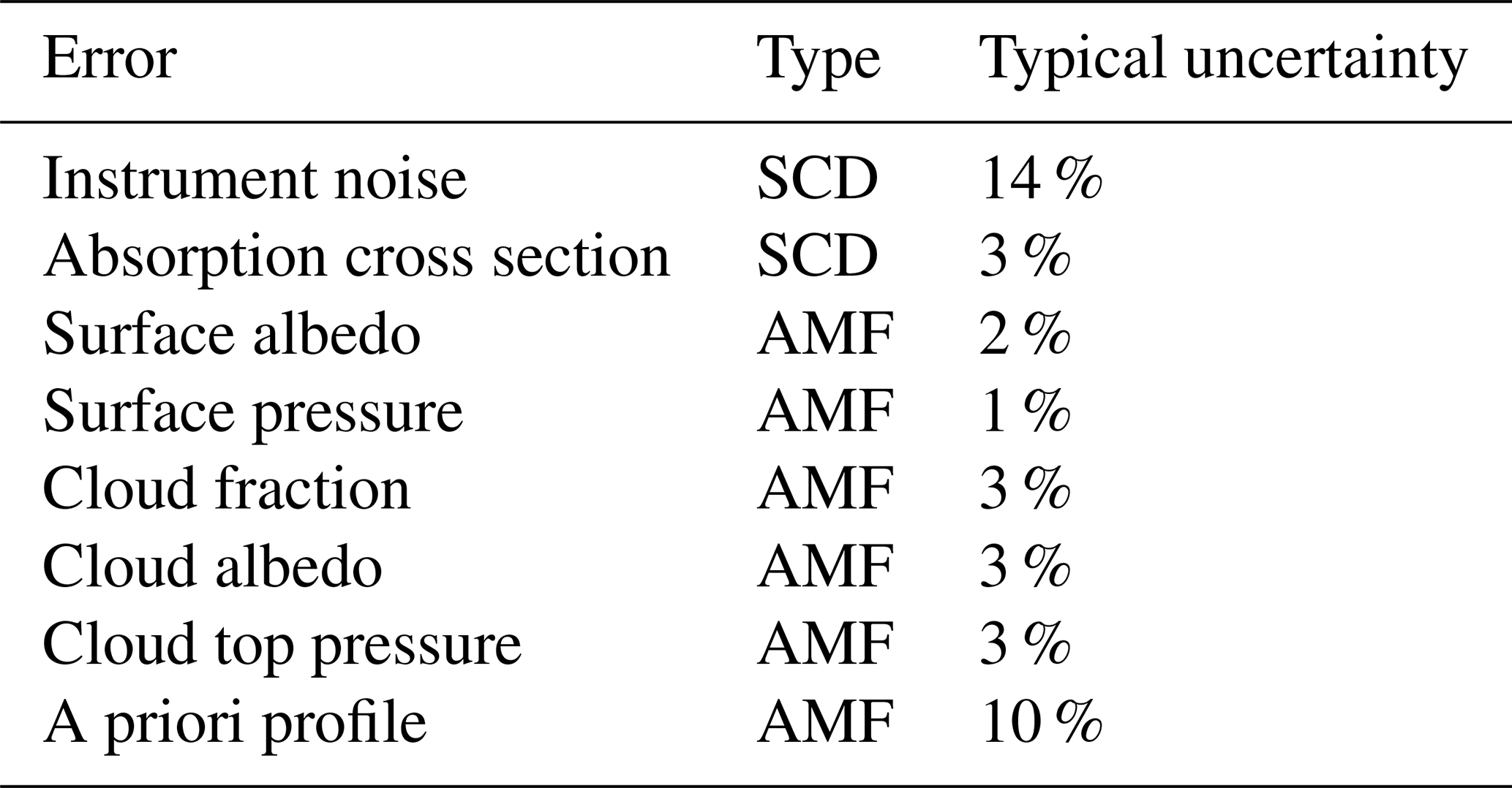
Combining the slant column density error with the AMF error, the error of TCWV can then be calculated following Eq. (9). The error of TCWV of GOME-2 measurements over the tropics (30^∘ S–30^∘ N) is on average about 19 % under clear-sky conditions (intensity-weighted cloud fraction <0.5). A summary of the major sources of error in the water vapor retrieval is shown in Table 4. Noted that these values are only typical values, while the errors can be much higher for some exceptional cases.

Table 4 Summary of the major sources of error in the water vapor retrieval.

3.1.13 Gridded total column water vapor

The ground pixels of the satellite observations vary in size and shape, and often multiple pixels overlap in higher latitudes. To better reconstruct the spatial distribution of satellite observations and compare the results to different data sets, the retrieved GOME-2 water vapor columns are gridded onto a high-resolution latitude–longitude grid with a spatial resolution of $\mathrm{0.02}{}^{\circ }\times \mathrm{0.02}{}^{\circ }$. The gridded data is based on all valid vertical columns within a certain period, i.e., a day or a month. Valid measurements are defined with a corresponding solar zenith angle smaller than 85^∘, an intensity-weighted cloud fraction smaller than 0.5, a root mean square of a spectral fit residual less than 0.002 and an AMF larger than 0.1. The vertical column of each valid pixel is stored in all grid points lying within the satellite–ground pixel boundaries. These pixel boundaries are taken from the level 1B data. For overlapping pixels, a weighted average is calculated where the weighting is defined by Eq. (14) as follows:

$$\begin{array}{}\text{(14)}& {\text{VCD}}_{\mathrm{g}}={\displaystyle \frac{\sum {\text{VCD}}_{\mathrm{i}}\times w_{\mathrm{i}}}{\sum w_{\mathrm{i}}}},\end{array}$$

with

$$\begin{array}{}\text{(15)}& w_{\mathrm{i}}={\displaystyle \frac{\mathrm{1}}{A\times {\left(\mathrm{1}+\mathrm{3}\times {\text{CF}}_{{\mathrm{iw}}_{\mathrm{i}}}\right)}^{\mathrm{2}}}},\end{array}$$

where VCD_g is the gridded water vapor column, while VCD_i represents each individual measurement. The weighting is denoted as w, which is dependent on the intensity-weighted cloud fraction (CF_iw) and GOME-2 ground pixel size (A). As clear-sky data are more reliable, the gridding scheme gives more weights to clear-sky pixels. It is recommended to give more weights to smaller pixels to enhance the fine details in the gridded product (Wenig et al., 2008; Chan et al., 2012). Since the ground pixel size of the GOME-2 backward scan is 3 times larger than the forward scan, the gridded data are mainly weighted toward the forward scan. Examples of daily, monthly and seasonal averages of GOME-2A observations of TCWV are shown in Fig. 6.

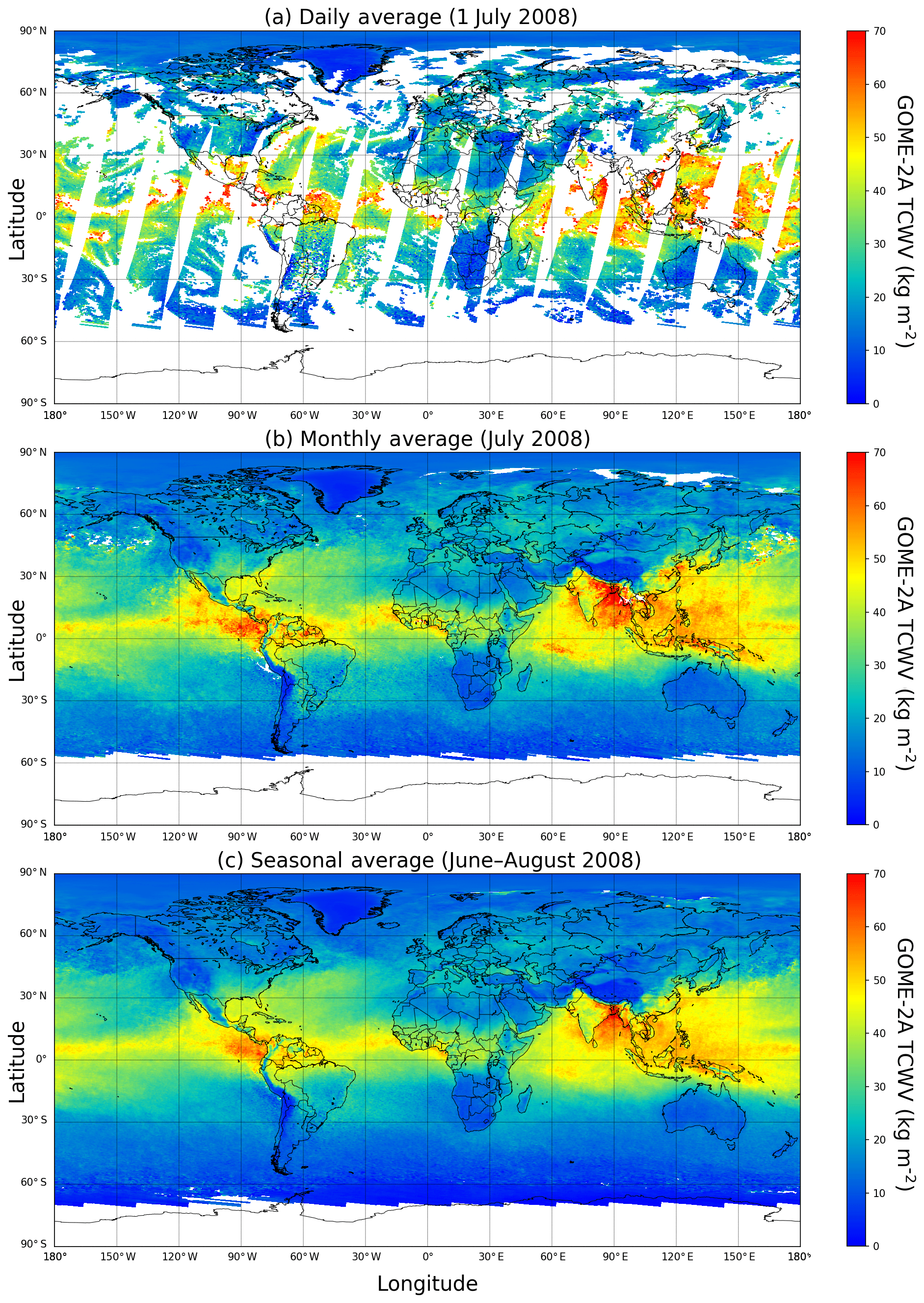
Figure 6 (a) Daily (1 July 2008), (b) monthly (July 2008) and (c) seasonal (June–August 2008) average of GOME-2A observations of TCWV.

3.2 Comparison methods

In this study, water vapor columns retrieved from GOME-2 observations in the blue band are compared to ground-based sun photometer and radiosonde measurements. As the satellite, sun photometer and radiosonde data are different in spatial and temporal resolution and coverage, only coinciding data are used in the comparison. The criteria used to select coinciding data are that the (1) satellite data are selected so that the center coordinate of the satellite pixel is within 50 km of the sun photometer or radiosonde site, and the (2) sun photometer or radiosonde data are selected around the satellite overpass time so that the time difference between the satellite and ground observations is less than 2 h. Subsequently, satellite, sun photometer and radiosonde measurements are averaged to daily data for comparison. As the sun photometer only provides data under clear-sky conditions, satellite data are filtered for intensity-weighted cloud fractions smaller than 0.5 for consistency. Daily averaged GOME-2 data are used for the comparison to sun photometer and radiosonde measurements.

4 Results

In this section, we present validation studies of GOME-2 TCWV retrieved in the blue spectral range. Our retrieval results are compared to the GOME-2 operational water vapor product which is derived in the red spectral band. In addition, the new data set is validated against ground-based sun photometer observations and radiosonde measurements.

4.1 Comparison to the GOME-2 operational product

4.1.1 Spatial distribution comparison

Figure 7a and d show the monthly average spatial distribution of TCWV retrieved from GOME-2A observations in the blue spectral band for January and July 2018. These months are chosen as examples for winter and summer. TCWV from the GOME-2 operational products are shown in Fig. 7b and e for comparison. Both data sets are gridded and filtered in the same way as described in Sect. 3.1.13. Missing data over the Tibetan Plateau and Andes mountains are due to no valid data being available over high-altitude areas in the operational product, while missing data over other smaller regions are mainly related to cloud filtering. The differences between the two data sets are plotted in Fig. 7c and f. Both data sets show very similar spatial patterns, with higher water vapor columns over the tropics and lower values at upper latitudes. The blue band retrieval shows significantly higher water vapor columns over west Africa (∼5 kg m⁻²), India (∼7 kg m⁻²) and the Southeast Asia Peninsula (∼6 kg m⁻²) during summertime in the Northern Hemisphere. In addition, the blue retrieval shows a small negative bias of about 0.5 kg m⁻² over oceans in the tropics.

Figure 7 Monthly average TCWV derived from the GOME-2A observations. Panels (a) and (d) show data from the blue band retrieval, panels (b) and (e) show data from the GOME-2 operational product (red band), and panels (c) and (f) show the differences between the two data sets. Panels (a–c) show the data from January 2018, while panels (d–f) show the data from July 2018.

4.1.2 Zonal average, correlation and bias

The water vapor columns derived from the blue band and the operational retrieval are sorted by their measurement latitudes and are plotted in Fig. 8a and c. Data from January and July of 2018 are shown. The retrieval in the blue spectral band show good zonal agreement with the operational product in both winter and summer. The 1σ standard deviation variation ranges of both data sets overlap with each other, indicating that both data sets capture similar spatial variations of water vapor columns. A direct comparison of individual measurements from both data sets is shown in Fig. 8b and d. The two data sets show very good agreement with Pearson correlation coefficients (R) ranging from 0.91 to 0.94. The correlation is slightly better during winter (January) in the Northern Hemisphere. The mean bias between the blue band retrieval and the operational product is 0.12 kg m⁻² in January 2018 and −0.08 kg m⁻² in July 2018.

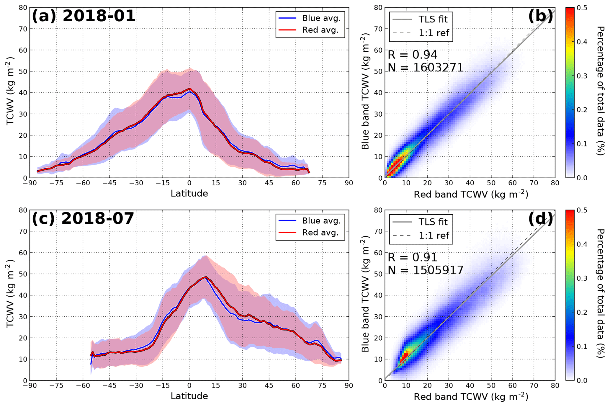
Figure 8 Comparison of TCWV from the blue retrieval and operational algorithm. (a) Zonal and (b) direct comparison in January 2018. Panels (c) and (d) are the same as panels (a) and (b) for July 2018. The shadings in the zonal average plots indicate the 1σ standard deviation variation range. The color code of the scatterplots indicates the relative portion of total measurement pixels. Individual GOME-2A measurements are used in the comparison.

Figure 9 shows the monthly zonal averaged TCWV derived from GOME-2A measurements for 11 years from 2008 to 2018. Both the blue retrieval and operational data sets are shown. Water vapor columns from both data sets show very similar zonal distribution patterns. Compared to the operational product, the blue retrieval before 2015 shows slightly lower water vapor columns over the tropics and higher values in the upper latitudes, resulting in a small wet bias of ∼1 kg m⁻². The wet bias is greatly reduced to less than 0.1 kg m⁻² after 2015.

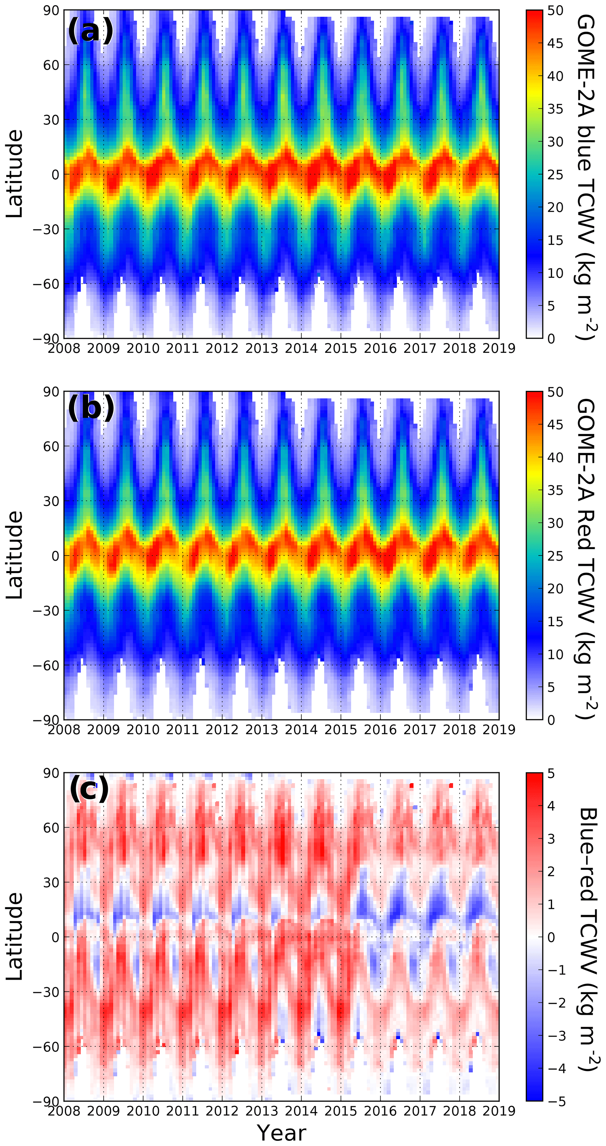
Figure 9 Monthly zonal average of TCWV from GOME-2A observations in the (a) blue and (b) red spectral bands. The differences between the two data sets are shown in (c). Data over 11 years, from 2008 to 2018, are shown.

Figure 10 shows the time series of the correlation and mean bias between the blue retrieval and the operational algorithm. Data from 2008 to 2018 are shown. The correlation between the two data sets is, in general, very good, with the Pearson correlation coefficient (R) ranging from 0.90 to 0.96. The correlation between both data sets is generally higher in winter in the Northern Hemisphere and lower during summer. A significant overestimation of TCWV is observed for measurements from 2008 to 2015. The bias between the two data sets is greatly improved after 2015.

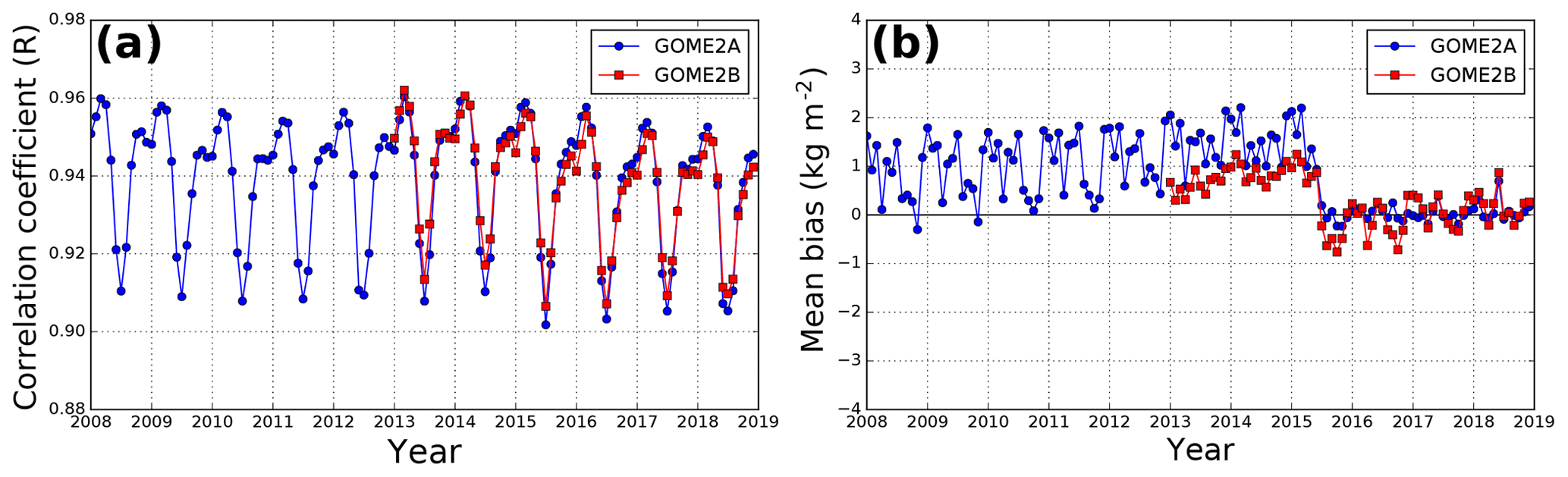
Figure 10 Time series of a Pearson correlation coefficient between water vapor columns from the blue band retrieval and operational algorithm is shown in (a). Panel (b) shows the mean bias between the two data sets. Both GOME-2A and GOME-2B data are shown. Individual measurements are used in the calculation of correlation coefficient and mean bias.

In addition, we have compared the TCWV measured by both GOME-2A and GOME-2B to investigate the cross-sensors consistency. The mean water vapor column retrieved from GOME-2A observations from 2013 to 2014 is 20.72 kg m⁻², while GOME-2B observations show a similar value of 20.91 kg m⁻². The bias between the two GOME-2 sensors before the level 1B data update is ∼1 %. The mean water vapor column retrieved from GOME-2A observations from 2016 to 2018 is 20.53 kg m⁻², while GOME-2B shows a very similar value of 20.87 kg m⁻². The bias of the water vapor column retrieved in the blue band between the two sensors remains at a similar level (<2 %) after the update of level 1B data. On the other hand, the bias of the water vapor column retrieved in the red band between GOME-2A and GOME-2B lies between 3 % and 4 % for data before and after the level 1B update.

4.1.3 Long-term variations

Figure 11a and c show the time series of annual mean TCWV derived from GOME-2A and GOME-2B observations. The rate of change in TCWV calculated from GOME-2A and GOME-2B measurements is also shown in Fig. 11b and d, respectively. Both GOME-2A blue and red band measurements, in general, suggest a slightly increasing trend. The interannual variation of TCWV captured by the blue band retrieval and operational product agree well with each other, except for the year of 2015 when the level 1B processor was updated. The averaged rate of change in TCWV derived from GOME-2A by the blue retrieval is about 0.12 kg m⁻² yr⁻¹, while a higher increasing rate of 0.19 kg m⁻² yr⁻¹ is observed in the red band. If we remove the year of 2015 from the analysis, the average rate of change calculated from the blue retrieval increases from 0.12 to 0.17 kg m⁻² yr⁻¹ and agrees better with the operational product. A similar increasing rate can also be observed by the GOME-2B sensor, with an averaged rate of change derived from the blue and red band of 0.12 and 0.21 kg m⁻² yr⁻¹, respectively. If the year of 2015 is removed from the trend analysis, then the increasing rate derived from the blue band would increase to 0.26 kg m⁻² yr⁻¹. Although the increase rate of 0.12–0.26 kg m⁻² yr⁻¹ is not significant compared to the typical temporal variation of water vapor (∼2.5 kg m⁻²), the trend of the atmospheric water vapor content is a major concern for climate change and has to be cross validated with other observations and model simulations to investigate the causes and the impacts to the climate system. A further discussion of this topic is, however, beyond the scope of this study.

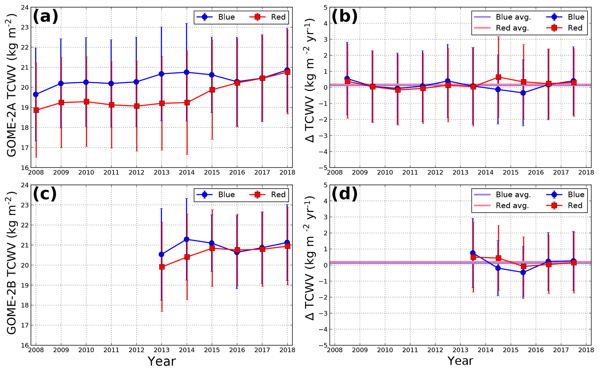
Figure 11 Time series of annual average of TCWV retrieved from (a) GOME-2A and (c) GOME-2B in blue (blue curves) and red (red curve) spectral bands. The rate of change in TCWV derived from (b) GOME-2A and (d) GOME-2B is also shown. The purple and pink lines indicate the average rate of change derived from the blue and red band measurements, respectively. The error bars indicate the 1σ standard deviation of the annual variation.

4.2 Comparison to sun photometer data

Figure 12a and b show the scatterplot of GOME-2A and GOME-2B measurements of TCWV against sun photometer measurements. The selection criteria for data sets used in the comparison are presented in Sect. 3.2. Co-located daily averaged data are used in the comparison. The sun photometer and GOME-2 measurements of TCWV agree well with each other. The Pearson correlation coefficient (R) is 0.91 and 0.89 for GOME-2A and GOME-2B observations, respectively. The slope of the total least squares regression line for the GOME-2A comparison is 0.99, with an offset of 0.84 kg m⁻². The analysis of GOME-2B data shows a similar result with a slope of 1.00 and offset of 1.03 kg m⁻². The mean bias between sun photometer data and observations from GOME-2A and GOME-2B is 0.78 and 1.09 kg m⁻², respectively.

Figure 12 Comparison of the TCWV, measured by the sun photometer, to GOME-2A is shown in (a), while the comparison to GOME-2B is shown in (b). Co-located daily averaged data are used in the comparison.

Figure 13 shows the statistic of the differences between the sun photometer and GOME-2 measurements of TCWV. Data are sorted by year, month and latitude to investigate the spatiotemporal agreement between the two data sets. The interannual variation analysis shows a small positive bias of 1–2 kg m⁻² for both GOME-2A and GOME-2B observations before 2015. The overestimation is significantly improved after the update of level 1B data in 2015. The discrepancies between GOME-2 and sun photometer show a larger variation range in the summer months in the Northern Hemisphere. In addition, a larger variation of discrepancies is also observed over the tropics compared to upper latitudes.

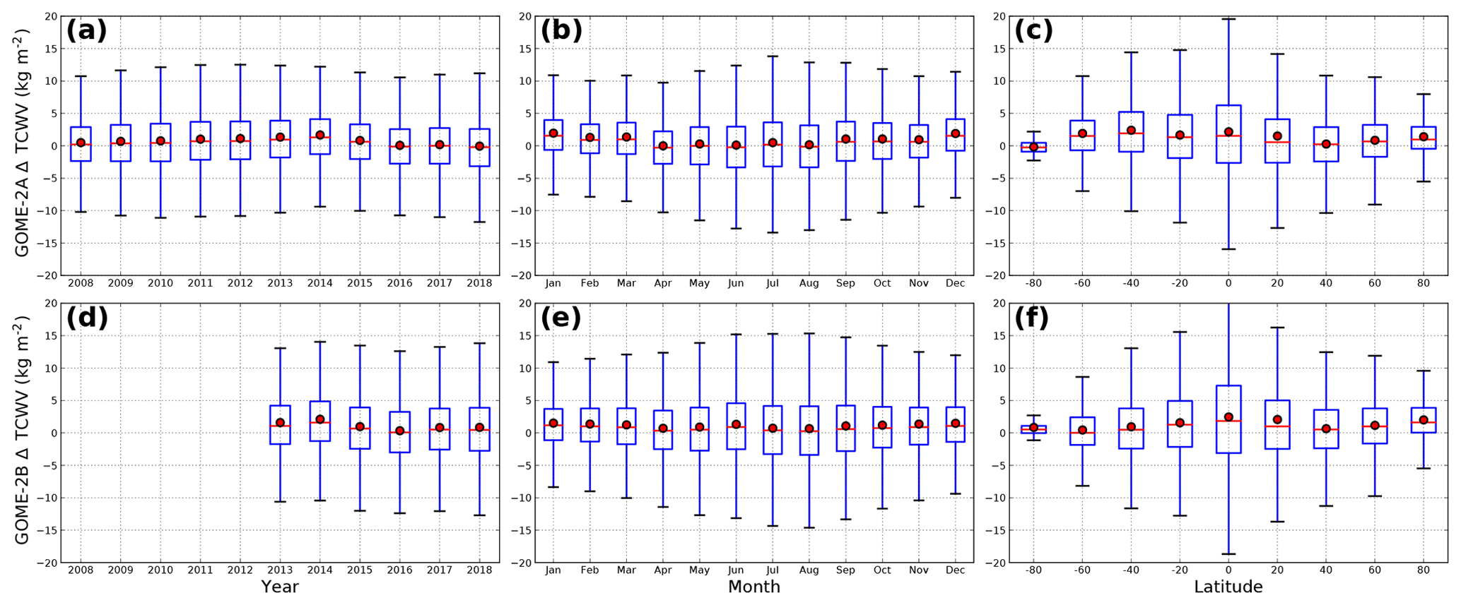
Figure 13 Comparison between sun photometer and GOME-2A observations. Panels (a–c) show GOME-2A data and panels (d–f) show GOME-2B data. Data are sorted by year in (a) and (d), month in (b) and (e), and latitude in (c) and (f).

4.3 Comparison to radiosonde measurements

The scatterplots of the radiosonde TCWV measurements compared to the GOME-2A and GOME-2B measurements are shown in Fig. 14. The selection criteria for the data sets used in the comparison are presented in Sect. 3.2. Co-located daily averaged data are used in the comparison. Both GOME-2A and GOME-2B measurements are consistent with the radiosonde measurements with the Pearson correlation coefficient (R) of 0.92 and 0.91, respectively. The slope of the total least squares regression line for the GOME-2A comparison is 0.99, with an offset of 1.33 kg m⁻². A similar agreement can also be obtained from GOME-2B observations, with a slope of 1.02 and an offset of 0.42 kg m⁻². The mean bias between radiosonde data and observations from GOME-2A and GOME-2B are 1.20 and 0.88 kg m⁻², respectively.

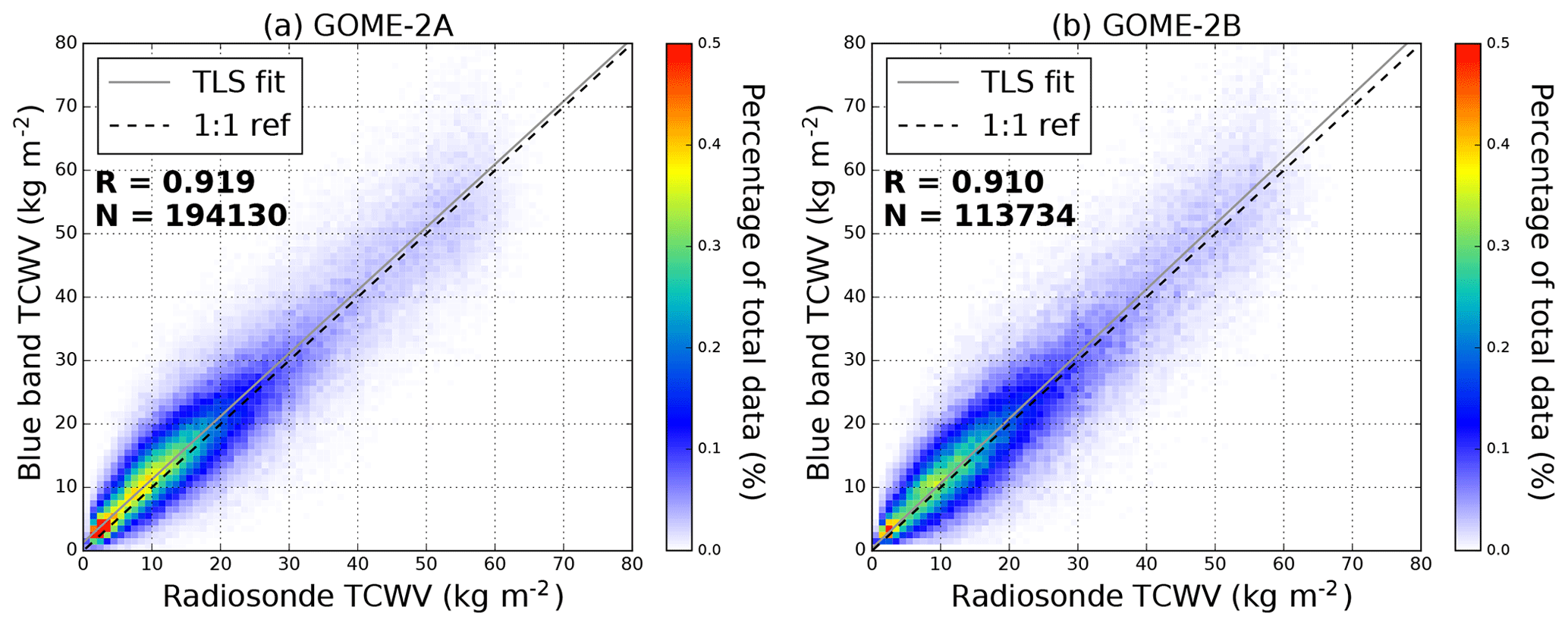
Figure 14 Comparison of radiosonde measurements of TCWV to GOME-2A is shown in (a), while the comparison to GOME-2B observations is shown in (b). Co-located data are used in the comparison.

Figure 15 shows the statistic of the differences between radiosonde and GOME-2 measurements of TCWV. Data are sorted by year, month and latitude to investigate the spatiotemporal agreement between the two data sets. Similar to the sun photometer comparison result, the GOME-2 data overestimated the water vapor columns by ∼1 kg m⁻² before 2015. The monthly pattern also shows a larger variation range in summer months in the Northern Hemisphere. The discrepancies between GOME-2 and radiosonde also vary in a larger range over the tropics and are lower at upper latitudes.

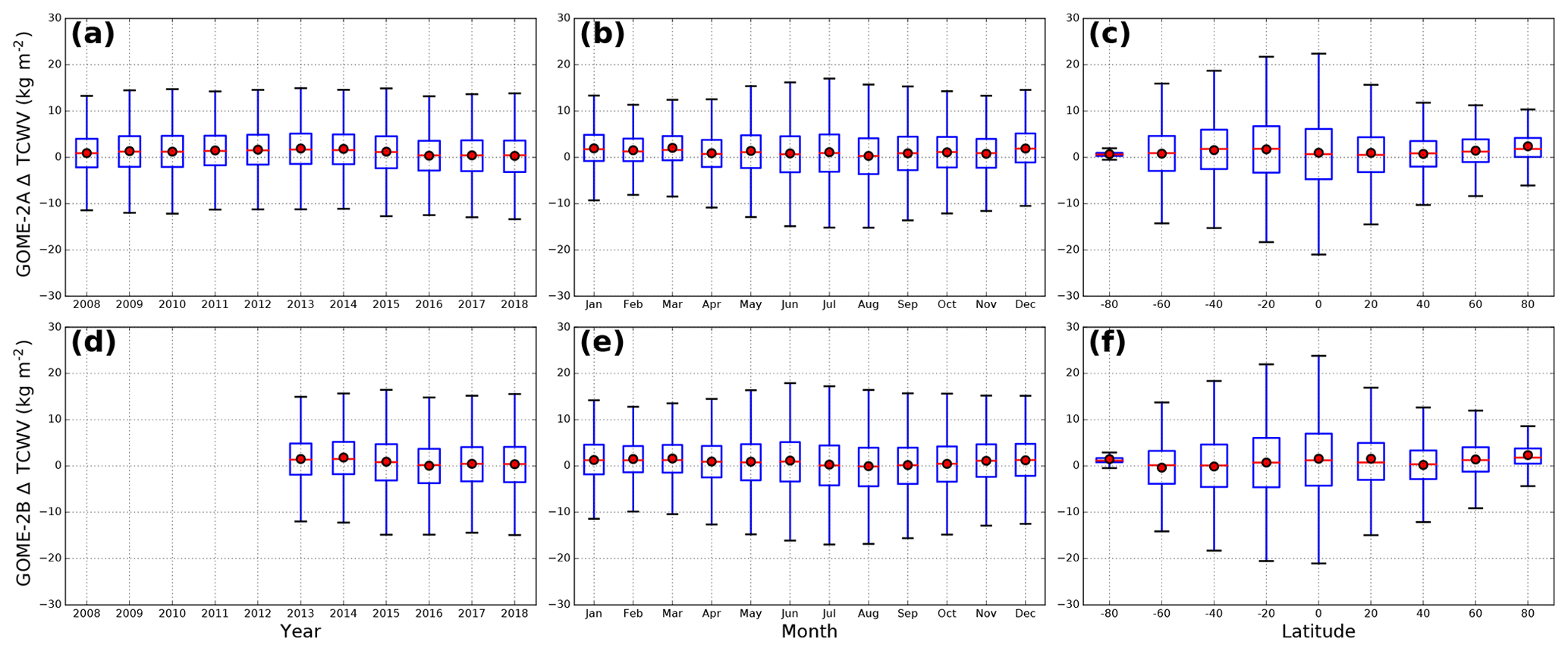
Figure 15 Comparison between radiosonde and GOME-2A observations. Panels (a–c) show GOME-2A data and panels (d–f) show GOME-2B data. Data are sorted by year in (a) and (d), month in (b) and (e), and latitude in (c) and (f)

5 Discussion

5.1 Comparison to the GOME-2 operational product

5.1.1 Spatial distribution comparison

The spatial distribution of water vapor from the blue band and operational retrieval shows good consistency. However, the blue band retrieval shows significantly higher values over west Africa, India and Southeast Asia Peninsula and slightly lower values over oceans in the tropics in July. A previous study reported that the operational GOME-2 product is underestimating water vapor columns over land and overestimating them over oceans in the tropics (Grossi et al., 2015). The differences between the two data sets indicate that the blue band retrieval improved the bias over these areas.

Overestimation of TCWV can also be observed over South America in both summer and winter. The discrepancies are likely related to the uncertainties of Lambertian assumption of surface albedo over vegetation. The bidirectional reflectance distribution function (BRDF) effect has been reported to have significant impacts on the retrieval of cloud and trace gas over forested scenes (Lorente et al., 2018). The uncertainty of the cloud product due to the BRDF effect over vegetation also indirectly affects the water vapor retrieval. In this study, the Lambertian surface assumption is used in the water vapor retrieval to be consistent with the cloud product. Using the Lambertian surface assumption over areas covered by vegetation probably leads to overestimation of the water vapor columns. In addition, interannual variation of surface assumption also affects the retrieval results. Sütterlin et al. (2016) analyzed the Advanced Very High Resolution Radiometer (AVHRR) BRDF product from 1990 to 2014, and the result shows that the interannual variability of the land surface albedo is in general less than 0.01 for snow-free vegetation cover but possibly larger than 0.06 for regions covered by snow or ice. We performed a sensitivity analysis to quantify the uncertainty TCWV caused by the interannual variation of albedo by using the numbers provided in Sütterlin et al. (2016). The result shows that the uncertainty of TCWV due to interannual variations of surface albedo is, in general, <2 %, while the uncertainty increased to ∼9 % for areas covered by snow and ice. In the future, we plan to update the surface albedo retrieval to account for the temporal variation in albedo and the BRDF effect (Loyola et al., 2020). The updated surface albedo product will also improve the accuracy of cloud retrieval and further improve the water vapor retrieval.

5.1.2 Zonal average, correlation and bias

Compared to the operational product, the blue retrieval is overestimating the water vapor columns at upper latitudes and underestimating in the tropics and resulting a small overestimation (∼5 %) for measurements before 2015. Water vapor columns retrieved at the blue band are, in general, reduced in both tropical regions and high latitudes after 2015. As a result, the difference between the two data sets becomes smaller at higher latitudes, while a slightly stronger underestimation is observed over the tropics. This change is likely related to the level 1B data processing being switched from version 6.0 to version 6.1 on 25 June 2015; this affects the blue band but not the red band. Although the uncertainty caused by the contaminated level 1B data is small and well covered by the assumed uncertainties, the bias is still significant when averaging large numbers of data for climate studies. The overall bias between the two GOME-2A data sets is reduced from 1.14 kg m⁻² before the update (2008–2014) to 0.05 kg m⁻² after the update (2016–2018). A similar effect is also observed in the GOME-2B water vapor retrieval. The mean bias between the GOME-2B blue retrieval and operational product is ∼0.75 kg m⁻² before the update (2013–2014), and it is reduced to ∼0.05 kg m⁻² after the update (2016–2018). The result indicates that reprocessing of level 1B data before 2015 is necessary to produce a reliable TCWV data set.

A previous comparison of the GOME-2 operational water vapor product to radiosonde measurements shows that the operational product is, on average, underestimating water vapor columns over land by 1.0 kg m⁻² and overestimating over ocean by 1.5 kg m⁻² (Kalakoski et al., 2016). After the update of level 1B data in 2015, the blue retrieval is reporting slightly higher water vapor columns than the operational product at upper latitudes, and lower values are observed over the tropics.

5.2 Comparison to sun photometer data

The small positive offsets between GOME-2 and sun photometer measurements indicate that the blue band retrieval slightly overestimates the TCWV. On the other hand, the sun photometer data have been reported to underestimate TCWV by 6 %–9 % compared to GPS data (Pérez-Ramírez et al., 2014). In addition, the GOME-2 to sun photometer comparison also includes data before 2015, where the level 1B data are contaminated and enhance the TCWV by up to 2 kg m⁻². If we only consider data taken after 2015 in the comparison, the bias of GOME-2A would reduce from 0.78 to 0.09 kg m⁻², and the bias of GOME-2B would also reduce from 1.09 to 0.64 kg m⁻². Considering all the uncertainties in the sun photometer (6 %–9 %) and GOME-2 (∼20 %) measurements, the small discrepancies between the two data sets are considered reasonable.

The analysis of bias between GOME-2 and sun photometer measurements shows a larger variation during summer months of the Northern Hemisphere. This is partly related to the geolocation distribution of the sun photometer stations. Most of the stations are situated in the Northern Hemisphere and result in a larger number of valid measurements and variations in summer. In addition, both GOME-2A and GOME-2B are slightly overestimating the water vapor columns by ∼1 kg m⁻² during winter months, i.e., January, February and December. Our observations are consistent with the previous radiosonde comparison study (Antón et al., 2015). The reason for larger discrepancies during winter is likely related to the variation in surface albedo (snow and ice cover). The zonal variation analysis shows larger variations in the tropics, while the variations are much smaller at higher latitudes. The uncertainty of TCWV derived from satellite observations is strongly related to the air mass factor uncertainty. As the air mass factor is a multiplication term and there is larger amount of water vapor over the tropics, this results in a larger absolute uncertainty.

5.3 Comparison to radiosonde measurements

The small overestimation of water vapor columns by GOME-2 compared to radiosonde measurements is partly related to the level 1B data issued before 2015. If we only consider data taken after 2015 in the comparison, the overestimation of GOME-2A is reduced from 1.20 to 0.36 kg m⁻², and the bias of GOME-2B is also reduced from 0.88 to 0.31 kg m⁻². In addition, the radiosonde measurements stop at a certain altitude and do not cover the entire atmosphere, which may slightly underestimate the total column. The discrepancy between the satellite and radiosonde measurements is below 5 %, which is well within the uncertainties of radiosonde measurements reported from previous studies (Wang and Zhang, 2008; Van Malderen et al., 2014). A previous comparison of the GOME-2 operational product to radiosonde data shows a dry bias of 4 %–11 % (Antón et al., 2015). In contrast, the new retrieval results show a much more reasonable wet bias of <2 %. Considering the uncertainty radiosonde and the GOME-2 retrieval, the two data sets are in good agreement with each other.

6 Conclusions

In this work, we have developed a water vapor retrieval algorithm in the visible blue band of 427.7–455 nm, providing an alternative solution for satellite sensors that do not cover the red band where TCWV is typically retrieved. The major advantage of the new water vapor retrieval algorithm is that it does not rely on a priori information from a chemistry transport model. This improvement makes the satellite product independent from model simulations and avoids model errors propagating to the measurement, making the data more suitable for climate studies.

The developed TCWV retrieval has been successfully applied to GOME-2. Water vapor columns retrieved in the blue band show very good spatiotemporal consistency with the operation product, sun photometer and radiosonde measurements. However, reprocessing of GOME-2 level 1B data before 2015 is necessary to produce a reliable climate record. The blue band retrieval results are consistent between GOME-2A and GOME-2B, with discrepancies of less than 2 %. The retrieval is feasible enough to be applied to former, current and forthcoming UV and Vis satellite sensors to create an independent water vapor climate data record starting from 1995 and continuing for the next two decades.