Cloud-top pressure retrieval with DSCOVR EPIC oxygen A- and B-band observations

An analytic transfer inverse model for Earth Polychromatic Imaging Camera (EPIC) observations is proposed to retrieve the cloud-top pressure (CTP) with the consideration of in-cloud photon penetration. In this model, an analytic equation was developed to represent the reflection at the top of the atmosphere from above cloud, in cloud, and below cloud. The coefficients of this analytic equation can be derived from a series of EPIC simulations under different atmospheric conditions using a nonlinear regression algorithm. With estimated cloud pressure thickness, the CTP can be retrieved from EPIC observation data by solving the analytic equation. To simulate the EPIC measurements, a program package using the double-k approach was developed. Compared to line-by-line calculation, this approach can calculate high-accuracy results with a 100-fold computation time reduction. During the retrieval processes, two kinds of retrieval results, i.e., baseline CTP and retrieved CTP, are provided. The baseline CTP is derived without considering in-cloud photon penetration, and the retrieved CTP is derived by solving the analytic equation, taking into consideration in-cloud and below-cloud interactions. The retrieved CTPs for the oxygen A and B bands are smaller than their related baseline CTP. At the same time, both baseline CTP and retrieved CTP at the oxygen B band are larger than those at the oxygen A band. Compared to the difference in baseline CTP between the B band and A band, the difference in retrieved CTP between these two bands is generally reduced. Out of around 10 000 cases, in retrieved CTP between the A and B bands we found an average bias of 93 mb with a standard deviation of 81 mb. The cloud layer top pressure from Cloud–Aerosol Lidar and Infrared Pathfinder Satellite Observations (CALIPSO) measurements is used for validation. Under single-layer cloud situations, the retrieved CTPs for the oxygen A band agree well with the CTPs from CALIPSO, the mean difference of which within 5 mb in the case study. Under multiple-layer cloud situations, the CTPs derived from EPIC measurements may be larger than the CTPs of high-level thin clouds due to the effect of photon penetration.

1 Introduction

The Deep-Space Climate Observatory (DSCOVR) satellite is an observation platform orbiting within the first Sun–Earth Lagrange point (L1), 1.5 million km from the Earth, carrying a suite of instruments oriented both earthward and sunward. One of the earthward instruments is the Earth Polychromatic Imaging Camera (EPIC), which can take images of the Earth with a spatial resolution of 10 km at nadir. EPIC continuously monitors the entire sunlit Earth for backscatter, with a nearly constant scattering angle between 168.5 and 175.5^∘ from sunrise to sunset with 10 narrowband filters: 317, 325, 340, 388, 443, 552, 680, 688, 764, and 779 nm (Marshak et al., 2018). Of the 10 narrowband channels, there are two oxygen absorption and reference pairs, 764 nm versus 779.5 nm and 680 nm versus 687.75 nm, for the oxygen A and B bands. The cloud-top pressure (CTP) or cloud-top height (CTH) is an important cloud property for climate and weather studies. Based on differential oxygen absorption, both EPIC oxygen A-band and B-band pairs can be used to retrieve CTP. It is worth noting that although CTP and CTH reference the same characteristic of clouds, the conversion between the two depends on the related atmospheric profile.

Although the theory of using oxygen absorption bands to retrieve CTP was proposed decades ago (Yamamoto and Wark, 1961), it is still very challenging to perform retrievals accurately due to the complicated in-cloud penetration effect (Yang et al., 2019, 2013; Davis et al., 2018a, b; Richardson and Stephens, 2018; Loyola et al., 2018; Lelli et al., 2014, 2012; Schuessler et al., 2013; Ferlay et al., 2010; Rozanov and Kokhanovsky, 2004; Kokhanovsky and Rozanov, 2004; Daniel et al., 2003; Koelemeijer et al., 2001; Kuze and Chance, 1994; O'Brien and Mitchell, 1992; Fischer and Grassl, 1991). To estimate the CTP from satellite measurements, many approaches have been designed to retrieve cloud effective top pressures without considering in-cloud photon penetration. These approaches do not consider light penetrating cloud, and therefore the derived CTH is lower than the cloud top, and the effective top pressure is higher than CTP. In the meantime, to improve the retrieval accuracy of CTP, various techniques have been applied to retrieval methods with in-cloud photon penetration. For example, Kokhanovsky and Rozanov (2004) proposed a simple semi-analytical model for the calculation of the top-of-atmosphere (TOA) reflectance of an underlying surface–atmosphere system accounting for both aerosol and cloud scattering. Based on the work of Kokhanovsky and Rozanov (2004), Rozanov and Kokhanovsky (2004) developed an asymptotic algorithm for the CTH and the geometrical thickness determination using measurements of the cloud reflection function. This retrieval method was applied by Lelli et al. (2012, 2014) to derive CTH using measurements from the GOME instrument onboard the ESA ERS-2 space platform.

Currently, based on the measurements of DSCOVR EPIC, the Atmospheric Science Data Center (ASDC) at the National Aeronautics and Space Administration (NASA) Langley Research Center archives both calibrated EPIC reflectance ratio data and processed Level 2 cloud retrieval products, including cloud cover, cloud optical depth (COD), and cloud effective top pressure at oxygen A and B bands (Yang et al., 2019; Holdaway and Yang, 2016; Meyer et al., 2016). By using EPIC reflectance ratio data at oxygen A-band and B-band absorption to reference channels, Yang et al. (2013) developed a method to retrieve CTH and cloud geometrical thickness simultaneously for a fully cloudy scene over ocean surface. First, their method calculates cloud centroid heights for both A- and B-band channels using the ratios between the reflectance of the absorption and reference channels, then derives the CTH and the cloud geometrical thickness from the two-dimensional lookup tables that relate the sum and the difference between the retrieved centroid heights for the A and B bands to the CTH and the cloud geometrical thickness. The difference in the O₂ A- and B-band cloud centroid heights results from the different penetration depths of the two bands. Compared to the cloud height variability, the penetration depth differences are much smaller, and the retrieval accuracy from this method can be affected by instrument noise (Davis et al., 2018a, b).

In this paper, to address the issue of in-cloud penetration, we propose an analytic method to retrieve the CTP by using DSCOVR EPIC oxygen A- and B-band observations. This analytical method adopts ideas of the semi-analytical model (Kokhanovsky and Rozanov, 2004; Rozanov and Kokhanovsky, 2004) with a quadratic EPIC analytic radiative transfer equation to analyze the radiative transfer in oxygen A- and B-band channels. The structure of this paper is as follows: Sect. 2 describes the theory and methods, which includes several subsections, i.e., the introduction of DSCOVR EPIC oxygen A- and B-band filters, the theory of CTP retrieval based on EPIC oxygen A- and B-band observations, and the detailed retrieval algorithm. Section 3 describes the application and validation of the CTP retrieval method, which also includes several subsections, i.e., case studies of CTP retrieval, validation of the retrieval method, and retrieval of global observation. Section 4 states the conclusions of this study.

2 Theory and methods

2.1 DSCOVR EPIC oxygen A- and B-band filters

EPIC filters at 764 and 779 nm cover the oxygen A-band absorption and reference bands, respectively (Fig. 1a). The high-resolution absorption optical depth spectrum at the oxygen A band and B band is calculated by the Line-By-Line Radiative Transfer Model (LBLRTM; Clough et al., 2005) with the HITRAN 2016 database (Gordon et al., 2017) for the US standard atmosphere. In this wavelength range, the O₃ absorption is very weak (O₃ optical depth <0.003) and there are no other gas absorptions. The background aerosol and Rayleigh scattering optical depth vary smoothly within the A-band range; the differences between in-band and the reference band are negligible at nominal EPIC response functions. EPIC filters at 688 and 680 nm cover the oxygen B-band absorption and reference band, respectively (Fig. 1b). Compared to the oxygen A band, O₃ absorption is slightly stronger in the oxygen B-band range, with an O₃ optical depth around 0.01. Any water vapor absorption in the B-band range is negligible. In the standard atmospheric model, from the oxygen B-band reference band to the absorption band, the O₃ absorption and Rayleigh scattering optical depth decreased by approximately 0.002 and 0.002, respectively. This may have some impacts on the CTP retrieval from the oxygen B band (more discussion in later sections). It is worth noting that for EPIC measurements at both oxygen A and B bands, the surface influence cannot be ignored. For example, in snow- or ice-covered area the surface albedo is high; in plant-covered area, the surface albedo changes substantially between the oxygen A band and B band due to the impact of the spectral red edge (Seager et al., 2005).

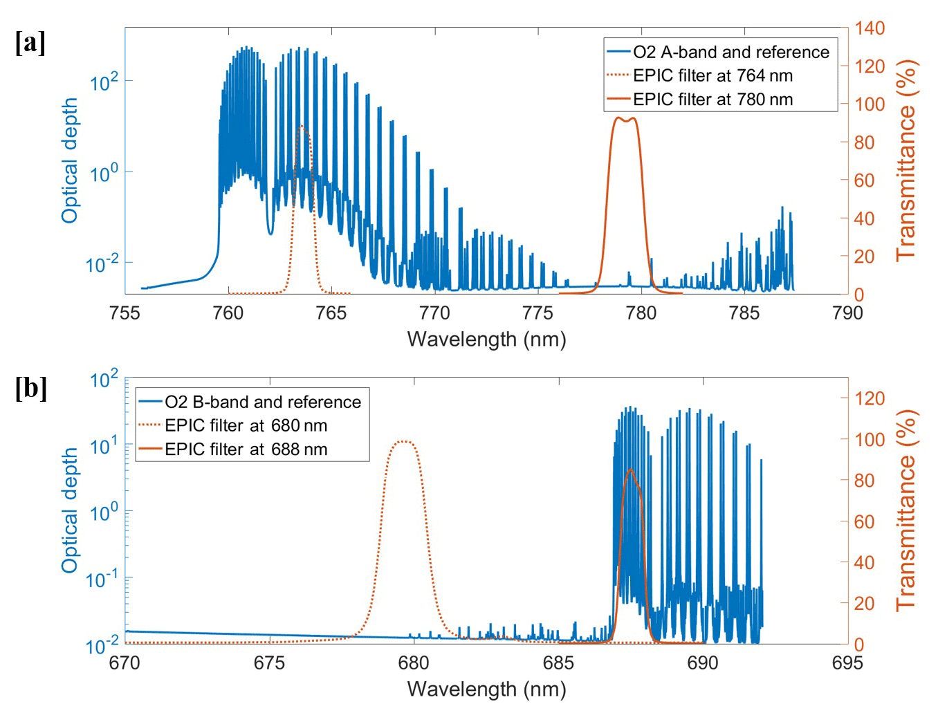
Figure 1 High-resolution calculated absorption optical depth spectrum at the oxygen A band (a) and B band (b) with DSCOVR EPIC oxygen A- and B-band in-band and reference filters. Here the absorption optical depth spectrum is calculated by the LBLRTM model with the HITRAN 2016 database for the US standard atmosphere.

In general, if we use the pair of oxygen A and B absorption and reference bands together, the impact of other absorption lines, background Rayleigh scattering, and aerosol optical depth is very limited. At the same time, as a well-mixed major atmospheric component, the vertical distribution of oxygen in the atmosphere, is very stable under varying atmospheric conditions. Thus, we can use the ratio of reflected radiance (or reflectance) at the TOA of oxygen absorption to reference bands (i.e., R₇₆₄ and R₇₇₉, R₆₈₈, and R₆₈₀) to study the photon path length distribution and derive cloud information. Also, compared to any specific EPIC oxygen absorption bands (i.e., R₇₆₄ and R₆₈₈), the ratios of absorption to reference channels (i.e., R₇₆₄∕R₇₇₉ and R₆₈₈∕R₆₈₀) are less impacted by instrument calibration and other measurement error. This can be explained by the following reasons: first, the EPIC measurements at the oxygen A and B absorption and reference bands share the same sensor and optical system, so when calculating the ratios, some preprocessing calibration errors can be reduced. Second, to calculate R₇₆₄ and R₆₈₈, the ratio of lunar reflectance at neighboring channels (i.e., F(764, 779) and F(688, 680)) to the calibration factors of the oxygen A and B reference bands (i.e., K₇₇₉ and K₆₈₀) are used (Geogdzhayev and Marshak, 2018; Marshak et al., 2018). Therefore, the accuracy of R₇₆₄ and R₆₈₈ is determined by the stability of F(764, 779) and F(688, 680) and the accuracy of K₇₇₉ and K₆₈₀ together. But the accuracy of the absorption to reference ratios is only determined by the stability of F(764, 779) and F(688, 680).

2.2 Theory of CTP retrieval based on EPIC oxygen A- and B-band observation

In our study, we tried two methods to retrieve the CTP based on EPIC oxygen A-band and B-band measurements: (1) build a lookup table (LUT) for various atmospheric conditions and perform the retrieval by searching the LUT; (2) develop an analytic transfer inverse model for EPIC observations and calculate the related coefficients based on a series of simulated values, then use this analytic transfer inverse model to retrieve the CTP. In this paper, we mainly focus on the second method.

2.2.1 Method 1: LUT-based approach

One commonly used method of retrieval for satellite observation is through the building and usage of LUTs (Loyola et al., 2018, Gastellu-Etchegorry and Esteve, 2003). The LUT-based approach can be fast because the most computationally expensive part of the inversion procedure is completed before the retrieval itself. For DSCOVR EPIC observations, we can build LUTs by simulating EPIC measurements under various atmospheric conditions, such as different surface albedo, solar zenith and viewing angles, COD, CTP, and cloud pressure thickness. Comparing the related simulated reflectance at the oxygen absorption and reference bands, we can obtain two LUTs for the reflectance ratios of absorption to reference at the EPIC oxygen A band and B band, respectively, which can be used for the CTP retrieval. Detailed information on the simulated reflectance ratio of absorption to reference is stated in Sect. 2.3.3.

During the retrieval process, the EPIC measurements (e.g., reflectance at oxygen A and B bands) with related solar zenith and viewing angles can be obtained from the EPIC Level 1B data; COD information (retrieved from other EPIC channels) can be obtained from EPIC Level 2 data. At the same time, we can get surface albedo from Global Ozone Monitoring Experiment 2 (GOME-2) surface Lambertian-equivalent reflectivity (LER) data (Tilstra et al., 2017). At this point the CTP and cloud pressure thickness are the only unknown variables. The cloud pressure thickness or the cloud vertical distribution has a substantial impact on the accuracy of the CTP retrievals (Carbajal Henken et al., 2015; Fischer and Grassl, 1991; Rozanov and Kokhanovsky, 2004; Preusker and Lindstrot, 2009). In this study, the cloud pressure thickness is used as an input parameter to retrieve the CTP. However, no related accurate cloud pressure thickness is currently provided by other satellite sensors. To constrain the error from the estimation of cloud pressure thickness, we related it to the cloud optical thickness. It is reasonable because clouds with higher optical thickness normally have higher values of pressure thickness. To explore the correlation between cloud pressure thickness and cloud optical thickness, we use the related cloud data from the Modern-Era Retrospective analysis for Research and Applications version 2 (MERRA-2; Gelaro et al., 2017), which is a NASA atmospheric reanalysis for the satellite era using the Goddard Earth Observing System Model version 5 (GEOS-5) with Atmospheric Data Assimilation System (ADAS). Based on statistical analysis of 1-year single-layer liquid water clouds over an oceanic region (23.20^∘ S, 170.86^∘ W; 2.11^∘ S, 144.14^∘ W) in 2017, we can get an equation for cloud pressure thickness approximation, i.e., cloud pressure thickness (mb) $=\mathrm{2.5}\times \text{COD}+\mathrm{23}$. The derived correlation coefficients are dependent on the case region and time selections. Due to the complexity of cloud vertical distribution, whatever the accuracy of the correlation coefficients is, the estimation will certainly bring in error.

With an estimated cloud pressure thickness, a multivariable LUT searching method can then be used to interpolate and obtain the CTP. It is worth noting that the reflectance ratio of absorption to reference can be seen as a function of surface albedo, solar zenith and viewing angles, COD, CTP, and cloud pressure thickness. Some atmospheric variables will have a nonlinear effect on the reflectance ratio. For example, the reflectance ratio is more sensitive to the variation of COD when COD is small. Overall, the reflectance ratio varies monotonically and smoothly with these variables (shown in Fig. 3). With a relatively high-resolution simulated table, we can use a localized linear interpolation method to estimate the proper values. Multiple interpolations are needed for this method to decrease the number of LUT dimensions, which will cost more time than the analytic transfer inverse model method. The retrieval error of this method is determined by the resolution of the LUT; i.e., the higher the resolution, the higher the retrieval accuracy. However, for multiple dimensional LUTs, the increase in resolution will increase the table size exponentially, which will increase computational cost substantially for the table building and inverse searching. Another possible method to increase the retrieval accuracy is using different interpolation methods. For example, if the value of LUT varies nonlinearly with a variable, using a high-order interpolation method may be better than using a linear interpolation method (Dannenberg, 1998).

2.2.2 Method 2: analytic transfer inverse model

For a long time, various efforts have been devoted to the study of radiative transfer in the atmosphere, including scattering, absorption, and emission (Chandrasekhar, 1960; Irvine, 1964; Ivanov and Gutshabash, 1974; van de Hulst, 1980, 2012; Ishimaru, 1999; Thomas and Stamnes, 2002; Davis and Marshak, 2002; Kokhanovsky et al., 2003; Marshak and Davis, 2005; Pandey et al., 2012). In this study, we develop an analytic radiative transfer equation to analyze the radiative transfer at the oxygen A and B bands. Through solving the analytic equation, we can retrieve the CTP information directly. The theory of CTP retrieval is similar for EPIC oxygen A-band and B-band observations. Here we use the oxygen A band as an example to study the radiative transfer model. For the oxygen A band, the photon path length distribution is capable of describing vital information related to a variety of cloud and atmospheric characteristics:

$$\begin{array}{}\text{(1)}& \begin{array}{rl}& I_{\mathit{\nu }}\left(\mathit{\mu },\mathit{\varphi };{\mathit{\mu }}_{\mathrm{0}},{\mathit{\varphi }}_{\mathrm{0}}\right)\\ & =I_{\mathrm{0}}\left(\mathit{\mu },\mathit{\varphi };{\mathit{\mu }}_{\mathrm{0}},{\mathit{\varphi }}_{\mathrm{0}}\right){\int }_{\mathrm{0}}^{\mathrm{\infty }}p\left(l,\mathit{\mu },\mathit{\varphi };{\mathit{\mu }}_{\mathrm{0}},{\mathit{\varphi }}_{\mathrm{0}}\right)e^{-{\mathit{\kappa }}_{\mathit{\nu }}l}\mathrm{d}l,\end{array}\end{array}$$

where p(l) is the photon path length distribution, κ_ν is the gaseous absorption coefficient at wavenumber v, $\mathit{\mu }=\cos \left(\mathit{\theta }\right),{\mathit{\mu }}_{\mathrm{0}}=\cos \left({\mathit{\theta }}_{\mathrm{0}}\right)$, (θ,ϕ) and (θ₀,ϕ₀) are zenith and azimuth angles for the solar and sensor view, respectively, and I₀ and I_ν are incident solar radiation and sensor-measured solar radiation, respectively.

When clouds exist, the incident solar radiation is reflected to TOA in three primary ways. First, incident solar radiation is reflected by the cloud-top layer directly as a result of single scattering. Second, the incident solar radiation will penetrate into the cloud and be reflected back to TOA through the cloud top via multiple scattering. Third, the incident solar radiation will pass through the cloud and arrive at the surface; after that, it is reflected back into the cloud and finally scattered back to TOA through the cloud top. Due to the position of the EPIC instrument and the long distance between EPIC and Earth, we can consider the solar zenith angle and sensor view angle to be nearly reversed. At the oxygen A band, the reflected solar radiation will be reduced due to oxygen absorption depending on photon path length distributions. Absorption is negligible in the oxygen A-band reference band. The oxygen A band and its reference band are also attenuated by air masses and aerosol through Rayleigh scattering and aerosol extinction. In the standard atmospheric model, the optical depth of Rayleigh scattering (τ_Ray) at the oxygen A band (B band) and its reference band is 0.026 (0.040) and 0.024 (0.042), respectively (Bodhaine et al., 1999). The absolute difference in Rayleigh scattering optical depth ($\mathrm{\Delta }{\mathit{\tau }}_{\mathrm{Ray}}={\mathit{\tau }}_{\mathrm{Ray}}^{\mathrm{In}-\mathrm{band}}-{\mathit{\tau }}_{\mathrm{Ray}}^{\mathrm{Ref}}$) between them is within 0.002. Compared to Rayleigh scattering, the difference in background aerosol optical depth (Δτ_Aer) between absorbing and reference bands is smaller, within 0.0005. Therefore, the attenuations from Rayleigh scattering and aerosol extinction at EPIC oxygen absorption and its reference band are close to each other. Thus, when we use the ratio of EPIC-measured reflectance at the oxygen A band and its reference band to derive the photon path length distribution and retrieve cloud information such as CTP, the impact of Rayleigh scattering and aerosol extinction can be simplified in the analytic transfer inverse model.

To simplify the analytic transfer inverse model for EPIC observations, we made a series of assumptions, e.g., isotropic component, a plane-parallel homogenous cloud assumption with quasi-Lambertian reflecting surfaces. These assumptions have been widely used in radiative transfer calculation for cloud studies. In this model, μ and μ₀ are the same as in Eq. (1); ϕ is the relative azimuth angle between the Sun and satellite sensors; A_surf is the surface albedo; ${\mathit{\tau }}_{{\mathrm{O}}_{\mathrm{2}}}^{\mathrm{Top}}$, ${\mathit{\tau }}_{{\mathrm{O}}_{\mathrm{2}}}^{\mathrm{Base}}$, and ${\mathit{\tau }}_{{\mathrm{O}}_{\mathrm{2}}}^{\mathrm{Surface}}$ are oxygen A-band absorption optical depth from TOA to the cloud-top layer, cloud-bottom layer, and surface, respectively; $\mathrm{\Delta }{\mathit{\tau }}_{{\mathrm{O}}_{\mathrm{2}}}^{\mathrm{Above}-\mathrm{Cld}}$, $\mathrm{\Delta }{\mathit{\tau }}_{{\mathrm{O}}_{\mathrm{2}}}^{\mathrm{In}-\mathrm{Cld}}$, and $\mathrm{\Delta }{\mathit{\tau }}_{{\mathrm{O}}_{\mathrm{2}}}^{\mathrm{Below}-\mathrm{Cld}}$ are layered oxygen A-band absorption optical depth above cloud, in cloud, and below cloud, respectively; and the functions f indicate their contribution to the ratio of measured reflectance at the oxygen A band (R_A) and reference band (R_f). A detailed analysis of the EPIC analytic transfer inverse model is shown as follows.

• 1.

  Above cloud. The reflected solar radiation is determined by the oxygen absorption optical depth above the cloud and air mass directly.

  $$\begin{array}{}\text{(2)}& \begin{array}{rl}& f\left(\mathrm{\Delta }{\mathit{\tau }}_{{\mathrm{O}}_{\mathrm{2}}}^{\mathrm{Above}-\mathrm{Cld}},{\mathit{\mu }}_{\mathrm{0}},\mathit{\mu },\mathit{\varphi }\right)\\ & =f\left(\mathrm{\Delta }{\mathit{\tau }}_{{\mathrm{O}}_{\mathrm{2}}}^{\mathrm{Above}-\mathrm{Cld}}\right)f\left({\mathit{\mu }}_{\mathrm{0}},\mathit{\mu },\mathit{\varphi },\right)\\ & =a_{\mathrm{0}}{\mathit{\tau }}_{{\mathrm{O}}_{\mathrm{2}}}^{\mathrm{Top}}\left({\displaystyle \frac{\mathrm{1}}{\mathit{\mu }}}+{\displaystyle \frac{\mathrm{1}}{{\mathit{\mu }}_{\mathrm{0}}}}\right)\end{array}\end{array}$$

  Here, a₀ is a weight coefficient.

• 2.

  Within cloud. The reflected solar radiation is not only determined by oxygen absorption optical depth above cloud and in cloud, but also by penetration-related factors, e.g., COD. Due to photon penetration, the oxygen parameter ${\mathit{\tau }}_{{\mathrm{O}}_{\mathrm{2}}}^{\mathrm{Top}}$ influences the enhanced path length absorption.

  $$\begin{array}{}\text{(3)}& \mathrm{\Delta }{\mathit{\tau }}_{{\mathrm{O}}_{\mathrm{2}}}^{\mathrm{In}-\mathrm{Cld}}={\mathit{\tau }}_{{\mathrm{O}}_{\mathrm{2}}}^{\mathrm{Base}}-{\mathit{\tau }}_{{\mathrm{O}}_{\mathrm{2}}}^{\mathrm{Top}}\end{array}$$

  Equivalence theorem (Irvine, 1964; Ivanov and Gutshabash, 1974; van de Hulst, 1980) is used to separate absorption from scattering.

  $$\begin{array}{}\text{(4)}& \begin{array}{rl}& f\left({\mathit{\tau }}_{{\mathrm{O}}_{\mathrm{2}}}^{\mathrm{Top}},\mathrm{\Delta }{\mathit{\tau }}_{{\mathrm{O}}_{\mathrm{2}}}^{\mathrm{In}-\mathrm{Cld}},{\mathit{\mu }}_{\mathrm{0}},\mathit{\mu },\mathit{\varphi }\right)\\ & =f\left({\mathit{\tau }}_{{\mathrm{O}}_{\mathrm{2}}}^{\mathrm{Top}},\mathrm{\Delta }{\mathit{\tau }}_{{\mathrm{O}}_{\mathrm{2}}}^{\mathrm{In}-\mathrm{Cld}}\right)f\left({\mathit{\mu }}_{\mathrm{0}},\mathit{\mu },\mathit{\varphi }\right)\\ & =f\left({\mathit{\tau }}_{{\mathrm{O}}_{\mathrm{2}}}^{\mathrm{Top}}\right)f_{\mathrm{1}}\left({\mathit{\mu }}_{\mathrm{0}},\mathit{\mu },\mathit{\varphi }\right)\\ & +f\left(\mathrm{\Delta }{\mathit{\tau }}_{{\mathrm{O}}_{\mathrm{2}}}^{\mathrm{In}-\mathrm{Cloud}}\right)f_{\mathrm{2}}\left({\mathit{\mu }}_{\mathrm{0}},\mathit{\mu },\mathit{\varphi }\right)\end{array}\end{array}$$

  $f\left({\mathit{\tau }}_{{\mathrm{O}}_{\mathrm{2}}}^{\mathrm{Top}}\right)$ is determined by two absorption dependences: strong ($\sim \sqrt{{\mathit{\tau }}_{{\mathrm{O}}_{\mathrm{2}}}^{\mathrm{Top}}}$) and weak ($\sim {\mathit{\tau }}_{{\mathrm{O}}_{\mathrm{2}}}^{\mathrm{Top}}$).

  $$\begin{array}{}\text{(5)}& f\left({\mathit{\tau }}_{{\mathrm{O}}_{\mathrm{2}}}^{\mathrm{Top}}\right)=a_{\mathrm{1}}\sqrt{{\mathit{\tau }}_{{\mathrm{O}}_{\mathrm{2}}}^{\mathrm{Top}}}+b_{\mathrm{1}}\left({\mathit{\tau }}_{{\mathrm{O}}_{\mathrm{2}}}^{\mathrm{Top}}\right)\end{array}$$

  Based on asymptotic approximation (Kokhanovsky et al., 2003; Pandey et al., 2012), the reflection of a cloud without considering below-cloud interactions is given by Eq. (6).

  $$\begin{array}{}\text{(6)}& \begin{array}{rl}R\left(\mathit{\tau },\mathit{\mu },{\mathit{\mu }}_{\mathrm{0}},T\right)& =R_{\mathrm{0}}^{\mathrm{\infty }}\left(\mathit{\tau },\mathit{\mu },{\mathit{\mu }}_{\mathrm{0}}\right)-TK\left(\mathit{\mu }\right)K\left({\mathit{\mu }}_{\mathrm{0}}\right)\\ & =R_{\mathrm{0}}^{\mathrm{\infty }}\left(\mathit{\tau },f_{\mathrm{1}}\left(\mathit{\mu },{\mathit{\mu }}_{\mathrm{0}}\right)\right)-T{f}_{\mathrm{2}}\left(\mathit{\mu },{\mathit{\mu }}_{\mathrm{0}}\right)\end{array}\end{array}$$

  Here, $R_{\mathrm{0}}^{\mathrm{\infty }}$ is the reflectance of a semi-infinite cloud, K(μ) is the escape function of μ, and T is the global transmittance of a cloud. T can be estimated by Eq. (7), with the cloud optical thickness τ_cld, the asymmetry parameter g, and a numerical constant α=1.07.

  $$\begin{array}{}\text{(7)}& T={\displaystyle \frac{\mathrm{1}}{\mathrm{0.75}{\mathit{\tau }}_{\mathrm{cld}}\left(\mathrm{1}-g\right)+\mathit{\alpha }}}\end{array}$$

  The f₁ and f₂ functions have a quadratic form as follows.

  $$\begin{array}{}\text{(8)}& \begin{array}{rl}{f}_{i-\mathrm{1}}& =a_{i}T+b_i\left(\mathit{\mu }+{\mathit{\mu }}_{\mathrm{0}}\right)\\ & +c_{i}T\left(\mathit{\mu }+{\mathit{\mu }}_{\mathrm{0}}\right)+d_i\mathit{\mu },{\mathit{\mu }}_{\mathrm{0}},i=\mathrm{2},\mathrm{3}\end{array}\end{array}$$

  Combining Eqs. (4), (5), and (8), we can get Eq. (9).

  $$\begin{array}{}\text{(9)}& \begin{array}{rl}& f\left({\mathit{\tau }}_{{\mathrm{O}}_{\mathrm{2}}}^{\mathrm{Top}},\mathrm{\Delta }{\mathit{\tau }}_{{\mathrm{O}}_{\mathrm{2}}}^{\mathrm{Cld}},{\mathit{\mu }}_{\mathrm{0}},\mathit{\mu },\mathit{\varphi }\right)\\ & =\left(a_{\mathrm{1}}\sqrt{{\mathit{\tau }}_{{\mathrm{O}}_{\mathrm{2}}}^{\mathrm{Top}}}+b_{\mathrm{1}}\left({\mathit{\tau }}_{{\mathrm{O}}_{\mathrm{2}}}^{\mathrm{Top}}\right)\right)(a_{\mathrm{2}}T+b_{\mathrm{2}}\left(\mathit{\mu }+{\mathit{\mu }}_{\mathrm{0}}\right)\\ & +c_{\mathrm{2}}T\left(\mathit{\mu }+{\mathit{\mu }}_{\mathrm{0}}\right)+d_{\mathrm{2}}\mathit{\mu }{\mathit{\mu }}_{\mathrm{0}})\\ & +\mathrm{\Delta }{\mathit{\tau }}_{{\mathrm{O}}_{\mathrm{2}}}^{\mathrm{In}-\mathrm{Cloud}}(a_{\mathrm{3}}T+b_{\mathrm{3}}\left(\mathit{\mu }+{\mathit{\mu }}_{\mathrm{0}}\right)\\ & +c_{\mathrm{3}}T\left(\mathit{\mu }+{\mathit{\mu }}_{\mathrm{0}}\right)+d_{\mathrm{3}}\mathit{\mu }{\mathit{\mu }}_{\mathrm{0}})\end{array}\end{array}$$
• 3.

  Below cloud. The equivalence theorem used for below cloud is similar to within cloud (Kokhanovsky et al., 2003; Pandey et al., 2012).

  $$\begin{array}{}\text{(10)}& \begin{array}{rl}& f\left(\mathrm{\Delta }{\mathit{\tau }}_{{\mathrm{O}}_{\mathrm{2}}}^{\mathrm{Below}-\mathrm{Cld}},{\mathit{\mu }}_{\mathrm{0}},\mathit{\mu },\mathit{\varphi }\right)\\ & =T{\mathit{\tau }}_{{\mathrm{O}}_{\mathrm{2}}}^{\mathrm{Surface}}{\displaystyle \frac{A_{\mathrm{Surf}}}{\mathrm{1}+\left(e_{\mathrm{4}}\cdot T+f_{\mathrm{4}}\right)\cdot A_{\mathrm{Surf}}}}\\ & \cdot \left(a_{\mathrm{4}}T+b_{\mathrm{4}}\left(\mathit{\mu }+\mathit{\mu }\mathrm{0}\right)+c_{\mathrm{4}}T\left(\mathit{\mu }+{\mathit{\mu }}_{\mathrm{0}}\right)+d_{\mathrm{4}}\mathit{\mu }{\mathit{\mu }}_{\mathrm{0}}\right)\end{array}\end{array}$$

  Combining Eqs. (2), (9), and (10), we can get the total EPIC analytic transfer equation as follows.

  $$\begin{array}{}\text{(11)}& \begin{array}{rl}& -\log \left({\displaystyle \frac{R_A}{R_f}}\right)=f\left(\mathrm{\Delta }{\mathit{\tau }}_{{\mathrm{O}}_{\mathrm{2}}}^{\mathrm{Above}-\mathrm{Cld}},{\mathit{\mu }}_{\mathrm{0}},\mathit{\mu },\mathit{\varphi }\right)\\ & +f\left({\mathit{\tau }}_{{\mathrm{O}}_{\mathrm{2}}}^{\mathrm{Top}},\mathrm{\Delta }{\mathit{\tau }}_{{\mathrm{O}}_{\mathrm{2}}}^{\mathrm{Cld}},{\mathit{\mu }}_{\mathrm{0}},\mathit{\mu },\mathit{\varphi }\right)\\ & +f\left(\mathrm{\Delta }{\mathit{\tau }}_{{\mathrm{O}}_{\mathrm{2}}}^{\mathrm{Below}-\mathrm{Cld}},{\mathit{\mu }}_{\mathrm{0}},\mathit{\mu },\mathit{\varphi }\right)\\ & +\mathrm{\Delta }{\mathit{\tau }}_{\mathrm{BG}}\left({\displaystyle \frac{\mathrm{1}}{\mathit{\mu }}}+{\displaystyle \frac{\mathrm{1}}{{\mathit{\mu }}_{\mathrm{0}}}}\right)\end{array}\end{array}$$

  In Eq. (11), Δτ_BG represents the sum of the optical depth difference in background extinction (i.e., Rayleigh scattering Δτ_Ray, aerosol extinction Δτ_Aer, and O₃ $\mathrm{\Delta }{\mathit{\tau }}_{{\mathrm{O}}_{\mathrm{3}}}$) between oxygen in-band and the reference band, as shown in Eq. (12).

  $$\begin{array}{}\text{(12)}& \mathrm{\Delta }{\mathit{\tau }}_{\mathrm{BG}}=\mathrm{\Delta }{\mathit{\tau }}_{\mathrm{Ray}}+\mathrm{\Delta }{\mathit{\tau }}_{\mathrm{Aer}}+\mathrm{\Delta }{\mathit{\tau }}_{{\mathrm{O}}_{\mathrm{3}}}\end{array}$$

  As stated in the previous subsection, in the standard atmospheric model with background aerosol loading, $\left(\mathrm{\Delta }{\mathit{\tau }}_{\mathrm{Ray}},\mathrm{\Delta }{\mathit{\tau }}_{\mathrm{Aer}},\mathrm{\Delta }{\mathit{\tau }}_{{\mathrm{O}}_{\mathrm{3}}}\right)$ is approximately (0.002, 0.0005, −0.0005) and (−0.002, −0.0005, −0.002), respectively, at the oxygen A and B bands, and thus Δτ_BG is approximately 0.002 and −0.0045, respectively, at these two bands.

  In this total analytic equation, there are 17 coefficients ($a_{\mathrm{0}},a_{\mathrm{1}},b_{\mathrm{1}},a_{\mathrm{2}},\mathrm{\dots }{d}_{\mathrm{4}},e_{\mathrm{4}},f_{\mathrm{4}}$), which can be calculated through a nonlinear regression algorithm according to a series of simulated values for different atmospheric conditions. Based on Eq. (11), we can finally obtain a quadratic equation,

  $$A{\sqrt{{\mathit{\tau }}_{{\mathrm{O}}_{\mathrm{2}}}^{\mathrm{Top}}}}^{\mathrm{2}}+B\sqrt{{\mathit{\tau }}_{{\mathrm{O}}_{\mathrm{2}}}^{\mathrm{Top}}}+C=\mathrm{0},$$

  where the parameters A, B, and C can be derived from Eq. (11) directly, as shown in Eq. (13).

  $$\begin{array}{}\text{(13a)}& \begin{array}{rl}A& =a_{\mathrm{0}}\left({\displaystyle \frac{\mathrm{1}}{\mathit{\mu }}}+{\displaystyle \frac{\mathrm{1}}{{\mathit{\mu }}_{\mathrm{0}}}}\right)+b_{\mathrm{1}}(a_{\mathrm{2}}T+b_{\mathrm{2}}\left(\mathit{\mu }+{\mathit{\mu }}_{\mathrm{0}}\right)\\ & +c_{\mathrm{2}}T\left(\mathit{\mu }+{\mathit{\mu }}_{\mathrm{0}}\right)+d_{\mathrm{2}}\mathit{\mu }{\mathit{\mu }}_{\mathrm{0}})\end{array}\end{array}$$
  $$\begin{array}{}\text{(13b)}& \begin{array}{rl}B& =a_{\mathrm{1}}(a_{\mathrm{2}}T+b_{\mathrm{2}}\left(\mathit{\mu }+{\mathit{\mu }}_{\mathrm{0}}\right)+c_{\mathrm{2}}T\left(\mathit{\mu }+{\mathit{\mu }}_{\mathrm{0}}\right)\\ & +d_{\mathrm{2}}\mathit{\mu }{\mathit{\mu }}_{\mathrm{0}})\end{array}\end{array}$$
  $$\begin{array}{}\text{(13c)}& \begin{array}{rl}C& =-\log \left({\displaystyle \frac{R_A}{R_f}}\right)-\mathrm{\Delta }{\mathit{\tau }}_{\mathrm{BG}}\left({\displaystyle \frac{\mathrm{1}}{\mathit{\mu }}}+{\displaystyle \frac{\mathrm{1}}{{\mathit{\mu }}_{\mathrm{0}}}}\right)\\ & -\mathrm{\Delta }{\mathit{\tau }}_{{\mathrm{O}}_{\mathrm{2}}}^{\mathrm{In}-\mathrm{Cloud}}(a_{\mathrm{3}}T+b_{\mathrm{3}}\left(\mathit{\mu }+{\mathit{\mu }}_{\mathrm{0}}\right)\\ & +c_{\mathrm{3}}T\left(\mathit{\mu }+{\mathit{\mu }}_{\mathrm{0}}\right)+d_{\mathrm{3}}\mathit{\mu }{\mathit{\mu }}_{\mathrm{0}})\\ & -T{\mathit{\tau }}_{{\mathrm{O}}_{\mathrm{2}}}^{\mathrm{Surface}}{\displaystyle \frac{A_{\mathrm{Surf}}}{\mathrm{1}+\left(e_{\mathrm{4}}\cdot T+f_{\mathrm{4}}\right)\cdot A_{\mathrm{Surf}}}}\\ & (a_{\mathrm{4}}T+b_{\mathrm{4}}\left(\mathit{\mu }+{\mathit{\mu }}_{\mathrm{0}}\right)+c_{\mathrm{4}}T\left(\mathit{\mu }+{\mathit{\mu }}_{\mathrm{0}}\right)+d_{\mathrm{4}}\mathit{\mu }{\mathit{\mu }}_{\mathrm{0}})\end{array}\end{array}$$

  When these parameters (i.e., A, B, and C) are obtained from EPIC observation data and other data sources, we can easily solve the quadratic equation to retrieve the cloud-top O₂ absorption depth and then derive CTP.

2.3 Detailed retrieval algorithm

As previously stated, in method 2, the analytic EPIC equation (i.e., Eq. 11) is key for the CTP retrieval. To derive the coefficients of Eq. (11), a series of model simulations for various atmospheric conditions is needed. Thus, developing a radiative transfer model to simulate the EPIC measurements at A and B bands and their reference bands is the first thing we need to complete.

2.3.1 Oxygen A- and B-band absorption coefficient calculation

To simulate the EPIC measurements, one of the most important steps is calculating oxygen absorption coefficients at the oxygen A band and B band. In this step, the HITRAN 2016 database is used to provide the absorption parameters, and the LBLRTM package is used to calculate oxygen absorption coefficients layer by layer. In our algorithm, the whole Earth atmosphere is divided by 63 layers.

Since oxygen absorption coefficients are pressure- (or pressure-squared) and temperature-dependent, and the line shapes (k_i) of oxygen A and B bands are well fitted as Lorentzian in the lower atmosphere, the relationship can be written as follows:

$$\begin{array}{}\text{(14)}& {\displaystyle }& {\displaystyle }{k}_i={\displaystyle \frac{S_i}{\mathit{\pi }}}{\displaystyle \frac{{\mathit{\alpha }}_i}{{\left(v-v_i\right)}^{\mathrm{2}}+{\mathit{\alpha }}_i^{\mathrm{2}}}},\text{(15)}& {\displaystyle }& {\displaystyle }{\mathit{\alpha }}_i={\mathit{\alpha }}_i^{\mathrm{0}}{\displaystyle \frac{P}{P_{\mathrm{0}}}}{\left({\displaystyle \frac{T_{\mathrm{0}}}{T}}\right)}^{\frac{\mathrm{1}}{\mathrm{2}}},S_i=S\left(T_{\mathrm{0}}\right){\displaystyle \frac{T_{\mathrm{0}}}{T}}\exp \left[\mathrm{1.439}E\left({\displaystyle \frac{\mathrm{1}}{T_{\mathrm{0}}}}-{\displaystyle \frac{\mathrm{1}}{T}}\right)\right],\end{array}$$

where S_i is the line intensity, v_i and α_i are the line center wavenumber and half-width, respectively, and P₀ and T₀ are standard atmospheric pressure and temperature, respectively.

In the simulation of EPIC measurements, the atmospheric layer at a given layer-average pressure can have drastically different temperature depending on the atmospheric profile in use. To ensure the accuracy of simulation, we need to use the LBLRTM package to calculate oxygen absorption coefficients for each pressure–temperature profile, which is a time-consuming process. Our goal has been to find a simple and fast method to calculate oxygen absorption coefficients for different atmospheric profiles. Based on the study of Chou and Kouvaris (1986), Min et al. (2014) proposed a fast method to calculate oxygen absorption optical depth for any given atmosphere by using a polynomial fitting function, as shown in Eq. (16):

$$\begin{array}{}\text{(16)}& \begin{array}{rl}& \ln \left(A_{vLM}\right)=[a_{\mathrm{0}}\left(v,P\right)+a_{\mathrm{1}}\left(v,P\right)\times \left(T_{LM}-T_{mL}\right)\\ & +a_{\mathrm{2}}\left(v,P\right)\times {\left(T_{LM}-T_{mL}\right)}^{\mathrm{2}}]\times {\mathit{\rho }}_{{\mathrm{O}}_{\mathrm{2}}},\end{array}\end{array}$$

where A_vLM is optical depth for layer L, spectral point v, and atmosphere model M; ${\mathit{\rho }}_{{\mathrm{O}}_{\mathrm{2}}}$ is molecular column density ($\frac{\text{molecules}}{{\mathrm{cm}}^{\mathrm{2}}}\times {\mathrm{10}}^{-\mathrm{23}}$); T_LM is the average temperature for layer L for a given atmosphere; and T_mL is average temperature over all six typical geographic–seasonal model atmospheres (M1 to M6, i.e., tropical model, midlatitude summer model, midlatitude winter model, subarctic summer model, subarctic winter model, and the US standard 1976 model) for layer L. To derive the coefficients a₀, a₁, and a₂, we first calculated oxygen optical depth coefficients for all typical atmospheres (M1 to M6) by using the LBLRTM package and then selected three of them (e.g., M1, M5, and M6) to calculate the polynomial fitting coefficients. This method has been successfully used by Min et al. (2014) to simulate high-resolution oxygen A-band measurements.

2.3.2 Fast radiative transfer model for simulating high-resolution oxygen A and B bands

At oxygen A and B absorption bands, there are lots of absorption lines, therefore we cannot simply calculate narrowband mean optical depth and then calculate the radiation for various atmospheric conditions when simulating EPIC narrowband measurements. The correct way is described as follows: firstly, simulate the solar radiation spectrum S(k(λ)) under specific atmospheric conditions, then integrate the spectrum with EPIC narrowband filter R(k(λ)) to obtain simulated narrowband measurements (Eq. 17).

$$\begin{array}{}\text{(17)}& R\left(\mathit{\lambda }\right)=\int S\left(k\left(\mathit{\lambda }\right)\right)R\left(k\left(\mathit{\lambda }\right)\right)\mathrm{d}\mathit{\lambda }\ne R\left(\stackrel{\mathrm{‾}}{k\left(\mathit{\lambda }\right)}\right)\end{array}$$

With the high-spectral-resolution oxygen absorption coefficient data, we can simulate the high-resolution upward diffuse oxygen A-band or B-band spectrum through DISORT code (Stamnes et al., 1988) for any given atmospheric condition, which has various surface albedo, solar zenith angle (SZA), COD, CTH (CTP), and cloud geometric (pressure) thickness. However, due to the high spectral resolution, it is very time-consuming when performing line by line (LBL) calculations. Thus, developing a fast radiative transfer model for simulating the high-resolution oxygen A-band and B-band spectrum is necessary.

In this project, the double-k approach is used to develop a fast radiative transfer model for the oxygen A band and B band, respectively. Min and Harrison (2004) and Duan et al. (2005) proposed a fast radiative transfer model. In their approach, the radiation from absorption and scattering processes of cloud and aerosol are split into the single- and multiple-scattering components: the single scattering component is computed line by line (LBL), while multiple scattering (second order and higher) radiance is approximated.

$$\begin{array}{}\text{(18)}& \begin{array}{rl}I& =I^{\mathrm{ss}}\left(\mathit{\lambda }\right)+I^{\mathrm{ms}}\left(\mathit{\lambda }\right)\\ & \approx I^{\mathrm{ss}}\left[Z^{\mathrm{h}}\left(p,T\right),P^{\mathrm{h}},\mathit{\lambda }\right]+I^{\mathrm{ms}}\left[Z^{\mathrm{h}}\left(p,T\right),P^{\mathrm{h}},\mathit{\lambda }\right]\\ & \approx I^{\mathrm{ss}}\left[Z^{\mathrm{h}}\left(p,T\right),P^{\mathrm{h}},\mathit{\lambda }\right]+I^{\mathrm{ms}}\left[Z^{\mathrm{l}}\left(p,T\right),P^{\mathrm{l}},\mathit{\lambda }\right]\\ & \approx I^{\mathrm{ss}}\left[Z^{\mathrm{h}}\left(p,T\right),P^{\mathrm{h}},\mathit{\lambda }\right]+I^{\mathrm{ms}}F\left[Z^{\mathrm{l}}\left(p,T\right),P^{\mathrm{l}},k\left({\mathit{\lambda }}_i\right)\right]\end{array}\end{array}$$

Equation (18) is from Eq. (1) in Duan et al. (2005): ss and ms indicate single and multiple scattering, respectively. Z is the optical properties of the atmosphere as a function of pressure p and temperature T, with P being the phase function of that layer. h and l represent higher and lower number of layers and streams, respectively. F is the transform function between wavenumber space and k space, defined from a finite set of k(λ_i).

The application of the double-k approach in the oxygen A band has been presented in detail in Duan et al. (2005). Here we take the oxygen B band as an example. The detailed fast radiative transfer model for simulating the high-resolution oxygen B band is as follows: the first-order scattering radiance is calculated accurately by using a higher number of layers and streams for all required wavenumber grid points. The multiple-scattering component is extrapolated and/or interpolated from a finite set of calculations in the space of two integrated gaseous absorption optical depths to the wavenumber grids: a double-k approach. The double-k approach substantially reduces the error due to the uncorrelated nature of overlapping absorption lines. More importantly, these finite multiple-scattering radiances at specific k values are computed with a reduced number of layers and/or streams in the forward radiative transfer model. To simulate an oxygen B-band spectrum with high accuracy, 33 k values and 99 calculations of radiative transfer are chosen in our program. This results in around a 100-fold time reduction with respect to the standard forward radiative transfer calculation.

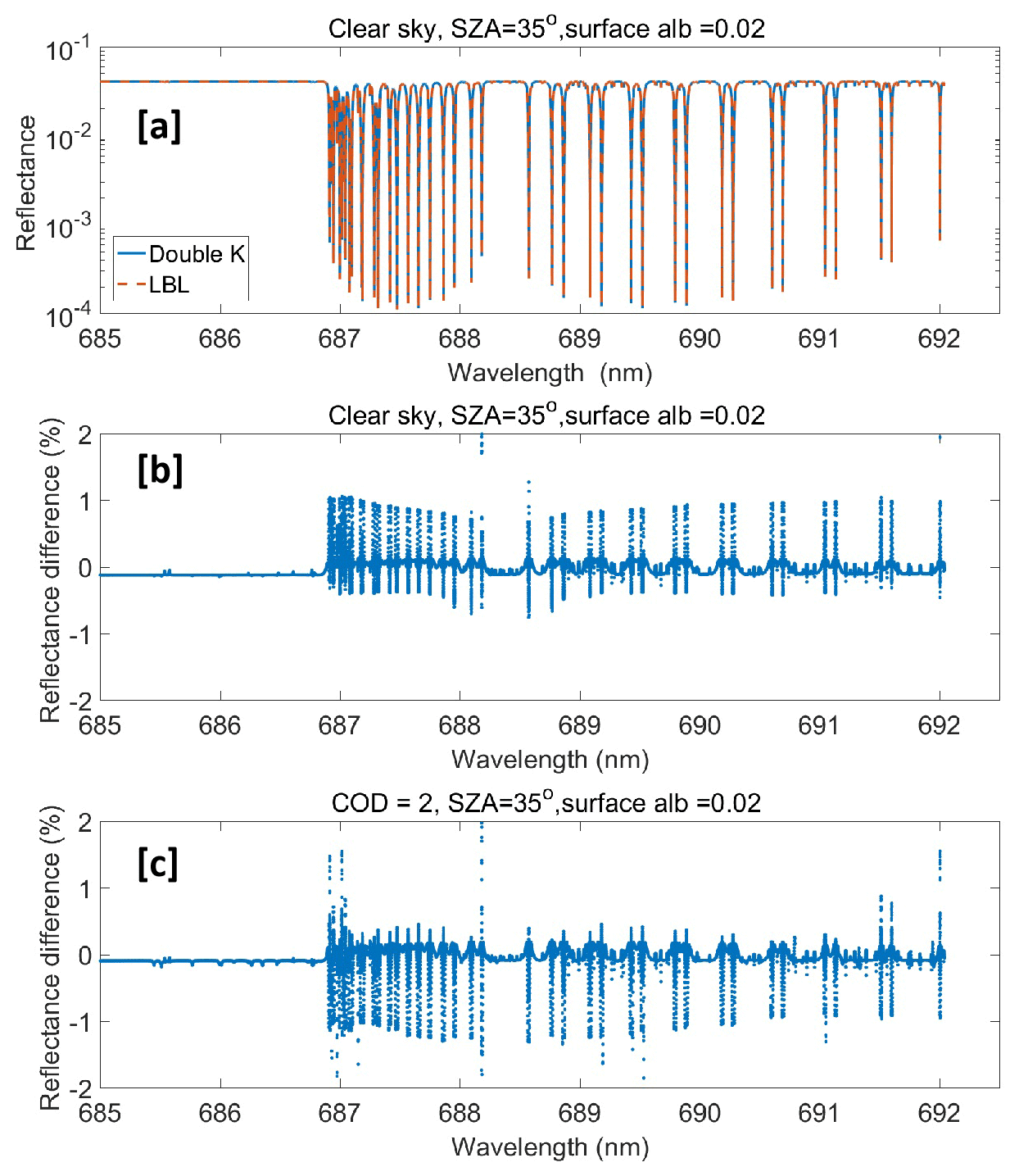
Figure 2 (a) High-resolution reflectance at the EPIC O₂ B band simulated by a fast radiative model (double-k) and benchmark (LBL). Difference between the simulated reflectance by (b) double-k and LBL for a clear-sky case and (c) a thin liquid water cloud case with COD 2. Here the SZA and view angle are 35^∘, the surface albedo is 0.02, the aerosol optical depth is 0.08, and the reflectance difference (%) is $\mathrm{100}\cdot \left(\right(\text{double}-k)-\text{LBL})/\text{LBL}$.

As shown in Fig. 2, under clear-sky and thin liquid water cloud situations, the simulated high-resolution upward diffuse oxygen B-band spectra from LBL calculation and the double-k approach are compared. The spectrum difference between LBL calculation and the double-k approach is very small (Fig. 2a). Under both situations, most of the relative difference between these two methods is under 0.5 %. The obvious relative difference (>1 %) occurs only in the wavelength range with high absorption optical depth, which has little contribution to the integrated solar radiation. Therefore, for the simulated narrowband measurements at the EPIC oxygen B band, the relative difference between LBL and the double-k approach is much smaller than that of the high-resolution spectrum, which is less than 0.1 % for a clear day. Compared to a clear-sky situation, the relative difference for cloud situations can be bigger. As shown in Table 1, the relative difference is −0.06 % and −0.32 % for typical high-level optical thin cloud and low-level thick cloud situations, respectively. The comparison of simulated narrowband measurements at the EPIC oxygen A-band channel (764 nm) is also shown in Table 1; the relative differences between LBL and the double-k approach are −0.06 %, 0.21 %, and 0.23 % for a clear day, high-level thin cloud, and low-level thick cloud cases, respectively. In general, the accuracy of double-k approach for both oxygen A and B absorption bands is high.

Table 1 Comparison of simulated narrowband measurement at EPIC A- and B-band channels.

2.3.3 Simulation of oxygen A and B bands for different atmospheric conditions

Using the EPIC measurement simulation package, we made a series of simulations with different settings for surface albedo, solar zenith angle, COD, CTH (CTP), and cloud geometric (pressure) thickness (or cloud-bottom height). The results of these simulations consist of a data table, which can be used not only to calculate the coefficients for the analytic equation, but also to study the sensitivity of every variable.

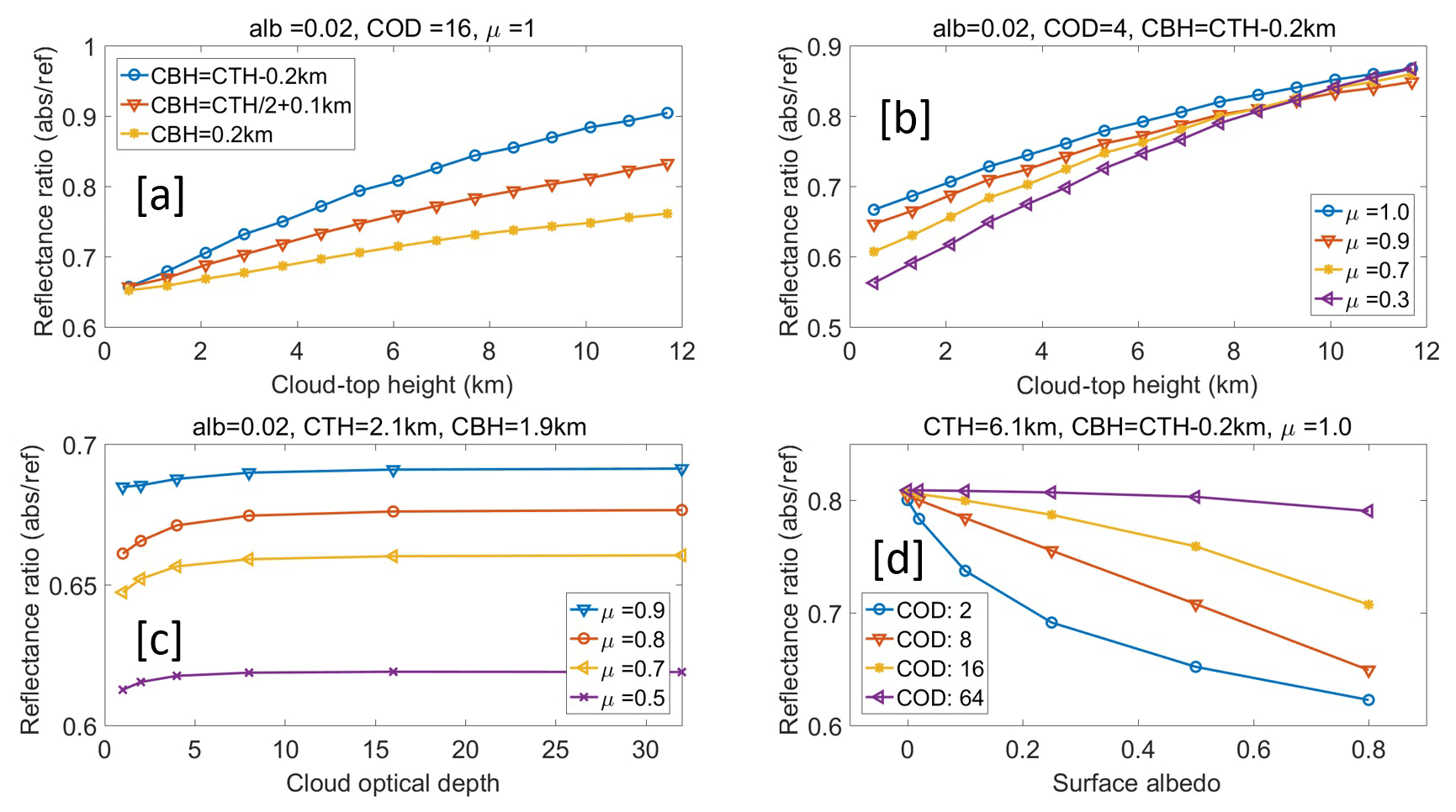
Figure 3 Ratio of simulated reflectance measurements for the EPIC B-band to B-band reference with different surface albedo (alb), COD, μ (cosine of solar zenith angle), cloud-top height (CTH), and cloud-bottom height (CBH).

According to the previous theory analysis, the ratio of reflectance radiance (i.e., absorption to the reference) at TOA is determined by the photon path length distribution at oxygen A and B bands: the larger the mean photon path length, the stronger the absorption and the smaller the reflectance ratio. To make the figures easy to view and understand, we use the cloud-top and cloud-bottom geometric height to represent CTP and thickness information in Fig. 3. As shown in Fig. 3a, the ratio of upward diffuse radiance at the oxygen B band and its reference band is sensitive to the cloud-top height (pressure). The higher the CTH, the larger the ratio. At the same time, this ratio is affected by the cloud-bottom height (or cloud geometric thickness) when the other cloud parameters are fixed; the lower the cloud bottom (or the larger the cloud geometric thickness), the smaller the ratio. It is consistent with the theory analysis: (1) the higher the CTH, the shorter the mean photon path length and the weaker the absorption. (2) When the COD is given, larger cloud geometric thickness means smaller cloud density, and sunlight can penetrate deeper into the cloud, which results in a longer mean photon path length. In Fig. 3b, for clouds with given CTH, COD, and geometric thickness, the ratio decreases with the solar and view angles. This can be understood to mean that the larger the solar and view angles, the longer the mean photon pathlength and the stronger the absorption. In Fig. 3c, for clouds with given CTH and geometric thickness, when the COD is small (e.g., COD <5), the reflectance ratio increases with COD. However, when COD is larger than 16, the effect of COD is small. This is because the larger the COD, the shallower the sunlight penetration, and the shorter the mean photon pathlength. In Fig. 3d, for clouds with given COD, CTP, and geometric thickness, the ratio decreases with surface albedo. The smaller the COD, the stronger the impact of the surface albedo. This is because thick cloud prevents incident sunlight from passing through it to reach the surface and also prevents reflected light from going back to the TOA.

For the oxygen A band, the ratio of upward diffuse radiance at absorption and reference bands shows similar characteristics as the oxygen B band. Compared to the oxygen B band, under the same atmospheric conditions, the oxygen absorption at the A band is stronger, and the ratio of the A band to its reference band has smaller values (shown in Fig. 4). As stated previously, for land area covered with plants, the surface albedo may change substantially from the oxygen B band to A band due to the presence of the red edge. Therefore, accurate spectral data on surface albedo for CTP retrieval are vitally important, especially for optically thin clouds.

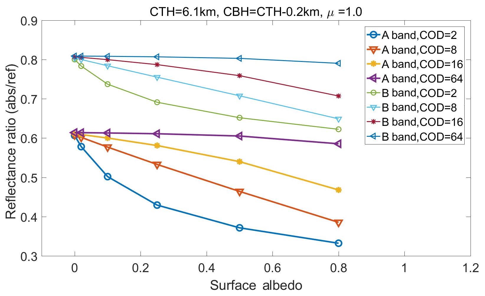
Figure 4 Ratio of simulated reflectance measurements for EPIC A and B absorption band to the reference band with different surface albedo.

3 Application and validation of the CTP retrieval method

3.1 Case studies of CTP retrieval

The dataset of DSCOVR EPIC measurements at 00:17:51 GMT on 25 July 2016 is used for the case studies. The reflectance at oxygen A and B bands with related solar zenith and viewing angles is obtained from the EPIC Level 1B data; COD information (retrieved from other EPIC channels) is obtained from EPIC Level 2 data. The surface albedo data are obtained from Global Ozone Monitoring Experiment 2 (GOME-2) surface Lambertian-equivalent reflectivity (LER) data. Detailed information on the datasets is shown in the “Data availability” section. To reduce the impact of the Earth's surface, we selected the region located in the spatial range of 75^∘ S to 85^∘ N and 177 to 175^∘ W for case studies, which is mainly covered by ocean. To constrain the influence of surface albedo and broken clouds, only pixels with total cloud cover (i.e., EPIC cloud mask 4), surface albedo less than 0.05, and liquid assumed COD larger than 3 are considered. In the selected region, around 10 000 pixels are finally chosen for case studies.

In our retrieval algorithm, we have two kinds of retrieval results: baseline CTP and retrieved CTP. The baseline CTP is used as a reference for the retrieved CTP. It is similar to the effective CTP in Yang et al. (2019), which does not consider cloud penetration. The retrieved CTP is calculated by the analytic equation, which considers in-cloud and below-cloud interactions.

During the baseline CTP calculation, the impact of in-cloud penetration is ignored, and the incident light that reached cloud top is assumed to be reflected back directly. As shown in Eq. (19), the baseline absorption optical depth τ_base is derived from the ratio of upward diffuse radiance at absorption bands and their reference bands directly. According to the model-calculated oxygen A- and B-band absorption optical depth profile at the specific solar zenith angle, the baseline CTP can be derived directly.

$$\begin{array}{}\text{(19)}& {\mathit{\tau }}_{\mathrm{base}}=\log \left(-{\displaystyle \frac{R_{\mathrm{abs}}}{R_{\mathrm{ref}}}}\right)/\left({\displaystyle \frac{\mathrm{1}}{\cos \left({\mathit{\theta }}_{\mathrm{sza}}\right)}}+{\displaystyle \frac{\mathrm{1}}{\cos \left({\mathit{\theta }}_{\mathrm{view}}\right)}}\right)\end{array}$$

As shown in Fig. 5, the baseline CTP value at the A band is slightly higher than the effective CTP from NASA ASDC L2 data. But the baseline CTP value at the B band is substantially higher than the effective CTP from NASA ASDC L2 data. For both the A band and B band, the difference between baseline CTP and effective CTP increases with the CTP. For low-level clouds, the mean differences are up to 60 and 100 mb at the A band and B band, respectively. The difference may be mainly from the calculation of oxygen A- and B-band absorption coefficients or the absorption optical depth profile.

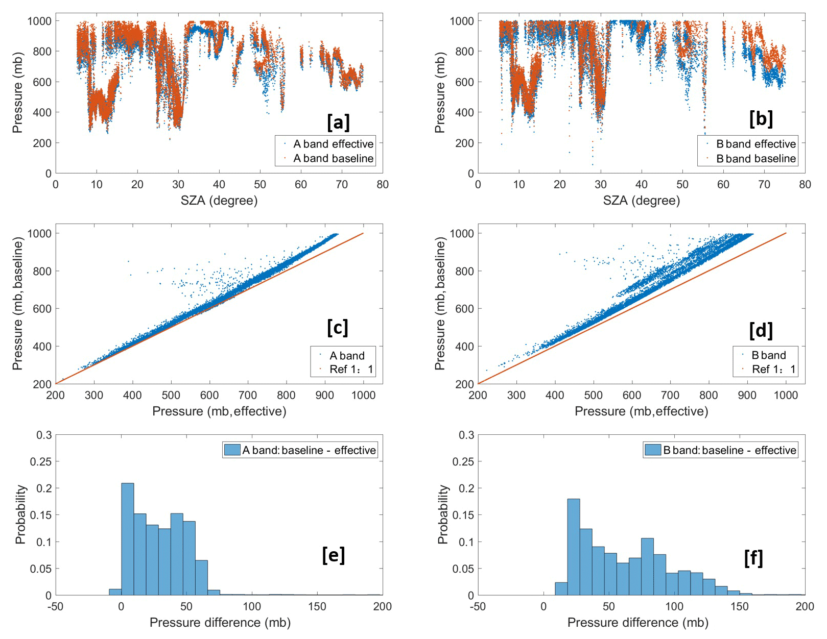
Figure 5 The comparison of effective CTPs (reference from NASA ASDC data) and baseline CTPs from our retrieval algorithm for the EPIC A and B bands.

Based on the simulated reflectance ratio under different atmospheric conditions, we can calculate the coefficients for the analytic radiative transfer equations by using a nonlinear fitting algorithm. The coefficients for different SZAs are calculated individually to reduce the fitting error. Based on the calculated coefficients, we can retrieve the CTP with DSCOVR EPIC observation data at the oxygen A and B bands.

During the CTP retrieval, with the exception of the previously mentioned analytic equation coefficients, we can get the surface albedo data from GOME and obtain reflectance data, solar zenith angle, view angles, and COD from the NASA ASDC data file. Another very important step in the retrieval processing is the acquisition of cloud pressure thickness data, which have a substantial impact on the retrieval results. We currently use a statistical approach (i.e., cloud pressure thickness (mb) $=\mathrm{2.5}\times \text{COD}+\mathrm{23}$) to estimate the cloud pressure thickness based on COD. As shown in Fig. 6a–d, the retrieved CTP when considering cloud penetration is smaller than baseline CTP. For this case, the mean differences between baseline CTP and retrieved CTP for the oxygen A band and B band are around 57 and 85 mb, respectively, which is consistent with theoretical expectations. For clouds with a given CTP, the mean photon path length will increase substantially when considering cloud penetration. A decrease in retrieved CTP will result in order to match the measurement ratio of absorption to reference. Compared to the O₂ A band, both baseline CTP and retrieved CTP for the O₂ B band are larger (Fig. 6e–h). This is because the absorption of solar radiation in the O₂ B band is weaker than that of the O₂ A band, and the incident light at the oxygen B band can penetrate deeper into the cloud, allowing more light to pass through. The difference in retrieved CTP between the B band and A band (approx. 93 mb with a standard deviation of 83 mb) is generally reduced in comparison to baseline B band and A band (approx. 114 mb with a standard deviation of 73 mb). This indicates, as expected, more photon penetration correction for the B band than the A band.

Figure 6 (a–d) The comparison of retrieved CTPs and baseline CTPs for EPIC A and B bands; (e, f) the comparison of retrieved CTPs and baseline CTPs between EPIC A and B bands.

We also used the LUT-based method to perform the retrieval for the same observation data because both methods share the same EPIC simulation package and the same simulated data table, the results of which are similar.

3.2 Validation of the retrieval method

To validate the analytic transfer inverse model method for CTP retrieval, we used another independent measurement of CTP, i.e., cloud layer top pressure from Cloud–Aerosol Lidar and Infrared Pathfinder Satellite Observations (CALIPSO; Vaughan et al., 2004), as a reference. For the previously stated case, i.e., DSCOVR EPIC measurements at 00:17:51 GMT on 25 July 2016, we used the cloud layer data from the CALIPSO IIR version 4.2 Level 2 product with 5 km resolution at 00:01:47 GMT on 25 July 2016 as its reference for validation. To constrain the error from spatial differences between different satellite measurements, we only chose the pixels of EPIC and CALIPSO measurements with a spatial distance of within 0.1^∘ (degree of latitude or longitude) to make comparisons. For the EPIC measurements, the same as previously stated, only pixels with total cloud cover (i.e., EPIC cloud mask 4), surface albedo less than 0.05, and liquid assumed COD larger than 3 are considered. As shown in Fig. 7a, there is a series of pixels (around 400 cases) from EPIC and CALIPSO measurements that can be used for the validation analysis. For reader convenience, we perform the analyses by using the case number as the x axis. Figure 7b shows the comparisons of cloud layer top pressure from CALIPSO and different CTPs (i.e., effective CTP, baseline CTP, and retrieved CTP) from EPIC measurements. Figure 7c shows the cloud layer number measured by CALIPSO. According to Fig. 7b and c, we can get some results: under single-layer cloud situations, the CTPs derived from EPIC measurements are close to the CTP from CALIPSO; under multilayer cloud situations, the CTPs derived from EPIC measurements are larger than the CTP from CALIPSO. Figure 7d shows the expanded view of Fig. 7b for some cases under single-layer cloud situations. For these single-layer cloud cases (with case numbers 46–156), the mean values of CTP for CALIPSO, EPIC effective, EPIC baseline, and EPIC retrieval are 846, 834, 866, and 850 mb, respectively. Compared to the CTP from CALIPSO measurements, the EPIC effective and baseline CTPs are 12 mb smaller and 20 mb larger, respectively; the EPIC retrieval with consideration of photon penetration is only 4 mb larger. This shows that our method for the CTP retrieval is valid and accurate under single-layer cloud situations with COD >3 and low surface albedo. Under multilevel cloud situations, high-level clouds are often thin clouds, which can be detected by CALIPSO but are hard to derive by our retrieval method. This is because the EPIC-retrieved CTP mainly shows the pressure of cloud layer that reflects the major part of incident sunlight.

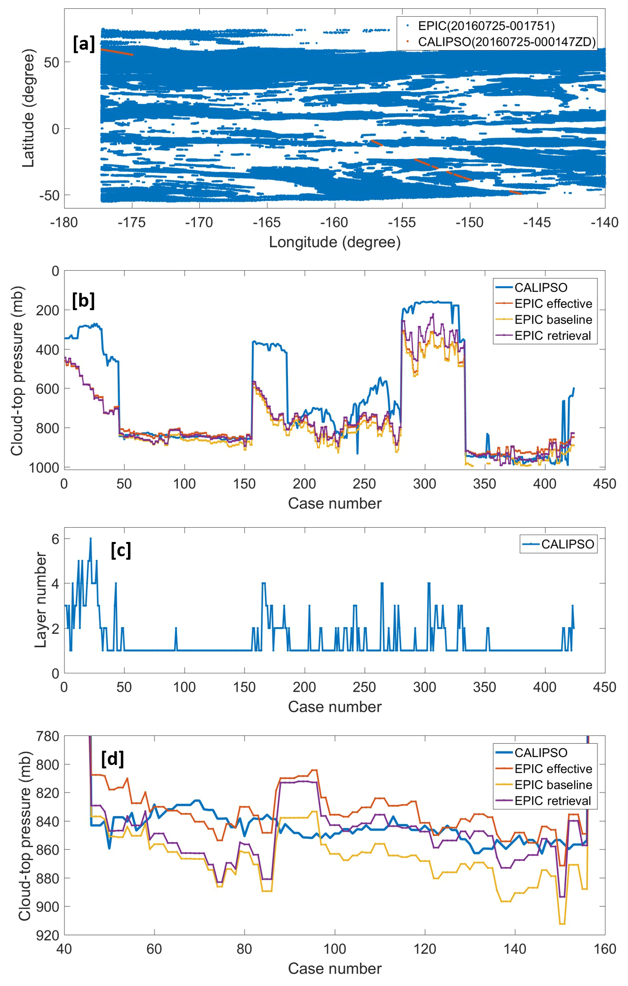
Figure 7 (a) The geolocation match of an EPIC measurement at 00:17:51 GMT and CALIPSO measurement at 00:01:47 GMT on 25 July 2016; (b) comparisons of cloud layer top pressure from CALIPSO measurements and the CTPs derived from EPIC measurements; (c) the cloud layer number from CALIPSO measurements; and (d) the expanded view of (b) for some cases under single-layer cloud situations.

3.3 Retrieval of global observation

We applied our retrieval algorithm to global DSCOVR EPIC measurement data at oxygen A and B bands. During the retrieval, only pixels with total cloud cover (i.e., cloud mask index of 4), surface albedo <0.25, and COD ≥3 are considered. To make the pictures easy to visualize and analyze, all invalid values are plotted as white (or blank) pixels.

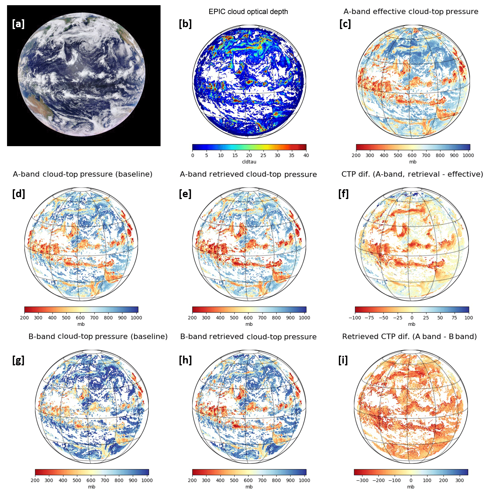
Figure 8 (a) RGB image from a DSCOVR EPIC measurement at 00:17:51 GMT on 25 July 2016; (b, c) COD (liquid assumption) and A-band effective CTP from NASA ASDC EPIC L2 products. (d, e) Baseline and retrieved CTP derived from EPIC A-band measurement; (f) the difference of the A-band retrieved CTP and A-band effective CTP. (g, h) Baseline and retrieved CTP derived from EPIC B-band measurement; (i) the difference of retrieved CTP between the EPIC A band and B band.

Figure 8a shows the synthesized RGB (red, green, blue) picture of EPIC measurements at 00:17:51 GMT on 25 July 2016. At this point in time sunlight covers most of the Pacific Ocean. In this figure, the white pixels represent cloud cover. Figure 8b shows the global COD (NASA ASDC L2 data), in which the white areas and colorful areas indicate clear-sky areas and cloudy areas, respectively. On the whole, the cloudy areas are consistent with the RGB image. The highlighted (red) areas indicate that the cloud systems there contain optically heavy clouds. Figure 8c shows the A-band effective CTP (NASA ASDC L2 data); the white areas indicate clear sky or no valid values, and warm (brown) and cold (blue) color areas indicate high-level and low-level clouds, respectively. According to the A-band effective CTP, high-level clouds are dominant in the equatorial area, and low-level clouds play a major role in the cloud systems in the North Pacific area. Figure 8d and e show the baseline and retrieved CTP at the A band, respectively, in which cloudy areas are consistent with the A-band effective CTP image on the whole. Due to the filtering setting in the CTP retrieval algorithm, there are more white pixels (invalid values) in these two figures. The difference in the A-band retrieved CTP and A-band effective CTP is shown in Fig. 8d. The A-band retrieved CTP is overall smaller than A-band effective CTP, with a difference within 100 mb. The highlighted (brown or red) areas are located in high-level cloud areas or large COD areas. This indicates that the complexity of a cloud system has a significant impact on the CTP retrieval. Figure 8g and h show the baseline and retrieved CTP in the B band, respectively, which are similar to but greater than the A band. As shown in Fig. 8i, the retrieved CTP at the EPIC B band is overall significantly larger than the retrieved CTP at the EPIC A band, for which the mean difference is up to 200 mb.

As previously stated in Sect. 3.2, under single-layer cloud situations, the CTPs derived from EPIC A-band measurements have good agreement with the CTP from CALIPSO measurements; under multiple-layer cloud situations, the CTPs derived from EPIC measurements may be larger than the CTPs of high-level thin clouds due to the effect of photon penetration. Therefore, in the global range for large-scale low-level stratus clouds, the retrieved CTPs from EPIC A-band measurements should agree well with the actual value of CTPs, but for a complex cloud system with multiple-layer clouds, the CTPs derived from EPIC A-band measurements may be larger than those of high-level thin clouds.

4 Conclusion

In-cloud photon penetration has significant impacts on the CTP retrieval when using DSCOVR EPIC oxygen A- and B-band measurements. To address this issue, we proposed two methods: (1) the LUT-based method and (2) the analytic transfer inverse model method for CTP retrieval with consideration of in-cloud photon penetration. In the analytic transfer inverse model method, we build an analytic equation that represents the reflection at TOA from above cloud, in cloud, and below cloud. The coefficients of this analytic equation can be derived from a series of EPIC simulations under different atmospheric conditions using a nonlinear regression algorithm. With EPIC observation data, the related solar zenith and sensor view angle, surface albedo data, COD, and estimated cloud pressure thickness, we can retrieve the CTP by solving the analytic equation.

We developed a package for the DSCOVR EPIC measurement simulation. The high-resolution radiation spectrum must be simulated first and then integrated with the EPIC filter function in order to accurately simulate EPIC measurements. Because this process is highly time-consuming, a polynomial fitting function is used when calculating the oxygen absorption coefficients under different atmospheric conditions. At the same time, the double-k approach is applied to the high-resolution spectrum simulation to further reduce time costs, which can obtain high-accuracy results with a 100-fold time reduction. The results of the EPIC simulation measurements are consistent with theoretical analysis.

Based on the EPIC simulation measurements, we derived a series of coefficients from various solar zenith angles for the analytic EPIC equations. Using these coefficients, we performed CTP retrieval for real EPIC observation data. We have two kinds of retrieval results: baseline CTP and retrieved CTP. The baseline CTP is similar to the effective CTP in Yang et al. (2019), which does not consider cloud penetration. The retrieved CTP is derived by solving the analytic equation with the consideration of in-cloud and below-cloud interactions. Compared to the effective CTP provided by NASA ASDC L2 data, the baseline CTP value at the A band is slightly higher, but the baseline CTP value at the B band is substantially higher. The retrieved CTP for both the oxygen A and B bands is smaller than the related baseline CTP. At the same time, compared to the oxygen A band, both baseline CTP and retrieved CTP at the oxygen B band are larger. The cloud layer top pressure from CALIPSO measurements is used to validate the CTP derived from EPIC measurements. Under single-layer cloud situations, the retrieved CTPs for the oxygen A band agree well with the CTPs from CALIPSO, for which the mean difference is within 5 mb in the case study. Under multiple-layer cloud situations, the CTPs derived from EPIC measurements may be larger than the CTPs of high-level thin clouds due to the effect of photon penetration.

Currently, this analytical transfer model method can only retrieve CTP, and it still requires cloud pressure thickness as an input parameter. However, in the satellite observations, both CTP and cloud pressure thickness are unknown. The estimation or assumption of cloud pressure thickness will bring extra error into CTP retrieval. In the near future, we plan to address this issue.