the Creative Commons Attribution 4.0 License.
the Creative Commons Attribution 4.0 License.
 | 14 Oct 2020
Leveraging spatial textures, through machine learning, to identify aerosols and distinct cloud types from multispectral observations
Willem J. Marais
Robert E. Holz
Jeffrey S. Reid
Rebecca M. Willett
Current cloud and aerosol identification methods for multispectral radiometers, such as the Moderate Resolution Imaging Spectroradiometer (MODIS) and Visible Infrared Imaging Radiometer Suite (VIIRS), employ multichannel spectral tests on individual pixels (i.e., fields of view). The use of the spatial information in cloud and aerosol algorithms has been primarily through statistical parameters such as nonuniformity tests of surrounding pixels with cloud classification provided by the multispectral microphysical retrievals such as phase and cloud top height. With these methodologies there is uncertainty in identifying optically thick aerosols, since aerosols and clouds have similar spectral properties in coarse-spectral-resolution measurements. Furthermore, identifying clouds regimes (e.g., stratiform, cumuliform) from just spectral measurements is difficult, since low-altitude cloud regimes have similar spectral properties. Recent advances in computer vision using deep neural networks provide a new opportunity to better leverage the coherent spatial information in multispectral imagery. Using a combination of machine learning techniques combined with a new methodology to create the necessary training data, we demonstrate improvements in the discrimination between cloud and severe aerosols and an expanded capability to classify cloud types. The labeled training dataset was created from an adapted NASA Worldview platform that provides an efficient user interface to assemble a human-labeled database of cloud and aerosol types. The convolutional neural network (CNN) labeling accuracy of aerosols and cloud types was quantified using independent Cloud-Aerosol Lidar with Orthogonal Polarization (CALIOP) and MODIS cloud and aerosol products. By harnessing CNNs with a unique labeled dataset, we demonstrate the improvement of the identification of aerosols and distinct cloud types from MODIS and VIIRS images compared to a per-pixel spectral and standard deviation thresholding method. The paper concludes with case studies that compare the CNN methodology results with the MODIS cloud and aerosol products.
- Article
(14558 KB) - Full-text XML
- BibTeX
- EndNote


A benefit of polar-orbiting satellite passive radiometer instruments, such as the Moderate Resolution Imaging Spectroradiometer (MODIS); Visible Infrared Imaging Radiometer Suite (VIIRS); and constellation of geostationary sensors, such as with the Advance Baseline Imager (ABI) and Advanced Himawari Imager (AHI), is their ability to resolve the spatial and spectral properties of clouds and aerosol features while providing global coverage. Consequently, the optical property measurements of aerosol particles and clouds from radiometer instruments dominate both the atmospheric research and operational communities (Schueler et al., 2002; Salomonson et al., 1989; Klaes et al., 2013; Parkinson, 2013; Platnick et al., 2016; Levy et al., 2013; Al-Saadi et al., 2005). For example, cloud and aerosol measurements on a global scale are routinely employed in advance modeling systems such as those contributing to the International Cooperative for Aerosol Prediction multi‐model ensemble (ICAP-MME; Xian et al., 2018) and the NASA Goddard Earth Observing System version 5 (GEOS-5) models (Molod et al., 2012).
Our work in this paper is motivated by two related atmospheric research needs:
-
Current data assimilation and climate applications depend on the accurate identification of optically thick aerosols from radiometer images on global scales; Figs. 1 and 2 illustrate the difficulty in identifying optically thick aerosols and cloud types, which is due to the low spectral contrast between optically thick aerosols and water clouds in individual fields of view (FOVs).
-
Climatological research can benefit from the identification of major cloud regimes, as illustrated in Fig. 2, since meteorological conditions and major cloud regimes are related due to the strong correlations between cloud types and atmospheric dynamics (Levy et al., 2013; Tselioudis et al., 2013; Evan et al., 2006; Jakob et al., 2005; Holz, 2002); very little work has been done on cloud-type identification from radiometer images.
What both these research needs have in common is that a practitioner uses contextual differences, such as spatial and spectral properties (e.g., patterns and “color”), to identify optically thick aerosols and cloud types from imagery. For example, from Figs. 1 and 2, a practitioner would use spatial texture to make distinctions between optically thick aerosols and closed-stratiform and cirrus clouds. Although practitioners can visually make these distinctions, current operational NASA cloud and aerosol products are not able to reliably identify optically thick aerosols and cloud types. Specifically, illustrated by Figs. 1 and 2, (1) NASA cloud products mistake optically thick aerosols for clouds, (2) the aerosol optical depth (AOD) retrieved by the NASA aerosol products of optically thick aerosols are labeled as “bad” by the quality control flags, and (3) from the NASA cloud optical properties product it is unclear how to distinguish different cloud types other than making a distinction between water and ice clouds. Consequently, in a climatological research project involving aerosols, most large-impact optically thick aerosols will be excluded in the research study if the project relies on the MODIS level-2 cloud and aerosol products; this problem stresses the importance of the reliable identification of optically thick aerosols.
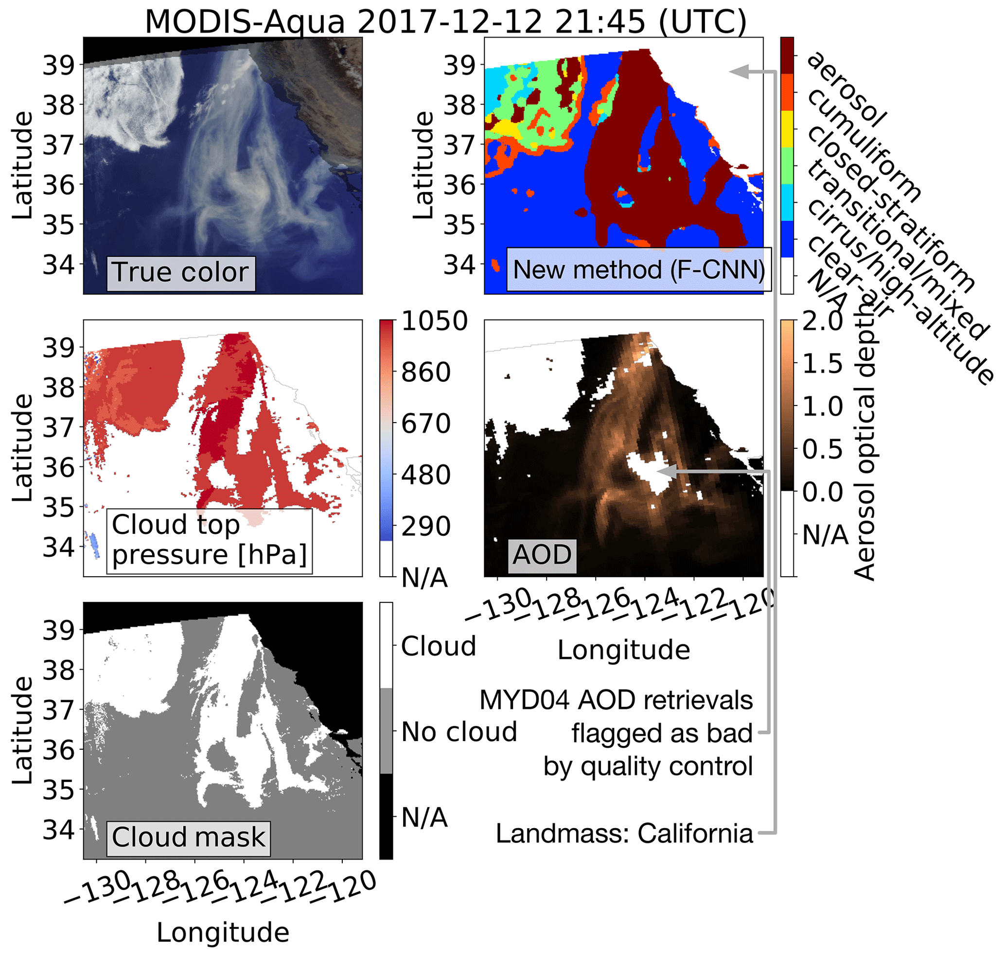
Figure 1These images show an example where the MODIS spectral and standard deviation thresholding (SSDT) techniques misclassify a thick smoke plume as a cloud; the smoke plume originated from Oregon, and measurements were taken on 12 December 2017 with MODIS-Aqua. According to the MODIS cloud top pressure (MYD06) and mask (MYD35) products, the whole smoke plume is labeled as a cloud. The MYD04 aerosol product associates the optically thick part of the smoke plume with “bad” quality control flags, since the SSDT technique employed by the MYD04 product is tuned to aggressively ignore any observations that have a close resemblance to a cloud. The new methodology uses a convolutional neural network to extract spatial texture features which enables the method to make an accurate distinction between aerosols that have smooth surfaces and clouds that have nonsmooth surfaces.

Figure 2These images show the different texture smoothness properties of the stratiform, cumuliform and cirrus/high-altitude cloud at different spectral channels and how the proposed methodology (i.e., the new method) was able to leverage the smoothness properties to make a distinction between different cloud types. Stratiform clouds are smoother than cumuliform clouds, and both stratiform and cumuliform clouds are smoother than cirrus/high-altitude clouds at 11 µm brightness temperature. From the MYD06 cloud-phase product it is unclear how to set different cloud types apart other than cirrus/high-altitude clouds.
The underutilization of spatial information in radiometer images is a major reason why NASA operational cloud and aerosol products struggle to identify optically thick aerosols and restrain the identification of different cloud types; most NASA products operate on primarily spectral information of individual pixels and some simple spatial analysis such as standard deviation of image patches. This paper demonstrates that convolutional neural networks (CNNs) can increase the accuracy in identifying optically thick aerosols and provide the ability to identify different cloud types (Simonyan and Zisserman, 2014; LeCun et al., 1989; Krizhevsky et al., 2012; Szegedy et al., 2017; LeCun et al., 1998; LeCun, 1989).
Recent applications of statistical and machine learning (ML) methods in atmospheric remote sensing have demonstrated improvements upon current methodologies in atmospheric science. For example, neural networks have been employed to (1) approximate computationally demanding radiative transfer models to decrease computation time (Boukabara et al., 2019; Blackwell, 2005; Takenaka et al., 2011), (2) infer tropical cyclone intensity from microwave imagery (Wimmers et al., 2019), (3) infer cloud vertical structures and cirrus or high-altitude cloud optical depths from MODIS imagery (Leinonen et al., 2019; Minnis et al., 2016), and (4) predict the formation of large hailstones from land-based radar imagery (Gagne et al., 2019). Specific to cloud and volcanic ash detection from radiometer images, Bayesian inference has been employed where the posterior distribution functions were empirically generated using hand-labeled (Pavolonis et al., 2015) or coincident Cloud-Aerosol Lidar with Orthogonal Polarization (CALIOP) observations (Heidinger et al., 2016, 2012) or from a scientific product (Merchant et al., 2005).
Inspired by the recent successful applications of ML in atmospheric remote sensing, we hypothesize that a methodology can be developed that accurately identifies optically thick aerosols and cloud types by better utilizing the coherent spatial information in moderate-resolution multispectral imagery via recent advances in CNN architectures. Leveraging these recent advances we explore the following questions:
-
Can the application of CNNs with training data developed from a human-classified dataset improve the distinction between cloud and optically thick aerosol events and provide additional characterization of clouds, leveraging the contextual information to retrieve cloud type?
-
When identifying aerosols and cloud types by dividing up an image into smaller patches and extracting spatial information from the patches, what is the optimal patch size (number of pixels) that provides the best identification accuracy of the aerosols and cloud types?
-
How does the performance of the aerosol and cloud-type identification compare to lidar observations such as those of CALIOP?
We specifically consider a human-labeled dataset instead of using an active instrument such as CALIOP and the Cloud Profiling Radar (CPR) to produce a labeled dataset, since the cloud and aerosol products of these instruments have limitations; for example, the CPR only accurate detects precipitating clouds, and both CALIOP and the CPR are nadir-viewing instruments with which only a fraction of MODIS–VIIRS pixels can be labeled (Kim et al., 2013; Stephens et al., 2002).
To address the proposed questions above we developed a methodology in which we adopted a CNN to exploit both the spatial and spectral information provided by MODIS–VIIRS observations to make a distinction between basic categories of aerosol and cloud fields: clear-air, optically thick aerosol features, cumuliform cloud, transitional cloud, closed-stratiform cloud and cirrus/high-altitude cloud. To conceptually demonstrate the new capabilities, Figs. 1 and 2 show the results of the methodology which has identified (1) an optically thick aloft smoke plume and (2) cloud classification based on the contextual information. The capability to globally detect and monitor these cloud and aerosol types provides important new information about the atmosphere since these cloud types are strongly correlated with atmospheric dynamics (Tselioudis et al., 2013). This paper does not address identifying clouds by their specific forcing or physics; this is a topic of a subsequent paper; here, we are only interested in differentiating spatial cloud patterns and major aerosol events.
The work that we present in this paper has been primarily developed for daytime deep-ocean observations, since the identification of aerosols and cloud types over land and during the nighttime is a separate and challenging research project.
The outline of the paper is as follows. In Sect. 2 we describe the proposed methodology to identify aerosols and cloud types via a CNN; technical details of the methodology are in Appendices A and B. Included in Sect. 2 we (1) discuss why CNNs are capable of extracting spatial texture features from images, (2) explain why we use a pretrained CNN rather than training a CNN from radiometer images and (3) explain why the pretrained CNN extracts useful spatial texture features from radiometer images. In Sect. 3 we share test results of the proposed methodology using case studies. The paper is concluded in Sect. 4 with a discussion of future work. Appendix C gives an overview of the satellite instruments that are used in this paper.
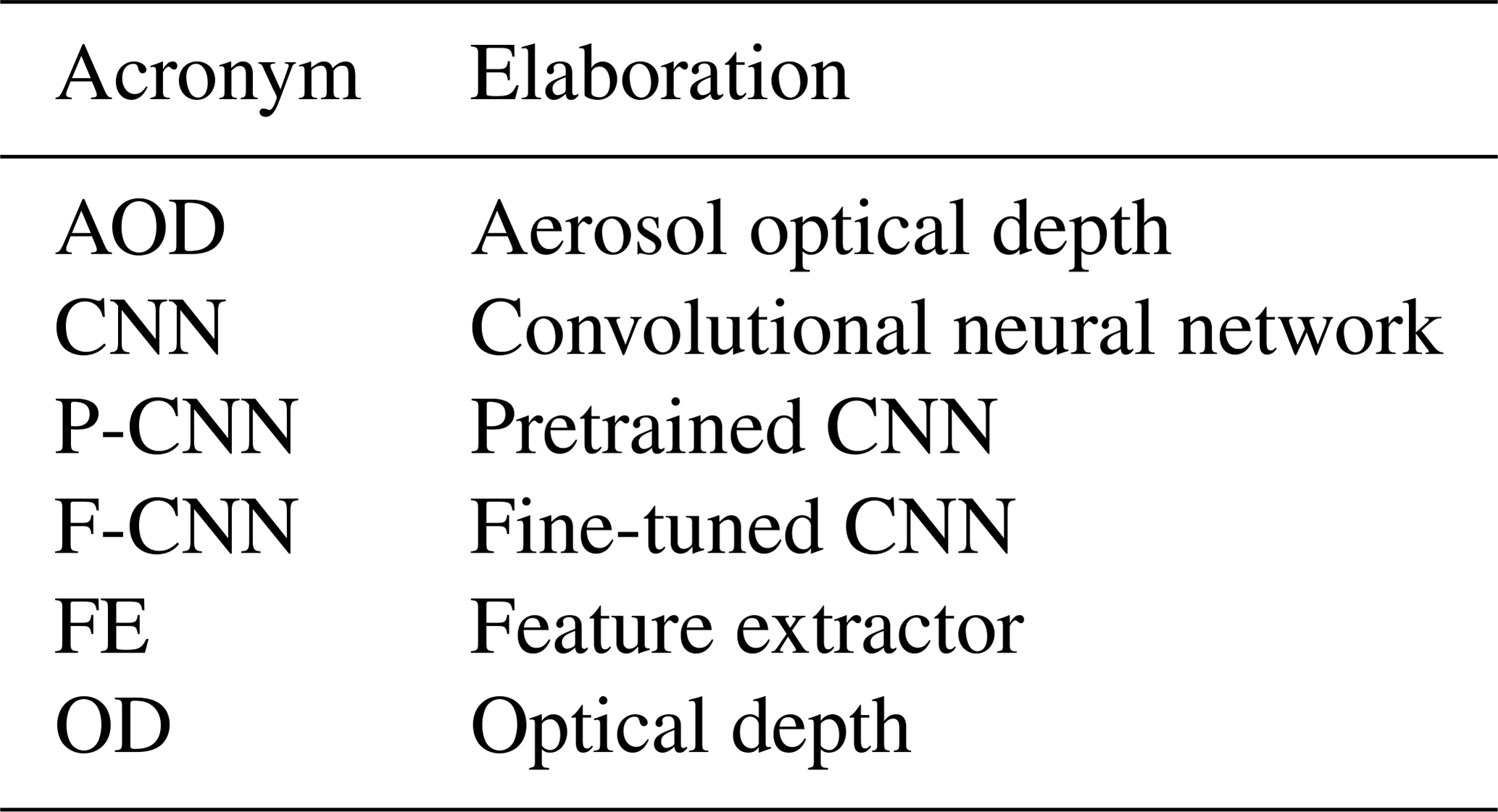
Table 1 shows commonly used acronyms that are used throughout this paper which the reader can reference for the sake of convenience.
Table 1Commonly used acronyms that are used throughout this paper.
The advantage of the proposed methodology is that it provides an approach to leveraging the contextual spatial information in radiometry imagery to (1) identify cloud types and (2) separate clouds from optically thick aerosol features. In comparison the MODIS–VIIRS cloud and aerosol algorithms employ per-pixel spectral and standard deviation (SD) thresholding techniques which correctly identify clouds overall; the simple spatial statistics, however, of the MODIS–VIIRS algorithms on different spectral images do not provide enough independent information to uniquely separate optically thick aerosol events from cloud (Platnick et al., 2016; Levy et al., 2013).
A small subset of a MODIS or VIIRS image, which we call a patch, is labeled as clear-air, optically thick aerosol, low-level to midlevel cumuliform cloud, transitional/mixed cloud (transitional between the two or mixed types), closed-stratiform cloud or cirrus/high-altitude cloud by the following two steps:
-
The contextual spatial and spectral information are extracted via a feature extractor (FE) algorithm.
-
With a multinomial classifier (i.e., multiclass classifier), which takes as input the extracted features, the patch is assigned probability values of being a specific cloud type or aerosol.
The cloud type or aerosol with the largest probability is the label assigned to the patch.
In this paper we define a method as a feature extractor (FE) algorithm with a multinomial classifier (Krishnapuram et al., 2005); our method employs a CNN as an FE algorithm, which simultaneously extracts spatial information from the 0.642 and 0.555 µm solar reflectances and the 11 µm brightness temperature (BT) measurements where each of the bands jointly provide key information to identify aerosols and distinct cloud types. The multinomial classifier has tuning parameters that are used when assigning probability values to extracted features of different cloud types and aerosols (Krishnapuram et al., 2005); these tuning parameters are estimated using a training dataset. Hence, a focus of the proposed methodology is the creation of a training dataset that enables a CNN to extract spatial features of aerosols and cloud types. We adapted the NASA Worldview web framework that enables an atmospheric scientist to hand-label aerosols and cloud types (NASA, 2020); Fig. 4 shows an example of the adapted user interface.
Cloud types and aerosols in a whole MODIS or VIIRS image are identified by (1) dividing the image into patches and (2) the method (FE and classifier) being applied to each patch to produce a label of clear-air, optically thick aerosol, low-level to midlevel cumuliform cloud, transitional/mixed cloud (transitional between the two or mixed types), closed-stratiform cloud or cirrus/high-altitude cloud. The size of the patches, from which the spatial features are extracted, determines the labeling image resolution; we show in the results how labeling accuracy is a function of the patch size. In this paper we consider patch sizes of 25 and 100 pixels where 1 pixel equals approximately 1 km.
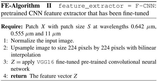
Since it is not clear which FE algorithm will yield spatial textual features that optimize the classification performance for identifying cloud types and aerosols, we consider three different FE algorithms: (1) pretrained CNN, (2) fine-tuned CNN and (3) traditional mean–standard deviation (MeanStd) FE algorithm as a control. We employ a pretrained CNN since a CNN requires a large training dataset (e.g., a million images) to estimate its parameters (Simonyan and Zisserman, 2014), whereas the pretrained CNN has its parameters pre-estimated from a different image classification problem (e.g., general internet images). A fine-tuned CNN has its parameters estimated from radiometer images where the initial values of the CNN parameters are from a pretrained CNN. The main purpose of the MeanStd FE is to set a baseline result.
The next subsection introduces the algorithms that estimate the parameters of the methods and apply the methods to radiometer images. In Sect. 2.2 we discuss how the labeled dataset, which is subdivided into a training and test dataset, is created; from the test dataset a test (generalization) error is computed with which we rank the different methods (Friedman et al., 2001). Section 2.3 gives a short overview of CNNs and elaborates on the pretrained and fine-tuned CNNs. Appendix B provide details of the pretrained CNN, fine-tuned CNN and MeanStd FE algorithms.
2.1 Algorithms that train and apply methods
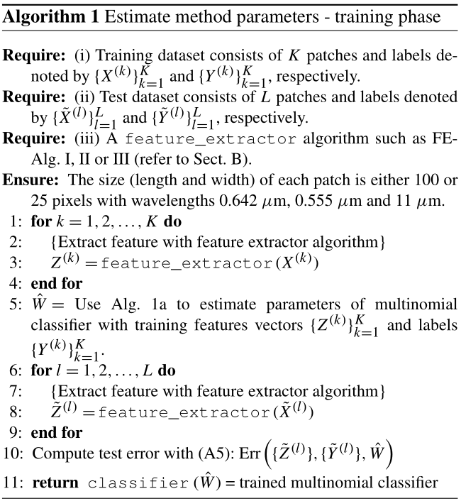
Two algorithms are used to (1) estimate the multinomial classifier parameters (i.e., training phase) of each method (i.e., multinomial classifier with an FE algorithm) and (2) apply each method to a MODIS or VIIRS image to label the pixels in the image as aerosol and cloud type. The first algorithm estimates a method's parameters from the labeled training datasets of patches, and the test error is computed from the labeled test datasets of patches; Fig. 3a gives a pictorial overview and Algorithm 1 in Appendix A1 gives a detailed outline of the first algorithm. The second algorithm applies a method (trained via Algorithm 1) on a MODIS or VIIRS image by dividing the input image into patches and applying the method on each patch; Fig. 3b gives a pictorial overview and Algorithm 2 in Appendix A2 gives a detailed outline of the second algorithm.
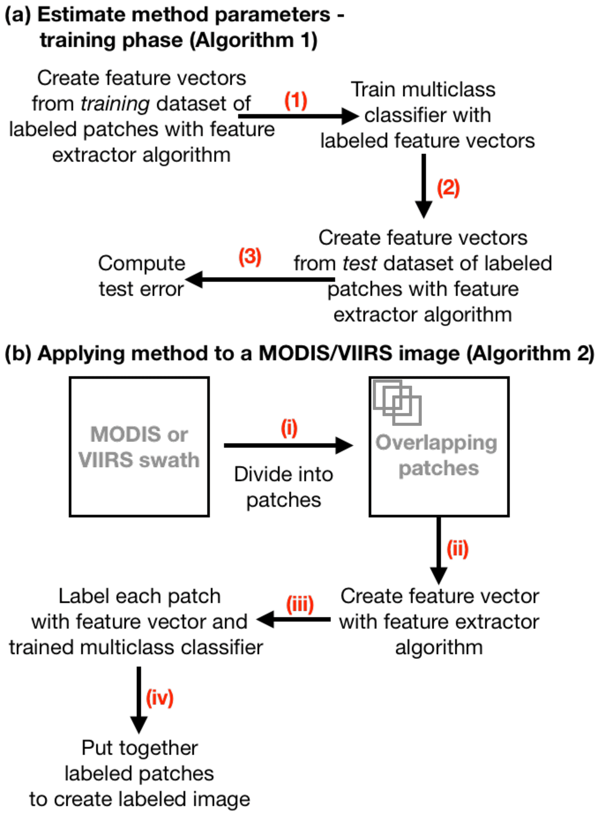
Figure 3A method that identifies cloud types and aerosols in MODIS–VIIRS images consists of a feature extractor (FE) algorithm and a multiclass classifier. (a) The parameters of the method's multiclass classifier are estimated and the test error is computed by (1) creating the feature vectors from each patch in the training dataset via the method's FE algorithm, (2) estimating the multiclass classifier's parameters using the training feature vectors and the corresponding labels, and (3) extracting the feature vectors from each patch in the test dataset and computing the test error from the test feature vectors and corresponding labels. (b) A trained method is applied to a MODIS or VIIRS image by (i) dividing the MODIS or VIIRS image into overlapping patches, (ii) extracting for each patch the spatial texture feature vectors via the method's FE algorithm, (iii) labeling each patch via the feature vector and the method's trained multiclass classifier, and (iv) putting together all the labeled patches to create a labeled image.
2.1.1 Algorithm 1 – estimate method parameters – training phase
Algorithm 1 takes as input the labeled training and test datasets of patches with the given FE algorithm, and the output is a trained multinomial classifier and test error (Krishnapuram et al., 2005; Friedman et al., 2001). For each patch the multinomial classifier models a probability value for each label. This probability model has several parameters that are estimated from the labeled training dataset by finding the parameters that minimizes an objective (i.e., cost) function; the objective function consists of (1) a loss function that fits the parameters onto the patches and labels and (2) a l2 (Euclidean norm) penalty function with a tuning parameter that regularizes the parameters to prevent the multinomial classifier from overfitting on the training dataset (Friedman et al., 2001). The optimum tuning parameter is estimated via 5-fold cross validation, since the size of our training dataset is limited (Friedman et al., 2001). Once the multinomial classifier has been trained the test dataset is used to compute a test error for the method by labeling the patches in the test dataset and computing the labeling accuracy.
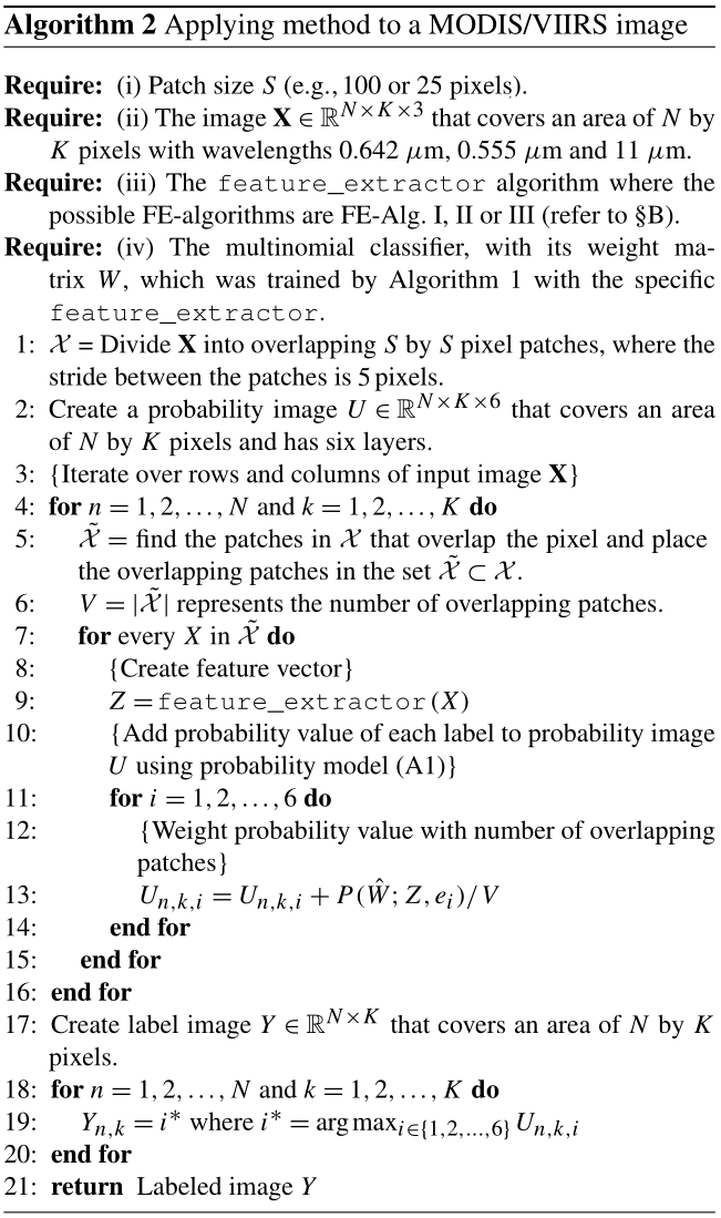
2.1.2 Algorithm 2 – applying trained method to label a MODIS or VIIRS image
Algorithm 2 takes as input a MODIS or VIIRS image, patch size and a trained method which consists of an FE algorithm with its corresponding trained multinomial classifier. For every pixel in the input MODIS or VIIRS image, Algorithm 2 assigns a label to the pixel by (1) computing what is the probability that pixel belongs to one of the six label categories (clear-air, optically thick aerosol, etc.) and (2) assigning the label with maximum probability value to the corresponding pixel. To assign a probability value of a specific label to a pixel, Algorithm 2 in summary (1) takes all the patches that intersects with the target pixel, (2) extracts the feature vectors from the patches with the given FE algorithm, (3) applies the multinomial classifier on each feature vector to produce a series of probability values (of the specific label) and (4) averages the series of probability values to produce a final probability value of the target pixel. This labeling procedure assumes that the category to which a pixel belongs is correlated with the categories of the surrounding pixels, implying that all patches that intersect a pixel contribute to the probability value of the pixel.
In order to reduce the computational demand on estimating the probability values per pixel, the overlapping patches have a row and column index stride of 5.
2.2 The labeled dataset
The labeled dataset, from which each method's parameters and error performance are estimated, is created through an adapted Space Science Engineering Center (SSEC) NASA Worldview web interface; the website allows an atmospheric scientist to interactively create a labeled dataset. Figure 4 shows how the labeled dataset is assembled; the subset MODIS–VIIRS images that are chosen are divided into overlapping patches of the two different sizes of 25 and 100 pixels. From the labeled dataset a training and a test dataset are created by sampling from labeled datasets; the training and test datasets are used to estimate the parameters and error performance of a method, respectively (Friedman et al., 2001).
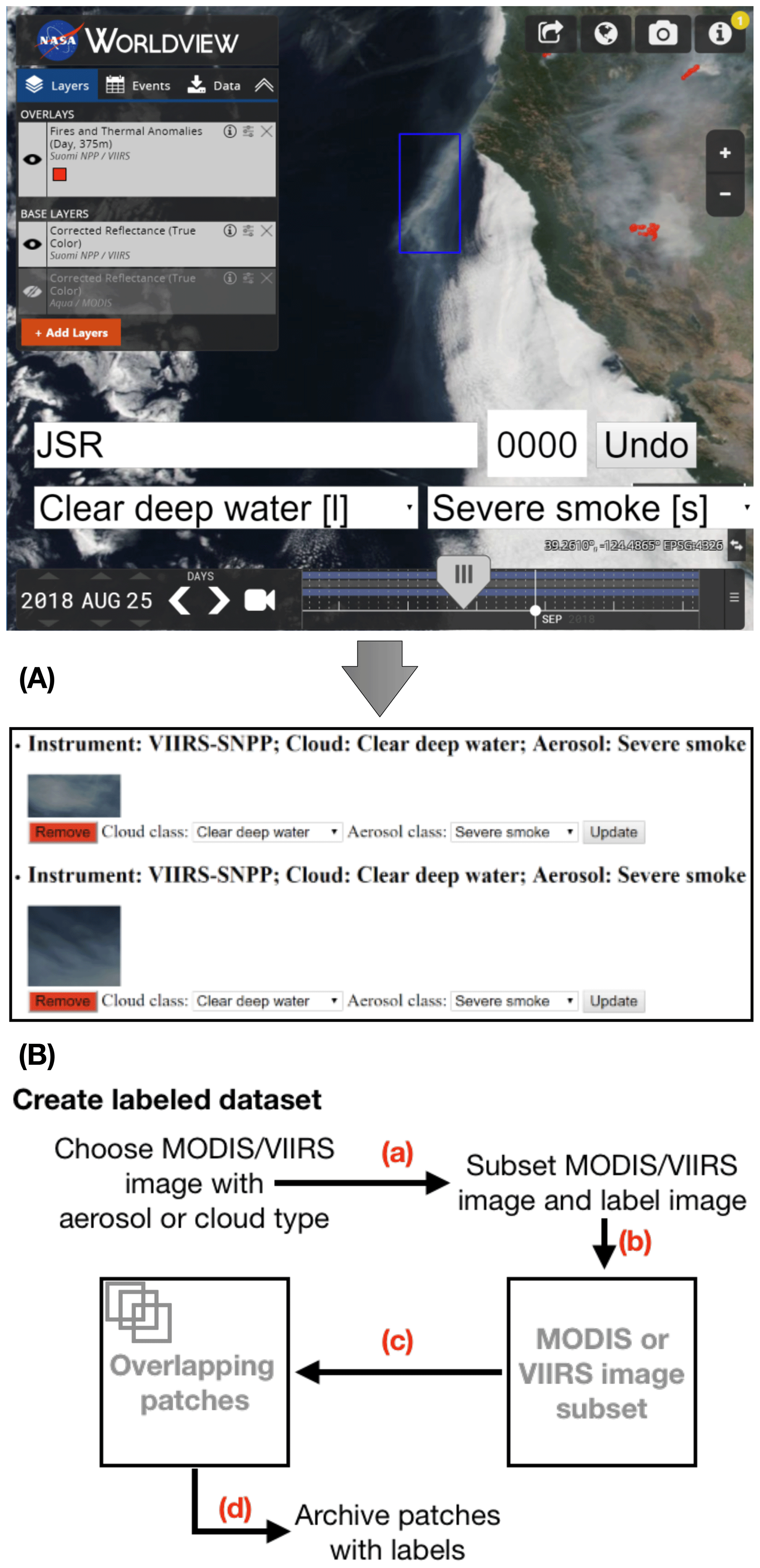
Figure 4(A) The web interface through which a labeled dataset of aerosols and cloud types can be created. First the user decides what to label; e.g., in the above image the user chose to label cumuliform clouds with a dust event. Then the user selects the region of interest (the blue rectangle over the aerosol event) via the mouse cursor; a counter increases (0002) to indicate the labeled image has been archived in a database. (B) To create the labeled dataset (a) a MODIS or VIIRS image is chosen through the web interface, (b) the selected region of interest is used to create a subset of the MODIS or VIIRS image, (c) the subset image is divided into overlapping patches and (d) the patches are archived with the corresponding labels.
In order to ensure consistent labels for the study, one co-author created the labeled dataset (JSR); the system is able to track individual trainers to identify areas of ambiguity. The labeled dataset provides specific cloud and aerosol categories. The cloud categories are (1) clear-air, (2) cirrus/high-altitude, (3) transitional/mixed, (4) closed stratiform, and (5) cumuliform, and the aerosol categories are (1) severe dust, (2) severe smoke and (3) severe pollution. For this study all the aerosol categories are aggregated into one aerosol label; our methodology does not identify specific aerosol types, because the required number of samples in the training dataset increases exponentially as a function of the number of distinct labels the multiclass classifier with the CNN FE algorithm has to identify (Shalev-Shwartz and Ben-David, 2014).
The labeled subset of MODIS–VIIRS images in the datasets was projected onto an equirectangular grid (i.e., equidistant cylindrical map projection) with a spatial resolution of 1 km (i.e., 1 pixel equals 1 km), and each solar reflectance channel was corrected for Rayleigh scattering (Vermote and Vermeulen, 1999).
2.2.1 Training and test datasets
For a specific patch size we created a training dataset by randomly sampling, without replacement, patches from the labeled dataset. The training dataset consists of 75 % of the extracted patches, and the rest of the patches that were not sampled are placed into the test dataset. To prevent a multiclass classifier with an FE algorithm from being biased towards classifying a specific cloud type or aerosol, the random sampling of the patches was carried out such that (1) there are equal portions of patches of each label and (2) there are equal portions of aerosol subtypes (e.g., smoke, dust, pollution; Japkowicz and Stephen, 2002).
2.2.2 Quality assurance of labeled data
To label a subset of a MODIS or VIIRS image through the web interface, as shown in Fig. 4, (1) the cloud and aerosol categories are first chosen and (2) the region of the cloud and aerosol type is selected by dragging a rectangular box over a subset of a MODIS or VIIRS swath which is associated with the cloud and aerosol categories; the MODIS–VIIRS 11 µm band can used to separate high-altitude (cirrus) and low-altitude clouds. To further avoid label inconsistencies in the training dataset two guidelines were followed:
-
The MODIS or VIIRS image subset must only contain the specific cloud and aerosol categories. For example, a subset image must only contain a collection of cumuliform clouds.
-
Except for with cumuliform and cirrus/high-altitude clouds, avoid the inclusion of cloud or aerosol edges wherever possible.
With these guidelines the training dataset excludes examples of cloud and aerosol types that are similar to each other; e.g., cases are avoided where a cloud is equally likely to be transitional/mixed cloud or closed-stratiform cloud.
Further quality assurance (QA) was conducted on the images that were labeled transitional/mixed and cumuliform clouds and aerosols. For a chosen small patch size and a subset MODIS or VIIRS image, cumuliform or transitional/mixed clouds could have in-between regions that are considered clear-air. The MODIS–VIIRS level-2 cloud mask was used to screen out patches within cumuliform or transitional/mixed subset images that are clear-air, since for daytime deep-ocean images the MODIS–VIIRS cloud mask reliably identifies clouds (Frey et al., 2008)1.
2.3 Overview of CNNs in the context of aerosol and cloud-type identification
A set of convolution filters can be used to make distinctions between different image types based on their spatial properties. Based on the response of the filters a decision is made about in what category (i.e., label) the input image belongs. For example, if we want to make a distinction between clear-air and cumuliform cloud images, the output of a high-pass filter would emphasize spatial variation in a cloudy image.
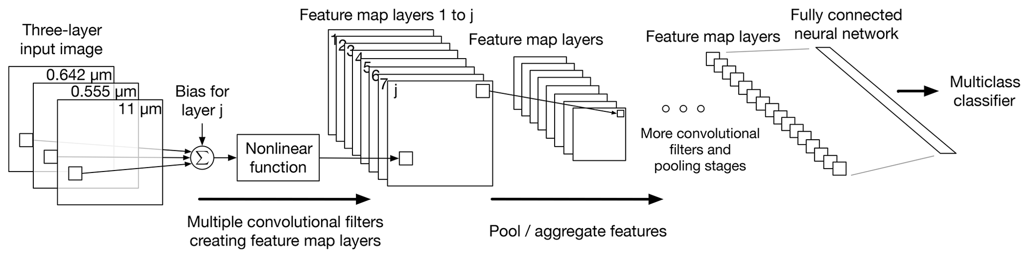
Figure 5A convolutional neural network (CNN) extracts local spatial features from an image and combines the local spatial features to higher-order features. The higher-order features are then used to linearly separate different image types; this figure shows a simplified diagram of a CNN which gives an idea of how the local spatial features and higher-order features are created. In the first CNN layer, after the input image, the CNN has multiple multilayer convolution filters that produce feature maps: for each multilayer filter (1) the CNN convolves the filter with the input image, (2) a bias term specific to the feature map is added to each convolution sum, (3) the results are passed through a nonlinear activation function and (4) the outputs are then placed on a feature map; the nonlinear function with the convolution sums and biases gives the CNN the ability to find the nonlinear separation between different image types. The feature maps produced by the first CNN layer contain local extracted spatial features. The next CNN layer converts the local extracted spatial features into higher-order features by pooling or aggregating the features in each feature map separately using either an averaging or a max operator. The convolution and pooling–aggregation steps are repeated until a series of small feature maps are produced. Depending on the architecture of the CNN, the final layer of feature maps is then passed through a fully connected NN and then finally through a multiclass classifier.
A CNN essentially consists of a series of convolution filters that are tuned to emphasize various spatial properties in an image; each filter produces a feature map. The feature maps are passed through pooling–aggregation (i.e., downsampling) operations that allow a CNN to be less sensitive to shift and distortions of the spatial properties in the images (Simonyan and Zisserman, 2014; LeCun et al., 1989; Krizhevsky et al., 2012; Szegedy et al., 2017; LeCun et al., 1998; LeCun, 1989). More specifically, a CNN extracts local spatial features from an image and combines all the local spatial features to higher-order features via the pooling–aggregation operations, and the higher-order features can be used to make a distinction between different image types; Fig. 5 shows a simplified diagram of a CNN which gives an idea of how the local spatial features and higher-order features are created through the convolutional filters and pooling–aggregation operations.
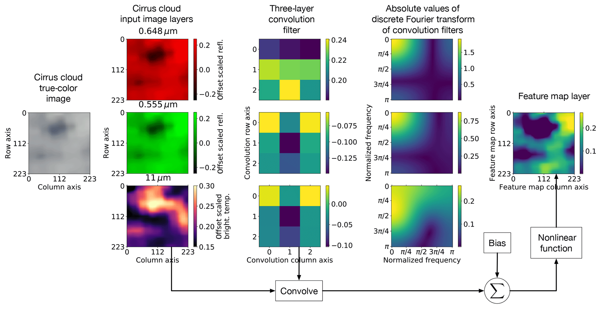
Figure 6This figure shows an example of a feature map that is produced from a cirrus/high-altitude cloud image by a specific 3-dimensional (3D) convolution filter of the first layer of a convolutional neural network (CNN). The layers of the 3D filter are low- and band-pass filters as indicated by the discrete Fourier transforms (DFTs). The 3D convolution filter is convolved over the input image; for each convolution sum a bias term is added and then passed through a nonlinear activation function which corresponds to a feature map pixel. For this example the feature map highlights the local high-reflectivity and clear-air regions in the cirrus/high-altitude cloud.
Similar to fully connected neural networks (NNs), the output of the convolution filters is passed through nonlinear functions (activation functions) with a bias term; the purpose of the nonlinear function with the bias term is to “activate” the output of a convolution filter if the output exceeds some threshold value set by the nonlinear function and bias term. For example, we can emphasize two different levels of variability in an image by connecting a high-pass filter to two ramp functions () with different bias values b; the ramp function basically acts as a threshold function. Figure 6 shows an example of the output of a three-dimensional (3D) convolutional filter that is produced from a cirrus/high-altitude cloud image. Each layer of the 3D filter in Fig. 6 convolves with each corresponding layer of the input image; the discrete Fourier transforms (DFTs) in Fig. 6 show that the filter layers are low- and band-pass filters. With the bias term and nonlinear activation function the 3D filter produces an image that highlights the local high-reflectivity and clear-air regions in the cirrus/high-altitude cloud.
The layers of filters and pooling–aggregation operations with nonlinear activation functions, which produce feature maps, are repeated several times. The last layers of the feature maps are passed through a fully connected NN, and the output is a one-dimensional vector as shown in Fig. 5. The number of consecutive filter and downsampling operations (i.e., depth) increases the expressive power of a CNN (i.e., makes the CNN more accurate). The one-dimensional output vector of a CNN is typically passed through a multiclass classifier that models a probability value of each label for the input image.
Although fully connected NNs have the ability to nonlinearly separate vectors (e.g., images) of different types (Friedman et al., 2001), a fully connected NN is a suboptimal candidate for image recognition tasks since it has no built-in invariance to shifts and distortions in images or structured vectors (LeCun et al., 1998).
Several different CNN configurations have been proposed (Szegedy et al., 2017; Simonyan and Zisserman, 2014); each CNN configuration has different convolution dimension sizes – the number of features maps and the depths differ, the sequence of the convolution and pooling or aggregation differ, etc. It is not clear which CNN configuration is a best choice for a particular image classification problem. In this paper we chose a CNN based on the (1) accuracy ranking of various TensorFlow CNN implementations (Silberman and Guadarrama, 2020) and (2) accessibility of the TensorFlow CNN implementation (Silberman and Guadarrama, 2016).
2.4 Pretrained and fine-tuned CNNs
A CNN that classifies images typically requires a very large labeled training dataset (e.g., a million labeled images) to estimate the parameters of the CNN (i.e., the convolutional filters and bias terms), since the number of parameters required to accurately identify different image types increases exponentially with the size of the input images (Gilton et al., 2020). In this paper the training dataset is relatively small since it is time-consuming to hand-label MODIS–VIIRS images and for optically thick aerosols there are not enough events in the observations.
To address the issue of a small training dataset, we take advantage of a remarkable property of CNNs: if the CNN's convolution filters were tuned (i.e., estimated) on a general set of images (e.g., a wide range of internet images) to make a distinction between image types, the same tuned convolutions filters can be used in the image recognition domain of an entirely different problem. More specifically, the convolution filters in a CNN are kept fixed and the parameters of the multiclass classifier are re-estimated with a training dataset in the new image recognition domain; we call this type of CNN a pretrained CNN. For example, a pretrained CNN that was trained on internet images has been employed successfully in a radar remote-sensing application (Chilson et al., 2019).
The reason why a pretrained CNN's convolutional filters are transferable to a different image recognition domain is (1) concepts of edges and different smoothness properties in images are shared across various image domains, (2) convolutional filters by themselves are agnostic to the image recognition domain since they quantify smoothness properties of images and (3) re-estimation of the multiclass classifier parameters adjust for how the convolution filters respond to the new image recognition domain.
We demonstrate through our results that the method that employs the pretrained CNN feature extractor (FE) can provide accurate classification results, though the classification accuracy is dependent on the patch size.
Since it is not clear whether a pretrained CNN is the best CNN configuration to identify cloud types and optically thick aerosol features, in this paper we also consider a fine-tuned CNN. A fine-tuned CNN is created by (1) taking the pre-estimated convolution filters of a pretrained CNN as initial values, (2) placing the initial values in a new CNN and (3) training the CNN on the training dataset of MODIS–VIIRS images (Sun et al., 2017). In other words, a fine-tuned CNN is basically a pretrained CNN that has been adjusted for another image domain.
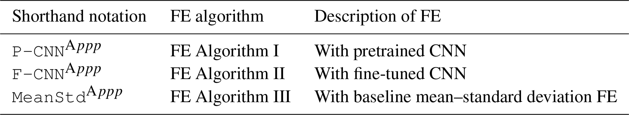
Table 2 shows the shorthand notation of the methods that were used to produce the results; recall that each method, which is created by Algorithm 1, consists of a multiclass classifier with an FE algorithm and Algorithm 2 applies the method on MODIS–VIIRS images.
For example, the shorthand notation P-CNNAppp indicates that the method's multiclass classifier is paired with the pretrained CNN FE algorithm (i.e., FE Algorithm I) which operates on a patch size of ppp by ppp pixels.
Table 2Method mnemonics that are used throughout this results section and the corresponding feature extraction (FE) algorithms.
In our results we seek to answer the following questions:
-
Can our methodology reliably identify optically thick aerosols which the MODIS–VIIRS level-2 products struggle to detect?
-
Can our methodology make a distinction between different cloud types?
-
How well does our methodology label MODIS–VIIRS images that are not part of the training and test datasets? In other words, how well does our methodology generalize?
With the first two questions we qualitatively validate our results with four case studies, since we are unaware of a quantitative dataset to characterize transitional/mixed, closed-stratiform and cumuliform clouds and any dataset that lists aerosol events that the MODIS–VIIRS level-2 products fail to detect. We answer the third question by quantifying cirrus/high-altitude cloud and aerosol identification accuracies as a function of optical depth (OD) by using CALIOP cloud OD and both MODIS and CALIOP aerosol OD (AOD) measurements. Consequently, since we use CALIOP OD measurements to validate our results and because the SNPP VIIRS is not consistently in the same orbit as CALIOP, we only used MODIS-Aqua observations.
3.1 Training, test datasets, and test errors
Recall that two labeled datasets with patch sizes 100 and 25 pixels were created from the adapted NASA Worldview website (see Fig. 4 and Sect. 2.2) and from each labeled dataset training and validation datasets were assembled. Table 3 shows the number of patches in the training and test datasets per patch size and number of unique MODIS–VIIRS image subsets from which the patches were extracted; the quantities in the second column are less than in the third because some images subsets were smaller than 100 pixels by 100 pixels.
Table 3The first two rows show the number of patches in the training and test datasets per patch size. The rest of the rows show the number of unique MODIS–VIIRS image subsets from which the patches were extracted.
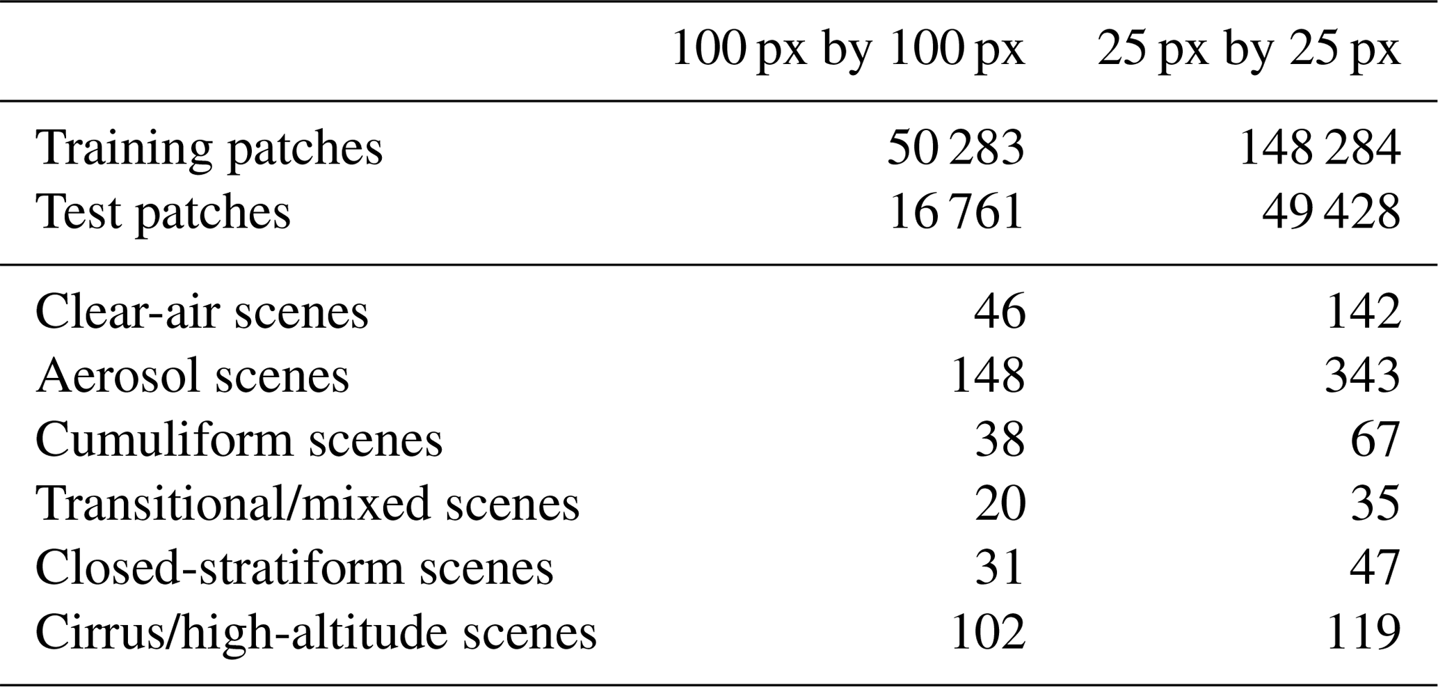
Table 4The test errors of the different methods with different patch sizes. For patch size 25 pixels by 25 pixels the method with the fine-tuned CNN FE algorithm F-CNNA025 has the smallest error. For patch size 100 pixels by 100 pixels the mean–standard deviation FE algorithm MeanStdA100 performs better than the pretrained CNN FE algorithm P-CNNA100. The case studies and sensitivity analyses results, shown elsewhere, demonstrate that F-CNNA025 identifies optically thick aerosols and cirrus clouds at higher accuracies compared to the other methods. The discrepancy between the test errors and what is observed in case studies and sensitivity results indicates that test error is not necessarily an accurate predictor of the out-of-sample (i.e., samples that are not in the training and test datasets) misclassification error.
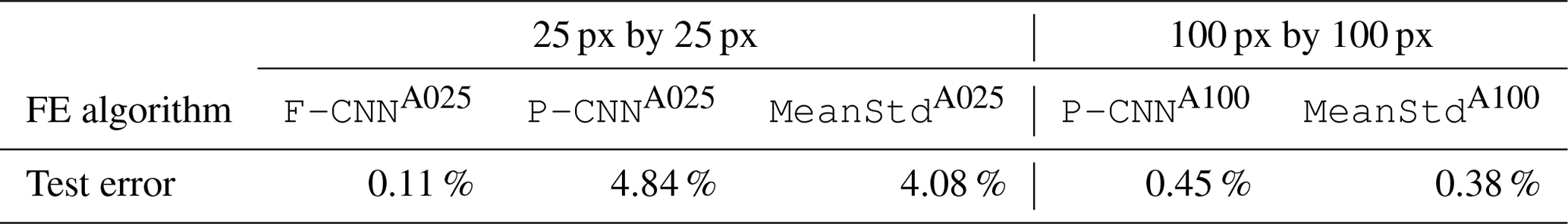
Table 4 shows the test errors of the different methods. The test error is defined as the average number of labeled patches that are misclassified from the test datasets, where the estimated parameters of the methods are independent from the patches in the test datasets. Although the test error is informative in comparing the classification performances of the different methods (Friedman et al., 2001), the test error is not necessarily an accurate predictor of the out-of-sample (i.e., samples that are not in the training and test datasets) misclassification error (Recht et al., 2019).
Table 4 clearly shows that the method with the fine-tuned CNN (i.e., F-CNNA025) has a better error performance compared to the method with a pretrained CNN (i.e., P-CNNA025).
It should be noted that unlike the patches in the training and test datasets that do not contain a mixture of cloud types and aerosols (see Sect. 2.2), patches in MODIS–VIIRS imagery often have a mixture of cloud types. For a patch that contains a mixture of cloud types and/or aerosols, we expect that the methods will label a patch that has the most dominant cloud type or aerosols.
3.2 Case studies
Figures 7, 8, 9 and 10 show four MODIS-Aqua scenes with the labeled results of four methods; we do not show the results of method P-CNNA025 since it has the largest test error. Included in the figures are the true color, 11 µm brightness temperature (BT), and MODIS MYD04 AOD and MODIS MYD35 cloud-mask products (Levy et al., 2013; Frey et al., 2008). The scenes in Figs. 7 and 8 were not part of the training or test datasets, and for all images any sun glint and landmasses have been masked out. The four MODIS-Aqua scenes were specifically chosen because the MYD04 aerosol product has retrievals which are flagged as bad by the MYD04 quality control (QC) and because the MYD35 cloud product labeled the aerosols as clouds (Levy et al., 2013; Frey et al., 2008).
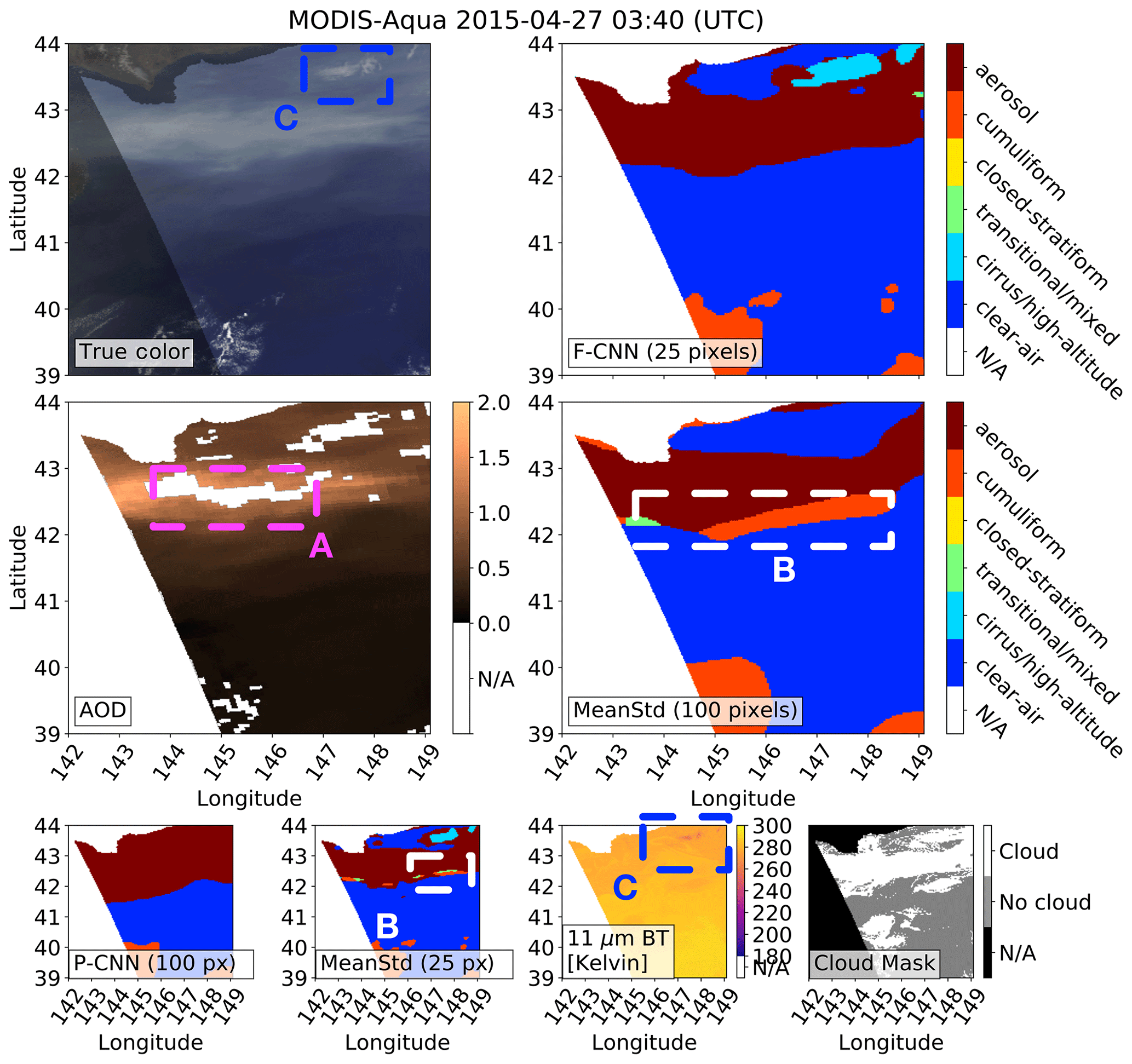
Figure 7Box A shows where (1) the MODIS MYD04 aerosol product has aerosol optical depth (AOD) retrievals which are flagged as bad by the MYD04 quality control, (2) the MODIS MYD35 cloud-mask product labeled the aerosols as clouds, and (3) the pretrained 100-pixel CNN and fine-tuned 25-pixel CNN (F-CNN) methods were able to successfully detect the extreme aerosols. Box B shows where the baseline mean–standard deviation (MeanStd) method misclassified the aerosols as clouds. Box C shows the presence of sparse cirrus/high-altitude clouds with 11 µm brightness temperatures (BTs) ranging between 249 and 257 K and where the 25-pixel methods (F-CNN and MeanStd) were able to detect the cirrus/high-altitude cloud. For all images any sun glint and landmasses have been masked out.
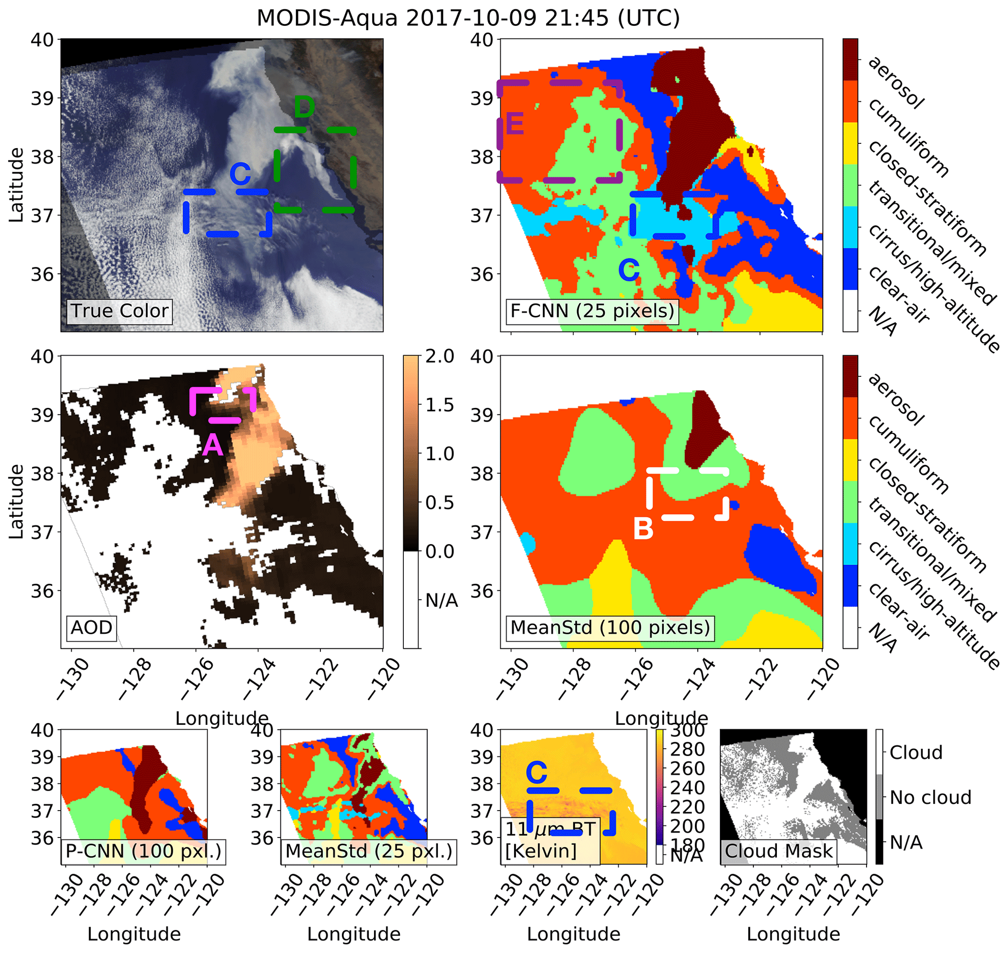
Figure 8Box A shows where (1) the MODIS MYD04 aerosol product has aerosol optical depth (AOD) retrievals which are flagged as bad by the MYD04 quality control, (2) the MODIS MYD35 cloud-mask product labeled the aerosols as clouds, and (3) the pretrained 100-pixel CNN and fine-tuned 25-pixel CNN (F-CNN) methods were able to successfully detect the extreme aerosols. Box B shows where the baseline mean–standard deviation (MeanStd) method misclassified the aerosols as clouds. Box C shows the presence of sparse cirrus/high-altitude clouds with 11 µm brightness temperatures (BTs) ranging between 249 and 257 K and where the 25-pixel methods (F-CNN and MeanStd) were able to detect the cirrus/high-altitude cloud. Box D shows possible closed-stratiform clouds which are near the smoke plume that was detected by the F-CNN method. Box E shows where the F-CNN method separates cumuliform from transitional/mixed clouds. For all images any sun glint and landmasses have been masked out.
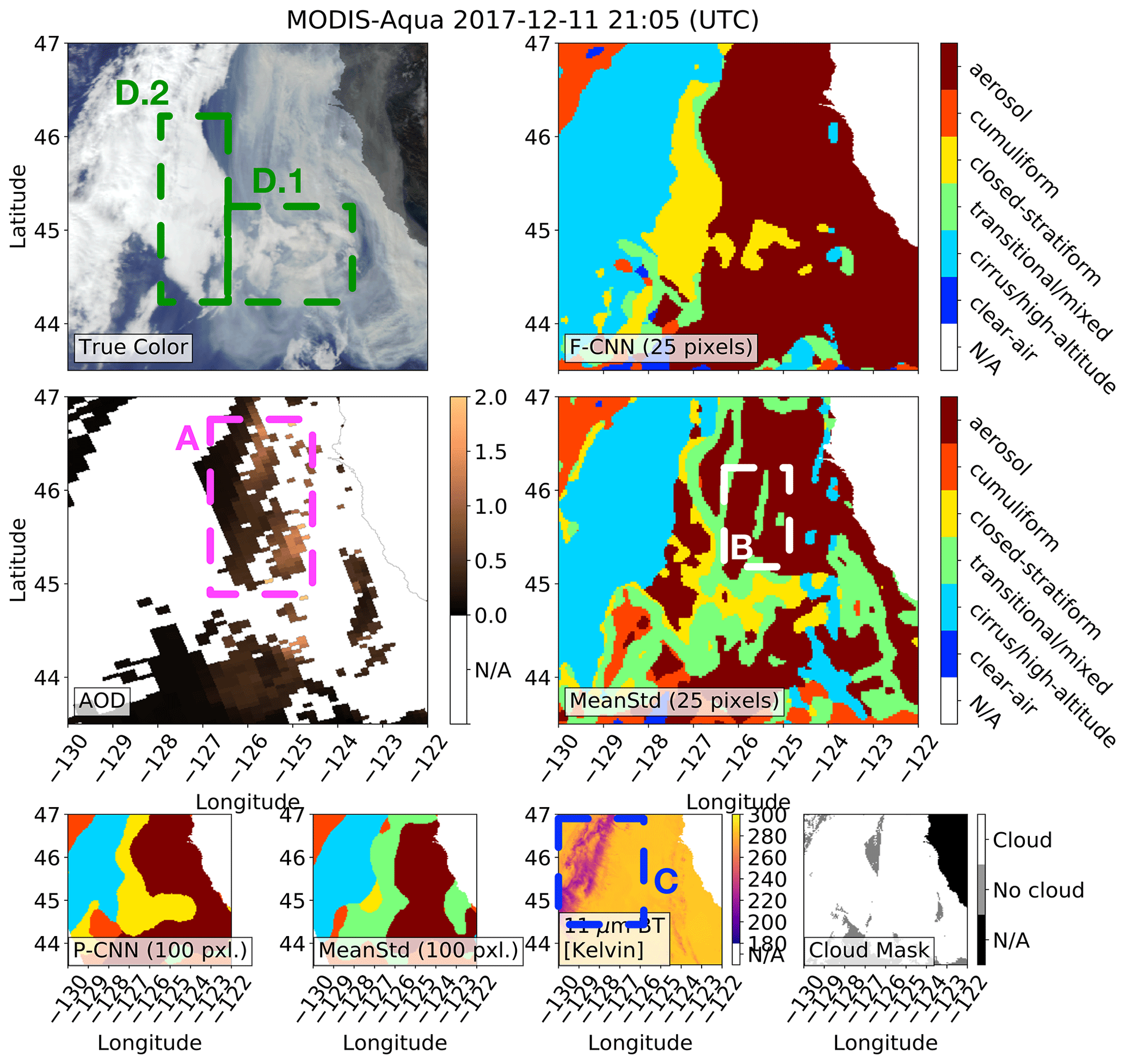
Figure 9Box A shows where (1) the MODIS MYD04 aerosol product has bad aerosol optical depth (AOD) retrievals which are flagged as bad by the MYD04 quality control, (2) the MODIS MYD35 cloud-mask product labeled the aerosols as clouds, and (3) the pretrained 100-pixel CNN and fine-tuned 25-pixel CNN (F-CNN) methods were able to successfully detect the extreme aerosols. Box B shows where the baseline mean–standard deviation (MeanStd) methods misclassified the aerosols as clouds. Box C shows the presence of dense cirrus/high-altitude clouds with 11 µm brightness temperatures (BTs) ranging between 242 and 253 K and where all four methods were able to detect the cirrus/high-altitude cloud. Box D shows possible closed-stratiform clouds which are near or under the smoke plume. All four methods were able to detect the closed-stratiform clouds to various degrees, whereas the 25-pixel methods were able to detect the closed-stratiform clouds at −127 longitude at a finer image resolution compared to the 100-pixel methods. For all images any sun glint and landmasses have been masked out.
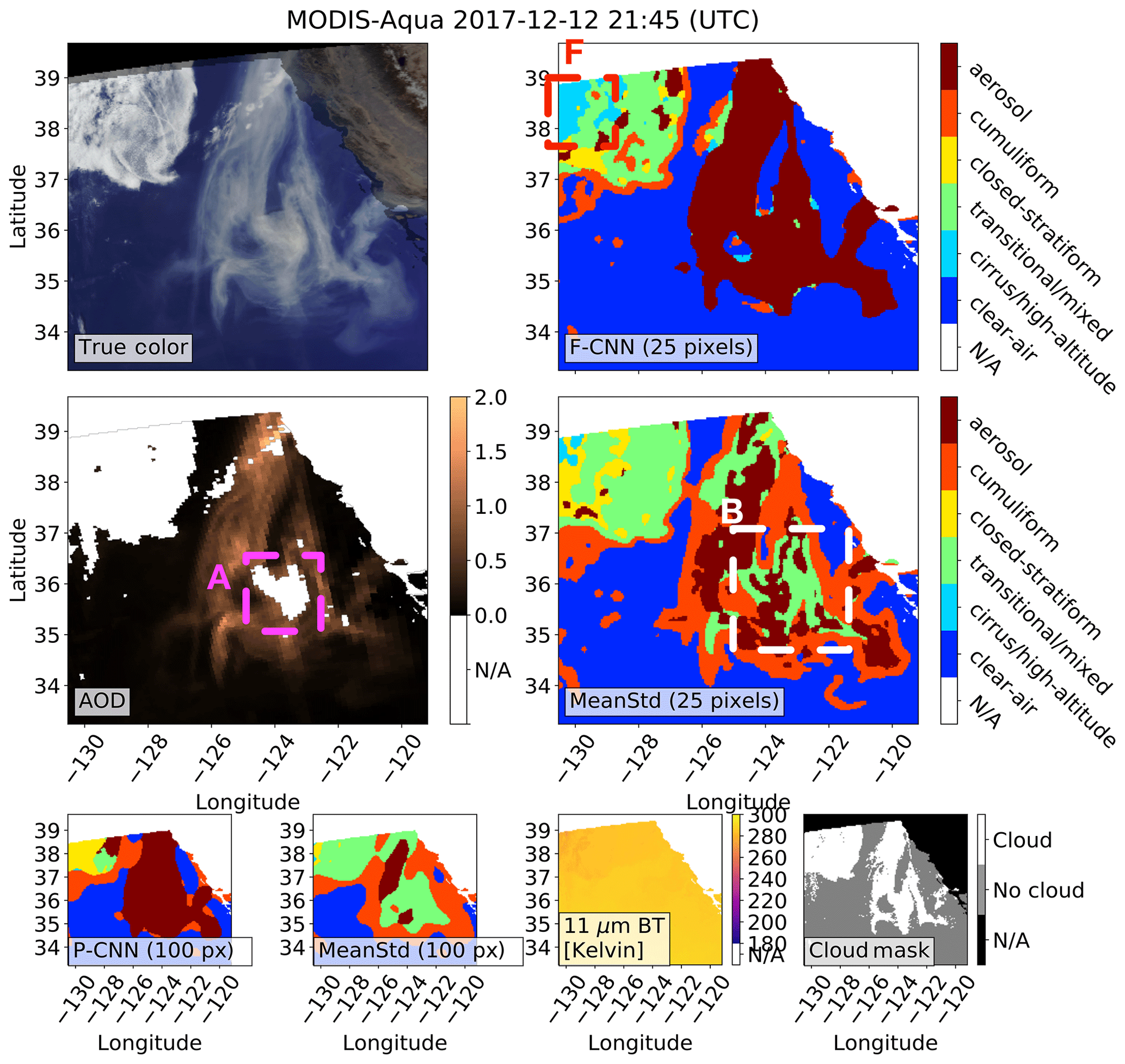
Figure 10Box A shows where (1) the MODIS MYD04 aerosol product has bad aerosol optical depth (AOD) retrievals which are flagged as bad by the MYD04 quality control, (2) the MODIS MYD35 cloud-mask product labeled the aerosols as clouds, and (3) the pretrained 100-pixel CNN and fine-tuned 25-pixel CNN (F-CNN) methods were able to successfully detect the extreme aerosols. Box B shows where the baseline mean–standard deviation (MeanStd) methods misclassified the aerosols as clouds. Box F shows where a part of the clouds were misclassified as cirrus/high-altitude by the F-CNN method, which is possibly due to cirrus/high-altitude-labeled observations in the training dataset that have some contamination of other cloud classes. For all images any sun glint and landmasses have been masked out.
Box A in Figs. 7, 8, 9 and 10 specifically points out where the CNN methods (i.e., F-CNNA025 and P-CNNA100) were able to correctly label the aerosol plumes and the corresponding MYD04 and MYD35 products have bad QC AOD retrievals and the aerosols are labeled as clouds; the CNN methods use the spatial texture differences between aerosols and clouds to make a distinction which enables them to correctly label these optically thick aerosols, where the fine-tuned CNN method is able to identify aerosols at a finer image resolution. In contrast, the baseline methods (i.e., MeanStdA025 and MeanStdA100) misclassify aerosols as clouds in box B in Figs. 7, 8, 9 and 10 because the baseline methods use simple statistics which do not capture the complexity of the spatial texture features of aerosols and cloud types.
The fine-tuned CNN method does misclassify some of the edges of aerosol plumes as cumuliform and cirrus/high-altitude clouds. We did not explicitly model the labeling of the edges of aerosols and clouds, and we consider it part of our future work to improve the labeling of aerosol plume edges. A possible remedy for the misclassified edges is to apply either k-means or spectral clustering to the extracted features of the patches along the edges between the different labels (Shalev-Shwartz and Ben-David, 2014); the labeled edges serve as an initial value of where there might be different cloud types and aerosols, and the cluster method group extracted features of the patches based on how similar they are to each other.
Box C in Figs. 7 and 8 shows the presence of sparse cirrus/high-altitude clouds where the 11 µm BTs range between 249 and 257 K, and in Fig. 9 box C shows dense cirrus/high-altitude clouds that cover a larger area with 11 µm BTs between 242 and 253 K. For the cases where the cirrus/high-altitude clouds are sparser, as in Figs. 7 and 8, the methods with patch size 25 pixels are more sensitive to detecting the cirrus/high-altitude clouds compared to the methods with patch size 100 pixels. In the following subsection we quantify how sensitive the different methods are in detecting the cirrus/high-altitude clouds.
For closed-stratiform, transitional/mixed and cumuliform clouds there is no clear approach to objectively validate the results of the various methods; we point out where these clouds were detected in the case studies with the true-color imagery providing validation. Box D in Figs. 8 and 9 shows possible closed-stratiform clouds which are near or under smoke plumes. In Fig. 8 the fine-tuned CNN method was able to detect the closed-stratiform cloud south of the smoke plume. In Fig. 9 box D.1 shows that a portion of the closed-stratiform cloud is under the smoke plume, and box D.2 shows another closed-stratiform cloud sandwiched between a cirrus/high-altitude cloud and the smoke plume. For box D.1 methods P-CNNA100 and MeanStdA100 identify a larger portion of the closed-stratiform cloud compared to F-CNNA025 and MeanStdA025, since the 25-pixel methods can resolve the closed-stratiform clouds at a higher image resolution which is also evident in box D.2; the baseline methods incorrectly identify more closed-stratiform clouds compared to the other methods.
Box E in Fig. 8 shows where the methods separate cumuliform from transitional/mixed clouds.
Box F in Fig. 10 shows a part of the clouds that were labeled as cirrus/high-altitude by the fine-tuned CNN method where the 11 µm BT is more than 278 K. A possible reason for this misclassification is because the cirrus/high-altitude-labeled observations in the training dataset are contaminated with other cloud types.
3.3 Generalization study through cirrus/high-altitude and aerosol sensitivity analyses
To understand how well our methodology generalizes in labeling MODIS–VIIRS observations that were not part of the training and test datasets, we generated identification accuracy statistics using both the MODIS MYD04 and CALIOP aerosol products and the CALIOP cloud product. Given that the CALIOP spatial footprint is 90 m, only the patches that intersect with the CALIOP footprint were processed by the methods.
3.3.1 Cirrus/high-altitude cloud sensitivity analysis
Figure 11 shows the average fraction of cirrus/high-altitude clouds, per OD interval, detected in the intersection of a CALIOP footprint and patch by the different methods and the MODIS cloud mask (CM) where the CALIOP cloud product indicated that only ice clouds were present. The reported fraction of cirrus/high-altitude cloud statistics is from all of July 2016; CALIOP observations were excluded from the analysis that had water cloud and aerosol observations present at any altitude.
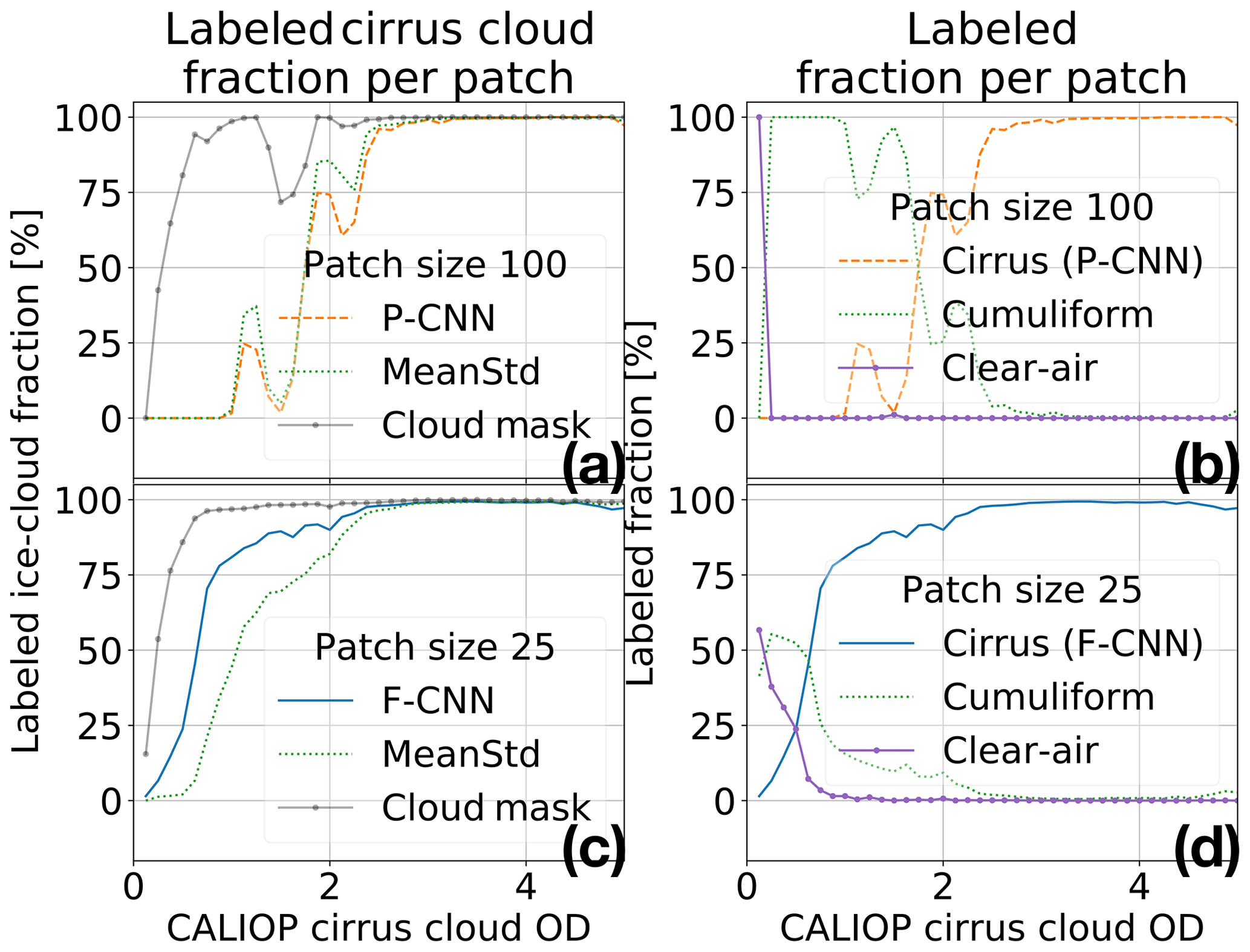
Figure 11For the patches that intersect with the CALIPSO satellite track and the CALIOP cloud product indicating that only ice was present, panels (a) to (d) show the fraction of cirrus/high-altitude clouds detected versus cloud optical depth (OD) in the intersection by the different methods of the proposed methodology and the MODIS cloud mask (CM). Panels (a), (b) and (c), (d) show the fraction of cirrus/high-altitude clouds detected for methods operating on 100- and 25-pixel patches, respectively. Panels (b) and (d) show what the patch intersections were labeled as, versus optical depth, by the pretrained convolutional neural network (P-CNN) and fine-tuned CNN (F-CNN) methods. The MODIS cloud mask in panels (a) and (c) provides a benchmark for detecting clouds.
Figure 11a and c show that the F-CNN method detects cirrus/high-altitude clouds at a higher accuracy compared to the other methods at different patch sizes. Figure 11b and d show that for both patch sizes of 100 and 25 pixels the misclassifications are due to cumuliform clouds, since tenuous cirrus/high-altitude clouds are frequently above cumuliform clouds. At patch size 25 pixels, tenuous cirrus/high-altitude clouds are also prone to misclassification as clear-air as expected. The MODIS cloud mask in Fig. 11a and c provides a benchmark for detecting clouds.
Figure 11a and c show the fraction of cirrus/high-altitude clouds detected by the methods operating on 100- and 25-pixel patches, respectively; the fine-tuned CNN method detects cirrus/high-altitude clouds at a higher accuracy compared to all the other methods. Figure 11b and d give insight as to why the accuracy of detecting cirrus/high-altitude clouds decreases as the cirrus/high-altitude cloud OD decreases. Figure 11b shows that for OD, fewer than three cirrus/high-altitude clouds are typically labeled as cumuliform clouds by the pretrained CNN method. The cumuliform labeling of cirrus/high-altitude clouds should not be regarded as a consistent misclassification, since tenuous cirrus/high-altitude clouds over the ocean are commonly surrounded by cumuliform clouds in a patch size of 100 pixels. Once the patch size decreases to 25 pixels, Fig. 11d shows that the fine-tuned CNN method identifies tenuous cirrus/high-altitude clouds with an OD of less than 1 and are misclassified as clear-air, though cumuliform clouds are still present for cirrus/high-altitude clouds with ODs of up to 3.
3.3.2 Aerosol sensitivity analysis
Figure 12 shows the average fraction of aerosols, per AOD interval, detected in the intersection of a CALIOP footprint and patch by the different methods where the MODIS MYD04 or CALIOP aerosol products indicated that aerosols were present in the complete intersection. The reported fraction of aerosol statistics are from March 2012 up to May 2018, and aerosol observations were excluded from the analysis if (1) any cloud was present according to both the MODIS and CALIOP cloud products and (2) the confidence in the AOD retrieval was less than “high confidence” as indicated by the MYD04 QC.

Figure 12Panels (a) to (d) show the average fraction of aerosols detected in the intersection by the different methods of the proposed methodology for the patches that intersect with the CALIPSO satellite track and either the MODIS MYD04 or the CALIOP aerosol products that indicated there were aerosols present in the complete intersection without any clouds. Panels (a) and (c) show the aerosol fraction versus MODIS MYD04 aerosol optical depth (AOD), and panels (b) and (d) show the aerosol fraction versus CALIOP AOD, where panels (a), (b) and (c), (d) are specific to the methods of patch sizes 100 and 25 pixels, respectively. Panel (e) gives insight as to why the aerosol identification sensitivities relative to MODIS (a, c) and CALIOP (b, d) differ; e.g., for a MYD04 AOD of 0.5, the corresponding CALIOP AOD ranges between 0.25 and 1.25.
Comparing Fig. 12a and b with Fig. 12c and d indicates that methods operating on 100-pixel patches can detect aerosols with a smaller AOD more accurately than methods operating on 25-pixel patches, where the method MeanStd can identify aerosols at a slightly lower AOD compared to the pretrained CNN (P-CNN) and fine-tuned CNN (F-CNN); aerosols that are not identified are typically labeled as clear-air.
In Fig. 12 the insensitivity to detecting tenuous aerosols by the CNN and baseline methods is by design of the training dataset, since the aerosol training data were manually generated from true-color imagery which is not sensitive to thin aerosols. Figure 13 shows histograms of the median MODIS MYD04 aerosol optical depth per patch of the training and test datasets of patch sizes 100 and 25 pixels, specifically for the clear-air and aerosol labels; these histograms indicate a small portion of the training dataset contains tenuous aerosol patches.
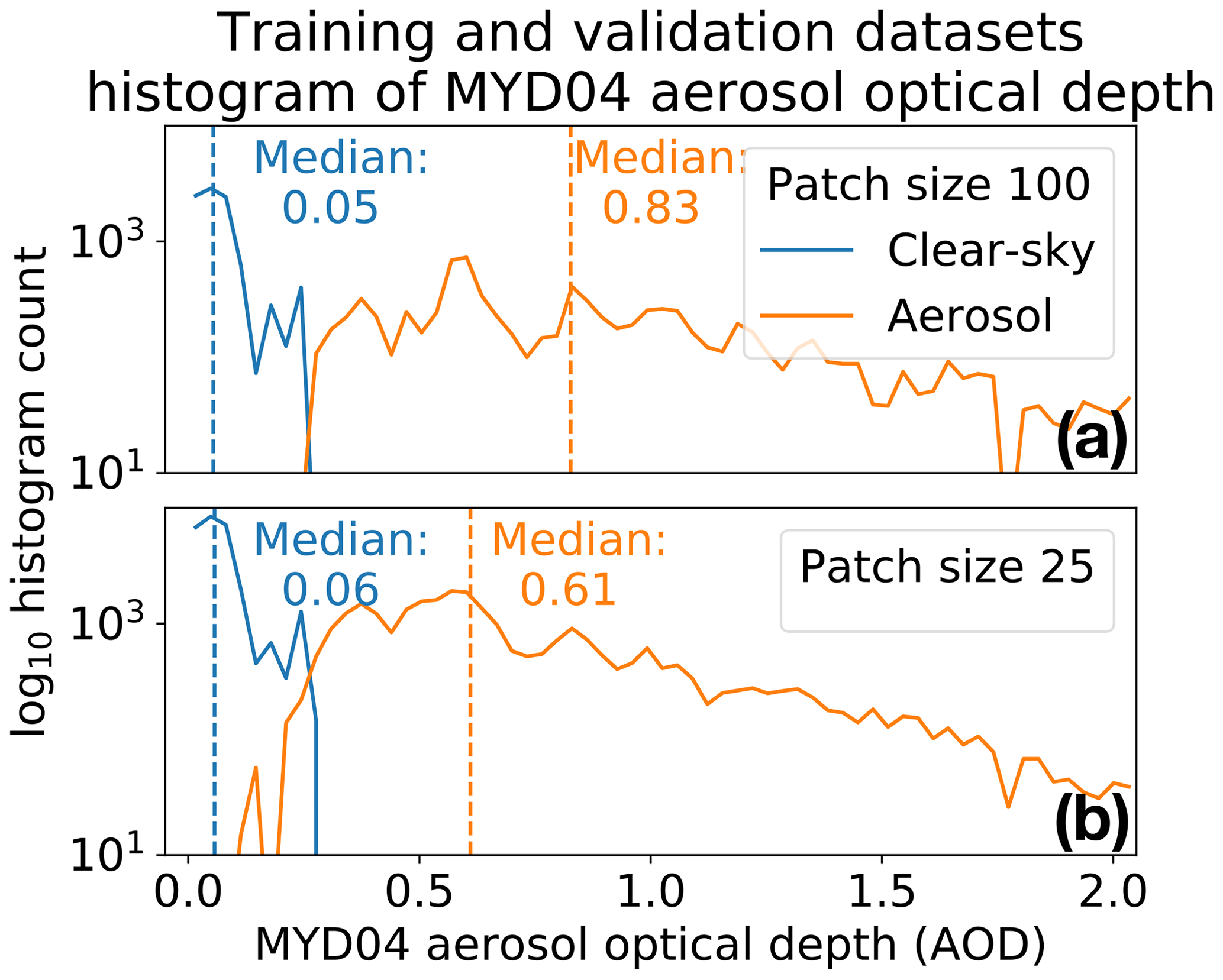
Figure 13Panels (a) and (b) show histograms of the median MODIS MYD04 aerosol optical depth per patch of the training and test datasets of patch sizes 100 and 25 pixels, specifically for the clear-air and aerosol labels. There is a clearer AOD separation between the clear-air and aerosol labels for the (a) 100-pixel patch size datasets compared to that of the (b) 25-pixel patch size.
Figure 12 shows that the sensitivity to detecting aerosols decreases as the patch size decreases, which is an opposite trend compared to the cirrus cloud identification accuracy versus patch size. Figure 13 gives a possible reason why there is a decrease in sensitivity: the AOD distribution of aerosol patches overlaps more with clear-air patches in the 25-pixel patch size training dataset compared to the larger patch size training dataset.
According to Fig. 12a and c the MODIS aerosol product of the proposed methodology can accurately identify optically thick aerosols. However, the CALIOP aerosol product indicates otherwise in Fig. 12b and d. The reason why the proposed methodology's aerosol identification sensitivities relative to MODIS (MYD04) and CALIOP differ could be a discrepancy between the MODIS and CALIOP measured AODs as shown in the two-dimensional histogram in Fig. 12e. For example, for a fixed CALIOP AOD of 2 the corresponding MODIS AOD ranges between 0.25 and 1; in other words, what might be considered optically thick by the CALIOP, could be considered optically thin by the MODIS aerosol product. It is unclear why there is such a large disagreement between the MODIS and CALIOP AODs; there are a couple of studies in which discrepancies between MODIS and CALIOP AODs have been discussed (Kim et al., 2013; Oo and Holz, 2011).
4.1 Summary
We introduced a new methodology that identifies distinct cloud types and optically thick aerosols by leveraging spatial textual features from radiometer images that are extracted via CNNs. We demonstrated the following through several case studies and via comparisons of the MODIS and CALIOP cloud and aerosol products:
-
The proposed methodology can identify low-level to midlevel cumuliform, closed-stratiform, transitional/mixed (transitional between the two or mixed types) or cirrus/high-altitude cloud types; these cloud regimes are related to meteorological conditions due to the strong correlations between cloud types and atmospheric dynamics (Levy et al., 2013; Tselioudis et al., 2013; Evan et al., 2006; Jakob et al., 2005; Holz, 2002).
-
The detection accuracy of the cirrus/high-altitude cloud type is a strong function of the image patch size, where a smaller patch size yields higher accuracy. We found that cirrus/high-altitude clouds are often misclassified as clear-air and cumuliform clouds, resulting from the frequent cumuliform clouds beneath tenuous cirrus clouds.
-
The proposed methodology can reliably identify these optically thick aerosol events, whereas the MODIS level-2 aerosol product labeled the AOD retrievals of the optically thick aerosols as bad with the quality control flags (Levy et al., 2013). The implication of relying on the MODIS level-2 aerosol product quality control in a climatological research project involving aerosols is that most of the large-impact optically thick aerosols will be excluded in the research study; this problem stresses the importance of the reliable identification of optically thick aerosols.
-
Optically thick aerosol detection is also a strong function of the image patch size, where smaller patch sizes yield lower accuracy. The insensitivity to tenuous aerosols is by design, since the human-labeled training dataset only contained optically thick aerosols. For future work we will consider increasing the number of lower AOD aerosol-labeled images in the labeled dataset in order to increase the aerosol detection sensitivity.
Unfortunately, since we do not know of any dataset of labeled cumuliform, closed-stratiform and transitional/mixed clouds, there was no clear approach to quantifying the detection accuracy of these clouds; we leave it to future work to characterize this accuracy performance.
A surprising aspect of our methodology is that the CNNs that we employ are pretrained on nonradiometer images (e.g., random images from the internet). In more detail, the convolutional filters of the CNNs which extract the spatial textual features from images were estimated from nonradiometer images; employing pretrained CNNs in other remote-sensing problems with promising results has been recently reported in the literature (Chilson et al., 2019). We demonstrated in this paper that with additional fine-tuning of a pretrained CNN, by further estimating the convolutional filters where the initial values are of a pretrained CNN, the classification performance of radiometer images can be further improved upon.
4.2 Future work
Our proposed methodology is considered preliminary work, and further work will be required to maximize the methodology's operation and scientific use. The current limitations are that (1) the methodology is computationally inefficient, (2) cloud type and aerosols are only identified over deep-ocean images, and (3) the methodology only operates on daytime observations. Currently a total of 20 min is required to label a MODIS 5 min granule with a GPU-accelerated fine-tuned CNN method. This computational inefficiency is because each image patch is processed independently from the other patches although the patches overlap. Consequently, the CNN convolutional operations on each pixel are repeated several times. This computational redundancy can be eliminated by adapting the CNN architecture, and potential computational speed can be increased at least by a factor of 5.
We consider the deep-ocean and daytime-only limitations as future research directions. Cloud-type and aerosol identification over land is a much harder research problem since the Earth's surface is nonuniform and changes over time; in our future work we plan to model the Earth's surface and incorporate the land-surface model into our CNN methodology. In regard to the daytime-only limitation, the CNN methods in the paper have only been applied to three spectral channels (0.642, 0.555 and 11 µm) and it would be interesting to understand how the cloud-type and aerosol identification accuracies change when some spectral bands are removed or added from the input images. For example, how would the CNN identification accuracies be impacted if only infrared-radiance measurements were used?
Another future research direction is how to adapt our methodology to geostationary Earth-orbiting (GEO) imagers. GEO imagers provide temporal multispectral image sequences where the temporal resolution is at least 10 min. A compelling research question would be the following: how can we leverage the temporal component of the GEO images to identify cloud types and aerosols while incorporating cloud and aerosol physical models into the machine learning methodology? The temporal information content will allow the machine learning to separate high-altitude from low-altitude clouds, while the cloud and aerosol physical models will provide additional information that can constrain the cloud-type and aerosol identification.
A1 Algorithm 1 – estimate method parameters – training phase
Algorithm 1 shows a detailed outline of the training-phase algorithm. Suppose the number of labeled patches in the training and test datasets are K and L, respectively, the labeled training and test datasets are denoted by and , respectively; the superscripts (k) and (l) are indices to the labeled patches in the training and test dataset, respectively. Each patch, denoted by a 3-dimensional tensor , has three layers and covers an area of S by S pixels. The corresponding label vector Y∈ℝ6 is a six-element canonical vector (i.e., ith vector equals 1 and the rest are zero) where the position of the one-element corresponds to the categories of clear-air, optically thick aerosol features, cumuliform clouds, transitional clouds, closed-stratiform clouds or cirrus/high-altitude clouds.
For each patch in the training dataset the FE algorithm creates element feature vectors denoted by . The probability value of a feature vector Z being of label Y is modeled by a normalized exponential function:
where is the parameter of the multinomial classifier which linearly weights the feature vector Z, the label vector Y selects the column of W that is multiplied with the feature vector Z and ei∈ℝ6 is a six-element canonical vector.
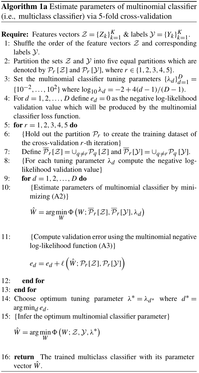
Algorithm 1 employs Algorithm 1a to estimate the optimum weight matrix W. In more detail, with the training features and label vectors and , Algorithm 1a estimates the weight matrix W by minimizing the objective function:
where Eq. (A3) is the negative log-likelihood (i.e., loss) function and λ>0 is the regularizer (i.e., tuning) parameter of the l2 penalty term as indicated in Eq. (A2). The optimum tuning parameter λ is estimated by Algorithm 1a using 5-fold cross validation (Friedman et al., 2001), where for each tuning parameter a validation error is computed and the optimum tuning parameter corresponds to the smallest validation error; the validation error is computed using the loss function (A3).
A patch is labeled with the function
where
which produces a label vector by finding the canonical vector ei that maximizes the modeled probability (A1) with the extracted feature vector Z and estimated weight matrix .
For a given test datasets of feature and label vectors, the test error is computed by
where is number of label vectors and Indc{⋅} is an indicator function defined as
Algorithm 1 assumes that the parameters of the CNN FE algorithm are already estimated. Hence, the parameters of the fine-tuned CNN are estimated separately from Algorithm 1 with the same training dataset that is used by Algorithm 1; the fine-tuning is accomplished using a software package such as TensorFlow (Abadi et al., 2016). The software package scikit-learn can be used to minimize the objective function (A2) (Pedregosa et al., 2011).
A2 Algorithm 2 – applying trained method to label a MODIS or VIIRS image
Algorithm 2 shows a detailed outline of how a method is applied on a MODIS or VIIRS image.
B1 Pretrained CNN feature extractor
FE Algorithm I gives an outline of the pretrained CNN FE algorithm. The pretrained CNN that is used is the Inception-v4 CNN (Szegedy et al., 2017).
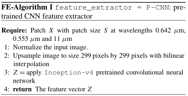
In FE Algorithm I the input image is normalized such that each pixel for the average input image has a zero mean and a standard deviation of 1. The Inception-v4 CNN was trained on normalized images to improve performance (Orr and Müller, 2003, chap. 1). The coefficients that are used to normalize the input image are computed from the training dataset. The Inception-v4 CNN takes as input images with size 299 pixels by 299 pixels; hence the MODIS–VIIRS image patches are upsampled using bilinear interpolation.
B2 Fine-tuned CNN feature extractor
FE Algorithm II gives an outline of the fine-tuned CNN FE. The pretrained VGG-16 CNN was chosen as the basis of the fine-tuned CNN rather than a pretrained Inception-v4, since VGG-16 has fewer parameters (i.e., degrees of freedom) compared to that of the Inception-v4 CNN. The parameters of the fine-tuned VGG-16 CNN are estimated separately from Algorithm 1 with the same training dataset that is used by Algorithm 1; the fine-tuning is accomplished using a software package such as TensorFlow (Abadi et al., 2016). As with the Inception-v4 CNN the input image to the fine-tuned VGG-16 CNN is normalized. The VGG-16 CNN takes as input images with size 224 pixels by 224 pixels; hence the MODIS–VIIRS image patches are upsampled using bilinear interpolation.
B3 Mean–standard deviation feature extractor
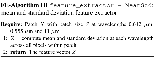
FE Algorithm III gives an outline of the mean and standard deviation FE; for a given patch, FE Algorithm III computes for each input wavelength the mean and standard deviation (SD) across all pixels, and the mean and SD values per wavelength are placed in a six-element vector.
This paper uses observations of the MODIS, VIIRS and CALIOP satellite instruments. MODIS and VIIRS are passive radiometers which measure the solar reflectances and infrared emissions of the Earth and its atmosphere (Marchant et al., 2016; Salomonson et al., 1989; Platnick et al., 2016). The advantage of MODIS and VIIRS observations is that they cover large spatial areas, though from these passive measurements it is hard to identify tenuous clouds and aerosols. In comparison CALIOP is an active lidar instrument which makes direct measurements of cloud and aerosols at higher sensitivities compared to passive instruments (Liu et al., 2005; Young et al., 2008), though the CALIOP observations cover a smaller spatial area compared to MODIS and VIIRS.
Publicly available software were used to produce the results in this paper. TensorFlow was used to for the convolutional neural networks (CNNs), and the pretrained models are available at https://github.com/tensorflow/models/tree/master/research/slim (Silberman and Guadarrama, 2020). The software package scikit-learn was used to model the multinomial classifier (Pedregosa et al., 2011) (https://www.jmlr.org/papers/volume12/pedregosa11a/pedregosa11a.pdf, last access: 8 October 2020).
All data used in this study are publicly available. The MODIS and VIIRS data are available through the NASA Level-1 and Atmosphere Archive and Distribution System Web Interface (https://ladsweb.modaps.eosdis.nasa.gov/, last access: 16 January 2020, NASA, 2020). The CALIOP data were obtained from the NASA Langley Research Center Atmospheric Science Data Center (https://www-calipso.larc.nasa.gov, last access: 8 October 2020, NASA Langley Research Center ASDC, 2020).
RMW and WJM developed the statistical image processing methodologies. JSR created the labeled datasets. REH provided expert advice on MODIS, VIIRS and CALIOP datasets. All authors participated in the writing of the manuscript.
The authors declare that they have no conflict of interest.
We would like to thank Davis Gilton for his thoughtful suggestions on fine-tuning CNNs. We would also like to thank the reviewers for their thoughtful feedback.
This research has been supported by the ONR-322 (grant no. N00173-19-1-G005), DOE (grant no. DE‐AC02‐06CH11357) and National Science Foundation (NSF; grant nos. OAC‐1934637 and DMS‐1930049).
This paper was edited by Alexander Kokhanovsky and reviewed by two anonymous referees.
Abadi, M., Agarwal, A., Barham, P., Brevdo, E., Chen, Z., Citro, C., Corrado, G. S., Davis, A., Dean, J., Devin, M., Ghemawat, S., Goodfellow, I. J., Harp, A., Irving, G., Isard, M., Jia, Y., Józefow-icz, R., Kaiser, L., Kudlur, M., Levenberg, J., Mané, D., Monga, R., Moore, S., Murray, D. G., Olah, C., Schuster, M., Shlens, J.,Steiner, B., Sutskever, I., Talwar, K., Tucker, P. A., Vanhoucke,V., Vasudevan, V., Viégas, F. B., Vinyals, O., Warden, P., Wattenberg, M., Wicke, M., Yu, Y., and Zheng, X.: : Tensorflow: Large-scale machine learning on heterogeneous distributed systems, arXiv [preprint], arXiv:1603.04467, 14 March 2016. a, b
Al-Saadi, J., Szykman, J., Pierce, R. B., Kittaka, C., Neil, D., Chu, D. A., Remer, L., Gumley, L., Prins, E., Weinstock, L., Wayland, R., Dimmick, F., and Fishman, J.: Improving national air quality forecasts with satellite aerosol observations, B. Am. Meteorol. Soc., 86, 1249–1262, 2005. a
Blackwell, W. J.: A neural-network technique for the retrieval of atmospheric temperature and moisture profiles from high spectral resolution sounding data, IEEE T. Geosci. Remote, 43, 2535–2546, 2005. a
Boukabara, S.-A., Krasnopolsky, V., Stewart, J. Q., Maddy, E. S., Shahroudi, N., and Hoffman, R. N.: Leveraging Modern Artificial Intelligence for Remote Sensing and NWP: Benefits and Challenges, B. Am. Meteorol. Soc., 100, ES473–ES491, 2019. a
Chilson, C., Avery, K., McGovern, A., Bridge, E., Sheldon, D., and Kelly, J.: Automated detection of bird roosts using NEXRAD radar data and Convolutional neural networks, Remote Sensing in Ecology and Conservation, 5, 20–32, 2019. a, b
Evan, A. T., Dunion, J., Foley, J. A., Heidinger, A. K., and Velden, C. S.: New evidence for a relationship between Atlantic tropical cyclone activity and African dust outbreaks, Geophys. Res. Lett., 33, L19813, https://doi.org/10.1029/2006GL026408, 2006. a, b
Frey, R. A., Ackerman, S. A., Liu, Y., Strabala, K. I., Zhang, H., Key, J. R., and Wang, X.: Cloud detection with MODIS. Part I: Improvements in the MODIS cloud mask for collection 5, J. Atmos. Ocean. Tech., 25, 1057–1072, 2008. a, b, c
Friedman, J., Hastie, T., and Tibshirani, R.: The elements of statistical learning, vol. 1, Springer series in statistics, New York, USA, 2001. a, b, c, d, e, f, g, h
Gagne II, D. J., Haupt, S. E., Nychka, D. W., and Thompson, G.: Interpretable deep learning for spatial analysis of severe hailstorms, Mon. Weather Rev., 147, 2827–2845, 2019. a
Gilton, D., Ongie, G., and Willett, R.: Neumann Networks for Linear Inverse Problems in Imaging, IEEE Transactions on Computational Imaging, 6, 328–343, https://doi.org/10.1109/TCI.2019.2948732, 2020. a
Heidinger, A. K., Foster, M., Botambekov, D., Hiley, M., Walther,A., and Li, Y.: Using the NASA EOS A-Train to Probe the Performance of the NOAA PATMOS-x Cloud Fraction CDR, Remote Sensing, 8, 511, https://doi.org/10.3390/rs8060511, 2016. a
Heidinger, A. K., Evan, A. T., Foster, M. J., and Walther, A.: A naive Bayesian cloud-detection scheme derived from CALIPSO and applied within PATMOS-x, J. Appl. Meteorol. Clim., 51, 1129–1144, 2012. a
Holz, R. E.: Measurements of cirrus backscatter phase functions using a high spectral resolution lidar, Master's thesis, University of Wisconsin–Madison, 2002. a, b
Jakob, C., Tselioudis, G., and Hume, T.: The radiative, cloud, and thermodynamic properties of the major tropical western Pacific cloud regimes, J. Climate, 18, 1203–1215, 2005. a, b
Japkowicz, N. and Stephen, S.: The class imbalance problem: A systematic study, Intelligent Data Analysis, 6, 429–449, 2002. a
Kim, M.-H., Kim, S.-W., Yoon, S.-C., and Omar, A. H.: Comparison of aerosol optical depth between CALIOP and MODIS-Aqua for CALIOP aerosol subtypes over the ocean, J. Geophys. Res.-Atmos., 118, 13–241, 2013. a, b
Klaes, K. D., Montagner, F., and Larigauderie, C.: Metop-B, the second satellite of the EUMETSAT polar system, in orbit, in: Earth Observing Systems XVIII, International Society for Optics and Photonics, vol. 8866, p. 886613, 2013. a
Krishnapuram, B., Carin, L., Figueiredo, M. A., and Hartemink, A. J.: Sparse multinomial logistic regression: Fast algorithms and generalization bounds, IEEE T. Pattern Anal., 27, 957–968, 2005. a, b, c
Krizhevsky, A., Sutskever, I., and Hinton, G. E.: ImageNet Classification with Deep Convolutional Neural Networks, in: Advances in Neural Information Processing Systems 25 (NIPS 2012), edited by: Pereira, F., Burges, C. J. C., Bottou, L., and Weinberger, K. Q., Curran Associates, Inc., 1097–1105, 2012. a, b
LeCun, Y.: Generalization and network design strategies, Tech. Rep. CRG-TR-89-4, Department of Computer Science, University of Toronto, Toronto, Canada, 1989. a, b
LeCun, Y., Boser, B., Denker, J. S., Henderson, D., Howard, R. E., Hubbard, W., and Jackel, L. D.: Backpropagation applied to handwritten zip code recognition, Neural Comput., 1, 541–551, 1989. a, b
LeCun, Y., Bottou, L., Bengio, Y., Haffner, P.: Gradient-based learning applied to document recognition, P. IEEE, 86, 2278–2324, 1998. a, b, c
Leinonen, J., Guillaume, A., and Yuan, T.: Reconstruction of Cloud Vertical Structure with a Generative Adversarial Network, Geophys. Res. Lett., 46, 7035–7044, 2019. a
Levy, R. C., Mattoo, S., Munchak, L. A., Remer, L. A., Sayer, A. M., Patadia, F., and Hsu, N. C.: The Collection 6 MODIS aerosol products over land and ocean, Atmos. Meas. Tech., 6, 2989–3034, https://doi.org/10.5194/amt-6-2989-2013, 2013. a, b, c, d, e, f, g
Liu, Z., Omar, A., Hu, Y., Vaughan, M., and Winker, D.: CALIOP algorithm theoretical basis document–Part 3: Scene classification algorithms, Tech. Rep. PC-SCI-202 Part 3, NASA Langley Research Center, NASA Langley Research Center, Hampton, Virginia, USA, 2005. a
Marchant, B., Platnick, S., Meyer, K., Arnold, G. T., and Riedi, J.: MODIS Collection 6 shortwave-derived cloud phase classification algorithm and comparisons with CALIOP, Atmos. Meas. Tech., 9, 1587–1599, https://doi.org/10.5194/amt-9-1587-2016, 2016. a
Merchant, C., Harris, A., Maturi, E., and MacCallum, S.: Probabilistic physically based cloud screening of satellite infrared imagery for operational sea surface temperature retrieval, Q. J. Roy. Meteor. Soc., 131, 2735–2755, 2005. a
Minnis, P., Hong, G., Sun-Mack, S., Smith Jr, W. L., Chen, Y., and Miller, S. D.: Estimating nocturnal opaque ice cloud optical depth from MODIS multispectral infrared radiances using a neural network method, J. Geophys. Res.-Atmos., 121, 4907–4932, 2016. a
Molod, A., Takacs, L., Suarez, M., Bacmeister, J., Song, I.-S., and Eichmann, A.: The GEOS-5 atmospheric general circulation model: Mean climate and development from MERRA to Fortuna, Tech. Rep. NASA/TM-2012-104606, NASA, GoddardSpace Flight Center Greenbelt, Maryland, USA, 2012. a
NASA: NASA Earth Science Data, available at: https://earthdata.nasa.gov, last access: 16 January 2020. a, b
NASA Langley Research Center ASDC: The Cloud-Aerosol Lidar and Infrared Pathfinder Satellite Observation (CALIPSO), NASA, available at: https://www-calipso.larc.nasa.gov, last access: 8 October 2020. a
Oo, M. and Holz, R.: Improving the CALIOP aerosol optical depth using combined MODIS-CALIOP observations and CALIOP integrated attenuated total color ratio, J. Geophys. Res., 116, D14201, https://doi.org/10.1029/2010JD014894, 2011. a
Orr, G. B. and Müller, K. R.: Neural networks: tricks of the trade, Springer, Berlin, Heidelberg, 2003. a
Parkinson, C. L.: Summarizing the first ten years of NASA's Aqua mission, IEEE J. Sel. Top. Appl., 6, 1179–1188, 2013. a
Pavolonis, M. J., Sieglaff, J., and Cintineo, J.: Spectrally Enhanced Cloud Objects – A generalized framework for automated detection of volcanic ash and dust clouds using passive satellite measurements: 1. Multispectral analysis, J. Geophys. Res.-Atmos., 120, 7813–7841, 2015. a
Pedregosa, F., Varoquaux, G., Gramfort, A., Michel, V., Thirion, B., Grisel, O., Blondel, M., Prettenhofer, P., Weiss, R., Dubourg, V., Vanderplas, J., Passos, A., Cournapeau, D., Brucher, M., Perrot, M., and Duchesnay, E.: Scikit-learn: Machine Learning in Python, J. Mach. Learn. Res., 12, 2825–2830, available at: https://www.jmlr.org/papers/volume12/pedregosa11a/pedregosa11a.pdf (last access: 8 October 2020), 2011. a, b
Platnick, S., Meyer, K. G., King, M. D., Wind, G., Amarasinghe, N., Marchant, B., Arnold, G. T., Zhang, Z., Hubanks, P. A., Holz, R. E., Yang, P., Ridgway, W. L., and Riedi, J.: The MODIS cloud optical and microphysical products: Collection 6 updates and examples from Terra and Aqua, IEEE T. Geosci. Remote, 55, 502–525, 2016. a, b, c
Recht, B., Roelofs, R., Schmidt, L., and Shankar, V.: Do ImageNet Classifiers Generalize to ImageNet?, arXiv [preprint], arXiv:1902.10811, 13 February 2019. a
Salomonson, V. V., Barnes, W., Maymon, P. W., Montgomery, H. E., and Ostrow, H.: MODIS: Advanced facility instrument for studies of the Earth as a system, IEEE T. Geosci. Remote, 27, 145–153, 1989. a, b
Schueler, C. F., Clement, J. E., Ardanuy, P. E., Welsch, C., DeLuccia, F., and Swenson, H.: NPOESS VIIRS sensor design overview, in: Earth Observing Systems VI, International Society for Optics and Photonics, vol. 4483, 11–23, 2002. a
Shalev-Shwartz, S. and Ben-David, S.: Understanding MachineLearning: From Theory to Algorithms, Cambridge University Press, https://doi.org/10.1017/CBO9781107298019, 2014. a, b
Silberman, N. and Guadarrama, S.: Tensorflow-slim image classification model library, https://github.com/tensorflow/models/tree/master/research/slim, last access: 16 January 2016. a
Silberman, N. and Guadarrama, S.: TensorFlow-Slim image classification model library, available at: https://github.com/tensorflow/models/tree/master/research/slim, last access: 16 January 2020. a, b
Simonyan, K. and Zisserman, A.: Very deep convolutional networks for large-scale image recognition, arXiv [preprint], arXiv:1409.1556, 4 September 2014. a, b, c, d
Stephens, G. L., Vane, D. G., Boain, R. J., Mace, G. G., Sassen, K., Wang, Z., Illingworth, A. J., O'connor, E. J., Rossow, W. B., Durden, S. L., Miller, S. D., Austin, R. T., Benedetti, A., Mitrescu, C., and the CloudSat Science Team: The CloudSat mission and the A-Train: A new dimension of space-based observations of clouds and precipitation, B. Am. Meteorol. Soc., 83, 1771–1790, 2002. a
Sun, C., Shrivastava, A., Singh, S., and Gupta, Revisiting Unreasonable Effectiveness of Data in Deep Learning Era, in: Proceedings of the IEEE International Conference on Computer Vision (ICCV), 843–852, 2017. a
Szegedy, C., Ioffe, S., and Vanhoucke, V.: Inception-v4, Inception-ResNet and the Impact of Residual Connections on Learning,CoRR, abs/1602.07261, https://doi.org/http://arxiv.org/abs/1602.07261, 2016. a, b, c, d
Takenaka, H., Nakajima, T. Y., Higurashi, A., Higuchi, A., Takamura, T., Pinker, R. T., and Nakajima, T.: Estimation of solar radiation using a neural network based on radiative transfer, J. Geophys. Res., 116, D08215, https://doi.org/10.1029/2009JD013337, 2011. a
Tselioudis, G., Rossow, W., Zhang, Y., and Konsta, D.: Global weather states and their properties from passive and active satellite cloud retrievals, J. Climate, 26, 7734–7746, 2013. a, b, c
Vermote, E. and Vermeulen, A.: Atmospheric correction algorithm: spectral reflectances (MOD09), Tech. Rep., NASA con-tract NAS5-96062, Department of Geography, University of Maryland, MD, USA, 1999. a
Wimmers, A., Velden, C., and Cossuth, J. H.: Using deep learning to estimate tropical cyclone intensity from satellite passive microwave imagery, Mon. Weather Rev., 147, 2261–2282, https://doi.org/10.1175/MWR-D-18-0391.1, 2019. a
Xian, P., Reid, J. S., Hyer, E. J., Sampson, C. R., Rubin, J. I., Ades, M., Asencio, N., Basart, S., Benedetti, A., Bhattacharjee, P. S., Brooks, M. E., Colarco, P. R., da Silva, A. M., Eck, T. F., Guth, J., Jorba, O., Kouznetsov, R., Kipling, Z., Sofiev, M., Perez Garcia-Pando, C., Pradhan, Y., Tanaka, T., Wang, J., Westphal, D. L., Yumimoto, K., and Zhang, J.: Current state of the global operational aerosol multi-model ensemble: An update from theInternational Cooperative for Aerosol Prediction (ICAP), Q. J. Roy. Meteor. Soc., 145, 176–209, https://doi.org/10.1002/qj.3497, 2018. a
Young, S. A., Winker, D., Vaughan, M., Hu, Y., and Kuehn, R.: CALIOP algorithm theoretical basis document, part 4: Extinction retrieval algorithms, Tech. rep., NASA Langley Research Center, 2008. a
The VIIRS and MODIS level-2 cloud masks use the same algorithm, except for VIIRS fewer spectral bands are used.
- Abstract
- Introduction
- Methodology
- Results – case studies and sensitivity analysis
- Conclusion
- Appendix A: Algorithms
- Appendix B: The feature extraction algorithms
- Appendix C: Description of satellite instruments
- Code availability
- Data availability
- Author contributions
- Competing interests
- Acknowledgements
- Financial support
- Review statement
- References