Evaluation of the reflectivity calibration of W-band radars based on observations in rain

This study presents two methods for evaluating the reflectivity calibration of W-band cloud radars. Both methods use natural rain as a reference target. The first approach is based on a self-consistency method of polarimetric radar variables, which is widely used in the precipitation radar community. As previous studies pointed out, the method cannot be directly applied to higher frequencies where non-Rayleigh scattering effects and attenuation have a nonnegligible influence on radar variables. The method presented here solves this problem by using polarimetric Doppler spectra to separate backscattering and propagational effects. New fits between the separated radar variables allow one to estimate the absolute radar calibration using a minimization technique. The main advantage of the self-consistency method is its lower dependence on the spatial variability in radar drop size distribution (DSD). The estimated uncertainty of the method is ±0.7 dB. The method was applied to three intense precipitation events, and the retrieved reflectivity offsets were within the estimated uncertainty range. The second method is an improvement on the conventional disdrometer-based approach, where reflectivity from the lowest range gate is compared to simulated reflectivity using surface disdrometer observations. The improved method corrects, first, for the time lag between surface DSD observations and the radar measurements at a certain range. In addition, the effect of evaporation of raindrops on their way towards the surface is mitigated. The disdrometer-based method was applied to 12 rain events observed by vertically pointed W-band radar and showed repeatable estimates of the reflectivity offsets at rain rates below 4 mm h⁻¹ within ±0.9 dB. The proposed approaches can analogously be extended to Ka-band radars. Although very different in terms of complexity, both methods extend existing radar calibration evaluation approaches, which are inevitably needed for the growing cloud radar networks in order to provide high-quality radar observation to the atmospheric community.

1 Introduction

During the last few decades, millimeter wavelength radars (also known as cloud radars) have become an invaluable source of information for cloud and precipitation research (Kollias et al., 2007). Due to the shorter wavelengths, cloud radars are not only sensitive to precipitating particles but also to cloud droplets, small ice particles, and fog. This makes these instruments extremely valuable tools for studying, for example, cloud formation, cloud microphysical processes, or the associated radiative effect of clouds. Consequently, cloud radars have been set up around the world. The US Department of Energy (DOE) Atmospheric Radiation Measurement (ARM) program maintains a number of fixed stations and mobile platforms equipped with 35 and 94 GHz radars (Mather and Voyles, 2013). In Europe, many universities and atmospheric research centers have deployed cloud radars (Haeffelin et al., 2005; Illingworth et al., 2007; Bouniol et al., 2010; Löhnert et al., 2015; Hirsikko et al., 2014). The majority of cloud radars sites provide their data to the CloudNet project (Illingworth et al., 2007), which is part of the European research infrastructure, i.e., Aerosols, Clouds, and Trace gases Research InfraStructure (ACTRIS; http://www.actris.eu, last access: January 2019). CloudNet provides algorithms for producing cloud and precipitation classification, and the data sets are converted into a unified format. This allows one to derive long-term cloud statistics, which, of course, rely strongly on proper radar calibration.

At CloudNet and ARM sites, cloud radars are often operated in co-location with a microwave radiometer and a lidar in order to derive the macrophysical (Wang and Sassen, 2001; Shupe et al., 2011), microphysical (Matrosov et al., 1998; Shupe et al., 2006; Shupe, 2011; Bühl et al., 2016; Kalesse et al., 2016; Acquistapace et al., 2017), and dynamical properties (Shupe et al., 2008; Bühl et al., 2015; Borque et al., 2016; Radenz et al., 2018) of clouds.

One of the most widely used radar observables is the equivalent radar reflectivity factor (henceforth called reflectivity). This parameter depends on the size, concentration, phase, shape, density, and orientation of particles. Many operational cloud property retrievals (Matrosov, 1997, 1999; Frisch et al., 2002; Hogan et al., 2006; Heymsfield et al., 2008) rely on accurate measurements of reflectivity. Some studies combine reflectivities at different frequencies in order to derive detailed microphysics of cloud particles (Matrosov, 2011; Leinonen et al., 2013; Kneifel et al., 2015) and, therefore, require precise calibration of all radar systems involved. For networks of cloud radars, which are supposed to provide long-term observations of cloud properties, methods for validating the quality of the reflectivity calibration are of key importance. This study focuses on the reflectivity calibration because it is one of the most commonly used parameters for retrievals and for model evaluation. This, nevertheless, does not imply that the calibration of Doppler and polarimetric observations is of less importance. Aspects of antenna pointing calibration, which is essential for accurate Doppler measurements, can be found in Huuskonen and Holleman (2007) and Muth et al. (2012). Moisseev et al. (2002) and Myagkov et al. (2015, 2016a) showed the calibration of polarimetric variables for cloud radars operating in different configurations.

Proper calibration and monitoring of reflectivity calibration are key, considering the growing number of meteorological radars worldwide. However, even radars operated within large observational networks have been shown to sometimes be prone to calibration errors (Protat et al., 2011; Ewald et al., 2019; Maahn et al., 2019; Kollias et al., 2019).

Chandrasekar et al. (2015) compiled a detailed review of the centimeter wavelength radar calibration techniques for an operational use. Many of the described aspects are also relevant for cloud radars. Maintaining accurate reflectivity measurements requires temperature stabilization of the radar housing, protecting antennas and radomes from water (Hogan et al., 2003; Delanoë et al., 2016), frequent automatic internal calibrations, and regular maintenance (Chandrasekar et al., 2015). Cloud radar manufacturers typically apply a budget calibration, i.e., characterizing individual radar components separately during manufacturing and taking the results into account in the reflectivity calculations (Görsdorf et al., 2015; Küchler et al., 2017; Ewald et al., 2019). The budget calibration has several shortcomings. First, it requires calibrated measurement equipment and experienced technical staff. Second, during the calibration, the analyzed radar is out of operation and has to be partly disassembled. Third, the calibration accuracy still depends on the component stability during operation. Finally, the calibration procedure may differ significantly for radars of different types, which is problematic for operational cloud radar networks.

A calibration using an external target with known properties (known as end-to-end calibration) allows for the mitigation of the abovementioned problems. One of the conventional external calibration methods of meteorological radars is based on point target observations (Chandrasekar et al., 2015). Unfortunately, its applicability to cloud radars is often limited. The target has to be mounted in the far field on a tower that is often not available. For precision pointing of the radar to the target, this method requires a scanning unit, which many of the currently deployed cloud radars are not equipped with. In principle, the target can be lifted up by a balloon or a drone, but it is challenging to achieve perfect pointing and spatial stability of the target. Both aspects are very critical due to the narrow antenna beams. In addition, as pointed out by Gorgucci et al. (1992) and Chandrasekar et al. (2015), the calibration with a point target does not directly take into account the volumetric scattering by clouds and precipitation.

Another approach is a comparison of observations of an inspected radar against a calibrated reference system. For instance, Protat et al. (2011) proposed a comparison of observations in ice clouds by ground-based cloud radars and the space-borne W-band radar CloudSat (Stephens et al., 2008). Based on the scattering from the sea surface, CloudSat reflectivity calibration is performed on a monthly basis and is accurate within ±0.5 dB (Tanelli et al., 2008). Due to the high velocity and 1.5 km footprint, direct comparison of the reflectivity value from CloudSat and a static ground-based radar leads to large uncertainties (standard deviation of 2–3 dB). In order to reduce the uncertainties, Protat et al. (2009) used time periods of the order of several months for the statistical comparisons. With the CloudSat flight cycle of 16 d and the requirement in pure ice nonprecipitating clouds during an overpass, this method is mainly applicable for long-term calibration monitoring (Kollias et al., 2019).

Using natural volume-distributed targets for the calibration verification is a well-established approach. The use of raindrops as reference targets allows one to directly account for the antenna properties in the calibration procedure. The first successful attempts to evaluate meteorological radars with rain date back to 1968 (Atlas, 2002). Since then, several different approaches have been developed. Among the most widely used methods is the one based on disdrometer observations. Drop size distributions (DSDs) observed in situ are converted to the radar reflectivity. Time series (Gage et al., 2004; Frech et al., 2017) or distributions (Kollias et al., 2019; Dias Neto et al., 2019) of calculated and observed reflectivities are then compared. Hogan et al. (2003) showed a calibration verification method suitable for W-band cloud radars only. They found that, for a range of DSDs, the reflectivity is about 19 dBZe for rain intensities from 5 to 20 mm h⁻¹ at the range of 250 m from the radar. Clearly, one of the main sources of uncertainties for the methods using in situ rain observations is the vertical variability of rain properties. This variability might originate from a number of effects, among which are turbulence, wind shear, evaporation, drop breakup, and coalescence.

Goddard et al. (1994) proposed a self-consistency calibration method based on polarimetric radar observations at low elevation angles. Within this method, radar range bins are analyzed independently, and therefore, the methods is less sensitive to spatial variability of DSD. The method has been operationally used for the 3 GHz Chilbolton radar Hogan et al. (2003) and is well established in the weather radar community. Hogan et al. (2003) claim that the accuracy of this method is better than ±0.5 dB. Nevertheless, the authors pointed out that the method cannot be directly used for cloud radar calibration because of strong attenuation at millimeter wavelengths by liquid water and non-Rayleigh scattering effects.

This study presents two methods for evaluating the reflectivity calibration of W-band radars. The first approach is a new attempt at extending the polarimetric consistency method of Goddard et al. (1994) for cloud radars. Due to lower costs, polarimetric cloud radars have become increasingly available, and therefore, it is highly desirable to utilize their polarization capabilities for calibration monitoring. The second approach is an improvement of the conventional disdrometer-based method, using additional corrections for wind shear and evaporation. This method, which does not require scanning or polarimetric capabilities, is applicable to a large number of radar sites which are already equipped with disdrometers.

The paper is organized as follows. In Sect. 2 the instrumentation used is described. The calibration methods and their comparison are shown in Sects. 3 and 4. In Sect. 5 we summarize the estimated accuracy and discuss the applicability of the calibration evaluation methods.

2 Data and instrumentation

For the comparison of different calibration methods, we combine observations from two sites. In this way, we are able to collect a data set with a wide range of rainfall rates observed with various radar and in situ instrumentation. During summer 2018, a number of convective rainfall events were recorded at the Radiometer Physics GmbH (RPG) site in Meckenheim, Germany (henceforth RPG site). The site is equipped with a demonstration W-band cloud radar and a weather station and disdrometer. The second data set was collected at the Jülich Observatory for Cloud Evolution Core Facility (JOYCE-CF; Löhnert et al., 2015) which is located ca. 50 km north of Meckenheim. JOYCE-CF is regularly equipped with cloud radars and a suite of remote sensing and in situ instruments including disdrometers. The permanently installed instrumentation has been extended by additional cloud radars and disdrometers during the measurement campaign of TRIple-frequency and Polarimetric radar Experiment for improving process observation of winter precipitation (TRIPEX-pol), which took place from October 2018 until February 2019. The larger range of rainfall rates observed at the RPG site allows us to test both calibration methods with the same data set. The continuous observations at JOYCE-CF are lacking more intense rainfall rates (larger than 7 mm h⁻¹) required for the self-consistency method, but the longer time series allow for a more detailed evaluation of the calibration performance using disdrometers.

2.1 Radars

For this study, we use two 94 GHz cloud radars manufactured by Radiometer Physics GmbH (RPG), Meckenheim, Germany (Fig. 1). The radars are based on solid-state technology and use frequency-modulated continuous wave (FMCW) signals. Note that the methods described in this study are also applicable to any other W-band cloud radar (FMCW or pulsed) with a proper rain mitigation system. An overview of the used radar design, operation, and the budget calibration was described in Küchler et al. (2017). Typical radar specifications are summarized in Table 1. Configuration, maintenance, and observation periods for each radar are given in Table 2. Throughout the paper, the radars are denoted according to their numbers in Table 2 (see first column).

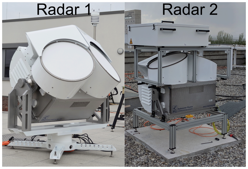
Figure 1 Impressions of the two frequency-modulated continuous wave (FMCW) W-band radars used in this study, as indicated in Table 2. Images courtesy of the radar owners.

Table 1 Some key technical specifications of the analyzed W-band radars.

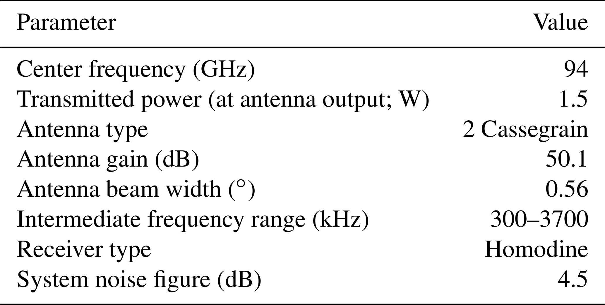
Table 2 Information of type, data periods, and calibration of the radars used for this study.

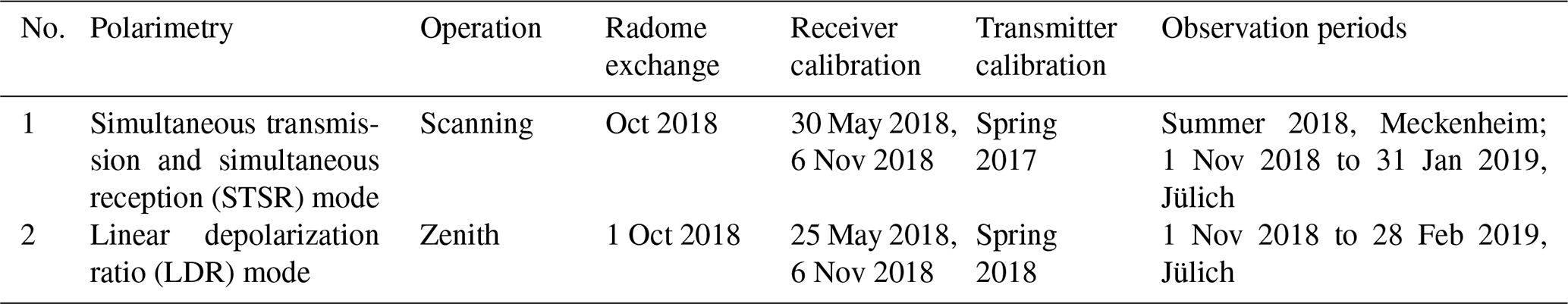
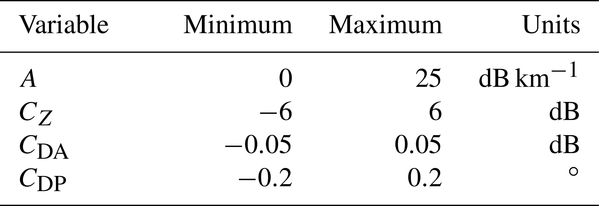
Table 3 Ranges of values for differential evolution (DE) used in the self-consistency method.

2.2 In situ instruments

The radars are equipped with Vaisala WXT520 weather stations (Basara et al., 2009) which provide atmospheric pressure, temperature, relative humidity, and a 1 min averaged rainfall rate derived from a piezoelectric sensor. The optical disdrometer PARSIVEL² (hereafter Parsivel; Löffler-Mang and Joss, 2000; Tokay et al., 2014) and the rain-weighing gauge PLUVIO² (denoted as Pluvio throughout the paper) are manufactured by OTT HydroMet GmbH, Kempten, Germany. They belong to the permanently installed instrumentation of JOYCE-CF (roof platform; 17 m above ground level). Due to a site maintenance, Parsivel and Pluvio were operated, until 27 November 2018, on a nearby roof at a ca. 50 m distance from the radars. From 27 November 2018 on, both instruments were reinstalled very close to the radars, with distances of less than 10 m. The Pluvio installed at JOYCE-CF has a 200 cm² orifice and a single Alter-type wind shield (precipitation wind shield; OTT HydroMet GmbH; Kochendorfer et al., 2017). Data are recorded with a 1 min averaging period; the real-time output product is used for this study. Parsivel is an optical disdrometer which uses a laser band to detect the size and fall velocity of precipitating particles (Löffler-Mang and Joss, 2000; Löffler-Mang and Blahak, 2001; Tokay et al., 2014). The Parsivel software groups the measured drop sizes and velocities into a predefined 32×32 matrix. The size and velocity bins can be found in Angulo-Martínez et al. (2018). Rain rate and reflectivity are calculated using the raw data (32×32 matrix). A similar optical disdrometer, namely the laser precipitation monitor (LPM; Fig. 2a) from Adolf Thies GmbH & Co. KG (Angulo-Martínez et al., 2018), has continuously been operated at the RPG site since 14 June 2018. The LPM collected data during summer 2018 at RPG site; from 1 November 2018 to 6 December 2018 the LPM was installed at the JOYCE-CF site as part of TRIPEX-pol campaign. The LPM provides a particle event mode in which a message with the size and velocity of each individual particle is generated (Prata de Moraes Frasson et al., 2011). The particle event mode is normally used for calibration purposes. The particle’s size and velocity is provided separately, assuming either a spherical or a “hamburger” shape. The latter shape lacks a detailed description in the LPM manual; hence, we decided to only use the values for the spherical shape. Prata de Moraes Frasson et al. (2011) report that the data transfer rate may not be sufficient for a large number of particles. The manufacturer also notes in the LPM manual that not all particles may be registered at high precipitation rates. Unfortunately, a more detailed explanation of this issue and whether it is related to the data transfer rate or to other well-known issues of optical disdrometers, such as multiple particles in the field of view or partial beam filling, is missing. We developed a test device to estimate the underestimation of events due to limited data transfer rate. A chopper wheel with two closed and two open quadrants was mounted to either completely block or open the LPM laser beam (Fig. 2b). The event frequency was registered with a photo transducer and subsequently increased in steps from 3.7 to 83.2 s⁻¹. The data from the LPM were transferred using a serial RS485 full duplex connection with 115 kBaud transfer rate. The LPM detected the event rate with an accuracy of 1 up to 77 s⁻¹. Larger event rates were significantly underestimated by the LPM. If we assume a Marshall–Palmer distribution, the event rate due to a rainfall rate of 20 mm h⁻¹ is 30 s⁻¹. As most rainfall events analyzed in this study are well below this rainfall rate, the LPM data transfer problem is unlikely to introduce large uncertainties. A more serious issue for rainfall measurements with the LPM is splashing effects which have been found by Angulo-Martínez et al. (2018) to cause up to a 20 % overestimation of the particle number. In order to reduce the splashing effects, we covered all the LPM surfaces with spongy and cotton material (Fig. 2a). In order to further reduce the effects of splashing on the calculated rain rate and reflectivity, we followed the approach of Tokay et al. (2014) and rejected all particles with velocities outside the range of ±50 % relative to a theoretical size–velocity relation (Foote and Du Toit, 1969).

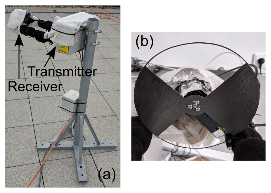
Figure 2 The laser precipitation monitor (LPM) at the Radiometer Physics GmbH (RPG) site (a). Metal surfaces close to the laser beam are covered with spongy and/or cotton material to mitigate splashing. The chopper wheel (b) was mounted on side of the LPM detector to test the data transmission rate (see text for details).

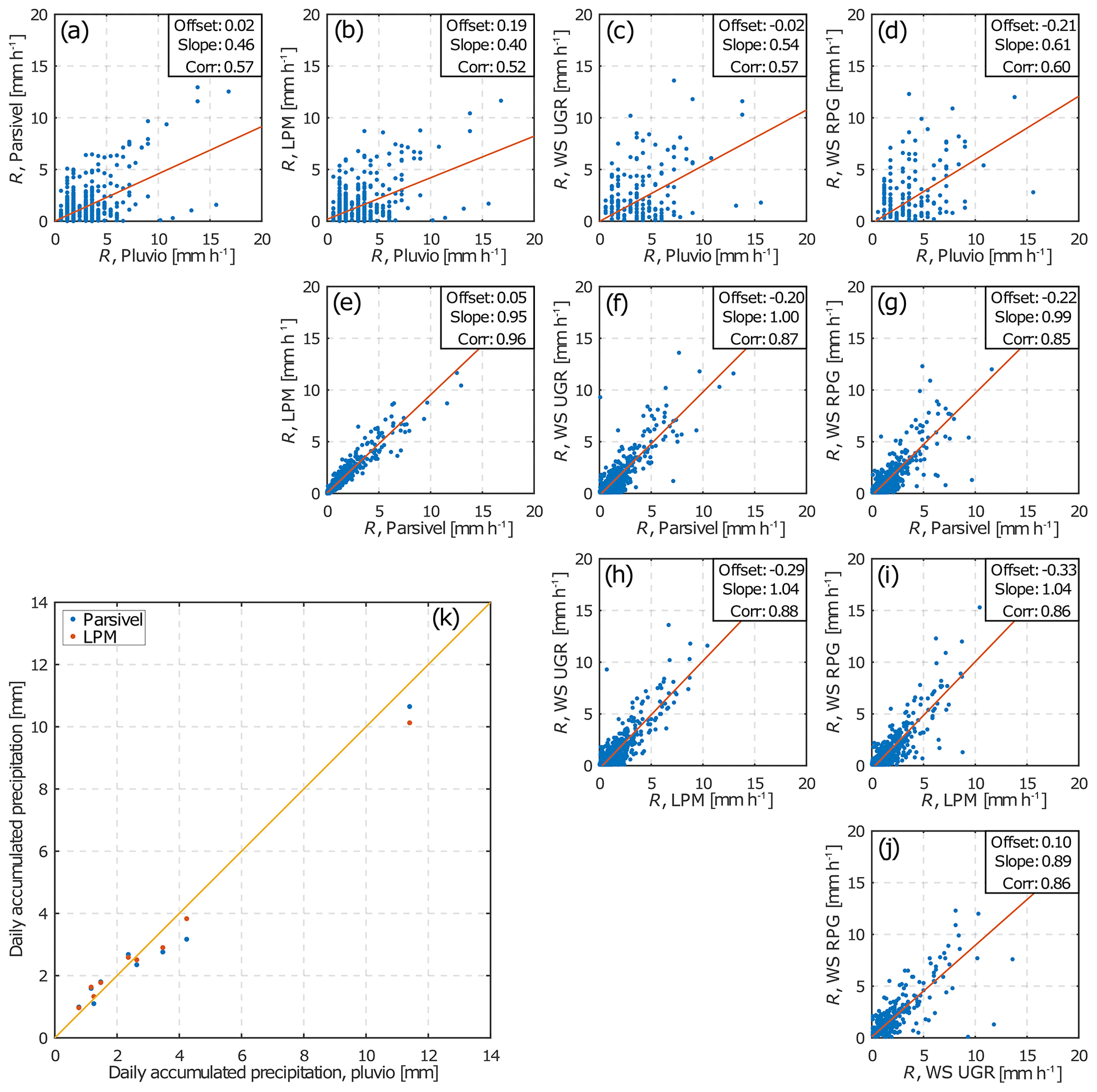
Figure 3 A comparison of 1 min rain rates observed by Pluvio, Parsivel, LPM, and the two Vaisala WXT520 weather stations attached to the radars (a–j). The weather stations of radars 1 and 2 are denoted as WS UGR and WS RPG, respectively. The data set from the TRIPEX-pol campaign (1 November 2018 to 6 December 2018) contains 391 min of rainfall detected by all sensors simultaneously. Each subplot contains the estimated offset and the slope of a linear fit (red line) and the Pearson correlation coefficient. Panel (k) shows a comparison of the daily accumulated precipitation from Pluvio, Parsivel, and LPM from 10 precipitating days. The yellow line is the one-to-one relation.

Figure 3 shows a comparison of the measured 1 min rain rates from the four in situ sensors. The basis for the comparison is observations from 1 November 2018 to 6 December 2018. In total, we found 391 min of precipitation detected by all sensors. The observed rain rates were mainly below 7 mm h⁻¹. The correlation between LPM and Parsivel rainfall rates is 0.96; LPM shows slightly smaller values than Parsivel. The two weather stations show a correlation with disdrometers varying from 0.84 to 0.88. These correlations are in an agreement with Prata de Moraes Frasson et al. (2011). The 1 min rainfall rates provided by Pluvio were found to be very noisy, with correlations to the other in situ sensors ranging from 0.5 to 0.6. Nevertheless, the 1 d accumulated precipitation from Pluvio correlates well with those from the Thies and Parsivel (0.997 and 0.99, respectively, calculated with 10 rainy days). As Pluvio is a weighting gauge, it measures the mass representing accumulation of droplets in the bucket. The rainfall rate is derived from the time derivative of accumulated mass, which can lead to more noisy rainfall rates. In contrast, optical disdrometers measure every single droplet crossing the laser beam and calculate the accumulated rainfall as an integral over time. The accumulated precipitation from Vaisala WXT520 weather stations has not been stored and, therefore, cannot be analyzed.

3 Method 1: the self-consistency method for W-band polarimetric cloud radars

Goddard et al. (1994) developed a calibration approach for 3 GHz radars based on observations of reflectivity Z, differential reflectivity Z_DR, and specific differential phase K_DP in rain at low elevation angles. At the S band, Z_DR defines the K_DP∕Z ratio because Z and K_DP depend on the number concentration of droplets, while Z_DR is a proxy for drop median size (Ryzhkov et al., 2005; Kumjian, 2013). For Z_DR exceeding 2 dB, which is often observed in strong rainfall, the relation between the three parameters is not affected by DSD variability. Z_DR and Z profiles can thus be used in strong rainfall to reconstruct the expected differential phase Φ_DP profile. The radar is considered to be well calibrated if the expected and the measured profiles of Φ_DP agree. According to Chandrasekar et al. (2015), a standard accuracy, which can be achieved for Z_DR, is about 0.1 dB. K_DP is calculated as a range derivative and, therefore, is immune to the radar polarimetric calibration. As a small bias in Z_DR affects the expected Φ_DP profiles much less than a bias in Z, any difference between measured and expected profiles of Φ_DP is assigned to a reflectivity offset. The reflectivity calibration factor is then simply determined by shifting the reflectivity profile until a minimum between the estimated and measured profiles of Φ_DP is reached.

Hogan et al. (2003) noticed that the method of Goddard et al. (1994) is not directly applicable to W-band radars for the following reasons. First, attenuation due to rain is almost negligible at 3 GHz, while it strongly increases towards higher frequencies. Second, non-Rayleigh scattering causes reflectivity at the W band to increase much less with the rainfall rate as compared to lower frequencies. As a result, W-band reflectivities become less sensitive to the rain rate with increasing rain intensities (Hogan et al., 2003). Third, in contrast to lower frequencies, Z_DR at the W band does not exceed 0.12 dB for rain rates up to 150 mm h⁻¹ (Aydin and Lure, 1991). Fourth, an estimation of K_DP from radar observations becomes more complicated. Otto and Russchenberg (2011) and Trömel et al. (2013) show that the total measured differential phase is the sum of a backscattering and a propagational component (see Eq. B6). At low frequencies, the backscattering differential phase δ is usually negligible, but it increases with larger frequencies. At millimeter wavelengths, even relatively small drops in the range of 2–3 mm diameter produce up to a 10^∘ backscattering differential phase (Matrosov et al., 1999). For a polarimetric calibration method applicable to millimeter wavelengths, it is thus crucial to find a way to separate δ and K_DP. In order to find a solution to the abovementioned problems, we identify a set of different propagation and backscattering variables to which an approach similar to Goddard et al. (1994) can be applied. To infer suitable relations between radar observables, we simulate them using the T-Matrix model (Mishchenko, 2000) and a range of particle size distributions (PSDs) similar to Hogan et al. (2003). We assume normalized gamma distributions with μ from 0 to 15 and N_L from 5×10² to 2.5×10⁴ mm⁻¹ m⁻³. For the given μ and N_L, the median volume diameter D₀ was increased in 0.05 mm steps, starting at 0.1 mm until the rain rate reached 20 mm h⁻¹. A detailed description of how the nonattenuated reflectivity Z₀, one-way attenuation A, differential reflectivity Z_DR, specific differential phase K_DP, differential attenuation A_DP, and backscattering differential phase δ are calculated can be found in Appendices A and B.

3.1 Replacement for Z_DR

As discussed above, Mie scattering effects complicate the use of Z_DR at the W band, and we need to find an alternative parameter which is closely related to D₀. Trömel et al. (2013) found, at the X band, that δ is a suitable parameter which is independent of N_L and sufficiently related to D₀. As can be seen in Fig. 4, δ is nearly directly proportional to D₀ at the W band for rain rates up to 7 mm h⁻¹, and even at larger rain rates, δ seems to be a reasonable proxy for D₀. Thus, we will use δ in the following as a replacement for Z_DR used at lower frequencies in order to find relations between Z₀ and propagation variables.

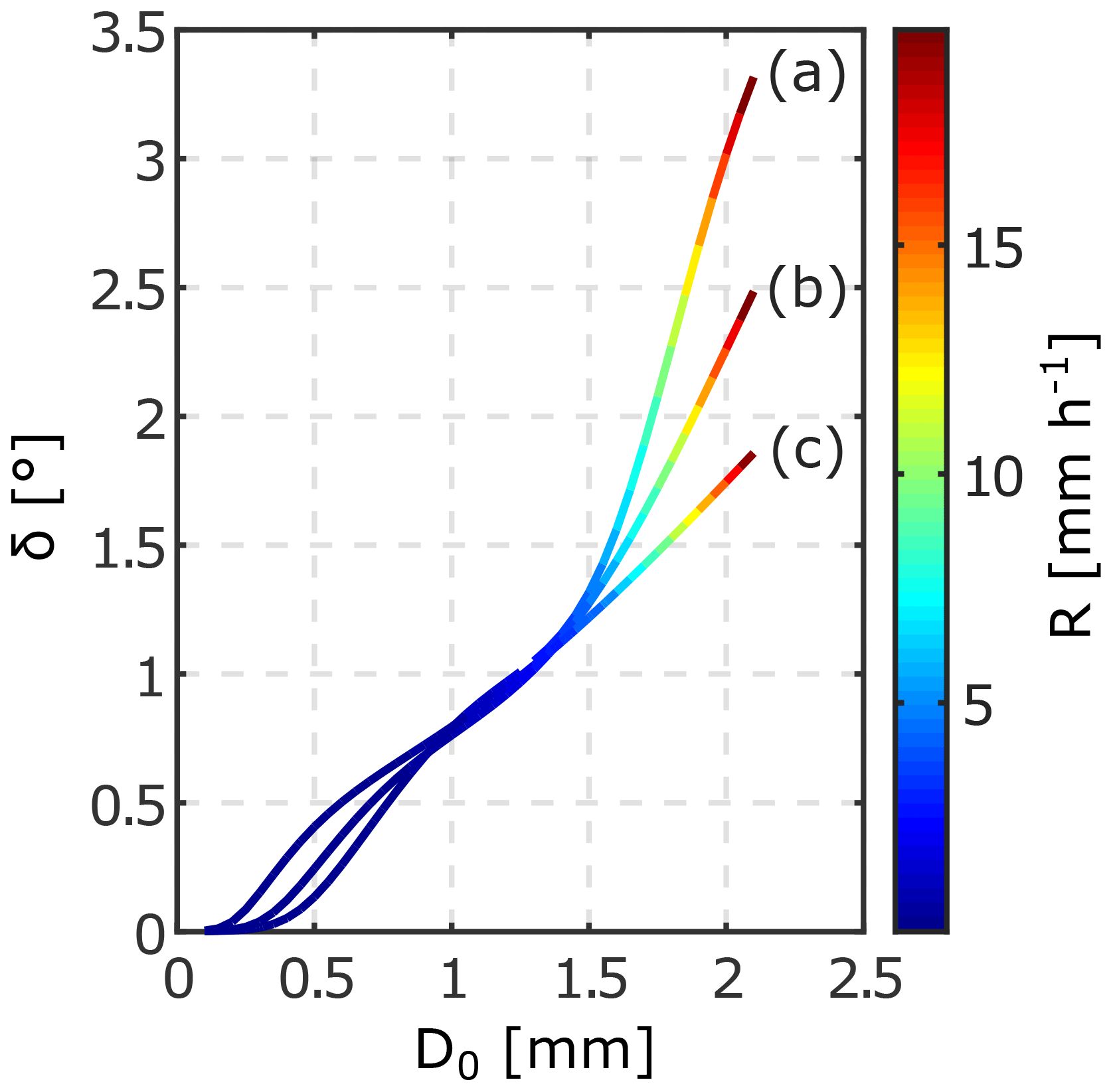
Figure 4 Simulated relations between the backscattering differential phase δ and the median drop diameter D₀ at 94 GHz. The curves show simulations for DSDs, with N_L=2500 mm⁻¹ m⁻³ and μ equal to 5 (a), 0 (b), and 15 (c). The corresponding rain rate R is color coded; the maximum rain rate for all simulations is limited to values smaller than 20 mm h⁻¹. The calculations are made for a 20 ^∘C and 30^∘ elevation angle.

3.2 Relations between propagation and backscattering variables

In the original method of Goddard et al. (1994), a ratio of the propagation parameter K_DP and the backscattering parameter Z₀ is parameterized as a function of Z_DR characterizing the median drop size. Using the large set of simulated rain PSDs introduced above and the corresponding forward-simulated radar parameters, we can parameterize the ratio K_DP∕Z₀ as a function of δ for the W band as follows:

$$\begin{array}{}\text{(1)}& \begin{array}{rl}{\displaystyle \frac{K_{\mathrm{DP}}}{Z_{\mathrm{0}}}}& =a_{\mathrm{1}}f(a_{\mathrm{2}}\mathit{\delta }+a_{\mathrm{3}})+a_{\mathrm{4}}f(a_{\mathrm{5}}\mathit{\delta }+a_{\mathrm{6}})\\ & +a_{\mathrm{7}}f(a_{\mathrm{8}}\mathit{\delta }+a_{\mathrm{9}})+a_{\mathrm{10}}.\end{array}\end{array}$$

At frequencies where rain attenuation is nonnegligible, we also need to parameterize specific attenuation A. The backscattering differential phase δ also defines the ratio A_DP∕A as follows:

$$\begin{array}{}\text{(2)}& \begin{array}{rl}{\displaystyle \frac{A_{\mathrm{DP}}}{A}}& =b_{\mathrm{1}}f(b_{\mathrm{2}}\mathit{\delta }+b_{\mathrm{3}})+b_{\mathrm{4}}f(b_{\mathrm{5}}\mathit{\delta }+b_{\mathrm{6}})\\ & +b_{\mathrm{7}}f(b_{\mathrm{8}}\mathit{\delta }+b_{\mathrm{9}})+b_{\mathrm{10}}.\end{array}\end{array}$$

We also introduce an additional relation to constrain relations between Z₀ and δ. This is done by coupling these two parameters via the absolute value of the specific attenuation A in dB km⁻¹ as follows:

$$\begin{array}{}\text{(3)}& \begin{array}{rl}A& =c_{\mathrm{1}}f(c_{\mathrm{2}}\mathit{\delta }+c_{\mathrm{3}}{Z}_{\mathrm{0}}+c_{\mathrm{4}})+c_{\mathrm{5}}f(c_{\mathrm{6}}\mathit{\delta }+c_{\mathrm{7}}{Z}_{\mathrm{0}}+c_{\mathrm{8}})\\ & +c_{\mathrm{9}}f(c_{\mathrm{10}}\mathit{\delta }+c_{\mathrm{11}}{Z}_{\mathrm{0}}+c_{\mathrm{12}})\\ & +c_{\mathrm{13}}f(c_{\mathrm{14}}\mathit{\delta }+c_{\mathrm{15}}{Z}_{\mathrm{0}}+c_{\mathrm{16}})+c_{\mathrm{17}}.\end{array}\end{array}$$

In Eqs. (1)–(3), f is the following function:

$$\begin{array}{}\text{(4)}& f\left(x\right)={\displaystyle \frac{\mathrm{2}}{\mathrm{1}+e^{-\mathrm{2}x}}}-\mathrm{1}.\end{array}$$

The approximations (Eqs. 1–3) were derived using the neural network approach. The used neural networks have one hidden layer with three neurons for Eqs. (1) and (2) and four neurons in Eq. (3). The neural networks were trained with the Levenberg–Marquardt backpropagation algorithm. This algorithm utilizes the advantages of the Gauss–Newton and the steepest descent methods. The Gauss–Newton algorithm converges fast if the current point is close enough to the optimum but is slow if it is far from the optimum. The deepest descent, in contrast, converges better if the current point is far from the optimum but has bad convergence in the area of the optimum. By combining these two approaches, the Levenberg–Marquardt algorithm, in general, converges faster. The problem of overfitting was avoided by using the low number of neurons in the hidden layer and applying the Bayesian regularization (MacKay, 1992), which restricts the magnitude of the weights. Further details and examples, with ready-to-use MATLAB codes of function approximations using neural networks, can be found in Demuth et al. (2014).

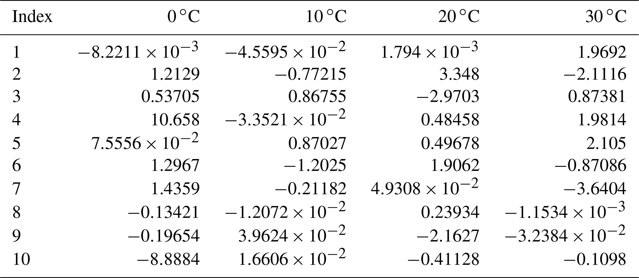
The fit coefficients a₁₋₁₀, b₁₋₁₀, and c₁₋₁₇ are given in Tables A1, A2, and A3, respectively. In Eqs. (1)–(3) the units of Z₀, A, K_DP, A_DP, and δ are mm⁶ m⁻³, dB km⁻¹, ^∘ km⁻¹, dB km⁻¹, and ^∘ respectively. In the Supplement, we provide MATLAB and Octave functions for Eqs. (1)–(3). In order to take into account the possible variability in Eqs. (1)–(3) caused by environment temperature, the fit coefficients are provided for 0, 10, 20, and 30 ^∘C.

Figure 5 shows the simulated polarimetric variables and the fitted approximations (Eqs. 1–3). The remaining root mean square error (RMSE) of the K_DP∕Z₀, A_DP∕A, and A approximations is $\mathrm{2.3}\times {\mathrm{10}}^{-\mathrm{4}}$ ^∘ ${\text{km}}^{-\mathrm{1}}{\text{m}}^{\mathrm{3}}{\text{mm}}^{-\mathrm{6}}$, $\mathrm{3.2}\times {\mathrm{10}}^{-\mathrm{4}}$ dB km⁻¹ dB⁻¹ km, and 0.3 dB km⁻¹, respectively. The correlations between the simulated variables and their approximations are 0.998. Figure 5a indicates that, at δ close to 0.5^∘, K_DP∕Z₀ is close to 0, which represents a limit of the self-consistency method. The method becomes robust at δ values exceeding 1^∘.

3.3 Separating propagational and backscattering components using Doppler spectra

Profiles of Z₀, A, δ, A_DP, and K_DP are not directly measured by a dual polarized cloud radar. Instead, the radar measures variables (Z, Z_DR, and Φ_DP) which are combinations of propagational and backscattering effects, as can be seen in Eqs. (A1), (B5) and (B6). Several studies presented approaches to separate propagational and backscattering components for centimeter wavelength radars (Otto and Russchenberg, 2011; Schneebeli and Berne, 2012; Trömel et al., 2013). These approaches are based on relations between profiles of Z_DR and δ (Otto and Russchenberg, 2011; Schneebeli and Berne, 2012) and A and K_DP (Trömel et al., 2013). However, as already discussed above, those methods cannot be applied to the W band because of non-Rayleigh scattering and attenuation effects. As a result, Z_DR becomes less informative, and relations between A and K_DP vary for different DSDs when δ exceeds 1^∘.

A common approach for separating backscattering from propagational effects is the use of Doppler spectra. In the absence of strong turbulence, smaller droplets populate in the slow-falling part of the spectrum, while the larger drops are found on the fast-falling side. Due to the relatively well-known relation of drop size and terminal velocity, the spectral power at each velocity bin can be associated to a certain drop size range (Kollias et al., 2002). The small droplets can be assumed to only be affected by propagational effects, while the larger drops are also affected by Mie scattering effects. Therefore, the spectral information can be used to separate the two components in low turbulence conditions. This approach has been applied to nonpolarimetric dual wavelength spectra in rainfall and snow to separate the attenuation and Mie scattering effects (Tridon and Battaglia, 2015; Tridon et al., 2017; Li and Moisseev, 2019). Here we follow the same idea but with polarimetric spectra.

Polarimetric Doppler spectra have only been sporadically used in the past, probably due to the demands regarding storage capacity and required high data quality. At centimeter wavelength, their potential has been shown for microphysical retrievals (Moisseev and Chandrasekar, 2007; Spek et al., 2008; Dufournet and Russchenberg, 2011; Pfitzenmaier et al., 2018) and efficient clutter suppression (Unal, 2009; Moisseev and Chandrasekar, 2009; Alku et al., 2015). The number of installed polarimetric Doppler cloud radars has only recently increased, with only a few studies, so far, exploring their potential for microphysical studies and retrievals (Oue et al., 2015, 2018; Myagkov et al., 2015, 2016b).

As shown by Aydin and Lure (1991), drops up to a size of 1.2 mm do not produce a strong backscattering differential reflectivity z_DR at the W band. At sizes larger than 1.2 mm, the z_DR spectrum reveals a series of minima and maxima. The authors also simulated a velocity z_DR spectrum for 1 mm h⁻¹. The values of z_DR are nearly 0 dB below 3 m s⁻¹ terminal velocity, and therefore, any changes in Z_DR in this terminal velocity range can be addressed to differential attenuation.

We therefore derive differential reflectivity from the Doppler velocity range 0–2 m s⁻¹, where we assume all particles to be Rayleigh scatterers (hereafter referred to as the small size part of a Doppler spectrum). Estimating this small particle Z_DR individually for each range bin directly provides us with the profile of the cumulative differential attenuation DA as follows:

$$\begin{array}{}\text{(5)}& \mathrm{DA}\left(r\right)=C_{\mathrm{DA}}-\mathrm{2}\underset{\mathrm{0}}{\overset{r}{\int }}{A}_{\mathrm{DP}}\left(r\right)\mathrm{d}r,\end{array}$$

where C_DA is an offset in differential reflectivity in dB due to the polarimetric calibration. Uncertainties of the DA profile can be characterized using the variances of Z_DR over the small size part of the spectra. Unfortunately, Aydin and Lure (1991) do not show the size spectrum of δ. Nevertheless, as it is shown for lower frequencies (Matrosov et al., 1999; Ryzhkov, 2001; Trömel et al., 2013), and as we further show in Sect. 3.6, the spectrally resolved δ shows a similar oscillatory behavior to z_DR. Applying the same approach as described above, we can estimate the cumulative differential phase DP from the Φ_DP in the small size part of the spectrum as follows:

$$\begin{array}{}\text{(6)}& \mathrm{DP}\left(r\right)=C_{\mathrm{DP}}+\mathrm{2}\underset{\mathrm{0}}{\overset{r}{\int }}{K}_{\mathrm{DP}}\left(r\right)\mathrm{d}r,\end{array}$$

where C_DP is an offset in differential phase in degrees due to the polarimetric calibration. The profile of δ can simply be estimated by subtracting DP from the Φ_DP profile (see Eq. B6).

Spectral polarimetric observations are typically performed at low elevation angles (≤45^∘; Unal and Moisseev, 2004; Spek et al., 2008) in order to maximize the polarimetric signatures of hydrometeors. Doppler velocities corresponding to each spectral bin represent projections of terminal velocities of drops, vertical air motions, and horizontal wind. In order to separate propagation and backscattering effects, the knowledge of the absolute terminal velocities is not required. The effect of air motions (both vertical and horizontal) can be roughly mitigated by shifting spectra in such a way that the rightmost detected spectral line, corresponding to drops with the slowest fall velocity, is set to 0 m s⁻¹. As it is shown in Sect. 3.6, such a rough mitigation is good enough to separate small drops scattering in the Rayleigh regime from those producing resonance effects.

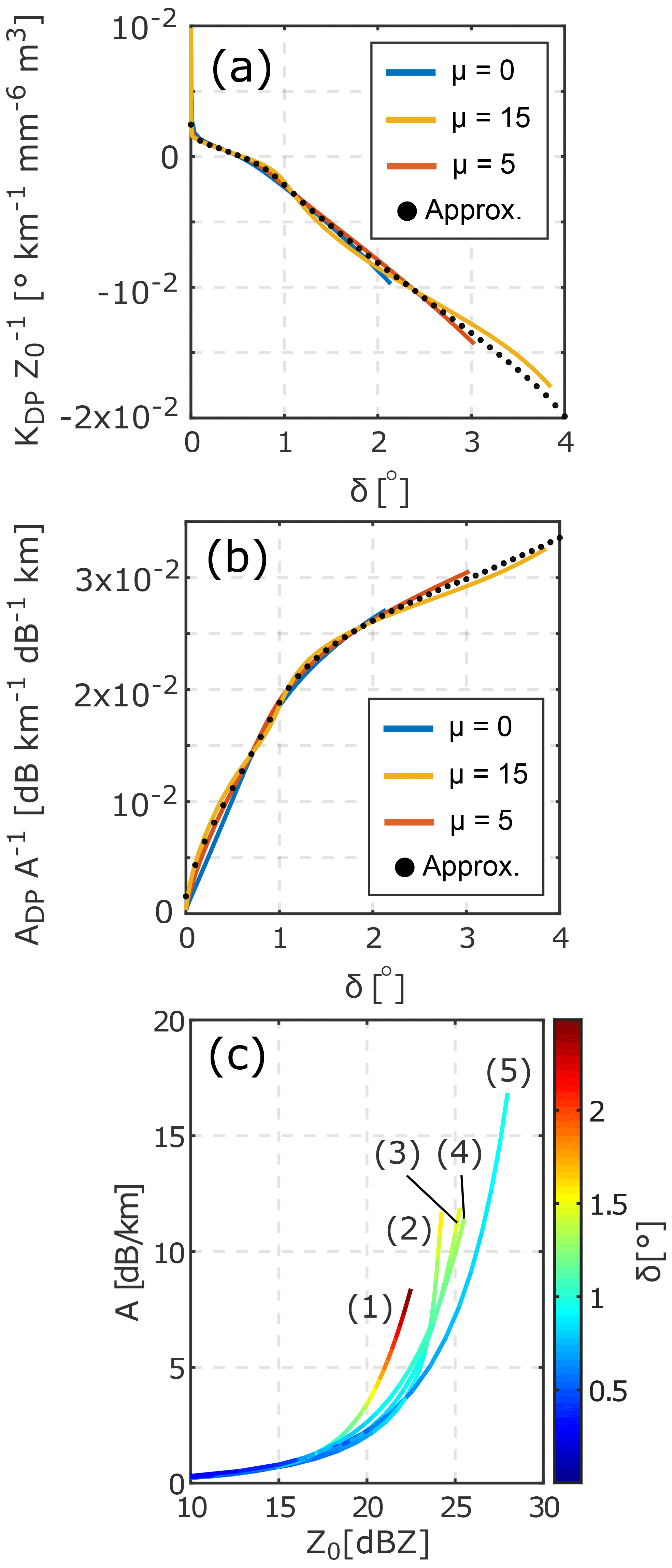
Figure 5 Relations between K_DP, Z₀, and δ (a), A_DP, A, and δ (b), and A, Z₀, and δ (c) at 94 GHz. The solid lines show the calculations for different DSDs, and the black dots denote the fitted approximations (Eqs. 1a and 2b). In panel (c), the calculations are made for μ=5 and N_L=2500 mm⁻¹ m⁻³ (1), μ=15 and N_L=8000 mm⁻¹ m⁻³ (2), μ=5 and N_L=8000 mm⁻¹ m⁻³ (3), μ=0 and N_L=8000 mm⁻¹ m⁻³ (4), and μ=5 and N_L=25000 mm⁻¹ m⁻³ (5). The rain rates are all smaller than 20 mm h⁻¹. All calculations are made for a 30^∘ elevation angle and a temperature of 20 ^∘C. The units of Z₀, A, K_DP, and A_DP in panels (a) and (b) are mm⁶ m⁻³, dB km⁻¹, ^∘ km⁻¹, and dB km⁻¹, respectively.

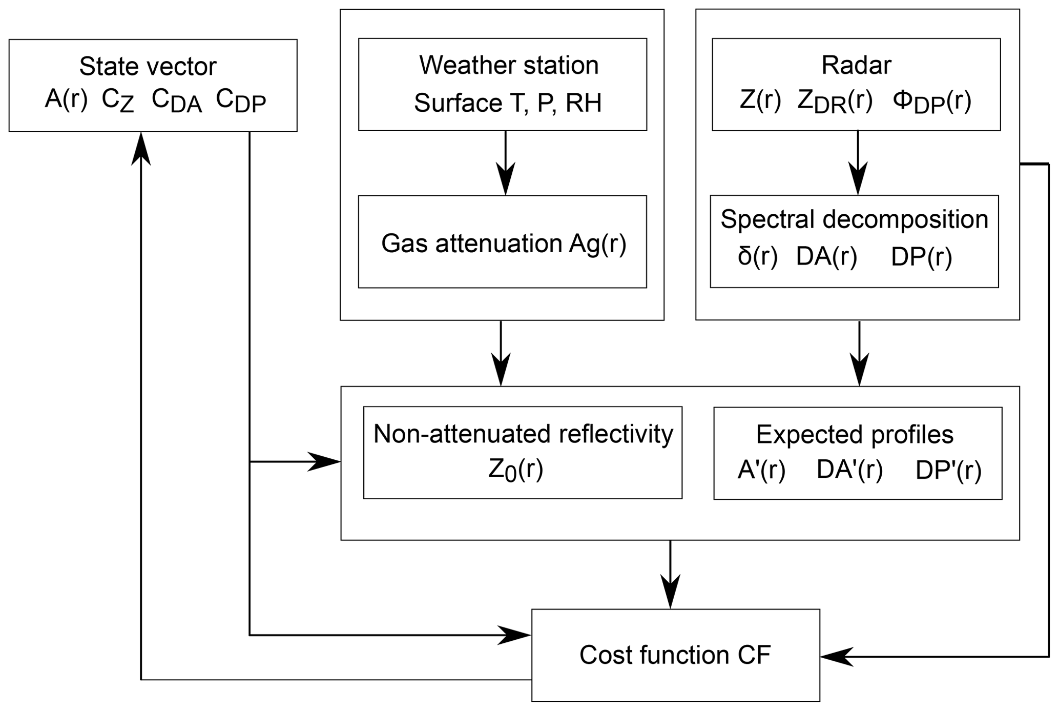
Figure 6 Schematic illustrating the processing steps of the self-consistency method. A detailed description can be found in the text.

3.4 Algorithm

The different modules of the method are illustrated in Fig. 6. The method is based on finding a state vector corresponding to an optimal match of the expected and the observed radar variables. The matching is achieved by minimizing a cost function using a global stochastic optimization method called the differential evolution (DE) approach (Storn and Price, 1997). DE was recently used by Rusli et al. (2017) for a detailed characterization of drizzle and cloud liquid. In this study, we use the built-in Octave implementation of DE, which is based on Das et al. (2009). We use the default strategy DEGL/SAW/bin with a mutation factor of 0.8, a crossover probability of 0.9, a tolerance of 10⁻³, a maximum number of iterations of 200, and a population size of NP=20 N_v, where N_v is the number of elements in the state vector. DE stops when the maximum number of iterations is reached or the relative difference in the cost function between the best and the worst state vector in the population is below the specified tolerance. When DE reaches one of the stopping criteria, the state vector with the lowest cost function is taken as the output.

The state vector contains a range profile of A(r) (dB km⁻¹) and the calibration factors of C_Z (dB), C_DA (dB), and C_DP (^∘). DE does not require an a priori state vector. Instead, it requires realistic limits for each element of the state vector (Table 3). Within each iteration, the DE algorithm stochastically creates NP state vectors.

From each generated state vector, a profile of Z₀ is calculated as follows:

$$\begin{array}{}\text{(7)}& \begin{array}{rl}{Z}_{\mathrm{0}}\left(r\right)& =Z\left(r\right)+C_Z+\mathrm{2}\underset{\mathrm{0}}{\overset{r}{\int }}\left[A\left(r\right)+A_{\mathrm{g}}\left(r\right)\right]\mathrm{d}r\\ & -\mathrm{10}{\log }_{\mathrm{10}}|K_{\mathrm{0}}{|}^{\mathrm{2}}+\mathrm{10}{\log }_{\mathrm{10}}|K{|}^{\mathrm{2}},\end{array}\end{array}$$

where Z(r) is the measured reflectivity profile in dBZ, and $|K_{\mathrm{0}}{|}^{\mathrm{2}}$ is the dielectric factor assumed in the radar software (0.74 for our radars). The two dielectric factors in Eq. (7) account for the differences in the actual dielectric properties of liquid water and those assumed in the radar software. Surface observations of temperature, relative humidity, and pressure are used to estimate the attenuation profile due to gases A_g(r) (see Sect. A2). The dielectric factor $|K{|}^{\mathrm{2}}$ is calculated for liquid water at surface temperature. Using profiles of Z₀ and δ, an expected profile DP^′ is found using Eq. (1). The prime is used to discriminate the expected variable from the one estimated from measurements. Profiles of A and δ are used to estimate the expected DA^′ profile from Eq. (2). Finally, the expected profile of A^′ is calculated using the expected profiles of DA^′ and DP^′ and Eq. (3).

The profiles of A^′, DA^′, and DP^′ are further used for the calculation of the cost function, CF, as follows:

$$\begin{array}{}\text{(8)}& \mathrm{CF}={\mathrm{CF}}_{\mathrm{DA}}+{\mathrm{CF}}_{\mathrm{DP}}+{\mathrm{CF}}_A,\end{array}$$

where

$$\begin{array}{}\text{(9)}& {\mathrm{CF}}_i={\left[{\mathit{w}}_i-{\mathit{W}}_i\right]}^T{\mathbf{S}}_i^{-\mathrm{1}}\left[{\mathit{w}}_i-{\mathit{W}}_i\right].\end{array}$$

In Eq. (9), i specifies a variable and w_i contains the profile of the expected values for the ith variable (DA, DP, and A). The vector W_i contains the profile of the ith variable inferred from measurements. The attenuation profile in the current state vector is taken as W_A. S_i is the error covariance matrix of the ith variable. Nondiagonal elements of S_i are assumed to be 0 since no correlation between errors in different range bins is expected. Based on uncertainty estimates of A (see Sect. 3.2) related to uncertainties in the approximation Eq. (3), diagonal elements of S_A are set to (0.3 dB km⁻¹)². Estimation of DA and DP from radar observations and their diagonal elements in the error covariance matrix is done as described in Sect. 3.3.

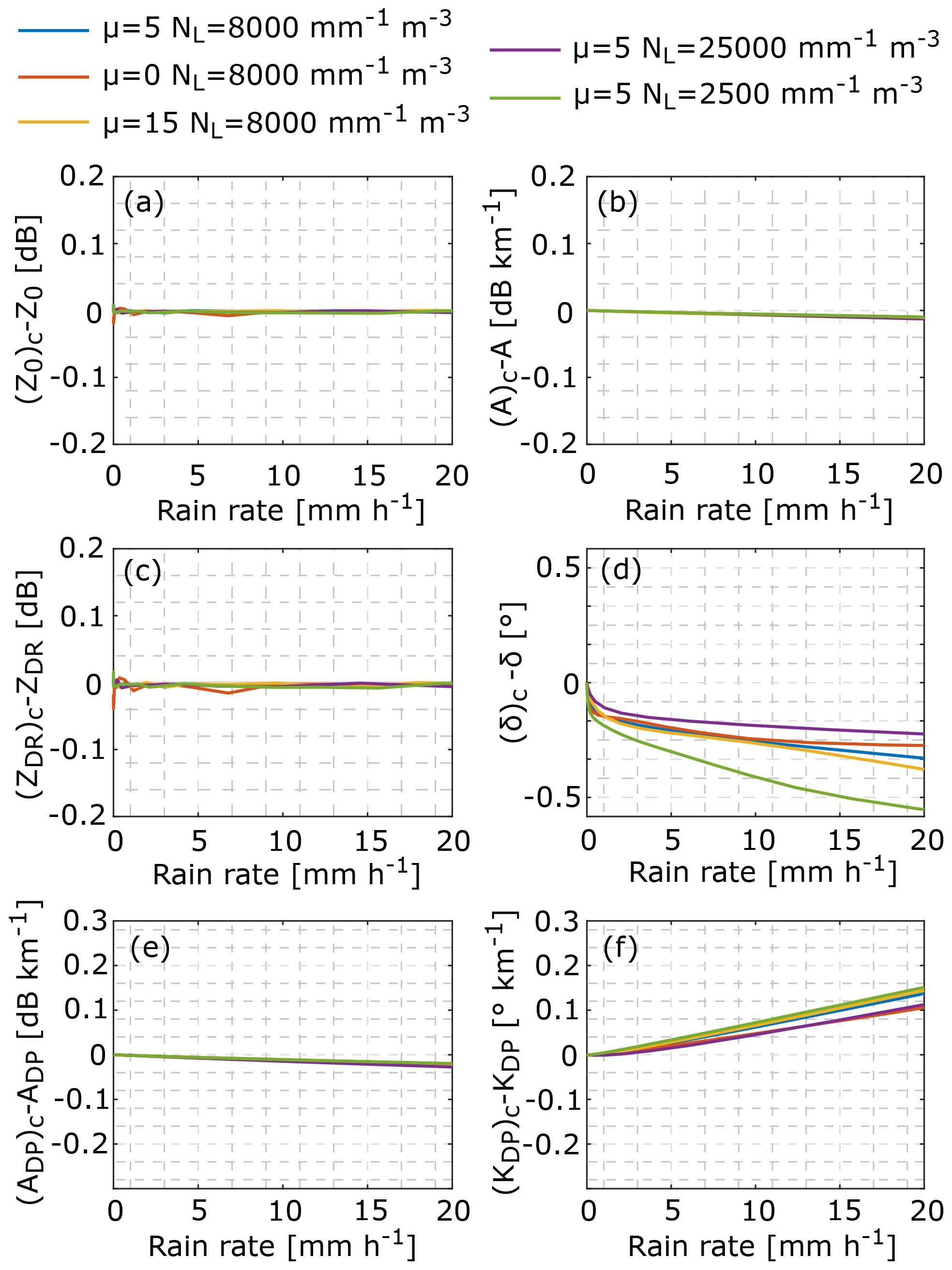
Figure 7 Differences between reflectivity (a), specific attenuation (b), differential reflectivity (c), backscattering differential phase (d), differential attenuation (e), and specific differential phase (f) calculated with a 10 and 0^∘ standard deviation of the canting angle distribution. Variables calculated with 10^∘ are indicated by the index “c”. The differences are shown for different DSDs and are indicated by line colors.

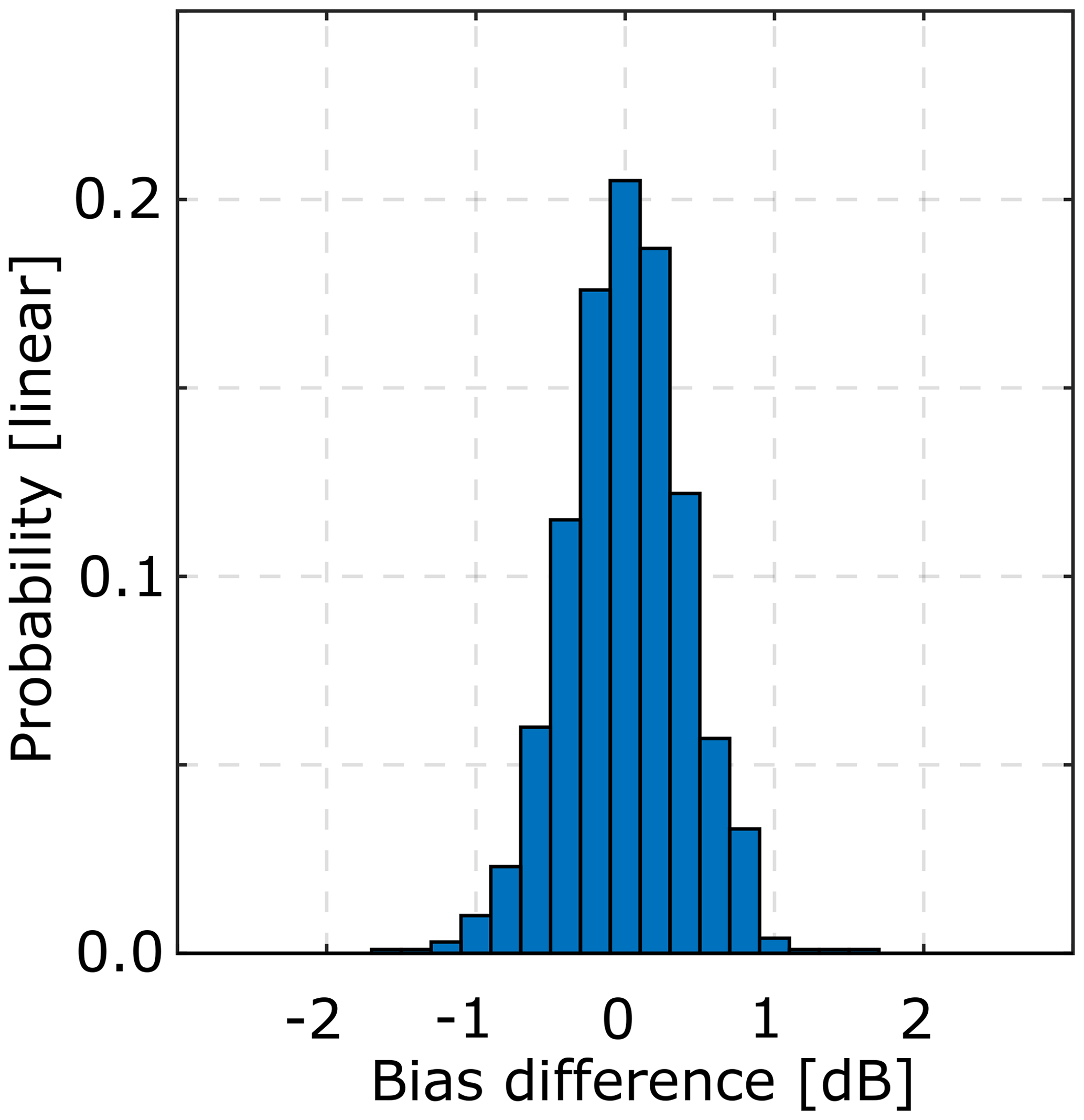
Figure 8 Estimated uncertainty of the reflectivity calibration coefficient C_Z using the self-consistency method (Sect. 3). Various rain DSDs were used to simulate ideal profiles of radar variables. Random noise was then added to these profiles and several calibration coefficients before applying the self-consistency method (also see details in the text). The distribution shows the difference between original C_Z and the retrieved value. The 5th and 95th percentiles and the standard deviation of the distribution are −0.7, 0.7, and 0.4 dB, respectively.

3.5 Uncertainties of the method

In order to estimate the uncertainties of the method, we simulated 1000 samples of slanted 1 km profiles of Z₀, A, A_DP, K_DP, and δ, as described in Appendices A and B. For the simulations, the normalized gamma DSD were used with μ and N_L, randomly chosen for each sample and each range bin. The ranges of μ and N_L were from 0 to 15 and from 5×10² to 2.5×10⁴ mm⁻¹ m⁻³, respectively. Size distributions with A less than 3 dB km⁻¹ were excluded from the analysis because such attenuation values are close to the magnitude of the measurement variability. In order to take into account the measurement variability of radar reflectivity, a random Gaussian noise was added to Z₀ with variance set to $Z_{\mathrm{0}}^{\mathrm{2}}/\mathrm{20}$, where 20 is the typical number of spectra averaged by the used radars (Eq. 5.193 in Bringi and Chandrasekar, 2001). Taking into account that the signal-to-noise ratio in rain within the first kilometer typically exceeds 30 dB and the copolar correlation coefficient in rain approaches one, variability in the polarimetric variables is low (Sect. 6.5 in Bringi and Chandrasekar, 2001) and is thus neglected. With the simulated variables, the profiles of Z, DA, and DP were derived. Variability in the calibration constants of C_Z, C_DA, and C_DP were randomly generated, assuming the uniform distributions given in Table 3, and added to Z, DA, and DP, respectively. The uncertainties in C_Z, C_DA, and C_DP are assumed to be the same for all range bins for a single sample.

The forward model of the radar observables used in this study assumes that raindrops are oriented horizontally. A number of studies show that drops typically have a canting angle distribution with zero mean and a standard deviation up to 10^∘ (Bringi and Chandrasekar, 2001; Huang et al., 2008). In order to check the level of uncertainty introduced by the drop orientation, we compared simulated radar variables with a 0 and 10^∘ standard deviation of the canting angle distribution. The sensitivity experiment was made for a 0^∘ elevation, when the strongest effect of the canting angle on polarimetric variables is expected. The canting angle is assumed to be in the polarization plane. The results shown in Fig. 7 indicate that the canting angle mainly affects the backscattering and specific differential phase. The uncertainties become larger with the rain rate due to the larger number of large oblate drops included. At 20 mm h⁻¹ the uncertainties might reach ∼0.5^∘ and 0.2^∘ km⁻¹ in the backscattering and specific differential phase, respectively. Uncertainties in the other variables are negligibly low. In order to take into account the uncertainties related to the canting angle distribution and also the separation of δ and DP, we added a random Gaussian noise with a standard deviation of 0.5^∘ to DP and subtracted the corresponding values from δ. Similarly, a random Gaussian noise with a standard deviation of 0.3 dB was added to DA. All noise values were different for each range bin and each sample. As it will be shown in Sect. 3.6, standard deviations of DP and DA measured for a single spectral line corresponding to the Rayleigh scatterers are typically about 0.3^∘ and 0.3 dB, respectively. An averaging over spectral lines, from 0 to 2 m s⁻¹, would reduce the standard deviations by a factor of 3–4. Thus, the assumed uncertainties of 0.5^∘ and 0.3 dB are conservative and exceed the actual measurement uncertainties.

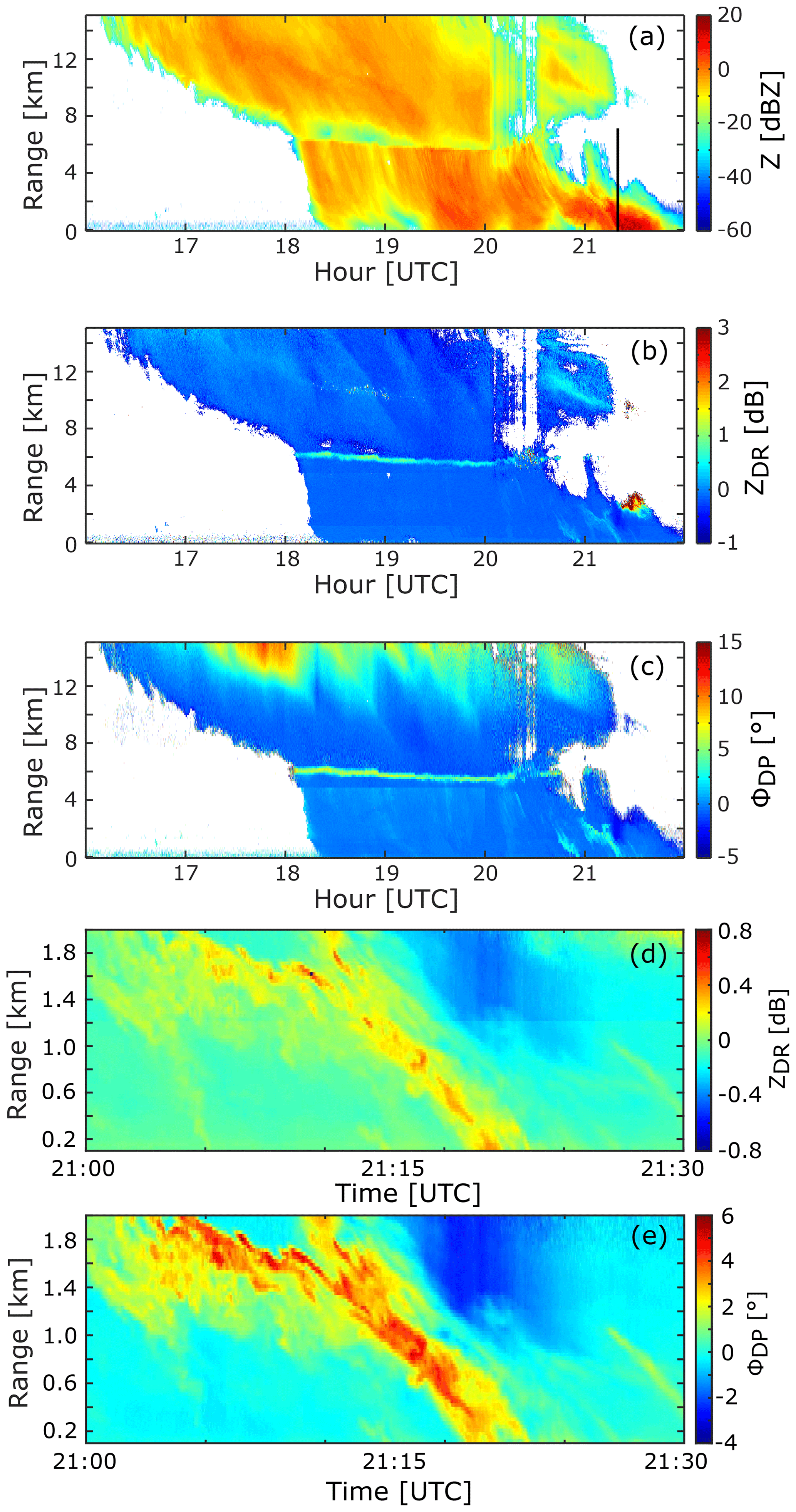
Figure 9 Time range cross sections of radar reflectivity (a), differential reflectivity (b), and differential phase (c). Panels (d) and (e) are an enlarged view of the differential reflectivity and differential phase, respectively. The observations were taken by the radar 1 on 9 June 2018 in Meckenheim, Germany. The radar was pointed to a 30^∘ elevation. The range corresponds to the slanted distance from the radar. The black vertical line in (a) indicates the time sample used for the spectral analysis shown in Fig. 10.

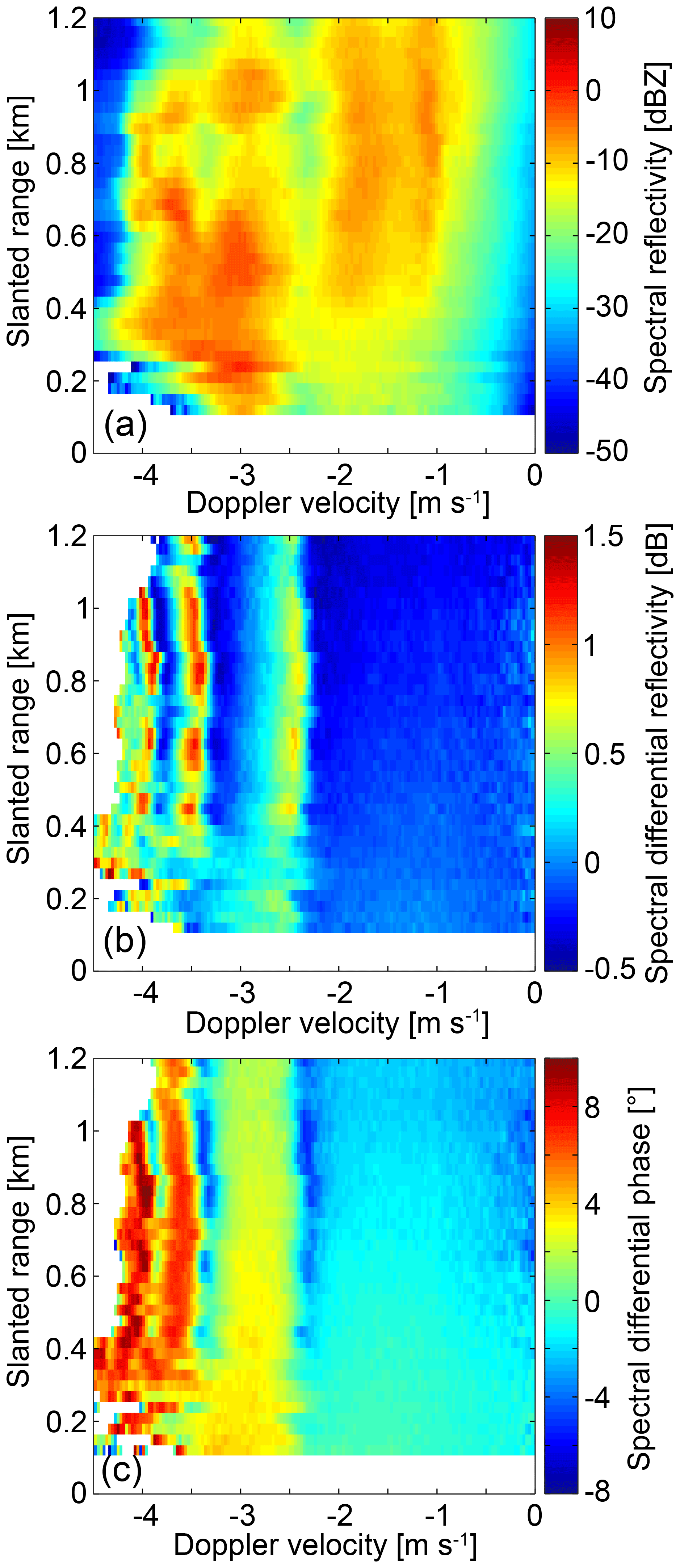
Figure 10 Range profiles of Doppler spectra of reflectivity (a), differential reflectivity (b), and differential phase (c). The measurements were taken by radar 1 on 9 June 2018 at 21:19:23 Coordinated Universal Time (UTC) in Meckenheim, Germany. The radar was pointed to a 30^∘ elevation. Negative velocities indicate movements towards the radar. Relatively slow (small) drops are on the right side of the spectrum profile, while the fast-falling (big) drops are on the left side. Note that, in order to make the figure easier to interpret, the horizontal wind contribution has been roughly mitigated by shifting the rightmost detected spectral line of a spectrum to 0 m s⁻¹.

The method was tested using the simulated profiles of Z, DA, and DP as input. For each sample, the best estimate of C_Z provided by the algorithm was then compared to C_Z used for the simulation. The results shown in Fig. 8 show that 90 % of the differences are within ±0.7 dB.

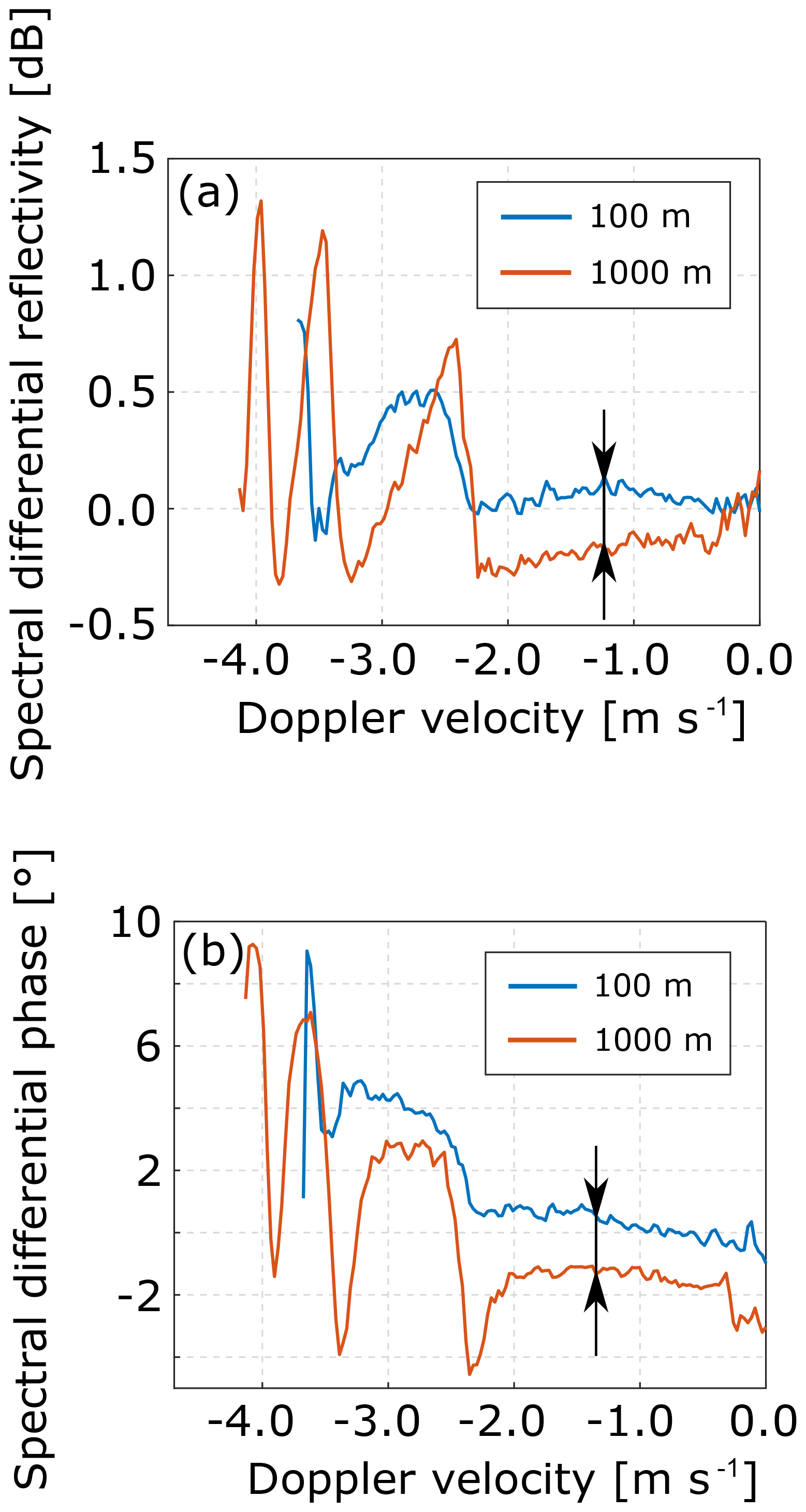
Figure 11 Doppler spectra of differential reflectivity (a) and differential phase (b) taken at 0.1 (blue lines) and 1 km (red lines) for the case shown in Fig. 10. The differences between the observations in the area of relatively slow-moving particles, indicated by the arrows, are associated with the propagation effects, namely differential attenuation in (a) and propagation differential phase in (b).

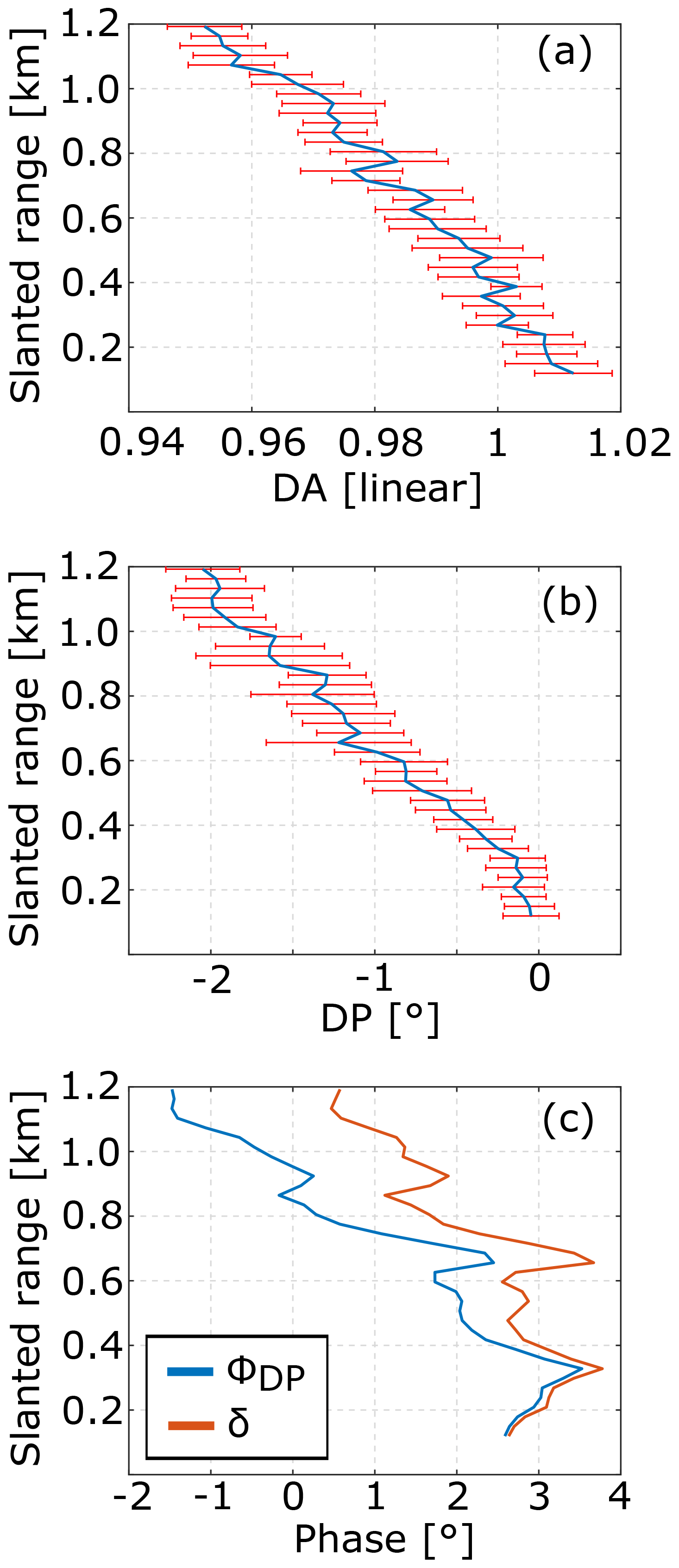
Figure 12 Profiles of differential attenuation or DA (a) and differential phase or DP (b), which are solely due to propagational effects. The profiles have been derived using the spectral decomposition technique, illustrated in Fig. 11, applied to the profiles of spectra shown in Fig. 10. Blue lines and red bars indicate mean values and ±1 standard deviation, respectively. Panel (c) shows the profiles of the differential phase Φ_DP (blue) and δ (red).

3.6 Application to measurements from radar 1

We now exemplarily demonstrate the different steps of the self-consistency method with a case study. A precipitation event, which includes drizzle and stronger rainfall, was observed at Meckenheim on 9 June 2018, operating the radar at a 30^∘ elevation (Fig. 9). The melting layer can be depicted at the height of 2.5 km by enhanced values of Z_DR and Φ_DP. During the period between 18:00 and 21:00 UTC the rain sensor only registered drizzle on the ground, while later a short and more intense rainfall event with up to 15 mm h⁻¹ rainfall took place. As expected, Z_DR and Φ_DP are close to zero in the drizzle part due to the near-spherical shape of the drops. Nonzero values are found during the stronger rainfall event due to the larger and, hence, more aspherical raindrops. Around 21:00 UTC positive and negative values in both Z_DR and Φ_DP are visible. These values indicate presence of backscattering and the propagational effects of raindrops.

Backscattering and propagational effects can be better separated when moving to the Doppler spectral space (Fig. 10). The spectra during the stronger rainfall event show the expected oscillatory behavior for larger Doppler velocities which are principally related to larger sizes. It should be noted that we only applied a very rough correction for horizontal wind as the method itself is not dependent on such a correction. The main goal in the spectral analysis is the separation of the Rayleigh scattering part (only affected by propagational effects) from the Mie scattering part (affected by both backscattering and propagational effects). The spectral part which is not affected by oscillations (approximately Doppler velocities slower than −2 m s⁻¹) shows decreasing values for Z_DR and Φ_DP, with an increasing range caused by propagational effects (see also spectra plotted for constant ranges in Fig. 11). The reflectivity spectra themselves show a somewhat unexpected increase in range, and also, the oscillations are less pronounced than in the polarimetric variables. This can be explained by the fact that Z is also dependent on the particle concentration.

The spectral regions with oscillatory behavior represent drop sizes for which backscattering and propagational effects are convolved (Fig. 11). In the part where the smaller droplets scatter in the Rayleigh regime, we find a plateau-like region in the spectra of Z_DR and Φ_DP (Fig. 11). The deviation of the plateau from 0 dB indicates the propagational effects. It should be noted that calibration offsets would, of course, also result in a shifted plateau region; however, this is independent of range. Z_DR and Φ_DP of radar 1 have been calibrated using zenith observations in light rain, as described in Myagkov et al. (2016a). Vertical observations in light rain show Z_DR and Φ_DP values of 1.003±0.01 (linear units) and $\mathrm{0}\pm \mathrm{0.15}{}^{\circ }$. After proper calibration, we can assign the shift of the plateau region solely to the propagation effects for which we derive mean and standard deviation for each range (Fig. 12). A_DP and K_DP are found, for this case, to be, on average, about 0.13 dB km⁻¹ and −0.95^∘ km⁻¹, respectively.

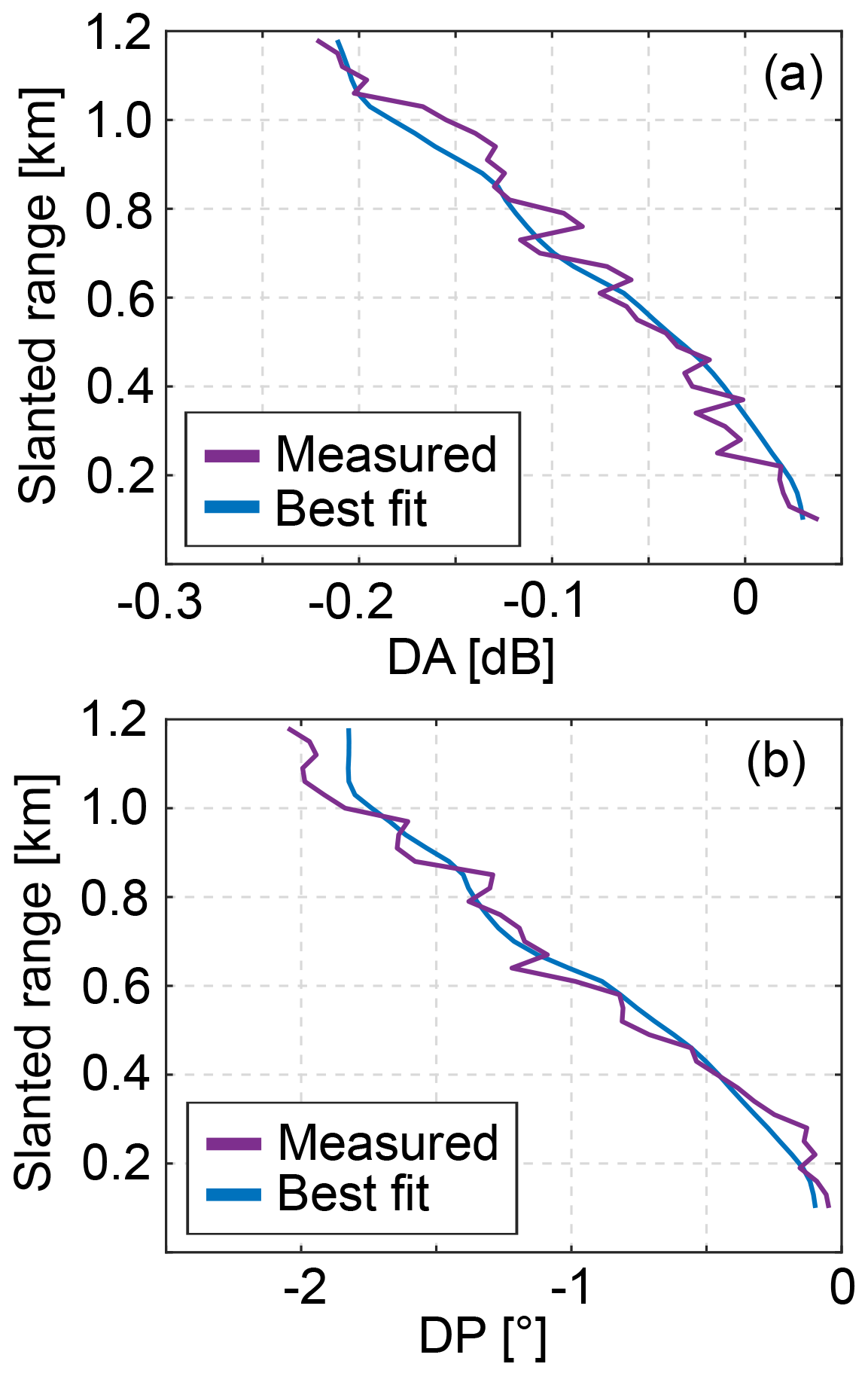
Figure 13 Range profiles of DA (a) and DP (b). Blue solid lines correspond to the best fit found by the self-consistency method for radar 1, with $C_Z=-\mathrm{0.7}$ dB. The magenta lines represent profiles estimated from the measurements (shown by blue lines in Fig. 12). The results are obtained for the cases shown in Figs. 10 and 12.

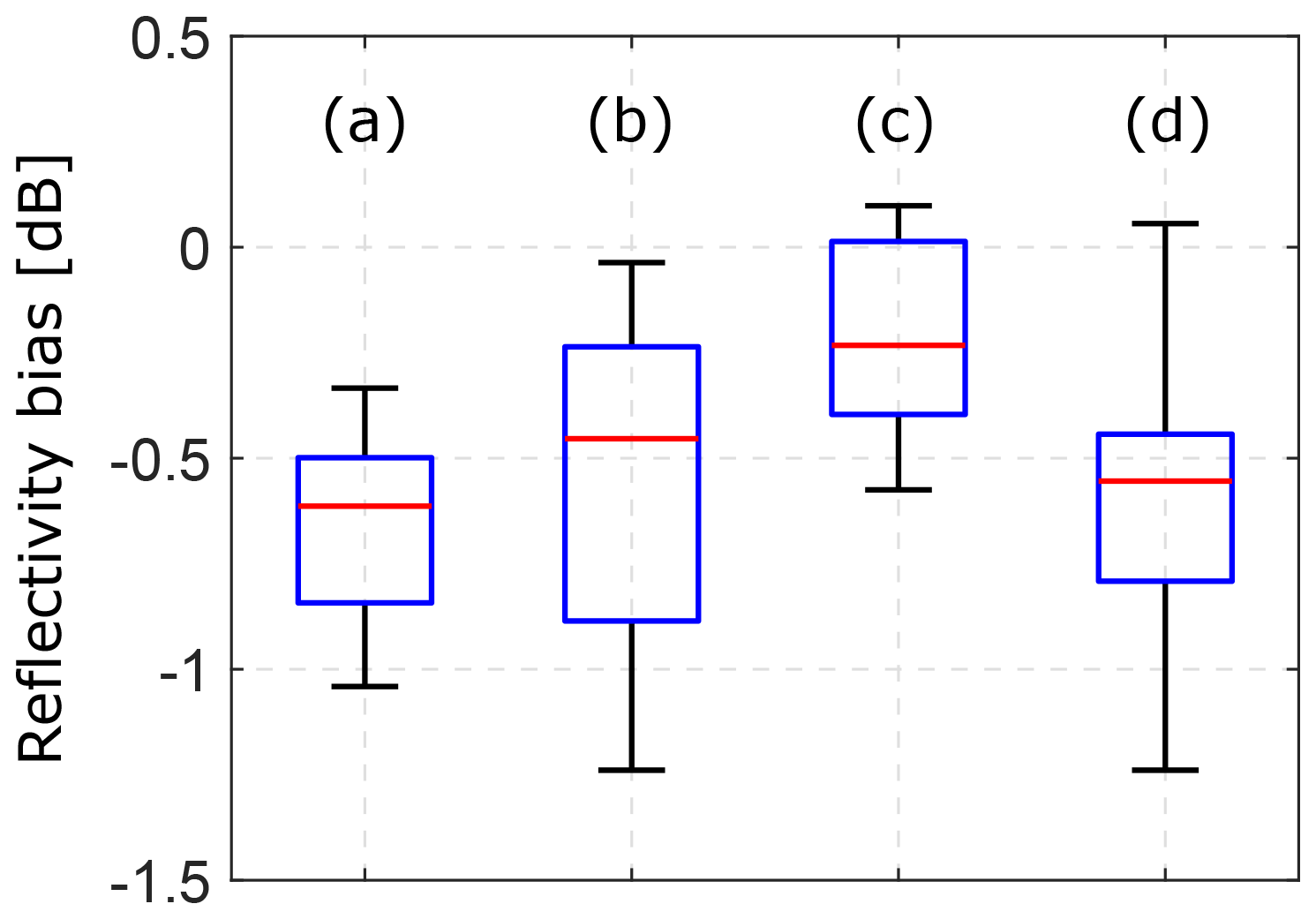
Figure 14 Reflectivity biases, due to the calibration coefficient C_Z, estimated using the self-consistency method applied to observations at a 30^∘ elevation angle during rain events on 9 June 2018 at 21:00 UTC (a), 20 July 2018 at 17:00 UTC (b), and 28 July 2018 at 11:22 UTC (c). The box plot (d) shows the results for all 64 available samples. The measurements were taken with radar 1 at the RPG site. The total number of samples are 45 for (a), 11 for (b), and 8 for (c). The upper and lower edges of the boxes correspond to the 75th and 25th percentiles, respectively. The upper and lower whiskers indicate the 95th and 5th percentiles, respectively. The horizontal red bars correspond to the median values.

In order to estimate a profile of δ, which is used as an input for Eqs. (1) and (2), the profile of DP, shown in Fig. 12b, is subtracted from the profile of Φ_DP. Profiles of Φ_DP and δ are shown in Fig. 12c.

Figure 13a–b show the best fits for DA and DP profiles found by the optimization algorithm. The resulting best matching radar calibration coefficient for reflectivity C_Z has been found for this time sample to be −0.7 dB, meaning that radar 1 slightly underestimates the reflectivity values.

The self-consistency method allows for an evaluation of the radar calibration even from a single sample. In order to test how repeatable the results of the self-consistency method are, we applied the method to 64 samples from three rain events. As shown in previous sections, the self-consistency method relies on propagation variables K_DP and A_DP, which are used to constrain profiles of Z. If the magnitudes of K_DP and A_DP are comparable with measurement noise, the method shows larger uncertainties. Using the approach described in Sect. 3.5, we identified the applicability range of the method. In order for the method to produce reasonable results, the rainfall events and associated profiles have to fulfill the following criteria: (1) rain rate observed at the surface by the weather station must be below 20 mm h⁻¹, (2) δ has to be larger than 1^∘ over at least a 900 m one-way range, (3) the median K_DP must be lower than –0.3 ^∘ km⁻¹, and (4) the median A_DP must be higher than −0.06 dB km⁻¹. The results shown in Fig. 14 indicate that radar 1 has a small negative reflectivity bias. The mean C_Z estimated from the 64 samples is −0.6 dB. The single sample estimate of C_Z from the three rain events varies from −1 to 0 dB, which is within the uncertainty of the method estimated in Sect. 3.5. One might see an increasing trend in C_Z, but taking into account the method uncertainty of ±0.7 dB and the few cases, the trend is not statistically significant. As will be shown further in the next section, a certain variability in C_Z can be explained by imperfections in the removal of liquid water from the radome.

The 30^∘ elevation used in this study was chosen, considering the following aspects: (1) the maximum Doppler resolution is obtained with zenith-pointing observations because the projection of the terminal velocity on the radar line of sight is the largest. However, at zenith the required polarimetric variables are close to zero. In the other extreme, (2) at a 0^∘ elevation, polarimetric signatures are the strongest, but the projection of the terminal velocity on the radar beam is close to zero. Thus, a 30^∘ elevation appears to be a good compromise for spectral polarimetry applications, but a detailed numerical study, which tries to identify the optimal elevation angle for this method, was not performed.

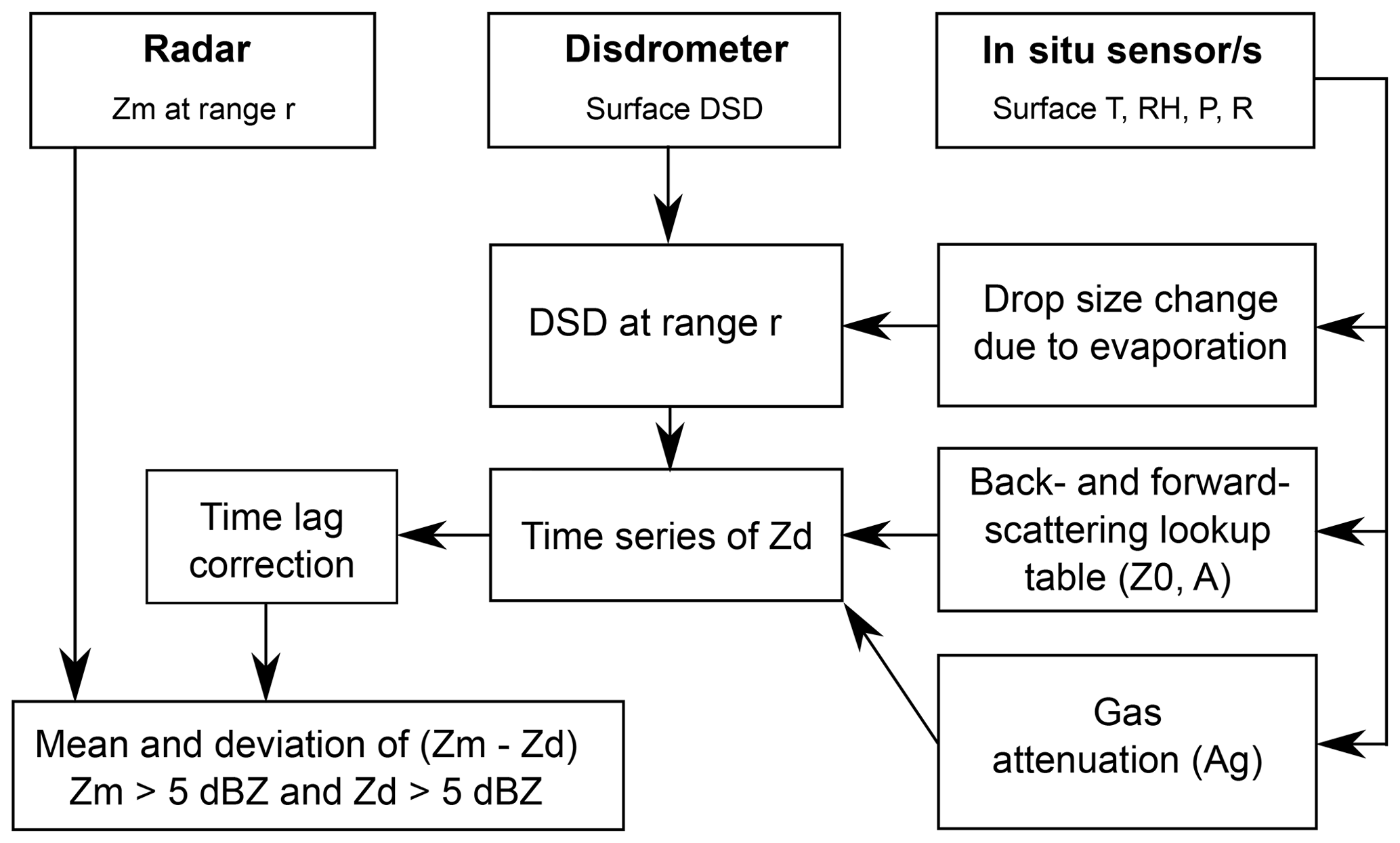
Figure 15 Schematic illustration of the extended disdrometer-based method. Detailed descriptions can be found in the text.

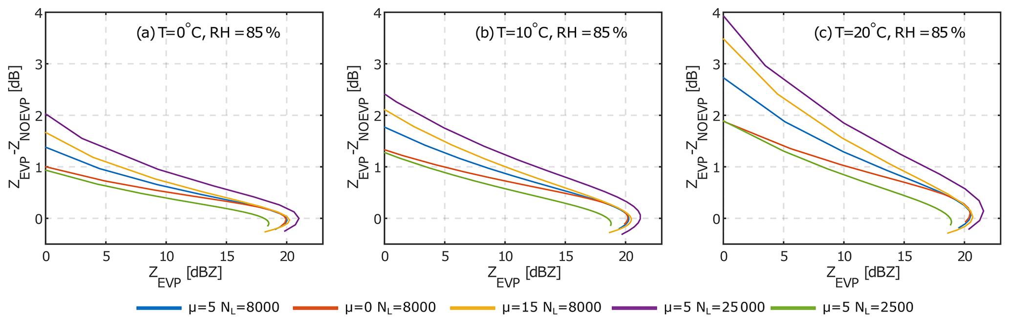
Figure 16 Simulated impact of evaporation on the simulated reflectivity at a 250 m range for DSDs measured at the surface. Z_NOEVP is the reflectivity at a 250 m range calculated with DSDs assumed at the surface, without taking evaporation into account. Z_EVP is the reflectivity at a 250 m range assumed for the same surface rain DSDs but corrected for drop evaporation within the 250 m layer. For the shown evaporation scenario, surface temperature and humidity are assumed to be 10 ^∘C and 85 %, respectively. The colors denote simulations with different rain DSD parameters. The effect of bending at Z_EVP values around 20 dBZ results from a faster increase in attenuation, with a rain rate relative to nonattenuated reflectivity (Hogan et al., 2003).

4 Method 2: disdrometer-based method

The second method is based on a comparison of the measured reflectivities (denoted as Z_m) at distances close to the surface with calculated reflectivities based on DSDs observed by colocated disdrometer (Z_d hereafter). Values of Z_d are calculated according to Appendix A. This well-known approach is generally applicable to radars operating at any frequency; however, the issue of variable rain properties between the lowest range gate and the disdrometer location remains a source of uncertainty. Using radar observations at the lowest range gates also requires that there are no antenna near the field or receiver saturation effects and that wet radome or wet antenna effects are minimized. For a two-antenna system, such as that used for the FMCW systems in this study, the incomplete beam overlap is corrected for using the method in Sekelsky and Clothiaux (2002). At ranges larger than 250 m from the radar, the beam overlap for all radars used is better than 90 %. For the following analysis, we use Z_m at a 250 m range. It should be noted that the calculations in this section use altitude and not range; for the slanted path, a conversion of range to altitude has to be applied. In the following, we will describe our approach for mitigating the two main sources of uncertainty for this method in the rainfall cases analyzed. A schematic of the entire processing chain is illustrated in Fig. 15.

4.1 Mitigating the effect of rain evaporation

Evaporation of rain on its way towards the surface is often observed at our sites. Figure 16 shows a simulation of the impact of evaporation on the reflectivity at 250 m. It can be seen that in subsaturated conditions the difference in radar reflectivity caused by evaporation can be strong. The effect is particularly pronounced for light precipitation, where the difference can exceed 2 dB. In this case, the scattering is dominated by relatively small drops whose diameters decrease faster due to evaporation than for big drops. In order to mitigate the effect of evaporation, we use an evaporation model described in Appendix A3. Based on temperature, relative humidity, and drop size at surface level, the model predicts the corresponding drop size at 250 m altitude.

For the calculations of drop sizes at a 250 m altitude, all drops detected by the LPM within 1 min prior to a radar sample time are used. In the case of Parsivel, which typically has a time resolution of 1 min, the data closest to a radar sample time are taken. The LPM in the single event mode provides diameters of single particles, and the evaporation model (Eq. A6) is directly applied to all detected drops. For Parsivel data, the evaporation model is applied to mean bin sizes, and the number of particles per size bin is assumed to be constant with altitude. Note that, in this case, the width of the size bin changes with altitude. This is equivalent to keeping the 32×32 raw data matrix – which is the standard output of Parsivel – constant but changing the mean drop diameters assigned to each matrix cell.

The estimated DSD for 250 m are then used for the calculation of Z₀ and A at 250 m, according to Table A5. Since the calculation of the whole attenuation profile with the evaporation effect accounted for is time consuming, A(r) is assumed to be constant and equal to the mean of A values at the surface and at 250 m taken in dB km⁻¹.

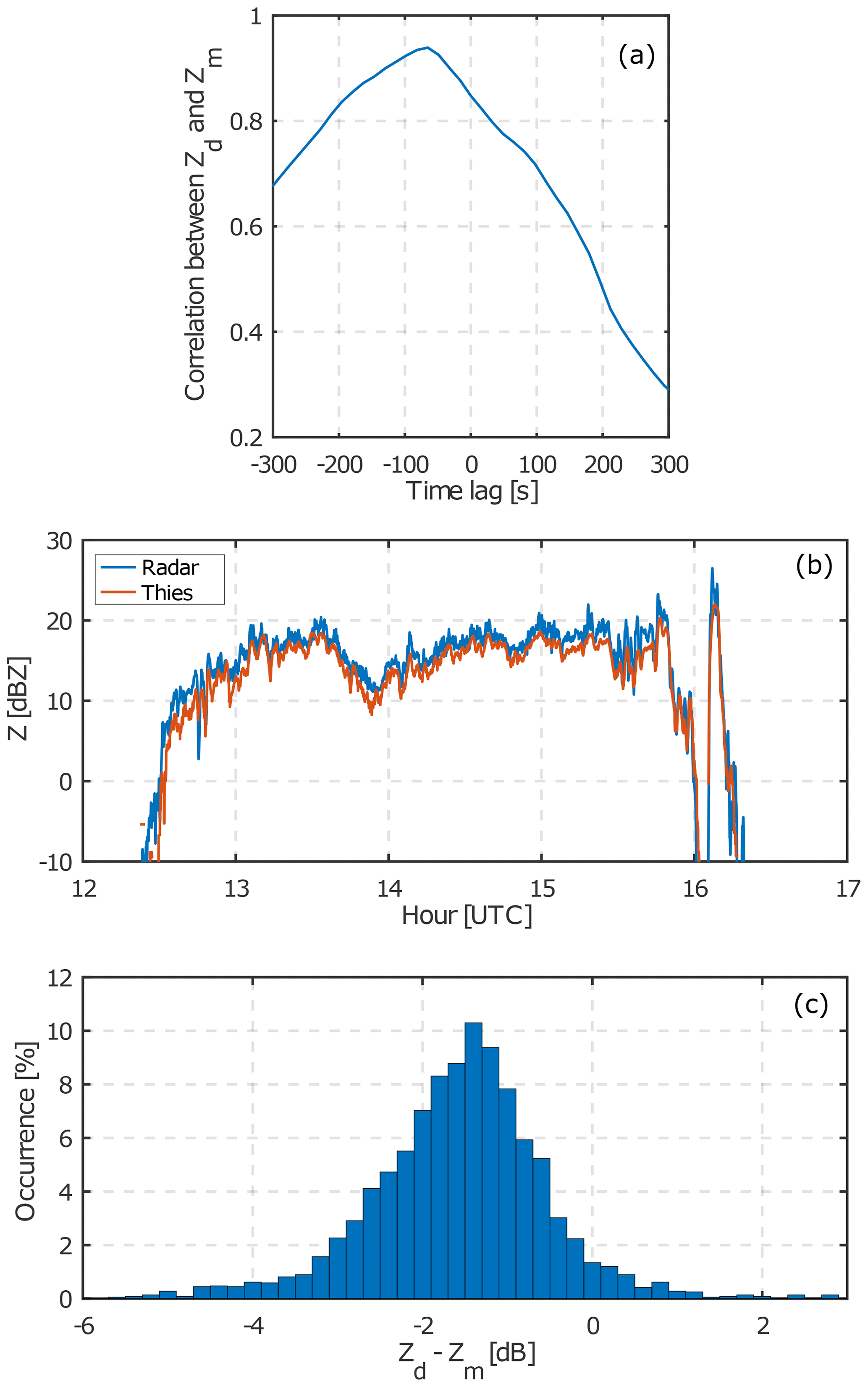
Figure 17 Correlation (a) between Z_d and Z_m at a 250 m distance from the radar for the rain event on 1 November 2018, observed by radar 2. Various time lags are successively applied in order to detect the most likely time delay (maximum correlation) between a 250 m range and surface level. Time series (b) of the reflectivity Z_m measured by radar 2 at 250 m altitude (blue line), and the reflectivity Z_d modeled from the LPM observations (red line). Panel (c) shows the distribution of Z_d−Z_m. Only 3 s samples for which Z_d and Z_m exceed 5 dBZ are used. The mean reflectivity difference is $-\mathrm{1.2}\pm \mathrm{0.3}$ dB. The standard deviation of the mean is calculated according to Appendix C.

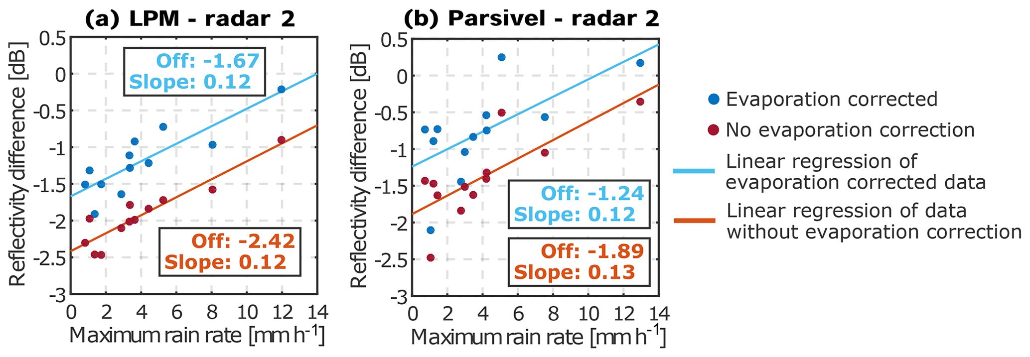
Figure 18 The results of the disdrometer-based method from 12 rain events. The calibration evaluation is made for radar 2 using LPM (a) and Parsivel (b). Each dot represents a result for a single rain event. Solid lines show linear regressions. Offsets and slopes of the regressions are given in the corresponding boxes. The colors of the dots and lines indicate whether the evaporation correction has been applied (blue) or not (red).

4.2 Comparison of expected and measured reflectivity time series

In order to identify a potential time lag between Z_m and Z_d, we calculate their temporal correlation assuming a range of time shifts. The time lag for which the maximum correlation is found is used for correcting the time series, and the difference between Z_m and Z_d is analyzed. We recommend only using Z_m and Z_d larger than 5 dBZ because the number of drops sampled by the disdrometer might be too low and not representative for smaller reflectivities.

4.3 Case study

We apply the disdrometer-based method to observations of radar 2 from 1 November 2018. From 12:30 to 16:20 UTC there was light precipitation at the JOYCE-CF site. The mean precipitation rate was 0.5 mm h⁻¹, with a maximum at 4.4 mm h⁻¹. The LPM operated in the particle event mode (see Sect. 2.2). Z_d are calculated according to Table A5. To calculate Z_d, all drop sizes have been corrected for evaporation. Figure. 17a shows the correlations between Z_d and Z_m at different time lags. The time shift corresponding to the maximum correlation of 0.93 is −65 s, which is applied to Z_d. After correcting for the time lag, Z_m and Z_d show a high correlation for values exceeding 5 dBZ (Fig. 17b). A direct comparison of Z_m and Z_d (Figs. 17c) shows that the mean difference in Z_d−Z_m is −1.2 dBZ, with a standard deviation of 0.3 dBZ (calculated according to Appendix. C).

4.4 Repeatability

In order to check how repeatable the results of the disdrometer-based method are, it was applied to LPM, Parsivel, and radar 2 observations in 12 rain events collected during the TRIPEX-pol campaign from 1 November 2018 to 6 December 2018. The same rain events are shown in Fig. 3. In the Supplement, we provide figures similar to Fig. 17 and statistical analysis for each rain event.

Figure 18 shows the reflectivity differences Z_d−Z_m for radar 2. The blue dots were calculated according to Sect. 4.1, while red dots were calculated without taking evaporation into account. Evaporation leads, on average, to about a 0.7 dB underestimation in Z_d, which might be critical if a reflectivity accuracy within ±1 dB is desired.

In Fig. 18 the differences in Z_d−Z_m are shown as functions of maximum rain rate observed by the disdrometers. At rain rates lower than 4 mm h⁻¹, values of Z_d−Z_m vary from −2 to −0.9 dB and from −2.1 to −0.5 dB, with mean values of −1.4 and −1.1 dB based on LPM and Parsivel (blue dots in Fig. 18a and c), respectively. On average, reflectivity values based on Parsivel observations are about 0.3 dB larger than those from LPM. The reason for this difference is likely related to the specific differences in the disdrometers; however, a detailed analysis of such differences is beyond the scope of this study. A comprehensive comparison of LPM and Parsivel disdrometers can be found, for example, in Angulo-Martínez et al. (2018) and Johannsen et al. (2020).

The results for both disdrometers indicate a dependence of the calibration offset on maximum rain rate observed during a precipitation event. Since the slope of the linear regressions is similar with and without the evaporation correction, we conclude that this effect may come from limitations in the rain mitigation system. However, the radome attenuation effects would certainly be much larger without a mitigation system. As shown by Hogan et al. (2003), those effects can easily exceed 10 dB for strong rainfall.

4.5 Comparison with the self-consistency method

As has been shown in the previous section, the comparison of radar 2 observations with LPM and Parsivel shows that the radar, on average, overestimates the reflectivity by 1.4 and 1.1 dB, respectively. The calibration of radar 1 was estimated using the self-consistency methods and indicates that the radar underestimates the reflectivity by 0.7 dB.

During the TRIPEX-pol campaign, radar 1 and radar 2 were operating at the JOYCE-CF site. Radar 1 was performing range–height indicator (RHI) and plan-position indicator (PPI) scans. As mentioned in Sect. 4.5, the disdrometer-based method does not often show consistent results when applied to scanning data. Nevertheless, radar 1 performed a PPI scan at a 85^∘ elevation every 15 min. Therefore, we used vertical observations from radar 2 and the PPI scans from radar 1 to find a reflectivity difference between radars 1 and 2. The difference can be used to check the consistency of the two calibration evaluation methods. During the 12 rain events we identified more than 8000 samples for the comparison. For each sample of radar 1, a closest time sample of radar 2 was found. Within each sample, we identified the closest range bins with reflectivity values exceeding 5 dBZ. Radar 2 shows, on average, 2.1 dB higher reflectivity values in comparison to radar 1. This value is consistent with the difference of 2.0±1.3 dB between the biases found by the two methods separately for radars 1 and 2.

5 Summary

Monitoring and evaluation of radar reflectivity calibration is a key requirement in order to provide long-term observational radar data sets to the cloud and precipitation community. In this study, we describe and compare two methods requiring very different degrees of complexity in terms of instrumentation and retrieval technique. Both methods use natural stratiform rainfall as the reference target.

The first method is an extension of the widely used approach from Goddard et al. (1994) applied to precipitation radars. The original method uses the $Z_{\mathrm{DR}}-K_{\mathrm{DP}}-Z$ relation, but due to the more complex attenuation and scattering behavior, this method is not directly applicable to millimeter wavelengths. In this study, we provide a solution for this problem using spectral polarimetry obtained from a W-band radar. The use of the spectral information allows us to disentangle propagational and backscattering effects. The method requires observations of Z_DR and Φ_DP and is only applicable to slanted observations in rain with distinct backscattering and propagational polarimetric signatures. The backscattering differential phase should mostly exceed 1^∘. The differential attenuation and specific differential phase should preferably be higher than 0.06 dB km⁻¹ and lower than −0.3^∘ km⁻¹, respectively. The main advantage of this method is its low sensitivity to variabilities in rain DSD. We estimated the uncertainty of this method based on realistic assumptions of errors in the profiles of radar observables to be within ±0.7 dB.

We also tested and extended a much simpler and more commonly used method, which compares reflectivities based on disdrometer DSDs measured at the surface with radar reflectivity at a close range gate. We included corrections for the time lag between the surface and elevated observations and a correction for evaporation. The method allows for a repeatable evaluation of the radar reflectivity calibration within ±0.9 dB, even with only a few hours of observations in rain with intensity below 4 mm h⁻¹. Averaging over a larger number of rain events allows us to further reduce the uncertainties of the method. The disdrometer-based method was tested with two common disdrometers of the LPM and Parsivel type. The results do not differ by more than 0.4 dB.

The two methods were used to evaluate the reflectivity calibration of two W-band radars. The self-consistency method showed that radar 1 underestimates the reflectivity by about 0.7±0.7 dB, while the disdrometer-based method indicated that radar 2 overestimates the reflectivity by 0.5–2.1 dB. Unfortunately, the rainfall rates during the parallel operation of the two radars at JOYCE-CF were not strong enough to compare the two methods directly. However, in case both methods provide reliable estimates for each radar, the reflectivity difference seen by both radars should be close to the sum of both offsets. Indeed, the observed reflectivity difference is, with 2.1 dB, quite consistent with the difference of 2.0±1.3 dB between the biases found separately by the two methods for radars 1 and 2. The derived calibration factors can be used to monitor the radar stability and to correct the observed reflectivity values, although we would also like to emphasize that a further evaluation of the two methods described here with other methods, e.g., using point target calibration or multi-frequency approach (Tridon et al., 2017) would be beneficial.

As wet radomes of W-band radar can cause attenuation exceeding 10 dB, the evaluation methods rely on efficient rain mitigation. We have found evidence that the reflectivity bias of the used radars is correlated to the maximum rain rate, and the slope of the linear regression is about 0.15 dB mm h⁻¹. The uncertainty of the used rain mitigation method is much smaller than the uncertainties and wet antenna effects reported by (Hogan et al., 2003). Further investigations on this topic are required in order to understand the effects limiting the performance of the rain mitigation systems used.

Summarizing the results, we recommend the disdrometer-based method for continuous monitoring of cloud radar calibration. Many operational sites are already equipped with disdrometers, which allows for a straightforward application of the technique. The method can be applied to both vertical and slanted observations, though continuous scanning may limit the applicability of the method. The extended consistency method is less sensitive to DSD variability and also allows calibration evaluation if only a few rainfall cases are available. Both methods can analogously be derived for Ka-band systems.

Appendix A: Reflectivity calculation

The radar reflectivity factor Z along a path of rainfall with constant properties can be calculated as follows:

$$\begin{array}{}\text{(A1)}& Z\left(r\right)=Z_{\mathrm{0}}\left(r\right)-\mathrm{2}\underset{\mathrm{0}}{\overset{r}{\int }}\left(A\left(r\right)+A_g\left(r\right)\right)\mathrm{d}r,\end{array}$$

where Z₀ (dBZ) is the nonattenuated reflectivity, A (dB km⁻¹) is the one-way attenuation by rain, A_g (dB km⁻¹) is one-way gas attenuation, and r is in kilometers. The factor of 2 is related to the two-way propagation.

Table A1 Coefficients a₁₋₁₀ for the ratio K_DP∕Z₀ in Eq. (1). The coefficients were calculated for a 30^∘ elevation.

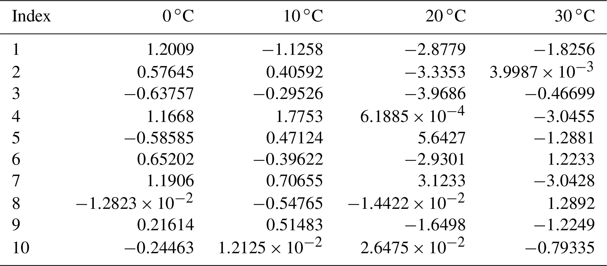
Table A2 Coefficients b₁₋₁₀ for the ratio A_DP∕A in Eq. (2). The coefficients were calculated for a 30^∘ elevation.

A1 Nonattenuated reflectivity and attenuation by rain

For the DSD of rain, we assume the widely used normalized gamma distribution (Illingworth and Blackman, 2002) as follows:

$$\begin{array}{}\text{(A2)}& n\left(D\right)={\displaystyle \frac{\mathrm{0.033}{N}_L{D}_{\mathrm{0}}^{\mathrm{4}}{\mathrm{\Lambda }}^{\mathit{\mu }+\mathrm{4}}}{\mathrm{\Gamma }(\mathit{\mu }+\mathrm{4})}}{D}^{\mathit{\mu }}\text{exp}(-\mathrm{\Lambda }D),\end{array}$$

where $\mathrm{\Lambda }=(\mathrm{3.67}+\mathit{\mu })/D_{\mathrm{0}}$, D is the equivalent sphere diameter in millimeters, D₀ is the median volume diameter in mm, N_L is the concentration parameter in mm⁻¹ m⁻³, and μ is the distribution shape parameter. For numerical calculations, we discretized the DSD, with D_i describing the mean diameter and N_i denoting the drop number of the ith size bin. D_i are equidistant from 10⁻² up to 8 mm, with a constant bin width of 10⁻² mm.

We approximate raindrops with oblate spheroids. The shape–size relation was taken from Pruppacher and Pitter (1971). Based on video disdrometer observations, Huang et al. (2008) showed that raindrops are mostly aligned horizontally, with a canting angle standard deviation of 8^∘. Aydin and Lure (1991) showed that this fluttering of drop orientation has a relatively small effect at 94 GHz. Even for the reflectivity difference between horizontal and vertical polarization for which one expects the effect of particle orientation to be maximum, the differences do not exceed 0.12 dB for rainfall rates up to 150 mm h⁻¹. In the following calculations, we therefore assume the raindrops to be horizontally aligned.

We calculate backscattering S_jk(D_i) and forward-scattering F_jk(D_i) coefficients using the T-matrix method (Mishchenko, 2000). Here, indices j and k stand for the polarization of transmitted and received waves, respectively. The temperature dependence of the refractive index of liquid water is taken from Ray (1972). Using S_hh(D_i) and F_hh(D_i), the nonattenuated reflectivity Z_i in mm⁶ m⁻³ and specific one-way attenuation due to liquid water A_i in dB km⁻¹ for one drop with the diameter D_i per unit volume are calculated with the following:

$$\begin{array}{}\text{(A3)}& Z_i={\displaystyle \frac{{\mathrm{10}}^{\mathrm{18}}{\mathit{\lambda }}^{\mathrm{4}}}{{\mathit{\pi }}^{\mathrm{5}}|K{|}^{\mathrm{2}}}}\left(\mathrm{4}\mathit{\pi }{\left|S_{\mathrm{hh}}\left(D_i\right)\right|}^{\mathrm{2}}\right),\end{array}$$

$$\begin{array}{}\text{(A4)}& A_i=\mathrm{8.686}\times {\mathrm{10}}^{\mathrm{3}}\left({\displaystyle \frac{\mathrm{2}\mathit{\pi }}{k}}\text{Im}\left[F_{\mathrm{hh}}\left(D_i\right)\right]\right),\end{array}$$

where $|K{|}^{\mathrm{2}}$ is the dielectric factor of liquid water, λ is the wavelength, and k is the wave number.

The final rainfall rate, reflectivity, and one-way attenuation are calculated as the sum over the DSD. The equations used for the different in situ instruments are summarized in Table A5.

A2 Gas attenuation

Unlike for longer wavelength radars (e.g., precipitation radars), gas attenuation cannot be neglected for the W band. The major contributions to gas attenuation at the W band are due to water vapor and oxygen, which we calculate with the model by Liebe (1989). As continuous profile information of temperature, water vapor, and pressure are unavailable at the RPG site and JOYCE-CF, we use the surface measurements of the weather station to approximate the vertical profiles. For the temperature profile, we use a constant empirical lapse rate K_t. Based on the radiosonde database from Essen (station no. 10410; 90 km from Meckenheim; 75 km from Jülich), the lapse rate K_t was estimated to be $\mathrm{4.8}\times {\mathrm{10}}^{-\mathrm{3}}$ K m⁻¹. The launches from 1 January 2010 to 23 October 2018 with surface relative humidity exceeding 65 % were used. For the K_t estimation, only the lowest 3 km of radiosonde ascends were taken. Relative humidity is assumed to be constant with height. The statistics of the calculated one-way gas attenuation profiles are shown in Fig. A1.

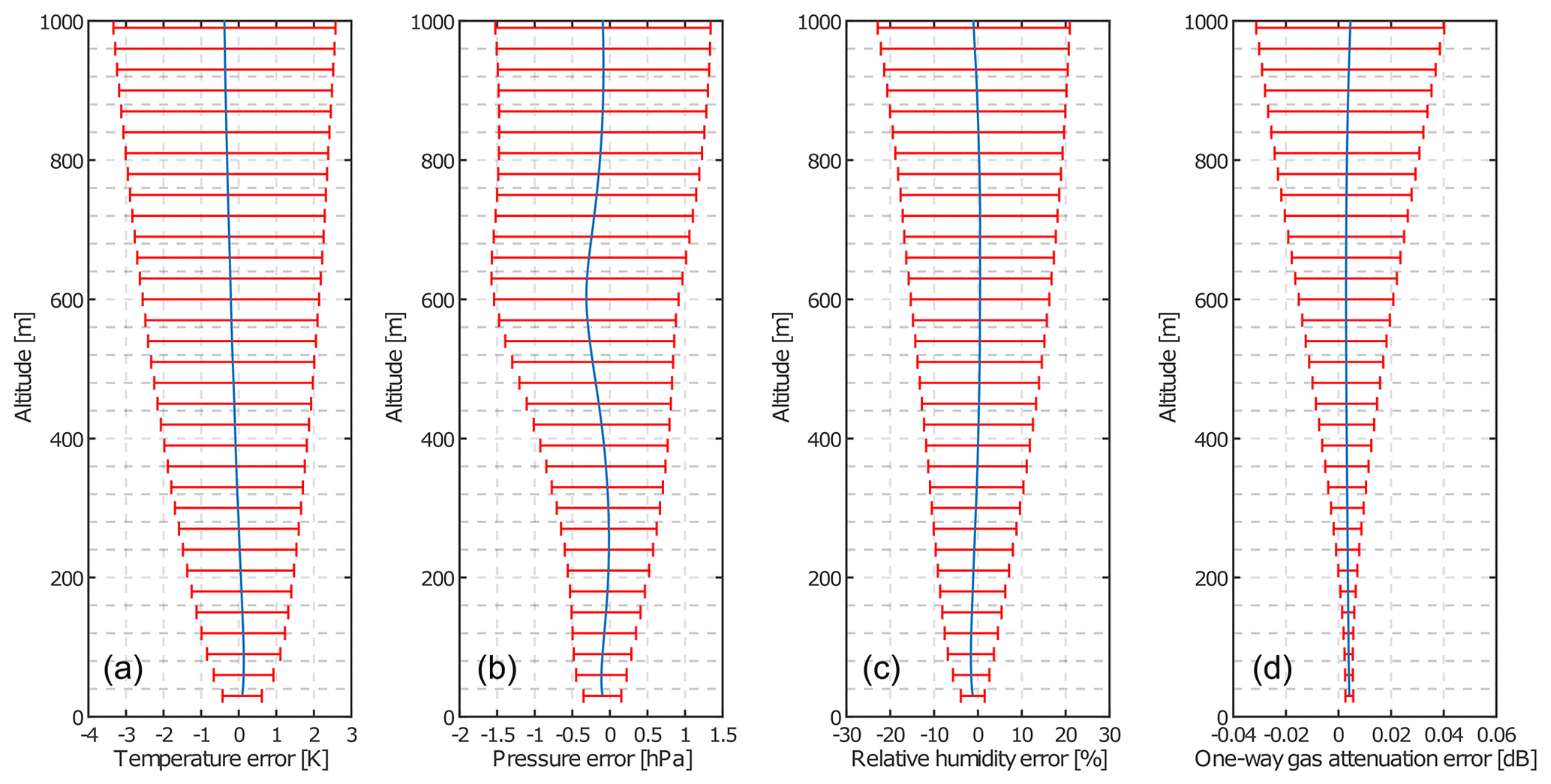
Figure A1 Uncertainties in the derived profiles of temperature (a), pressure (b), relative humidity (c), and one-way gas attenuation (d) when using only surface values from a weather station. The uncertainties have been estimated with a large set of radiosonde profiles restricted to a minimum surface relative humidity of 65%. The blue lines and the red bars show mean and ± 1 standard deviation of the corresponding difference, respectively.

A3 Drop evaporation

Xie et al. (2016) showed that a change in the drop size due to evaporation can be derived from the following equation:

$$\begin{array}{}\text{(A5)}& vD{\displaystyle \frac{\mathrm{d}D}{\mathrm{d}H}}=\mathrm{4}{\displaystyle \frac{S-\mathrm{1}}{F_K+F_D}},\end{array}$$

where D and v are the diameter and velocity of a drop, respectively, H is a vertical range traveled by the drop, S−1 is the supersaturation with respect to liquid water, and F_K and F_D are coefficients related to heat conduction and vapor diffusion, respectively. The calculation of F_K and F_D is based on Kumjian and Ryzhkov (2010).

Equation (A5) relates an initial drop size at a certain altitude to the drop size at the surface. The disdrometer-based method requires an opposite relation; i.e., what would the drop size be at a 250 m altitude if its size at the surface is known? The relation can also be found by solving Eq. (A5). The equation is solved numerically for surface diameters D_s from 0.06 to 3 mm, with a grid of 0.01 mm, using an iterative approach. Large drops are less influenced by evaporation (Xie et al., 2016); therefore, for drops larger than 3 mm, the size change is neglected. The surface drop size is taken as the first guess of the drop size at 250 m D₂₅₀. Using Eq. (A5), the corresponding size at the surface D_sm is calculated and compared with D_s. In case the difference is smaller than 0.01 mm, D₂₅₀ is taken as the solution for corresponding D_s. If the difference is larger, D₂₅₀ is changed until the condition is satisfied. For a minimization of the difference, the differential evolution method (Das et al., 2009) is applied, although any other optimization algorithm can be also used. Even though the convergence for a single size is fast, the application of such evaporation correction to a number of sizes and different environment conditions is time consuming. Therefore, a set of precalculated D_s–D₂₅₀ relations at surface temperatures from 0 to 20 ^∘C, with the 5 ^∘C step, and surface relative humidity from 60 % to 100 %, with the 5 % step at the 1000 hPa surface pressure, is used for the D_s–D₂₅₀ function approximation as follows:

$$\begin{array}{}\text{(A6)}& \begin{array}{rl}{D}_{\mathrm{250}}(D_{\mathrm{s}},T,\mathrm{RH})& =\left[\sum _{i=\mathrm{1}}^{\mathrm{10}}{g}_{i}f(p_i{D}_{\mathrm{s}}+q_{i}T+u_i\mathrm{RH}+{\mathit{\alpha }}_i)\right]\\ & +\mathit{\beta },\text{if}\mathrm{0}<D_{\mathrm{s}}<\mathrm{3}\mathrm{mm}{D}_{\mathrm{s}},\text{if}{D}_{\mathrm{s}}\ge \mathrm{3}\mathrm{mm},\end{array}\end{array}$$

where D₂₅₀ and D_s are in millimeters, T is in degrees Celsius and has to be in the range from 0 to 30 ^∘C, and RH is in percent and should be in the range from 60 % to 100 %. The coefficients g, p, q, u, and α are given in Table A4, β=20.038. For the given ranges of the input parameters, the root mean square difference between the simulated and approximated values of D₂₅₀ is 5.8 µm. In the Supplement, we provide a MATLAB and Octave function for Eq. (A6).

Table A3 Coefficients c₁₋₁₇ for A in Eq. (3). The coefficients were calculated for a 30^∘ elevation.

Table A4 Coefficients for D₂₅₀ in Eq. (A6).

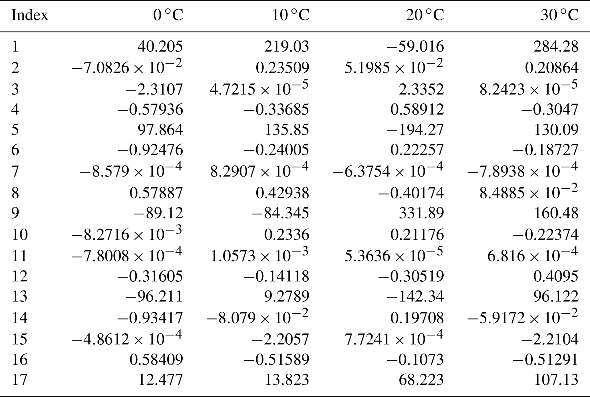
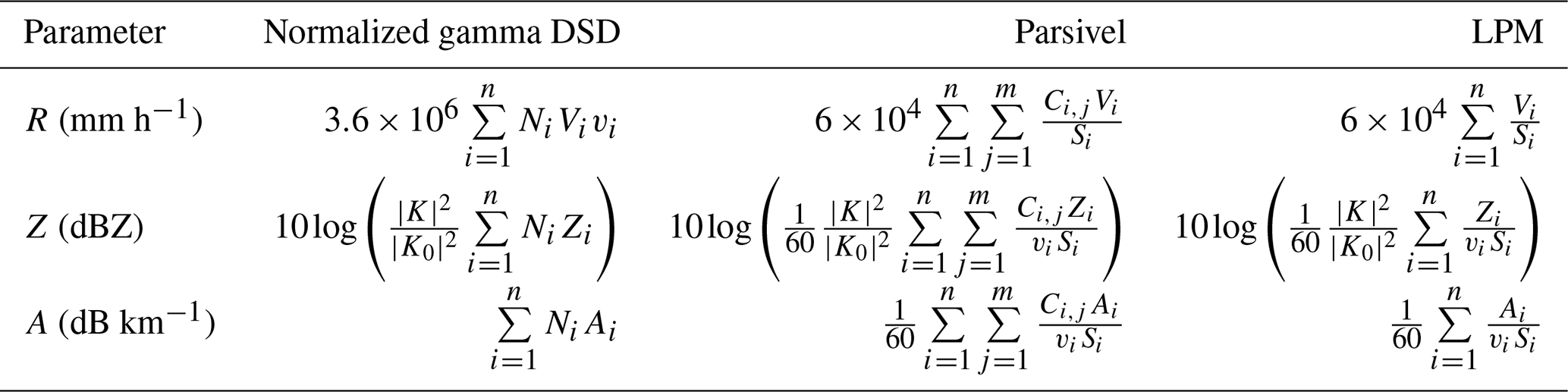
Table A5 Summary of calculation formulas for rain rate, reflectivity, and attenuation for the normalized gamma DSD, DSD from Parsivel, and drops detected by LPM. For the normalized gamma DSD and Parsivel, the index i ranges over n diameter bins, while for LPM it varies over n drops detected by the instrument 1 min prior to a radar sample time. The index j moves over m velocity bins of Parsivel. C_i,j is the cell of the Parsivel raw data matrix. N_i is a number of particles in the diameter bin i. V_i and v_i are volume in cubic meters and terminal velocity in meters per second of a drop with the diameter D_i, respectively. Z_i and A_i are reflectivity and attenuation for one drop, with the diameter D_i in a unit volume, respectively. $S_i=L_{\mathrm{b}}(W_{\mathrm{b}}-D_i/\mathrm{2})$ is the effective sampling area in square meters of a disdrometer, with L_b and W_b being the length and the width of the disdrometer laser beam (Tokay et al., 2014). $|K{|}^{\mathrm{2}}$ is the dielectric factor of water at a certain temperature. $|K_{\mathrm{0}}{|}^{\mathrm{2}}=\mathrm{0.74}$ is the constant dielectric factor of water at 8^∘C set in the processing routine of the used radars.

Appendix B: Polarimetric variables

The T-matrix calculations are also used to derive polarimetric variables such as backscattering differential reflectivity z_DR (dB), backscattering differential phase δ (^∘), one-way differential attenuation A_DP (dB km⁻¹), and specific differential phase K_DP (^∘ km⁻¹) as follows:

$$\begin{array}{}\text{(B1)}& {\displaystyle }{z}_{\mathrm{DR}}=\mathrm{10}{\log }_{\mathrm{10}}\left({\displaystyle \frac{\sum _{i=\mathrm{1}}^n{\left|S_{\mathrm{hh}}\left(D_i\right)\right|}^{\mathrm{2}}{N}_i}{\sum _{i=\mathrm{1}}^n{\left|S_{\mathrm{vv}}\left(D_i\right)\right|}^{\mathrm{2}}{N}_i}}\right),\text{(B2)}& {\displaystyle }\mathit{\delta }={\displaystyle \frac{\mathrm{180}}{\mathit{\pi }}}\arg \left[\sum _{i=\mathrm{1}}^n{N}_i{S}_{\mathrm{hh}}^{*}\left(D_i\right)S_{\mathrm{vv}}\left(D_i\right)\right],\text{(B3)}& {\displaystyle }\begin{array}{rl}{A}_{\mathrm{DP}}& =\mathrm{8.686}\times {\mathrm{10}}^{\mathrm{3}}{\displaystyle \frac{\mathrm{2}\mathit{\pi }}{k}}\sum _{i=\mathrm{1}}^n\text{Im}\left[F_{\mathrm{hh}}\left(D_i\right)\right.\\ & \left.-F_{\mathrm{vv}}\left(D_i\right)\right]N_i,\end{array}\text{(B4)}& {\displaystyle }{K}_{\mathrm{DP}}={\mathrm{10}}^{\mathrm{3}}{\displaystyle \frac{\mathrm{180}}{\mathit{\pi }}}{\displaystyle \frac{\mathrm{2}\mathit{\pi }}{k}}\sum _{i=\mathrm{1}}^n\text{Re}\left[F_{\mathrm{hh}}\left(D_i\right)-F_{\mathrm{vv}}\left(D_i\right)\right]N_i,\end{array}$$

where ^∗ denotes the complex conjugation.

Differential reflectivity Z_DR(r) (dB) and differential phase Φ_DP(r) (^∘) at a certain range r (km) from the radar are the sum of corresponding backscattering and propagational components as follows:

$$\begin{array}{}\text{(B5)}& {\displaystyle }{Z}_{\mathrm{DR}}\left(r\right)=z_{\mathrm{DR}}\left(r\right)+\underset{\mathrm{DA}\left(r\right)}{\underbrace{\mathrm{2}\underset{\mathrm{0}}{\overset{r}{\int }}-A_{\mathrm{DP}}\left(r\right)\mathrm{d}r}},\text{(B6)}& {\displaystyle }{\mathrm{\Phi }}_{\mathrm{DP}}\left(r\right)=\mathit{\delta }\left(r\right)+\underset{\mathrm{DP}\left(r\right)}{\underbrace{\mathrm{2}\underset{\mathrm{0}}{\overset{r}{\int }}{K}_{\mathrm{DP}}\left(r\right)\mathrm{d}r}},\end{array}$$

where DA and DP are propagation components in differential reflectivity and differential phase, respectively.

Appendix C: Variance of a numerical average

A variance (denoted as var) of an average of N_s samples can be found as follows:

$$\begin{array}{}\text{(C1)}& \text{var}\left({\displaystyle \frac{\mathrm{1}}{N_{\mathrm{s}}}}\sum _{i=\mathrm{0}}^{N_{\mathrm{s}}-\mathrm{1}}{s}_i\right)={\displaystyle \frac{\mathrm{1}}{N_{\mathrm{s}}^{\mathrm{2}}}}\sum _{i=\mathrm{0}}^{N_{\mathrm{s}}-\mathrm{1}}\sum _{j=\mathrm{0}}^{N_{\mathrm{s}}-\mathrm{1}}\text{cov}(s_i,s_j),\end{array}$$

where cov stands for covariance, s is a sample with a lag is indicated by the subscripts i and j. The covariance cov(s_i,s_j) is calculated as a multiplication of the standard deviations of the corresponding variables and their correlation. Assuming that the analyzed process is stationary with the standard deviation σ_s, cov(s_i,s_j) can be written as follows:

$$\begin{array}{}\text{(C2)}& \text{cov}(s_i,s_j)={\mathit{\rho }}_{\mathit{\tau }}{\mathit{\sigma }}_s^{\mathrm{2}}.\end{array}$$

Here ρ_τ is the normalized autocovariance function at the lag $\mathit{\tau }=i-j$. Substituting Eq. (C2) into Eq. (C1) as follows:

$$\begin{array}{}\text{(C3)}& \text{var}\left({\displaystyle \frac{\mathrm{1}}{N_{\mathrm{s}}}}\sum _{i=\mathrm{0}}^{N_{\mathrm{s}}-\mathrm{1}}{s}_i\right)={\displaystyle \frac{{\mathit{\sigma }}_{\mathrm{s}}^{\mathrm{2}}}{N_{\mathrm{s}}^{\mathrm{2}}}}\sum _{i=\mathrm{0}}^{N_{\mathrm{s}}-\mathrm{1}}\sum _{j=\mathrm{0}}^{N_{\mathrm{s}}-\mathrm{1}}{\mathit{\rho }}_{\mathit{\tau }}.\end{array}$$

A similar relation for analytic functions was derived by Leith (1973). In the case of uncorrelated samples, the normalized autocovariance function is a delta function, the double sum in Eq. (C3) is equal to N_s, and the variance can be found using the well-known relation ${\mathit{\sigma }}_{\mathrm{s}}^{\mathrm{2}}/N_{\mathrm{s}}$. This relation is widely used in the weather radar community to improve the signal detection (Eq. 5.193 in  Bringi and Chandrasekar, 2001; Görsdorf et al., 2015). In contrast, when all the samples are highly correlated within the averaging period, the double sum is equal to $N_{\mathrm{s}}^{\mathrm{2}}$, and as expected, the variance of the average does not change. In the general case, when the analyzed process has a certain coherency time, the variance is within the range between ${\mathit{\sigma }}_{\mathrm{s}}^{\mathrm{2}}/N_{\mathrm{s}}$ and ${\mathit{\sigma }}_{\mathrm{s}}^{\mathrm{2}}$.