the Creative Commons Attribution 4.0 License.
the Creative Commons Attribution 4.0 License.
 | 20 Nov 2020
Filtering of pulsed lidar data using spatial information and a clustering algorithm
Wind lidars present advantages over meteorological masts, including simultaneous multipoint observations, flexibility in measuring geometry, and reduced installation cost. But wind lidars come with the “`cost” of increased complexity in terms of data quality and analysis. Carrier-to-noise ratio (CNR) has been the metric most commonly used to recover reliable observations from lidar measurements but with severely reduced data recovery. In this work we apply a clustering technique to identify unreliable measurements from pulsed lidars scanning a horizontal plane, taking advantage of all data available from the lidars – not only CNR but also line-of-sight wind speed (VLOS), spatial position, and VLOS smoothness. The performance of this data filtering technique is evaluated in terms of data recovery and data quality against both a median-like filter and a pure CNR-threshold filter. The results show that the clustering filter is capable of recovering more reliable data in noisy regions of the scans, increasing the data recovery up to 38 % and reducing by at least two-thirds the acceptance of unreliable measurements relative to the commonly used CNR threshold. Along with this, the need for user intervention in the setup of data filtering is reduced considerably, which is a step towards a more automated and robust filter.
- Article
(3493 KB) - Full-text XML
- BibTeX
- EndNote


Long-range scanning wind lidars are useful tools, and their adoption has grown rapidly in recent years in wind energy applications (Vasiljević et al., 2016). Scanning wind lidars can measure time evolution and spatial characteristics of wind fields over large domains at a lower cost of installation than meteorological masts. Nevertheless, atmospheric conditions and instrument noise can have an important impact on the data quality. For long-range scanning lidars this becomes an important issue due to the lack of additional instruments placed over the measurement area that would be useful to compare data quality since noise can contaminate large portions of the scanning domain. The most commonly used criterion to retrieve reliable observations is a threshold on values of the carrier-to-noise ratio, CNR, threshold that will depend on site conditions, experimental setup, and the instrument manufacturer (Gryning et al., 2016; Gryning and Floors, 2019). Even though the CNR threshold retrieves quality observations, its application might result in large numbers of good data rejected in regions far from the instrument, where CNR has decreased rapidly with distance. To cope with this issue Meyer Forsting and Troldborg (2016) and Vasiljević et al. (2017) have proposed filters based on the smoothness and continuity of the wind field. Such filters work by detecting discrete or anomalous steps (above a certain threshold predefined by the user) in line-of-sight wind speed, VLOS, compared to its local (moving) median. Beck and Kühn (2017) first and then Karagali et al. (2018), in an adapted version, follow a different approach (here called a KDE filter, from kernel density estimate) based on the statistical self-similarity of the data, which, in simple terms, means that reliable observations are alike and will be located close together in the observational space. The probability density distribution of observations (estimated via KDE) in a dynamically normalized VLOS−CNR space shows that measurements likely to be valid are located in a high-data-density region. Observations sparsely distributed beyond a boundary defined by a threshold in the acceptance ratio or the ratio between the probability density of any observation and the maximum probability density over the whole set of measurements are finally identified as noise. Both approaches need the definition of one or more thresholds and a window size, either in time for the KDE filter or in space for the wind field smoothness approach. These parameters are dependent on different characteristics of the data, like the lidar scanning pattern for instance.
Both approaches miss important and complementary information, either neglecting the strength of the signal backscattering (quantified by CNR) or the spatial distribution and smoothness of the wind field. Moreover, in both approaches the position of observations is not taken into account, information that can shed light on areas permanently showing anomalous values of VLOS or CNR, like hard targets. Including all these features within the smoothness approach is difficult since CNR is not a smooth field like VLOS. Moreover, considering smoothness and position in the KDE filter results in a computationally costly kernel density estimation if we look for an optimal bandwidth parameter in a higher-dimensional space with a fine resolution of the kernel density estimate.
Data self-similarity – over any scale in the case of fractals or a range of them in real situations (Mandelbrot, 1983) – is closely related to clustering techniques (Backer, 1995), which can classify large data sets with many different features at a relatively low computational cost. The KDE filter approach shares some characteristics with the popular k-means clustering algorithm MacQueen (1967) since they define one (or several for k-means) specific group of data belonging to a unique category (or cluster) whose size and location in the observational space will depend on data density or, more specifically, on a kernel density estimation. The main difference between these two algorithms is the way they treat sparse data points that fall in low-density regions. Unlike the KDE filter, which rejects noise via the acceptance ratio, the k-means clustering algorithm assigns sparse points to the cluster with the nearest center no matter if they are outliers or present unlikely values from a physical point of view.
The Density Based Spatial Clustering for Applications with Noise algorithm, or DBSCAN (Ester et al., 1996; Pedregosa et al., 2011), introduced in
Sect. 4.3, presents several advantages over k-means in detecting clusters in a higher dimensional space: it introduces the notion
of noise or sparsely distributed observations, it does not need prior knowledge of the number of clusters in the data and it is capable of identifying
clusters of arbitrary shape. To the best of our knowledge, this is the first time that this type of clustering algorithm is applied to identify nonreliable observations from pulsed lidars. This approach, which can be understood as a natural extension of the KDE filter, is compared to the
smoothness-based filter on two types of data: synthetic wind fields data as a controlled test case and real data.
This paper is organized as follows: Sect. 2 describes the real data used to test the different filtering approaches, and Sect. 3 presents the synthetic data used during a controlled test as well as the methodology to obtain it. Section 4 then gives a description of the different filters applied in this study to both data sets to continue with the definition of the performance tests in Sect. 5. In Sect. 6 the performance tests are presented along with a discussion on their validity and quality. Section 7 discusses the quality of the methodology behind the tests and the advantages and disadvantages of the proposed approach. Section 8 presents the conclusions of this study.
The filtering techniques presented here were tested on lidar measurements made at the Test Centre Østerild located in northern Jutland, Denmark (see Fig. 1). Known as the Østerild balconies experiment (Mann et al., 2017; Karagali et al., 2018; Simon and Vasiljevic, 2018), this measuring campaign aimed to characterize horizontal flow patterns above a flat, heterogeneous forested landscape at two heights relevant for wind energy applications, covering an area of around 50 km2 and a wide range of scales in both time and space.
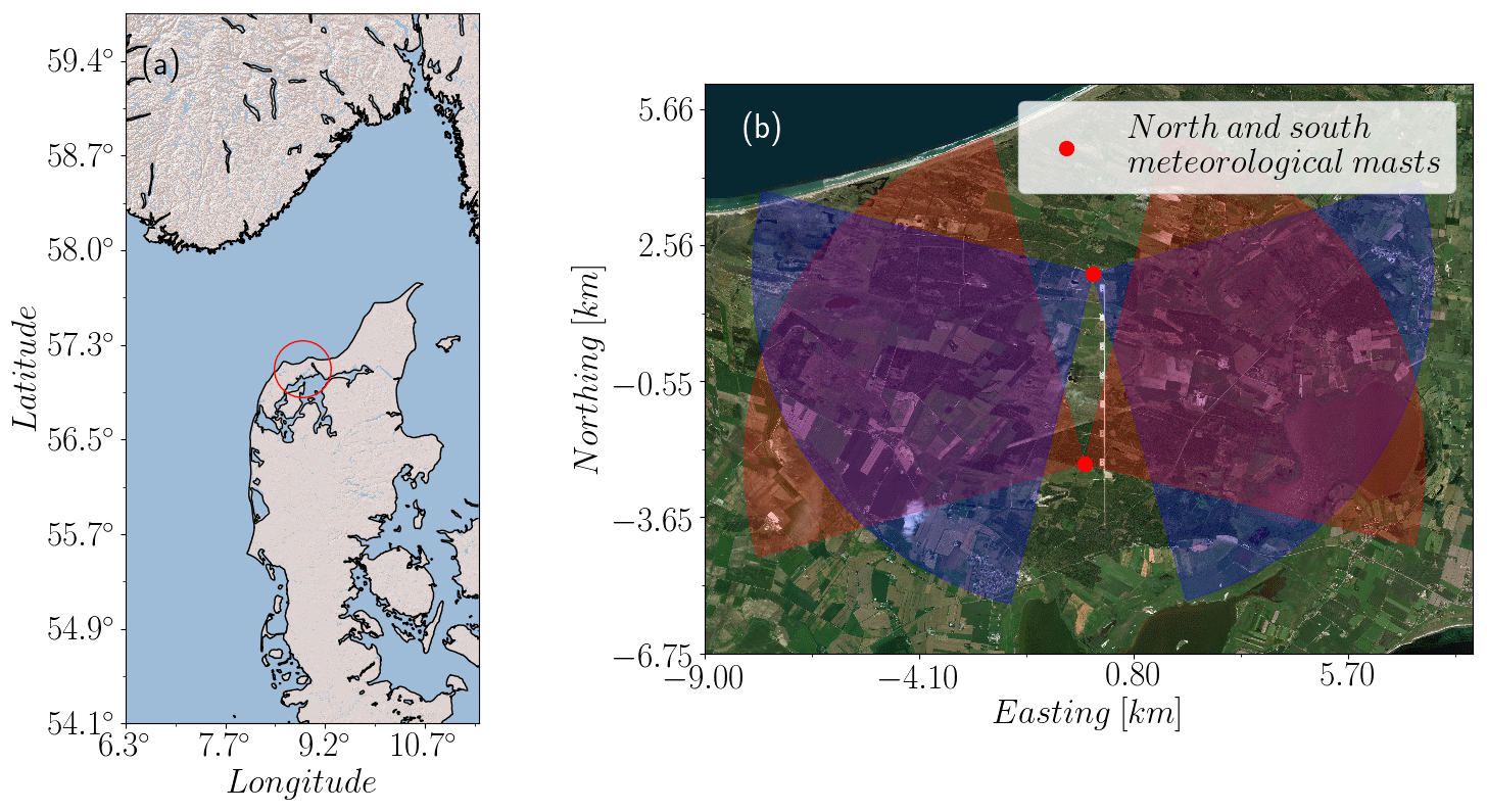
Figure 1(a) Location of the Østerild turbine test center, place of the balconies experiments, northern Jutland, Denmark (© 2009 Esri). (b) Detail of the test center site, with the location of the meteorological masts where north (blue) and south (red) WindScanners were installed. During the measurement campaign the PPI scans both pointed west in some periods and east in others (© 2017 DigitalGlobe, Inc.).
Table 1Characteristics of the balconies experiment, from Karagali et al. (2018). The scans are neither instantaneous nor totally synchronous, with a horizontal sweep speed of 2 in the azimuth direction in a range of 90∘ and a total time of 45 s per scan.
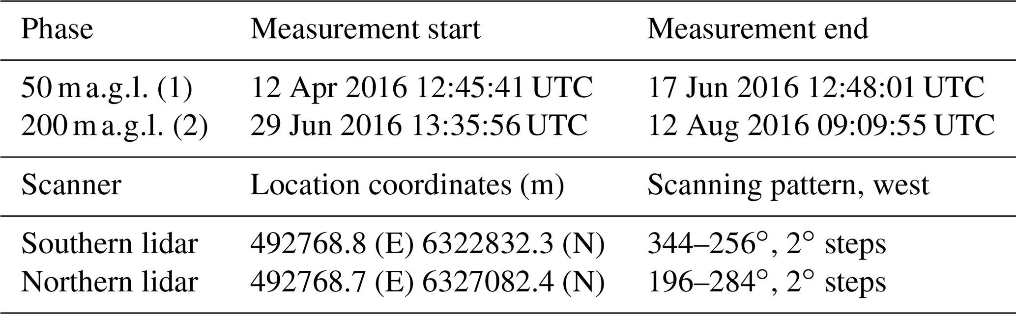
The experiment consist of two measuring phases (see Table 1) with two long-range WindScanners performing plan position indicator (PPI) scanning patterns, aligned in the north–south axis and installed at 50 during phase 1 and 200 in phase 2. WindScanners (Vasiljević et al., 2016) consist of two or more spatially separated lidars, which are synchronized to perform coherent scanning patterns, allowing the retrieval of two- or three-dimensional velocity vectors at different points in space. These experiments were conducted between April and August of 2016 (Simon and Vasiljevic, 2018). In each phase, the northern and southern lidars scanned in the west and east direction relative to the corresponding meteorological masts where they were installed. The data used in this study originated from both phases of the experiment, with PPIs pointing to the west. For more details about the experiment, lidars, and terrain characteristics see Karagali et al. (2018), Vasiljević et al. (2016), and Simon and Vasiljevic (2018).
This data set is well suited to test different data filtering techniques. A large measurement area will be affected by local terrain and atmospheric conditions, like clouds or large hard targets. Moreover, at this scale lidars reach their measuring limitations since the backscattering from aerosols decreases rapidly with distance (Cariou, 2015).
Assessing and comparing the performance of filters is challenging with no reference available to verify that rejected or accepted observations are reliable or bad observations. This is especially difficult for long-range scanning lidars since their measurements cover large areas and, due to spatial variability, a valid reference would need several secondary anemometers scattered over the scanning area. Testing filters on a controlled and synthetic data set contaminated with well-defined noise presents an option to deal with this problem. In this study, the filters presented in Sect. 4 are tested on individual scans sampled from synthetic wind fields generated using the Mann turbulence spectral tensor model (Mann, 1994) and contaminated with procedural noise (Perlin, 2001).
3.1 Synthetic-wind-field generation
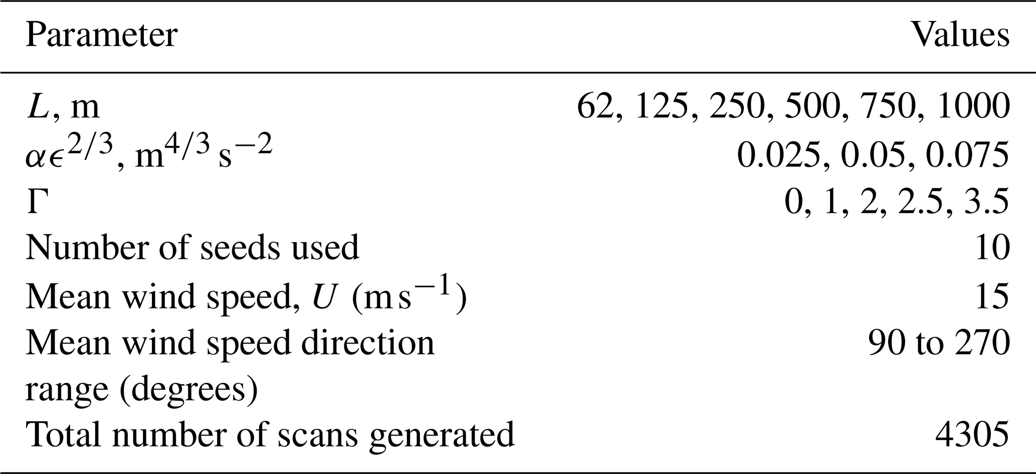
Synthetic PPI scans are sampled by a lidar simulator from synthetic wind fields generated via the Mann model (Mann, 1998) in a horizontal, two-dimensional square domain of 2048 × 2048 grid points, with dimensions of 9200 m × 7000 m. The generated turbulence fields are the result of input parameters of the turbulence spectral tensor model, namely length scale, L; turbulence energy dissipation, αϵ2∕3; and anisotropy, Γ. The fields generated correspond to wind speed fluctuations, to which the desired mean wind speed is subsequently added. Depending on the initial random seed used, different wind field realizations with the exact same turbulence statistics can be generated. For details on wind field generation using the Mann model, refer to Mann (1998). Table 2 shows the range of values used for the generation of two-dimensional wind fields. Large values of αϵ2∕3 or small-scale turbulence, for instance, mean that sudden spatial changes in wind speed are more likely, which increase the false identification of outliers. Mean wind direction, turbulence anisotropy, and length scale will also affect the sampling due to the lidars' measuring characteristics.
3.2 Lidar simulator
Lidar simulators have been presented previously by Stawiarski et al. (2013) and Meyer Forsting and Troldborg (2016). They sample VLOS values from wind fields generated via large-eddy simulation (LES), mimicking the operational principle of lidars by proper time and spatial (probe volume) averaging of the background wind field. The lidar simulator presented here follows the same principles, this time sampling from synthetic wind fields generated via the Mann model.
Table 3The characteristics of the lidar simulator and real long-range lidar (Karagali et al., 2018; Vasiljević et al., 2016) used for the controlled test of the filters.
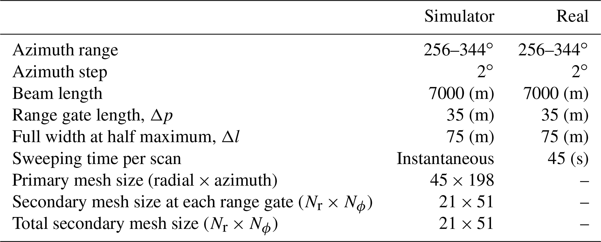
The simulator receives scanning pattern characteristics as input (beam range, range gate step, azimuth angle range, and azimuth angle steps) to generate a primary mesh with the sampling positions on top of background wind field. Following the measuring principle of the lidar, the VLOS observed at each position in this mesh will represent averages of a continuum along each range gate step (due to probe volume averaging) and an average of many azimuth positions within the azimuth step due to the almost continuous sweep of the lidar's beam. The simulator mimics this by generating a secondary, refined mesh with Nr points in each range gate and Nϕ beams within each azimuth step. The background wind field components, U and V, are then interpolated on this secondary mesh and projected on each refined beam to obtain VLOS using Eq. (1), with θ being the corresponding beam azimuth angle.
The final step is the spatial (probe volume) averaging and the azimuth (sweeping) averaging around each position in the primary mesh. Spatial averaging is done by applying a weighting function to all VLOS values along each refined beam. The weighting function used here is defined in Eq. (2), as in Banakh and Smalikho (1997) and Smalikho and Banakh (2013). This function will assign weights to each point in the refined beam according to its distance to the range gate position in the primary mesh, F, and the instrument probe volume parameters, namely, range gate length, Δp, and full width at half maximum, Δl (cf. Table 3). Here, Erf(x) is the error function, and rp is the beam width contribution to the volume averaging.
The azimuth averaging is the arithmetic mean of the Nϕ values of VLOS at each range gate after spatial averaging. It represents the accumulation information of the backscattered signal spectra as they sweep an azimuth sector before estimation of the spectral peak and VLOS.
3.3 Synthetic noise generation
The most simple noise that can be used to contaminate synthetic scans are sparse, uniformly distributed outliers. This noise, also known as salt-and-pepper noise, is easily detected and eliminated by median-like filters when extreme; discrete steps affect the smoothness of an image (Huang et al., 1979; Burger and Burge, 2008). Nevertheless, noise in real scans comes as regions of anomalously high and/or low VLOS, and they can pass through the filter undetected. Procedural noise, introduced by Perlin (2001) to recreate synthetic textures on surfaces for computer graphics applications, creates regions of coherent noise that better resembles the spatial distribution of scanning lidars' measurements. For the two-dimensional case, the procedural noise function N(x,y) maps two-dimensional coordinates, (x,y), onto the range as follows,
-
A two-dimensional grid of m by n elements is generated, and a pseudorandom, two-dimensional unit gradient, , is assigned to each grid point (xi,yj). The pseudorandomness rises from the fact that gij are picked from a precomputed list of gradients with length . We select values from this list using the index permutation grid , also with m×n elements. Then, gij will correspond to the gradient in the position pij of the precomputed list. Elements pij are shuffled for each realization.
-
For each grid point (xi,yj) enclosing (x,y), a distance vector is generated.
-
Finally, the noise function is the sum of dot products, , for q grid points surrounding (x,y). Weights wq correspond to , and C is a normalization constant to ensure that .
The function N(x,y) allows the generation of noisy regions, than can be distributed according to backscatter decay with distance. Three bands centered at 50 %, 70 %, and 90 % of the total beam length (and spanning the entire azimuth range) have an increasing fraction of noise, contaminating 30 %, 60 %, and 90 % of the observation, respectively. The noise amplitude is 35 (m s−1), the limit of the observable range for the instruments described in Sect. 2. Figure 2c shows one contaminated scan and its increasing contaminated area as we move along the beams. The same figure shows the distribution of the noise generated by the algorithm after scaling and the probability distribution of contaminated synthetic VLOS compared to real data with low values of CNR. The distribution of real data presents heavier tails than the ones generated, with higher probability of observing extreme values of VLOS. Modeling real noise is difficult since the process that generates it depends on the measuring principle of the lidar and atmospheric conditions. The synthetic noise used here does not intend to be totally realistic but more subtle and smoother than the one observed in real measurements, making the identification of contaminated points more difficult.
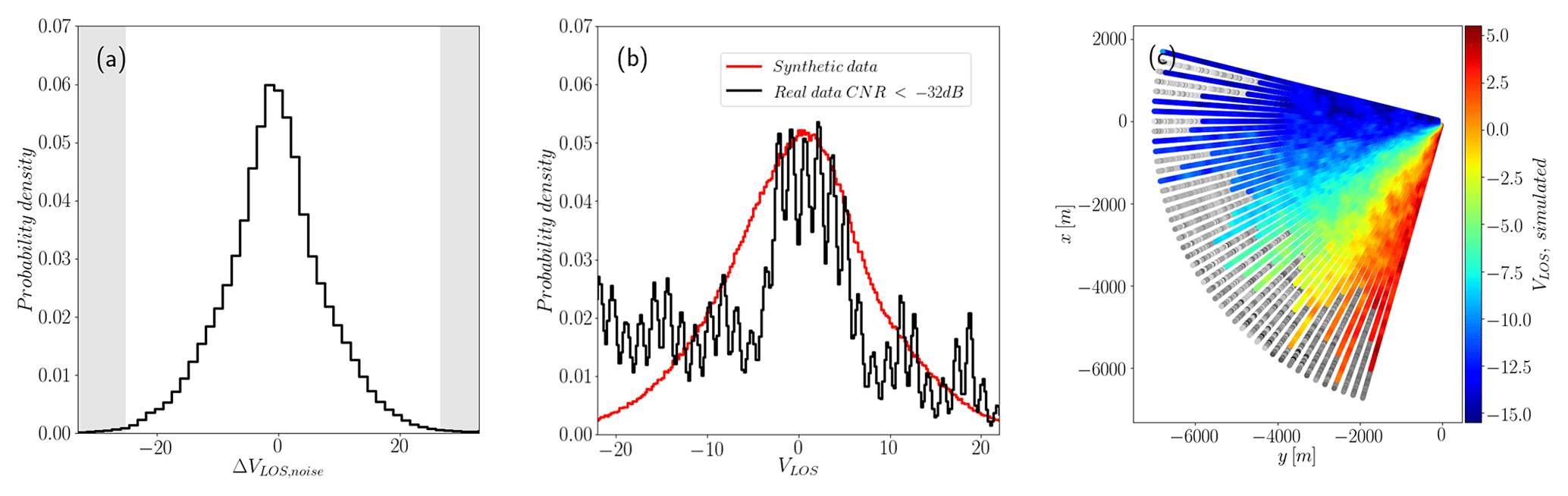
Figure 2Procedural noise on synthetic scans. (a) Distribution of ΔVLOS, noise, the noise added. Maximum values are within the observable range [−35, 35] (m s−1). (b) Distribution of real VLOS with low CNR values (black) and contaminated, synthetic VLOS+ΔVLOS, noise (red) for a mean wind direction facing the scan. (c) Individual scan showing the increasing fraction of added noise (gray) with distance.
4.1 CNR threshold
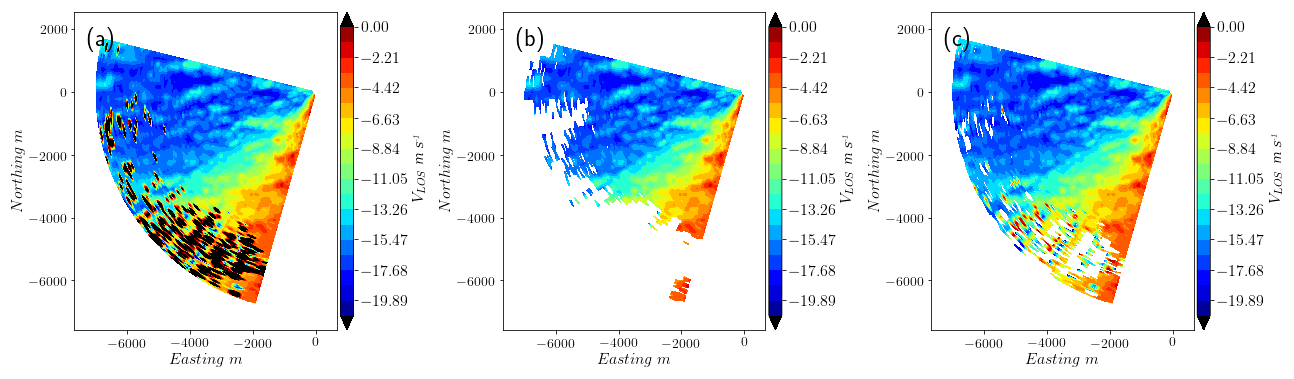
CNR thresholds are well known, and lidar manufacturers usually recommend values for rejection of signals with poor backscattering or hitting hard targets (Cariou, 2015). However, the selection of an appropriate threshold for CNR that assures data quality and good data recovery is not easy. Figures 3 and 4 show data from a scan with noisy observations from CNR values below −27 dB. Both extreme and limited values of VLOS show low CNR values in the distant region of the scan and data loss results after the application of the CNR threshold (Fig. 4b). When a limit to VLOS is applied instead, Fig. 4c shows that the smoothness in VLOS is lost in the lower part of the scan. A conservative threshold of −24 dB is used here since the resulting VLOS probability distribution shows very few outliers, and it can be used as a reference when the performance of the filters proposed is compared.
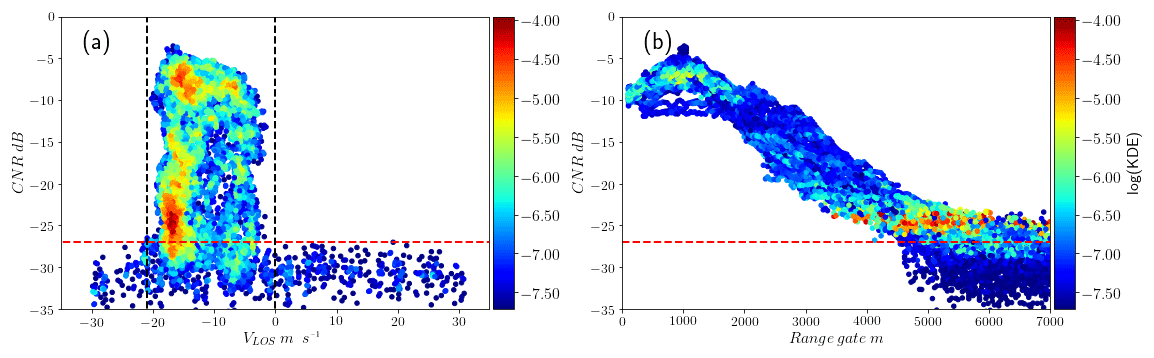
Figure 3(a) CNR and VLOS for one scan from the balconies experiment, including the probability density (KDE). Observations with CNR > −27 dB (dashed red line) show a limited range of VLOS (dashed black line). A portion of observations with high probability density remains in the rejection area. (b) CNR v∕s distance for the same data. Observations with low CNR values and high probability density can be found in the distant region of the scan.
4.2 Median-like filter
The median filter arises as a viable option for detecting erroneous measurements since it is well known that this type of nonlinear filter is suited to detect and filter noise that presents distributions with large tails. Here we use an adaptation of the traditional median filter used in the image-processing community, closely related to the three-stage filtering technique described in Menke et al. (2019): observations are not replaced by the local moving median but excluded if the absolute difference between their value and the local moving median is above a certain threshold, ΔVLOS, threshold. Unlike Huang et al. (1979), the two-dimensional moving window is replaced by two one-dimensional window instances, the first in the line of sight or the radial direction, r, and finally in the azimuth direction, θ, considering the polar coordinates of the scan. This simplification reduces the computation time significantly.
The input parameters of this filter will be the size (or number of elements) of the moving windows in the radial and azimuth directions, nr and nϕ, respectively, and ΔVLOS, threshold. For fixed values of ΔVLOS, threshold, nr, and nϕ, the spatial structure of wind speed fluctuations will have an important effect on the recovery rate and noise detection of this filter. A sensitivity analysis carried out using the metrics presented in Sect. 5.1 on the synthetic data set shows that the optimal set of parameters is nr = 5, nϕ = 3, and ΔVLOS, threshold = 2.33 m s−1 (See Appendix A). This set is used for both artificial and real data. The filter does not include a time window, and it is applied to individual scans.
4.3 Filtering using a clustering algorithm
If we represent lidar observations as m-dimensional vectors, with m the number of features or parameters of the data, measurements not affected by
poor backscattering or noise will cluster together in regions of high data density, as shown in Figs. 3 and 4. The
approach presented here identifies such clusters applying DBSCAN to data described by CNR, VLOS, and, additionally, spatial
location and smoothness features, which help to make clusters more distinguishable.
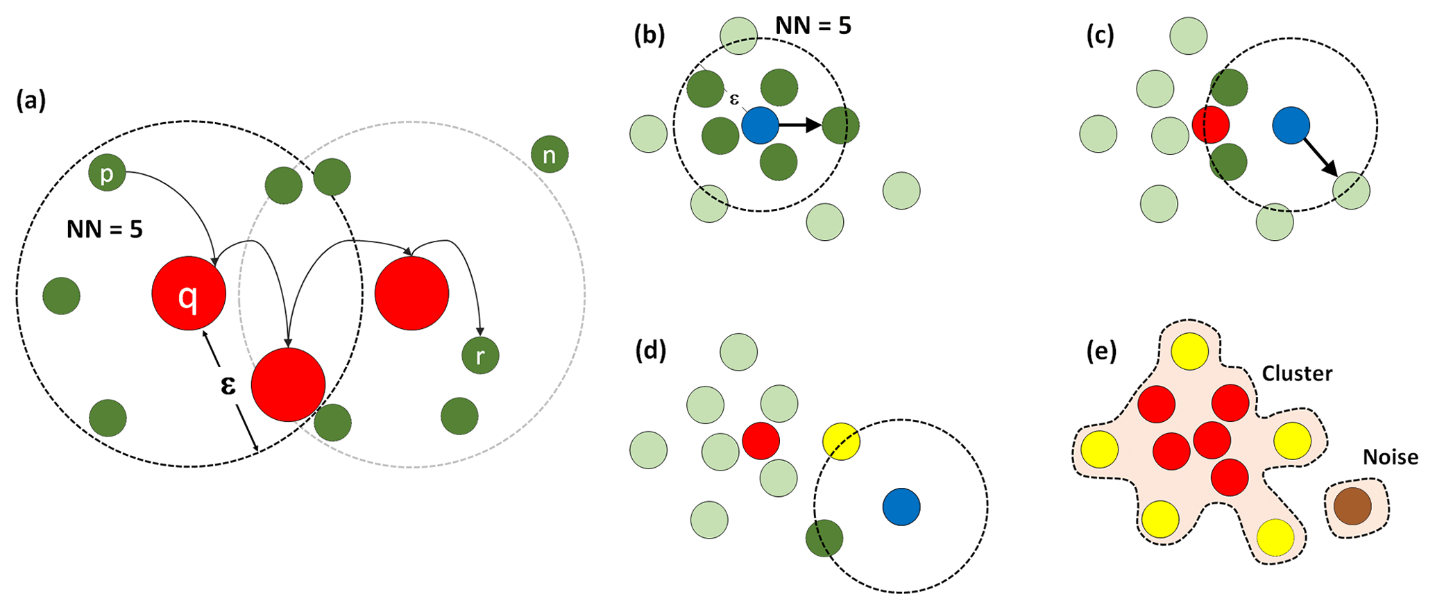
Figure 5(a) DBSCAN algorithm definitions: direct density-reachable point p (reachable by the core point q) and density-reachable and density-connected points p and r. Here point n does not belong to any of these categories but noise. The DBSCAN algorithm working: (b) the current point being evaluated has the minimum number of nearest neighbors required, NN, within a neighborhood of size ε, classified as a core point (red). (c) The next point has fewer than NN neighbors, but one of them is a core point and becomes a border point (yellow). (d) A point with neither NN neighbors nor core points within ε, classified as noise (brown). (e) The final cluster and noise. The former is a collection of density-connected points.
DBSCAN identifies clusters and noise based on two parameters: a neighborhood size, ε, and a minimum number of nearest
neighbors, NN. The parameter ε is the Euclidean distance from one observation to the limits of a neighborhood that might contain
NN (or more) nearest neighbors. Intuitively, these parameters will define the minimum density that a group of data points needs to have to be
identified as a cluster. Observations within a cluster fall into the following categories.
-
Core point: points q whose ε neighborhood contains NN or more points.
-
Direct density-reachable point: points p which are reachable by q by lying within its ε neighborhood.
-
Density-reachable point: points p reachable by a point r through one or a set of directly connected core points q.
DBSCAN travels across data points identifying core points, border points (density-reachable points with at least one core point within the
ε neighborhood) and noise, or points that do not belong to any of the categories described above. Finally, the algorithm separates
clusters as individual groups of density-connected points. Figure 5 schematically shows these definitions and how the algorithm works.
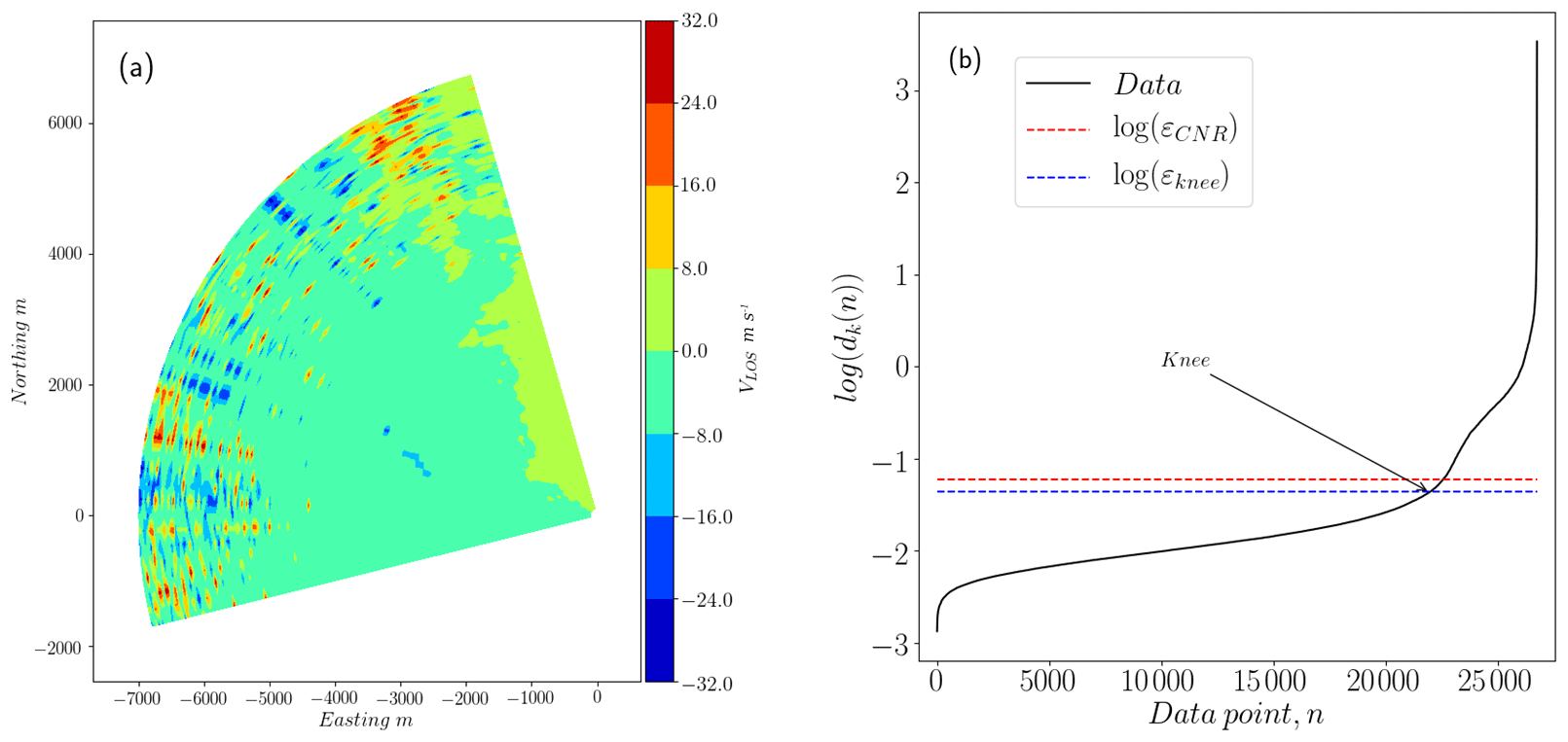
Figure 6(a) Scan from the balconies experiment (phase 1) with 48 % of data points in the range of reliable observations with CNR ∈ [−24, −8] dB. (b) Logarithm of sorted distances to the fifth-nearest neighbor for each point in a data set. The total number of observations corresponds to three consecutive scans, or 26 730 points. The sorted fifth distances show three knees separating three types of structures: reliable observations with distances below εknee, an overlapping region where the distance between points grows faster, and pure noise or nonstructured data.
The input parameters ε and NN have a significant influence on the number and characteristics of the clusters detected. For example, large ε together with a small NN will end up with sparse clusters that might include noise. In order to find the parameters separating the least dense cluster from noise, we fix NN to a certain value k and determine ε from the data density distribution. The latter is well described by the k-distance function, dk(n), which represents the distances from all data points n to their respective kth nearest neighbor, sorted in ascending order. When k is 5, for instance, d5(n) in Fig. 6 shows sudden changes (or knees) that give some indications about the data density distribution. The knee highlighted represents a limit between a group of reliable observations and the one growing fast towards noisy data. The positions of these knees in the graph correspond to the peaks in the curvature of dk(n), κ(n) in expression Eq. (3). In this expression primes correspond to the peaks in the curvature of dk(n) with respect to n. The continuous version of dk(n) is made by spline-fitting on a reduced set of uniformly distributed points over the original data set.
When scans are very noisy, the selection of a proper value of ε is difficult since knees are located closer together, and a larger fraction of observations show a fast-growing dk(n), as expected. In this case, the fraction of points showing reliable CNR values is taken into account, and ε is estimated by expression Eq. (4). Here fCNR corresponds to the fraction of observed CNR values within the range [−24, −8], and the constants c1 and c2 are obtained from the upper and lower bounds of ε in the data, respectively.
The set of features considered when filtering synthetic data does not include CNR because it is not available from the lidar simulator described in Sect. 3. For synthetic and real data sets we consider spatial location (azimuth and radial positions) and smoothness as additional features. The latter, ΔVLOS, corresponds to the median difference in VLOS between a specific position and its direct neighbors in one individual scan.
Since we consider features that vary significantly in magnitude (CNR and range gate distance for instance), we normalize the data before the application of DBSCAN. This step is necessary for the estimation of meaningful distances between observations, which is the basis of this approach. There are several
ways to do this. Here, the data in each feature are centered by subtracting their median and scaled according to their interquartile range. This aims to
minimize the influence from outliers in the normalization.
The clustering filter is implemented to be a nonsupervised classifier and does not need more input parameters than the different features and the number of scans put together as a batch before filtering. The latter is set to three in this case to speed up calculations and avoid creating clusters from noisy regions. From this point of view, this filter is also as dynamic – similar to Beck and Kühn (2017) – when applied to a real data set since it will consider the data structure within a period limited to 135 s (three scans of 45 s in our case), and characteristics of temporal evolution of the data are indirectly taken into account. For the synthetic data used in this test, more than one scan filtered per iteration gives enough data density in noisy and reliable areas of the observational space. We speculate that scans that are correlated in time will enhance the self-similarity of the data, thus improving the performance of the filter. Turbulence structures with length scales in a range between the range gate size and the scanning area size will evolve at a slower rate than the time elapsed between consecutive scans.
5.1 Synthetic data
Equations (5) to (7) define three metrics to assess the performance of the filters given prior knowledge of the position and magnitude of noise in a controlled case with N observations. The fraction of noise detected, ηnoise, quantifies the relative importance of true positives or the difference between observations identified as noise, Nnoise, and false positives, Npos, over the total number of contaminated observations. The fraction of good observations recovered, ηrecov, gives an idea of the true negatives over the total number of noncontaminated observations, Nnon-cont. True negatives are not equal to N − Nnoise since the latter might include false negatives, Nneg. The relative importance of these two metrics for a given fraction of noise in a contaminated scan, fnoise, is quantified by ηtot, which takes into account cases with a large fraction of noise detected and low recovery rate and vice versa.
5.2 Real data
In the absence of reference measurements, the quality of the data retrieved after filtering is assessed by comparing the distribution of radial wind speeds for very reliable observations (with CNR values within the range of −24 to −8 dB) with the distribution of filtered observations that fall out of this range. Observations out of the reliable range population usually show a probability density function (or PDF) with heavier tails, like the PDFs in Fig. 7. Here we understand a heavy-tailed PDF as a distribution that slowly goes to 0 and shows higher probability density for values beyond the 3σ limit (or 3 SD limit) when compared to the normal distribution, evidence of a higher probability of occurrence of outliers or extreme values. The recovering rate of observations beyond the [0.003, 0.997] quantile range of the reliable VLOS (shaded area in Fig. 7) could shed light on the quality of the data retrieved by the filter.

Figure 7Probability density function of reliable observations of VLOS (solid black line) and nonreliable observations (solid red line) for (a) phase 1 of the balconies experiment, with scans performed at 50 , and (b) phase 2 of the same campaign, with scans performed at 200
Another metric is the similarity between the PDF of reliable and nonreliable data after filtering. The distance between both probability density functions can be compared with similarity metrics like the Kolmogorov–Smirnov test (Kolmogorov, 1933) or Kullback–Leibler (KL) divergence (Kullback and Leibler, 1951). The former test measures the statistical similarity between two random variables, X1 and X2, by estimating the statistical distance, D (or K–S statistic), between their cumulative distribution functions, F1(x) and F2(x), as the supreme of their difference.
The null hypothesis here is that two realizations are from the same distribution if the K–S statistic is such that its two-tailed p-value is above a certain level α. Because the number of data analyzed here is large – we analyzed over 20 000 scans for the two phases of the Østerild campaign, each with 8910 data points, over almost 10 d – this similarity test is very precise but also very strict, rejecting the null hypothesis for small deviations between F1(x) and F2(x). Nevertheless, the K–S statistics can be used to compare which probability distribution after filtering is closer to the one representing the reliable observations.
The KL divergence is a measure of similarity or overlapping of two distributions, P1 and P2, with realizations X1 and X2, respectively. It is used in different applications to shed light on the loss of information when X1 is represented by P2 or vice versa and is defined by the expression Eq. (9).
Both metrics will be used to estimate how the distribution of nonreliable observations of VLOS is modified after filtering and if the new distribution is similar (or close in a statistical distance sense) to the probability density of reliable observations of the radial wind speed, shown in Fig. 7 for phases 1 and 2 of the measurement campaign, respectively.
Both performance metrics, the recovery rate of abnormal measurements in the tails of the PDF of reliable observations and its statistical distance to the PDF of filtered nonreliable observations, will be assessed for the median-like filter, the clustering filter, and also for data filtered with a CNR threshold of −29 dB following Gryning and Floors (2019).
6.1 Synthetic data
In Fig. 8 we can see the result of the two filters applied to one synthetic scan contaminated with procedural noise. The contaminated observations are indicated by the gray area in this scan. Extreme values contaminating VLOS are identified by both filters without problems, but subtle alterations of the original values of the scan are hard to detect for the median-like filter. The clustering filter performs very efficiently when detecting this type of contaminated observation and filters almost all the noise. Both filters repeat this behavior in all the synthetic scans used for this controlled test, as can be seen in Fig. 9, which shows the resulting metrics of the two filters applied to the whole synthetic data set. Looking at ηtot, both filters show similar mean values and spread, with the clustering filter performing slightly better. The difference becomes noticeable when we see ηnoise, which for the clustering filter shows a mean value of 0.95, far larger than the 0.67 of the median-like filter. The latter result could be problematic if the median-like filter is used since noise contaminating the filtered scan will result in nonrealistic wind fields after reconstruction.
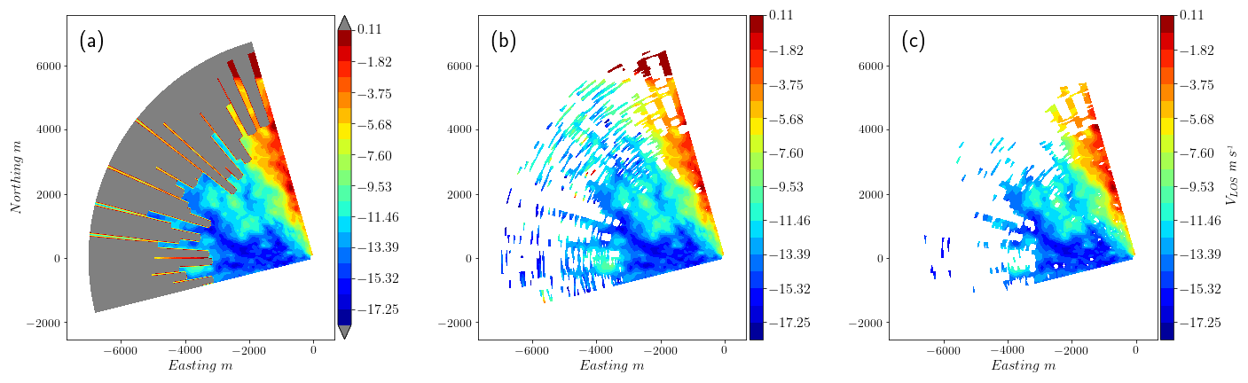
Figure 8(a) Contaminated synthetic scan with noise indicated by gray area. (b) Scan filtered using the median-like approach. (c) Clustering filter.

Figure 9Histograms of the three performance indexes for the total number of synthetic scans. (a) Both filters show similar spread, but the clustering filter rejects a rather higher fraction of noise. (b) The higher recovery rate of the median-like filter and its narrower distribution are superior to the clustering algorithm; the cost is acceptance of more contaminated observations. (c) Both filters have similar mean values for ηtot around 0.9.
Both filters perform well when evaluated in terms of ηrec, with the median-like filter showing a higher mean fraction of good observations retrieved, 0.96, compared with the 0.89 of the clustering filter. This result is expected since the median-like filter is more permissive regarding fluctuations that can seem locally anomalous for the clustering filter.
6.2 Real data
The data set from the balconies experiment presents advantages for the clustering filter since the CNR value can be included as a feature in describing the data. Nevertheless, as mentioned already in Sect. 2, we do not count on any reference to assess the performance of the filter apart from the radial wind speed distribution of very reliable observations with CNR values within the range of −24 to −8 dB. As mentioned earlier, valid observations in this range might present a similar distribution. Figure 7 shows this distribution before filtering, shadowing the area of values of VLOS that fall in the region beyond 99.7 % of the total probability or 3σ limit, usually classified as outliers. Figures 10 and 11 show the recovery fraction for CNR and median-like and clustering filters when applied to data in the reliable and nonreliable CNR ranges for phases 1 and 2 of the Østerild experiment. Unlike the clustering filter, the CNR threshold and median-like filters show nonnegligible recovery rates beyond the 3σ limit, particularly significant in the former. This result is very much in line with the ηnoise metric from the synthetic data. Within the 3σ range, the CNR and median-like filters perform slightly better than the clustering filter in terms of recovery fraction, in agreement with the results of ηrec in Sect. 6.1. Even though this might compensate the fact that CNR threshold and median-like filters fail to filter out the major part of outliers, increasing the availability of measurements, this difference does not make the PDF of the filtered data more similar to the PDF of reliable data, as Table 4 shows via the metrics DK and DKL. According to this metric, the PDF of the data after the application of the clustering approach looks more statistically similar to reliable observations. This table also shows DK and DKL of the nonreliable data before filtering, which in all cases is improved, except for DK for median and CNR threshold filters during phase 2.
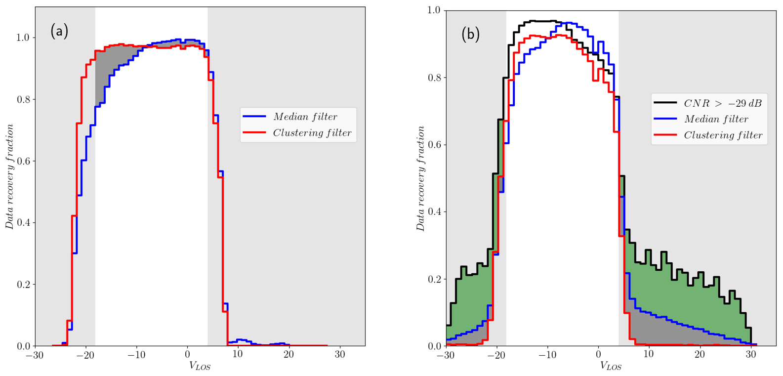
Figure 10Distribution of recovery fraction per wind speed bin for phase 1 of the experiment of (a) reliable observations (−24 < CNR < −8) and (b) nonreliable data (CNR < −24 or CNR > −8) for the three types of filters. The shadowed area in both graphs corresponds to the region where observations exceed the 99.7 % probability (or 3σ limit) in the PDF of reliable observations. The darker shadowed area highlights the additional fraction of extreme values nonfiltered by the median-like and CNR filters when the former uses the optimal input set nr = 5, nϕ = 3, and ΔVLOS, threshold = 2.33 m s−1.
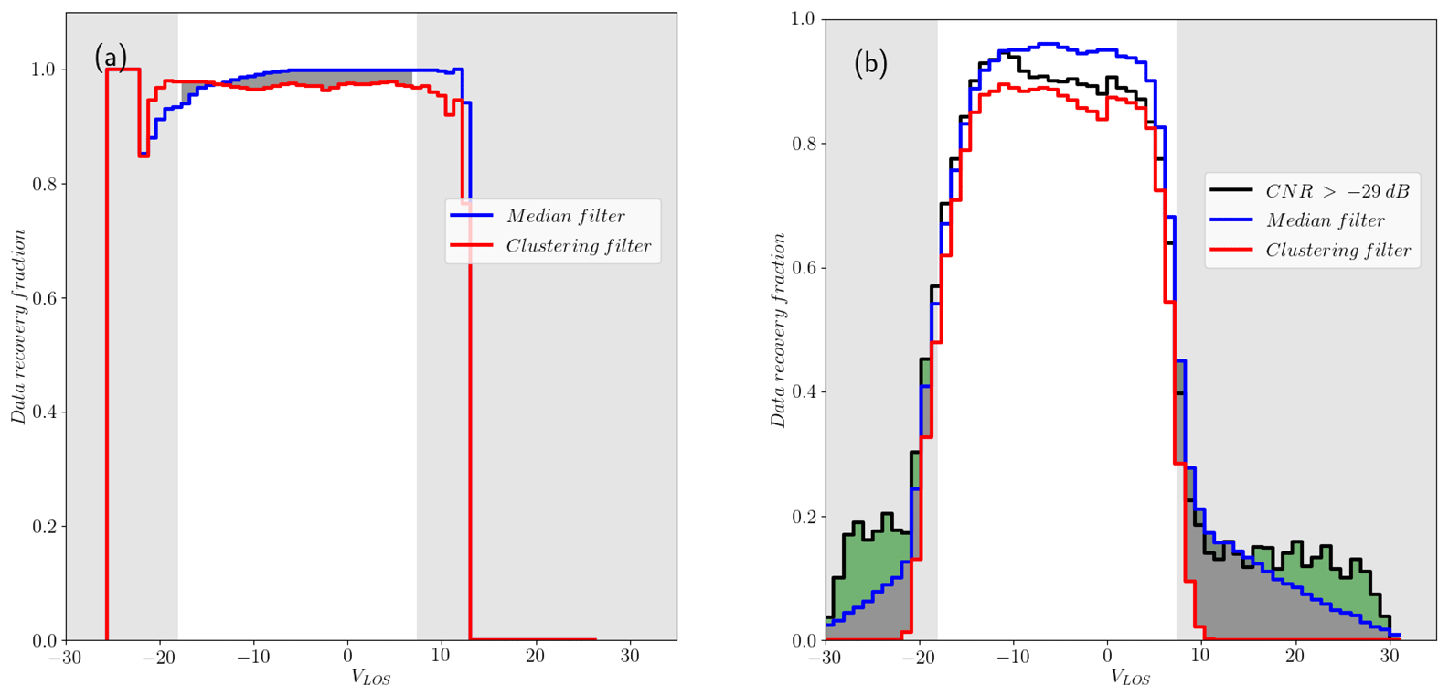
Figure 11Distribution of recovery fraction per wind speed bin for phase 1 of the experiment of (a) reliable observations and (b) nonreliable data for CNR and median and clustering filters. The shadowed area in both graphs corresponds to the region where observations exceed the 3σ limit in the PDF of reliable observations. Again, the darker shadowed area highlights the additional fraction of extreme values nonfiltered by the median-like and CNR filters when the former uses the optimal input set nr = 5, nϕ = 3 and ΔVLOS, threshold = 2.33 m s−1.
Table 4Results of PDF similarity test of reliable and nonreliable data after filtering. The CNR = −29 dB threshold is also included (Gryning and Floors, 2019).

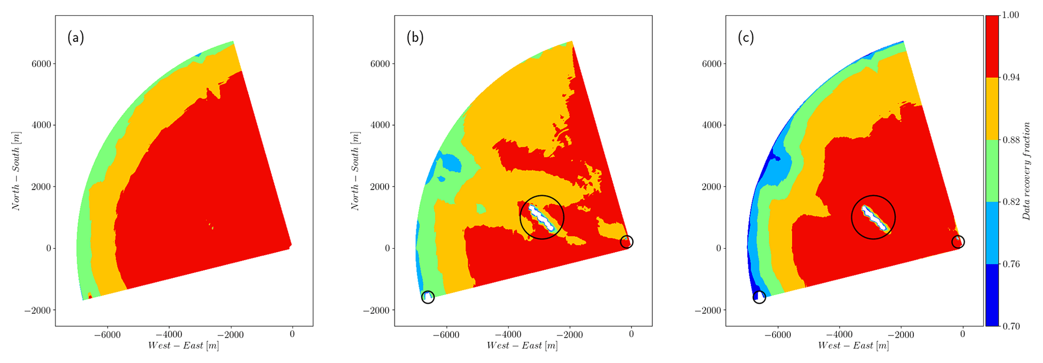
Figure 12Total recovery fraction for phase 1 of the experiment. The noisy and far regions of the scans show a high recovery, above 80 %, for (a) the CNR > −29 dB threshold filter and (b) the median-like filter and below 75 % for (c) the clustering filter. The three groups of hard targets (turbines and one meteorological mast close to the lidar), which are identified by the median and clustering filter with recovery rates below 20 %, are highlighted.
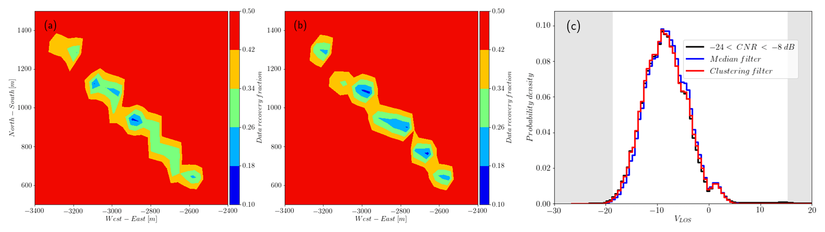
Figure 13Detail of the recovery rate at the site of the turbines for the (a) median filter and (b) clustering filter. The recovery is lower in the flow regime of the turbine cluster (there are seven turbines in line) and higher in their surroundings for the clustering filter. Red denotes recovery rates of 0.5 or higher. (c) Probability density of VLOS around the group of turbines.
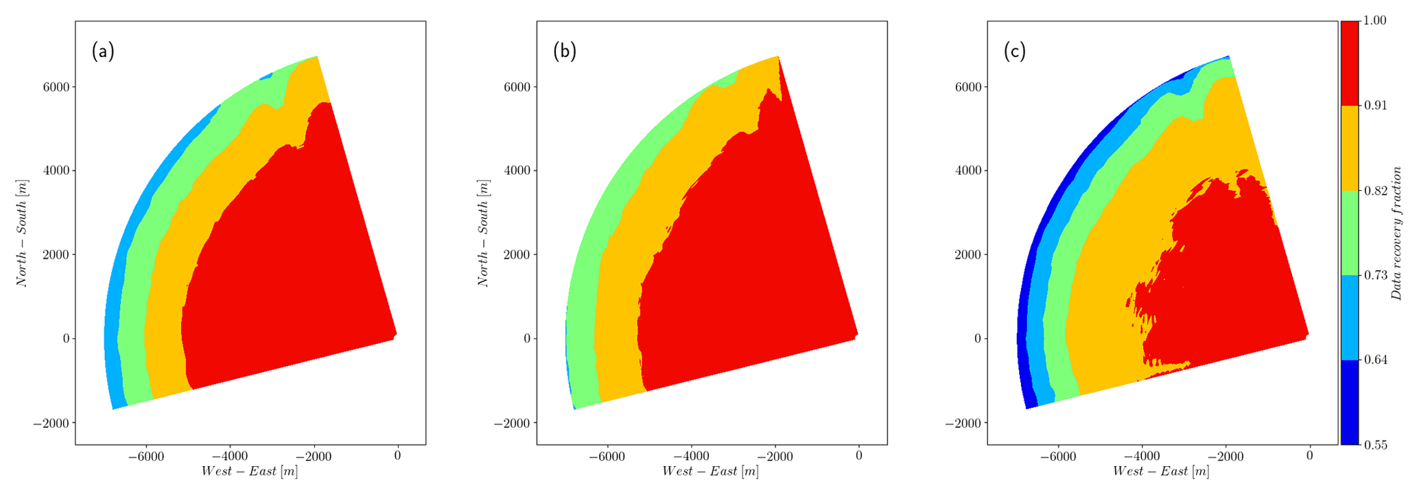
Figure 14The total recovery fraction of observations for phase 2 of the experiment. The noisy and far regions of the scans show a high recovery, above 70 %, for (a and b) the CNR > −29 dB threshold and median-like filters, respectively. The recovery decreases to 55 % in the same region for the clustering filter, in line with the previous results, assuming that outliers (above the 3σ limit) and noise are more likely to be located here.
Figures 12–14 show the performance of the three different filters in different regions of the scan from, respectively, phase 1 and 2 of the experiment. When the spatial distribution of the recovery fraction is analyzed, we can see that the lowest values shown by the clustering filter are mostly located in the far region of the scan, which in general presents low CNR values. The spatial recovery rate during phase 1 also shows that the median-like and clustering filters are able to identify hard targets, which are also a source of bad observations. For scans recorded at 50 in phase 1, backscatter is affected by a group of seven turbines located approximately in the middle of the scanning area, with one turbine touching the end of the southern beams of the scan and a meteorological mast located very close to the lidar. Figure 13 shows a detail of the recovery rate associated with the flow in the vicinity of the turbine group in which we can see that the clustering filter is able to better identify the turbine locations, recovering more data in the surroundings when compared to the median-like filter. The PDF of VLOS in this area also shows more similarities between the data filtered with the clustering algorithm and observations with CNR values in the range [−24, 8].
Table 5Additional data recovered, relative to the number of observations in the reliable range of CNR, and fraction of data recovered with values beyond the 3σ range.
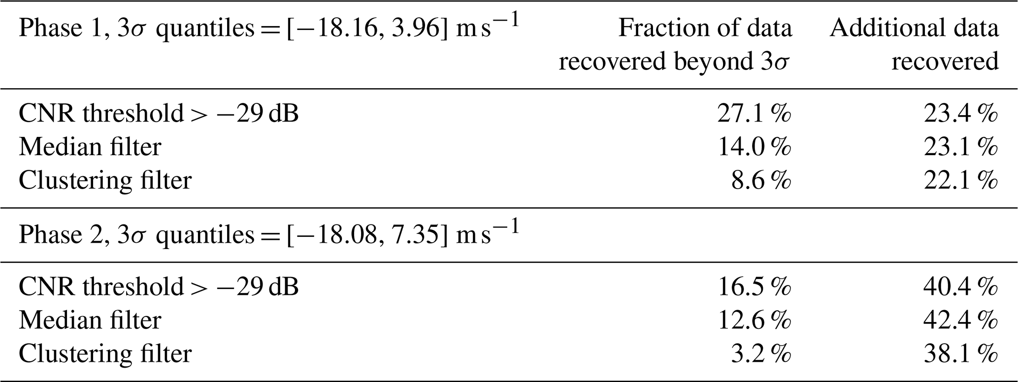
Table 5 shows a summary of the additional data available when the CNR = −29 dB threshold and the median-like and clustering filters are applied instead of the more conservative and restrictive CNR = −24 dB threshold filter. Additionally, this table shows the fraction of observations exceeding the 3σ limit that are recovered by the three filters. Even though the clustering filter shows a slightly lower fraction of additional data available when compared to the other filters, most of it comes from values within the 3σ region. Moreover the quality of the data recovered by the clustering approach seems to be higher when all these results are tested with the performance metrics defined in Sect. 5.
The metrics introduced in Sect. 5.1 attempt to evaluate two different capabilities of the filters: the quality and number of data recovered. In general these two metrics are in conflict every time a high rate of noise detection will decrease the data recovery. The metric ηtot attempts to quantify their relative importance regarding the noise fraction, which in this study is distributed in a relatively wide range but on average represents 20 % of the total number of measurements per scan. The impact of the noise fraction distribution on the performance of the filters was not explored, and variations in its dispersion and mean value might be necessary. Regarding the synthetic scans, they do not allow the identification of outliers in the time domain because they are time-independent. Time-evolving synthetic turbulence fields would be necessary to generate scans correlated in time and enhance the self-similarity of the data. This might improve the performance of the clustering approach and allow the addition of a time dependence in the median-like filter, used already in Meyer Forsting and Troldborg (2016).
The synthetic wind fields used here do not consider the presence of hard targets. These anomalies in the wind field are observed by lidars as points with high CNR values and abnormal VLOS. Assessing the performance of the filters in detecting such anomalies needs a more realistic model of the pulsed lidar. This lidar simulator would allow the generation of information normally available in real lidar measurements, like CNR, and the spread in the power spectra of the heterodyne signal, Sb. This additional information will benefit the performance assessment of the clustering filter and the simulation of hard targets. A more realistic lidar model was already implemented by Brousmiche et al. (2007), which can be used to further explore these aspects of the filtering process.
The data set analyzed from the balconies experiment corresponds to horizontal scans at 50 and 200 , limiting the analysis to one scanning pattern. Different scanning patterns in vertical and horizontal planes as well as wind fields over different topography would make this analysis more general, thus shedding light on the capabilities of the filters presented here. This is especially critical regarding the median-like filter, which might require again a sensitivity analysis to select proper parameters that adapt to different scanning patterns and turbulence field characteristics. So far, ΔVLOS, threshold showed a dependence on the L and αε2∕3 parameters during the sensitivity analysis presented in Sect. 6.1. Larger fluctuations in the VLOS field, whether they come from larger turbulent structures, higher turbulence energy, or both, will need a larger value of ΔVLOS, threshold to avoid the rejection of good measurements. Range height indicator (RHI) scanning patterns can pose the challenge of strong vertical shear and small turbulent structures that will need to reduce the window size nr and nϕ for the median-like filter and the selection of a different set of features (or a new definition for ΔVLOS) for the clustering filter in order to keep reliable observations from being filtered out.
Regarding feature selection, the clustering filter could consider the spectral spreading of the heterodyne signal, Sb, and time variation of VLOS in addition to features already used in this work to characterize and distinguish better clustering of good measurements. Nevertheless, due to the Euclidean distance definition, additional dimensions will make the data more sparse in higher dimensions, making it necessary to use more data points per filtering step (here we used only three scans at a time) to avoid the identification of good observations as spread-out, low-density noise. It is because of this that the application of a feature selection method might be necessary (Chandrashekar and Sahin, 2014).
Using the statistical distances DK and DKL as a metric for the filter performance might not be totally correct. At range gates far from the lidar, the distance between beams increases as well as the area covered by the accumulation of spectral information in the azimuth direction. Averaging VLOS over larger areas as we move forward through each beam might affect the statistics and the PDF of VLOS (especially its spread) in the outer region of the scan. The fact that this region is where we usually find the nonreliable measurement group may make the PDFs of reliable and nonreliable observations somewhat different. These possible deviations need to be investigated further.
The selection of features and the number of scans put together per filtering step or iteration could also be automated using feature selection
methods. Nevertheless, this would make the clustering filter more complex in its implementation and more computationally expensive, which is the main
disadvantage of this approach compared to the median-like filter. Very efficient median filters can achieve a computational complexity up to
𝒪(n), with n being the number of observations in the data set. Depending on the data structure, DBSCAN shows a computational complexity
from 𝒪(nlog (n)) to 𝒪(n2). If the distance between points is in general smaller than ε, the first limit can be
achieved, but clusters with different densities makes the algorithm less efficient. In the data analyzed here, having clusters with different
densities is not an issue. Nevertheless, for nonhomogeneous flows, scans might persistently show regions with VLOS, CNR, or other features
with noticeably different values. It may then be necessary to revisit the clustering algorithm used and implement an ε-independent clustering approach,
like OPTICS (Ankerst et al., 1999) for instance.
The CNR threshold filtering has been the common approach to retrieve reliable observations from lidar measurements. In this work we compared this approach against two alternative techniques: a median-like filter based on the assumption of smoothness of the wind field, hence in the smoothness of the radial wind speed observed by a wind lidar, and a clustering filter based on the assumption of self-similarity of the observations captured by the wind lidar and the possibility of clustering them in groups of good data and noise. A controlled test was carried out on the last two approaches using a simple lidar simulator that sampled scans from synthetic wind fields later contaminated with procedural noise. The results indicate that the clustering filter is capable of detecting more added noise than the median-like filter at a good recovery rate of noncontaminated data. When the three filters are tested on real data, the clustering approach shows a better performance when identifying abnormal observations, increasing the data availability between 22 % and 38 % and reducing the recovery of abnormal measurements between 70 % and 80 % when compared to a CNR threshold. This is an important result because it increases the spatial coverage of the data which can be used later for wind field reconstruction and wind data analysis, especially in the far region of the scan, which covers the largest measured area.
Even though the median-like filter is computationally efficient, it needs an optimal definition of input parameters, which are dependent on the turbulence characteristics of the wind field. The clustering filter is more robust in this sense because it is capable of automatically adapting its parameters to the structure of the data. This is a step forward to a more robust and automated processing of data from lidars, which ideally should be independent of the turbulence characteristics of the measured wind field or the scanning pattern used.
Figure A1 shows contours that present the optimal value for ηtot among all possible values of ΔVLOS, threshold and nϕ for nr = 5, the optimal window size in the radial direction. Large ΔVLOS, threshold results in large ηrecov but poor results for ηnoise and the opposite for values of the threshold, as expected. The metric ηtot then becomes relevant to determine the optimal combination of parameters. From the contours it is possible to see that the performance in terms of the ηtot metric is less sensitive to nϕ than ΔVLOS, threshold. Even though the results here show average metrics for all the scans simulated, the optimal value of ΔVLOS, threshold increases with the turbulence energy and length scale parameters, which is problematic because it requires previous knowledge of turbulence characteristics that usually are not available before reconstruction and, more importantly, data filtering.
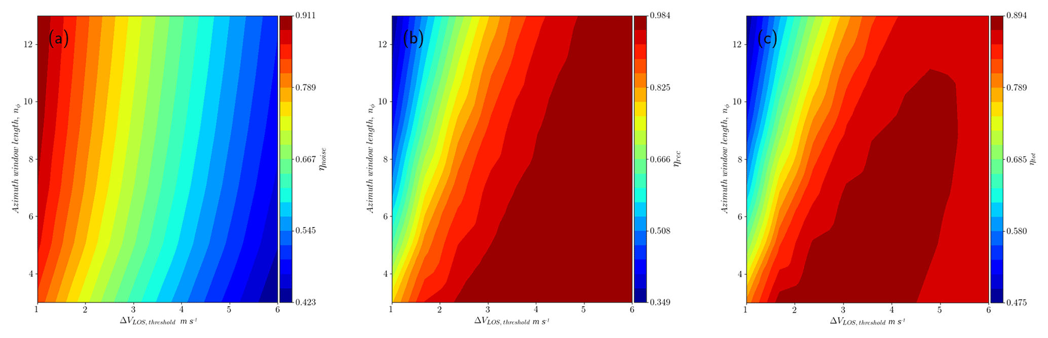
Figure A1Contours of performance metrics for nr = 5 over the ΔVLOS, threshold-nϕ space. Each point in the contour plot corresponds to the mean value of (a) ηnoise, (b) ηrec and (c) ηtot among all the 4305 synthetic scans filtered. The optimal value corresponds to nr = 5, nϕ = 3, and ΔVLOS, threshold = 2.33 m s−1.
The synthetic data and code are available at https://doi.org/10.5281/zenodo.4014151 (Alcayaga, 2020). Real data can be found at https://doi.org/10.11583/DTU.7306802.v1 (Simon and Vasiljevic, 2018).
LA implemented the analysis on synthetic and real data and wrote all sections of this paper.
The author declares that there is no conflict of interest.
I would like to thank Ioanna Karagali for comments and guidance through the data from the Østerild balconies experiments; Robert Menke for the first version of the median-like filter; and Ebba Dellwik, Nikola Vasiljevic, Gunner Larsen, Mark Kelly, and Jakob Mann for the very useful and clarifying feedback during the analysis and writing process.
This paper was edited by Murray Hamilton and reviewed by two anonymous referees.
Alcayaga, L.: Lidar data filtering algorithms, Zenodo, https://doi.org/10.5281/zenodo.4014151, 2020. a
Ankerst, M., Breunig, M. M., Kriegel, H.-P., and Sander, J.: OPTICS: Ordering Points To Identify the Clustering Structure, in: Proc. ACM SIGMOD'99 Int. Conf. on Management of Data, 1–3 June 1999, Philadelphia, Pennsylvania, USA, pp. 49–60, ACM Press, 1999. a
Backer, E.: Computer-assisted Reasoning in Cluster Analysis, Prentice Hall International (UK) Ltd., Hertfordshire, UK, 1995. a
Banakh, V. A. and Smalikho, I. N.: Estimation of the Turbulence Energy Dissipation Rate from the Pulsed Doppler Lidar Data, Atmos. Ocean. Opt., 10, 957–965, 1997. a
Beck, H. and Kühn, M.: Dynamic Data Filtering of Long-Range Doppler LiDAR Wind Speed Measurement, Remote Sens., 9, 561, https://doi.org/10.3390/rs9060561, 2017. a, b
Brousmiche, S., Bricteux, L., Sobieski, P., Macq, B., and Winckelmans, G.: Numerical simulation of a heterodyne Doppler LIDAR for wind measurement in a turbulent atmospheric boundary layer, in: 2007 IEEE International Geoscience and Remote Sensing Symposium, 23–27 July 2007, Barcelona, Spain, https://doi.org/10.1109/IGARSS.2007.4423420, 2007. a
Burger, W. and Burge, M. J.: Digital Image Processing – An Algorithmic Introduction using Java, Texts in Computer Science, Springer, London, UK, 2008. a
Cariou, J.: Remote Sensing for Wind Energy, chap. Pulsed lidars, DTU Wind Energy, Denmark, 131–148, 2015. a, b
Chandrashekar, G. and Sahin, F.: A Survey on Feature Selection Methods, Comput. Electr. Eng., 40, 16–28, https://doi.org/10.1016/j.compeleceng.2013.11.024, 2014. a
Ester, M., Kriegel, H.-P., Sander, J., and Xu, X.: A Density-based Algorithm for Discovering Clusters a Density-based Algorithm for Discovering Clusters in Large Spatial Databases with Noise, in: Proceedings of the Second International Conference on Knowledge Discovery and Data Mining, KDD'96, 2–4 August 1996, Portland, Oregon, 226–231, 1996. a
Gryning, S. and Floors, R.: Carrier-to-Noise-Threshold Filtering on Off-Shore Wind Lidar Measurements, Sensors, 19, 592, https://doi.org/10.3390/s19030592, 2019. a, b, c
Gryning, S., Floors, R., Peña, A., Batchvarova, E., and Brümmer, B.: Weibull Wind-Speed Distribution Parameters Derived from a Combination of Wind-Lidar and Tall-Mast Measurements Over Land, Coastal and Marine Sites, Bound-Lay. Meteorol., 159, 329, https://doi.org/10.1007/s10546-015-0113-x, 2016. a
Huang, T., Yang, G., and Tang, G.: A fast two-dimensional median filtering algorithm, IEEE T. Acoust. Speech, 27, 13–18, https://doi.org/10.1109/TASSP.1979.1163188, 1979. a, b
Karagali, I., Mann, J., Dellwik, E., and Vasiljević, N.: New European Wind Atlas: The Østerild balconies experiment, J. Phys. Conf. Ser., 1037, 052029, https://doi.org/10.1088/1742-6596/1037/5/052029, 2018. a, b, c, d, e
Kolmogorov, A.: Sulla determinazione empirica di una lgge di distribuzione, Inst. Ital. Attuari, Giorn., 4, 83–91, https://ci.nii.ac.jp/naid/10010480527/en/ (last access: 4 September 2020), 1933. a
Kullback, S. and Leibler, R. A.: On Information and Sufficiency, Ann. Math. Stat., 22, 79–86, 1951. a
MacQueen, J.: Some methods for classification and analysis of multivariate observations, in: Proceedings Fifth Berkeley Symp. on Math. Statist. and Prob., vol. 1: Statistics, 21 June–18 July 1965 and 27 December 1965–7 January 1966, Berkeley, California, USA, 281–297, 1967. a
Mandelbrot, B.: The fractal geometry of nature, W. H. Freeman and Comp., New York, USA, 1983. a
Mann, J.: The spatial structure of neutral atmospheric surface-layer turbulence, J. Fluid Mech., 273, 141–168, https://doi.org/10.1017/S0022112094001886, 1994. a
Mann, J.: Wind field simulation, Probabilist. Eng. Mech., 13, 269–282, https://doi.org/10.1016/S0266-8920(97)00036-2, 1998. a, b
Mann, J., Angelou, N., Arnqvist, J., Callies, D., Cantero, E., Arroyo, R. C., Courtney, M., Cuxart, J., Dellwik, E., Gottschall, J., Ivanell, S., Kühn, P., Lea, G., Matos, J. C., Palma, J. M. L. M., Pauscher, L., Peña, A., Sanz, R. J., Söderberg, S., Vasiljevic, N., and Veiga, R. C.: Complex terrain experiments in the new european wind atlas, Philos. T. R. Soc. A, 375, 20160101, https://doi.org/10.1098/rsta.2016.0101, 2017. a
Menke, R., Vasiljević, N., Wagner, J., Oncley, S. P., and Mann, J.: Multi-lidar wind resource mapping in complex terrain, Wind Energ. Sci., 5, 1059–1073, https://doi.org/10.5194/wes-5-1059-2020, 2020. a
Meyer Forsting, A. and Troldborg, N.: A finite difference approach to despiking in-stationary velocity data - tested on a triple-lidar, J. Phys. Conf. Ser., 753, 072017, https://doi.org/10.1088/1742-6596/753/7/072017, 2016. a, b, c
Pedregosa, F., Varoquaux, G., Gramfort, A., Michel, V., Thirion, B., Grisel, O., Blondel, M., Prettenhofer, P., Weiss, R., Dubourg, V., Vanderplas, J., Passos, A., Cournapeau, D., Brucher, M., Perrot, M., and Duchesnay, E.: Scikit-learn: Machine Learning in Python, J. Mach. Learn. Res., 12, 2825–2830, 2011. a
Perlin, K.: Noise hardware, in: Real-Time Shading SIGGRAPH, Course Notes, Baltimore, Maryland, USA, 2001. a, b
Simon, E. and Vasiljevic, N.: Østerild Balconies Experiment (Phase 2), figshare, https://doi.org/10.11583/DTU.7306802.v1, 2018. a, b, c, d
Smalikho, I. N. and Banakh, V. A.: Accuracy of estimation of the turbulent energy dissipation rate from wind measurements with a conically scanning pulsed coherent Doppler lidar. Part I. Algorithm of data processing, Atmos. Ocean. Opt., 26, 404–410, https://doi.org/10.1134/S102485601305014X, 2013. a
Stawiarski, C., Träumner, K., Knigge, C., and Calhoun, R.: Scopes and Challenges of Dual-Doppler Lidar Wind Measurements – An Error Analysis, J. Atmos. Ocean. Tech., 30, 2044–2062, https://doi.org/10.1175/JTECH-D-12-00244.1, 2013. a
Vasiljević, N., Lea, G., Courtney, M., Cariou, J., Mann, J., and Mikkelsen, T.: Long-Range WindScanner System, Remote Sens., 8, 896, https://doi.org/10.3390/rs8110896, 2016. a, b, c, d
Vasiljević, N., L. M. Palma, J. M., Angelou, N., Carlos Matos, J., Menke, R., Lea, G., Mann, J., Courtney, M., Frölen Ribeiro, L., and M. G. C. Gomes, V. M.: Perdigão 2015: methodology for atmospheric multi-Doppler lidar experiments, Atmos. Meas. Tech., 10, 3463–3483, https://doi.org/10.5194/amt-10-3463-2017, 2017. a
- Abstract
- Introduction
- Real data: Østerild balconies experiment
- Synthetic data
- Filtering techniques applied on real and synthetic data
- Performance metrics
- Results
- Discussion
- Conclusions
- Appendix A: Sensitivity analysis on median-like filter parameters
- Code and data availability
- Author contributions
- Competing interests
- Acknowledgements
- Review statement
- References