the Creative Commons Attribution 4.0 License.
the Creative Commons Attribution 4.0 License.
 | 01 Dec 2020
Interpolation uncertainty of atmospheric temperature profiles
Alessandro Fassò
Michael Sommer
Christoph von Rohden
This paper is motivated by the fact that, although temperature readings made by Vaisala RS41 radiosondes at GRUAN sites (https://www.gruan.org/, last access: 30 November 2020) are given at 1 s resolution, for various reasons, missing data are spread along the atmospheric profile. Such a problem is quite common with radiosonde data and other profile data. Hence, (linear) interpolation is often used to fill the gaps in published data products. From this perspective, the present paper considers interpolation uncertainty, using a statistical approach to understand the consequences of substituting missing data with interpolated data.
In particular, a general framework for the computation of interpolation uncertainty based on a Gaussian process (GP) set-up is developed. Using the GP characteristics, a simple formula for computing the linear interpolation standard error is given. Moreover, the GP interpolation is proposed as it provides an alternative interpolation method with its standard error.
For the Vaisala RS41, the two approaches are shown to provide similar interpolation performances using an extensive cross-validation approach based on the block-bootstrap technique. Statistical results about interpolation uncertainty at various GRUAN sites and for various missing gap lengths are provided. Since both approaches result in an underestimation of the interpolation uncertainty, a bootstrap-based correction formula is proposed.
Using the root mean square error, it is found that, for short gaps, with an average length of 5 s, the average uncertainty is less than 0.10 K. For larger gaps, it increases up to 0.35 K for an average gap length of 30 s and up to 0.58 K for a gap of 60 s. It is concluded that this approach could be implemented in a future version of the GRUAN data processing.
- Article
(4434 KB) - Full-text XML
- BibTeX
- EndNote


The quality of climate variable profiles in the atmosphere is relevant in various scientific fields. In particular, it is important for numerical weather prediction, satellite observation validation, and climate change understanding, including extreme events such as droughts and tornadoes. In this framework, more than 10 years ago, the GCOS (Global Climate Observing System) Reference Upper-Air Network (GRUAN, https://www.gruan.org/) was established to provide reference measurements from the surface, through the troposphere, and into the stratosphere (Seidel et al., 2009; Bodeker et al., 2016). Immler et al. (2010) discussed the concepts of reference measurements, traceability, full metadata description, a proper manufacturer-independent instrument characterisation, and the assessment of measurement uncertainties for upper-air observations.
GRUAN data processing for the Vaisala RS92 radiosonde was developed to meet the above criteria for reference measurements (Dirksen et al., 2014). The related data product is characterised not only by the above-mentioned metrological requirements, but also by high vertical resolution. After the introduction of the new Vaisala RS41 radiosonde, GRUAN is currently developing the corresponding data processing for the new instrument (Dirksen et al., 2020).
Although temperature readings made by the Vaisala RS41 radiosonde at GRUAN sites are given at 1 s resolution, for various reasons, missing data are sometimes present along the atmospheric profile. If interpolation is applied to fill in the missing values, the uncertainty introduced through interpolation should be considered in the uncertainty budget.
The literature has considered the interpolation of atmospheric profiles from various points of view. In some cases, interpolation is applied to measurement uncertainty. For example, considering the AERONET Version 3 aerosol retrievals, Sinyuk et al. (2020) obtained the uncertainty by interpolation of a lookup table.
A second and more relevant use of interpolation relates to the measurement itself. In this field, Ceccherini et al. (2018) used interpolation for the data fusion of ozone satellite vertical profiles. Interpolation uncertainty and, more generally, co-location uncertainty have been computed using simulated profiles. Similarly, for co-location uncertainty of the total ozone, Verhoelst et al. (2015) used interpolation in the so-called OSSSMOSE simulator.
In the framework of radiosonde co-location uncertainty, considering relative humidity, Fassò et al. (2014) used a statistical approach based on the heteroskedastic functional regression model. Considering pressure, Ignaccolo et al. (2015) extended the latter approach to three-dimensional functional regression. In these two papers, interpolation uncertainty is implicitly assessed by means of model error variance.
Comparisons of radiosonde and satellite data are sometimes based on low-vertical-resolution radiosonde profiles, especially for historical data. In some cases, interpolation is not required because of the higher vertical resolution of satellite profiles (Sun et al., 2010). In other cases, interpolation is required. For example, Finazzi et al. (2019) considered the harmonisation of low-vertical-resolution temperature and humidity radiosonde measurements and the corresponding atmospheric profiles derived from the Infrared Atmospheric Sounding Interferometer (IASI) aboard the Metop-A and Metop-B satellites. These authors used spline interpolation of radiosonde profiles and indirectly assessed the related uncertainty through a comparison with GRUAN reference measurements.
As a common trait of the above literature, interpolation of atmospheric profiles is quite common, but a systematic analysis of interpolation uncertainty per se is not yet available. A general approach to interpolation is the geostatistics approach (Cressie and Wikle, 2011), which is similar to the Gaussian process (GP) approach (Rasmussen and Williams, 2006). Its value is due to the fact that it gives optimal interpolation under some conditions. With some variations, the related optimal interpolation algorithm is based on the autocovariance function or, equivalently, on the structure function (Sofieva et al., 2008). This approach is often used to interpolate in spaces of increasing complexity, such as the Euclidean plane, the sphere (Alegria et al., 2017), the three-dimensional Euclidean space, or the circular shell representing the atmosphere (Porcu et al., 2016). Interestingly, it can be shown that the spline interpolation is a special case of the GP interpolation (Kimeldorf and Wahba, 1970). Another interesting point is that the GP approach comes with a formula for interpolation uncertainty estimation. It must be noted that the formula is correctly used if the true data generation mechanism is a GP. If the GP is simply an approximation, an additional term must be added.
In this paper, the uncertainty of the one-dimensional linear interpolation is discussed using two approaches. In the first stage, the closed-form formula of the linear interpolation uncertainty is presented under the assumption that the observed atmospheric profile is generated by a GP. In the second stage, thanks to the availability of good profiles without missing data, the GP assumption is relaxed, and a block-bootstrap correction of the uncertainty formula is constructed. This approach is valid for any atmospheric profile data set. Considering the motivating application, which focuses on temperature readings of the Vaisala RS41 at GRUAN sites, this paper's objective is to contribute to the understanding of interpolation uncertainty expressed as a function of missing gap length, missing frequency, altitude, and site. This objective amounts to studying the feasibility of an algorithm and/or a lookup table providing interpolation uncertainty in a future version of GRUAN data processing.
To achieve this objective, each good profile is divided into a learning set and a testing set. Firstly, data from the testing set are considered missing and are estimated by interpolation of the learning set data. Secondly, the comparison of estimated and true data in the testing set is used for interpolation uncertainty assessment. This assessment is done for various missing patterns that resemble observed bad launches, which are characterised by many missing measurements. In particular, increasing gap average lengths will be analysed. The testing sets will be extracted using a block-bootstrap approach (Politis and Romano, 1994; Mudelsee, 2014). Hence, although the numerical results are specific to the Vaisala RS41 temperature data set, the approach is quite general and may be applied to other sensors.
The rest of the paper is organised as follows. Section 2 motivates the paper by discussing the sources of gaps in data reception and their impact in GRUAN data processing. Section 3 introduces the GP set-up used to provide the formal assessment of linear interpolation uncertainty and to introduce the GP interpolation with its standard deviation. Section 4 presents the data sets, which are related to Vaisala RS41 observations at seven GRUAN sites and are used in the empirical analysis. Section 5 describes the re-sampling technique able to simulate random patterns of missing values of different durations. Section 6 describes the cross-validation scheme essential for the uncertainty computations and the model selection, which is discussed in Sect. 7. Section 8 presents the results, compares the behaviour of the two interpolation techniques, and proposes an empirically corrected formula for interpolation uncertainty. Finally, Sect. 9 draws some conclusions.
There are several possible reasons for temporary gaps in data reception. These include the presence of obstacles that may interfere with radio transmission to the ground site (trees, buildings, local geography), extraordinary meteorological conditions, or instrument-related reasons. Considering an ascent as a trajectory, rather than a vertical profile, the probability of data gap occurrence increases with the horizontal distance from the launch site (weaker radio signal), which can significantly exceed the vertical distance, depending on wind conditions.
A preliminary statistical analysis of the occurrence of data gaps in RS41 radiosonde soundings performed at 15 GRUAN stations in the 2014–2019 period shows that gaps occur in more than 20 % of the soundings, virtually independently of the height ranges, with the majority (>95 %) having fewer than 15 gaps per 1000 s. Up to 30 km, gaps >10 s only play a role in about 5 % of the ascents; however, the occurrence of larger gaps generally increases with height (distance). Figure 1 gives an example of the stratospheric height section between 20 and 25 km, where 13 667 profiles are included.
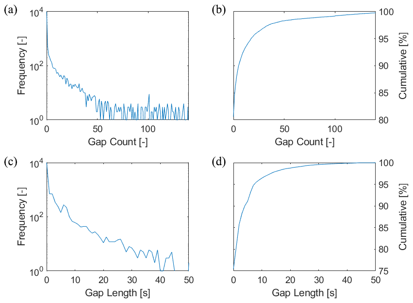
Figure 1Frequency distribution of temperature gaps in the stratospheric height section between 20 and 25 km, based on 13 667 RS41 profiles, years 2014–2019. (a) Frequency distribution of the number of data gaps (independent of gap length). (c) Frequency distribution of the length of the largest gap identified in a profile. Panels (b) and (d) show the corresponding cumulative frequencies.
The GRUAN data processing is based on the raw data from the physical radiosonde sensors, namely temperature, relative humidity, positioning data provided by the Global Navigation Satellite System (GNSS), and pressure if an onboard sensor is present. The raw data are corrected for known or experimentally evidenced systematic effects, such as adjustments from pre-flight ground checks, corrections of sensor time lags, or solar radiative effects. Some intermediate variables are, in turn, calculated (e.g. effective air speed or ventilation) as components of the correction algorithms. A number of secondary variables are finally derived, for example, altitude, geopotential height, water vapour content, or wind components. At different processing stages, smoothing filters are applied for estimation and separation of the signal's noise components. Through all these steps, the regular grid of the measured raw data is maintained; that is, all variables and uncertainties in the product variables are given with the original high resolution.
This procedure inevitably leads to specific technical difficulties if data gaps occur randomly or intermittently. For example, smoothing may introduce effects which are difficult to handle when running over gaps, especially for gap sizes comparable to or exceeding the actual kernel length. The same difficulty applies to uncertainty estimates to be associated with the averaged (smoothed) values. Another example is related to magnitudes which are calculated cumulatively with height, such as pressure derived from positioning, temperature, and humidity data, or the integrated water vapour content. As a consequence, processing-related irregularities or deviations may occur in the profile data and uncertainty estimates, the systematics and extent of which are difficult to predict. Depending on the purpose for which the GRUAN data product is further used (e.g. process studies based on high-resolution data or average-based long-term studies for climate), such systematics may have a different impact.
In this section, formulas of the uncertainty for both linear and stochastic interpolation are considered under some stochastic assumptions about the data generation mechanism.
In particular, considering a radiosonde flight, we assume that is the flying time in seconds from take-off and y(t) is the observed temperature in Kelvin, provided by the following measurement error equation:
In Eq. (1), s(t) is the unobserved true temperature and ϵ(t) is the zero mean measurement error. In each atmospheric layer, the former is assumed to follow a GP, characterised by a power exponential autocovariance function (Cressie and Wikle, 2011; Rasmussen and Williams, 2006), and the latter is assumed to follow a white noise GP. Hence, conditional on some unobserved time-dependent atmospheric conditions denoted by a(t), the GP y(t) has the following autocovariance function:
where p=1, 2, the dependence on a(t) is omitted on the right-hand side for notational simplicity, and I is the indicator function; that is, I=1 if and zero else. It is worth observing that the model in Eq. (2) is an important subset of the Matérn class, which is extensively used in statistics, machine learning and atmospheric sciences (Genton, 2001). For p=2, the unobserved true temperature has very smooth paths, since the corresponding GP has infinitely differentiable trajectories, while for p=1, the differentiability condition does not hold, and the correlation decreases faster at short distances.
From Eq. (2), the (conditional) variance of y(t) is given by
where σs>0 is the standard error of s(t) and σϵ≥0 is the measurement uncertainty, i.e. . For the instruments installed on the Vaisala RS41, it is known that the sensor-intrinsic noise of a temperature sensor is very minimal (<0.01 K), hence we expect to find a small σϵ for the data of this paper. In addition, θ>0 represents the atmospheric persistence range.
The GP is characterised by the parameter set , which is assumed to be slowly varying in time, hence characterising locally the atmospheric conditions a(t):
Note that, from the practical point of view, the random error ϵ is a Gaussian white noise and σϵ represents the random uncertainty, while (vertically) correlated errors could be confused with s(t). This point will be considered further in Sect. 8.
3.1 Linear interpolation
Considering an observation gap in the interval , the linear interpolation at time t, with t in the gap interval , is straightforwardly defined by the following formula:
where and . In general, the interpolation uncertainty u(t) is based on the expected value of the squared interpolation error, namely
Clearly, it is defined in terms of the true signal s(t) and is related to the interpolation mean square error, , by the well-known relation
Since the measurement uncertainty σϵ is unknown in our case, estimating u(t) directly from the data is an issue, and a statistical modelling approach is needed.
Assuming that the true signal s is a GP, as discussed above, the Appendix shows that the linear interpolation uncertainty given in Eq. (6) may be computed by the following standard error (SE) formula:
where, with abuse of notation, α=α(t). Note that SE(t)2=u(t)2 if the GP assumption is satisfied, but two different symbols are used because, in Sect. 8, this assumption will be relaxed.
Equation (8) defines a function of t which depends on the atmospheric persistence modelled by γ and the gap size . Since γ is not continuous in zero, the same happens to SE(t) at the gap interval borders.
Figure 2 considers the case where s(t) is a white noise – that is, γ(h)=0 for h≠0 and . At the gap borders, the interpolation is error-free, , and the uncertainty is . For t strictly inside the gap interval, we have
where the minimum is achieved in the centre of the gap interval. In this particular case, the uncertainty range does not depend on the gap size.
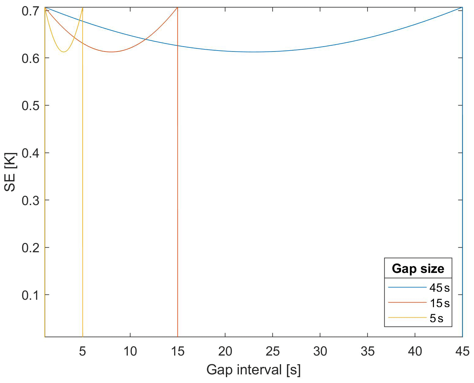
Figure 2Linear interpolation standard error (SE), Eq. (8), as a function of the gap time for a white noise process with σs=0.5 K and σϵ=0.01 K. Three gap sizes are considered: 45, 15, and 5 s.
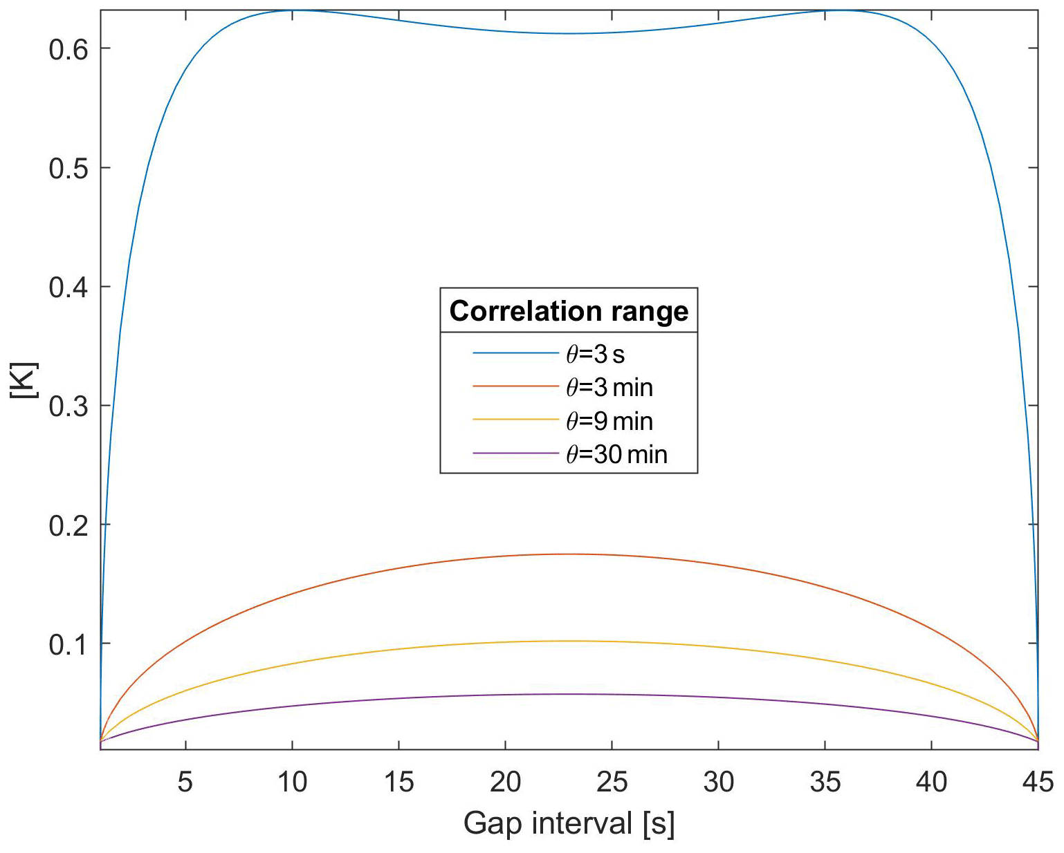
The above thresholds may be overcome in the presence of correlation. In general, for a GP with θ>0, the uncertainty depends both on the GP characteristics and the gap size. As an illustration, using σs=0.5 K, σϵ=0.01 K, and θ=3 s, Fig. 3 shows how the interpolation uncertainty depends on the gap size and on the distance from the observations in the presence of a short correlation range. More interestingly for applications, Fig. 4 shows that the linear interpolation uncertainty strongly depends on the correlation range.
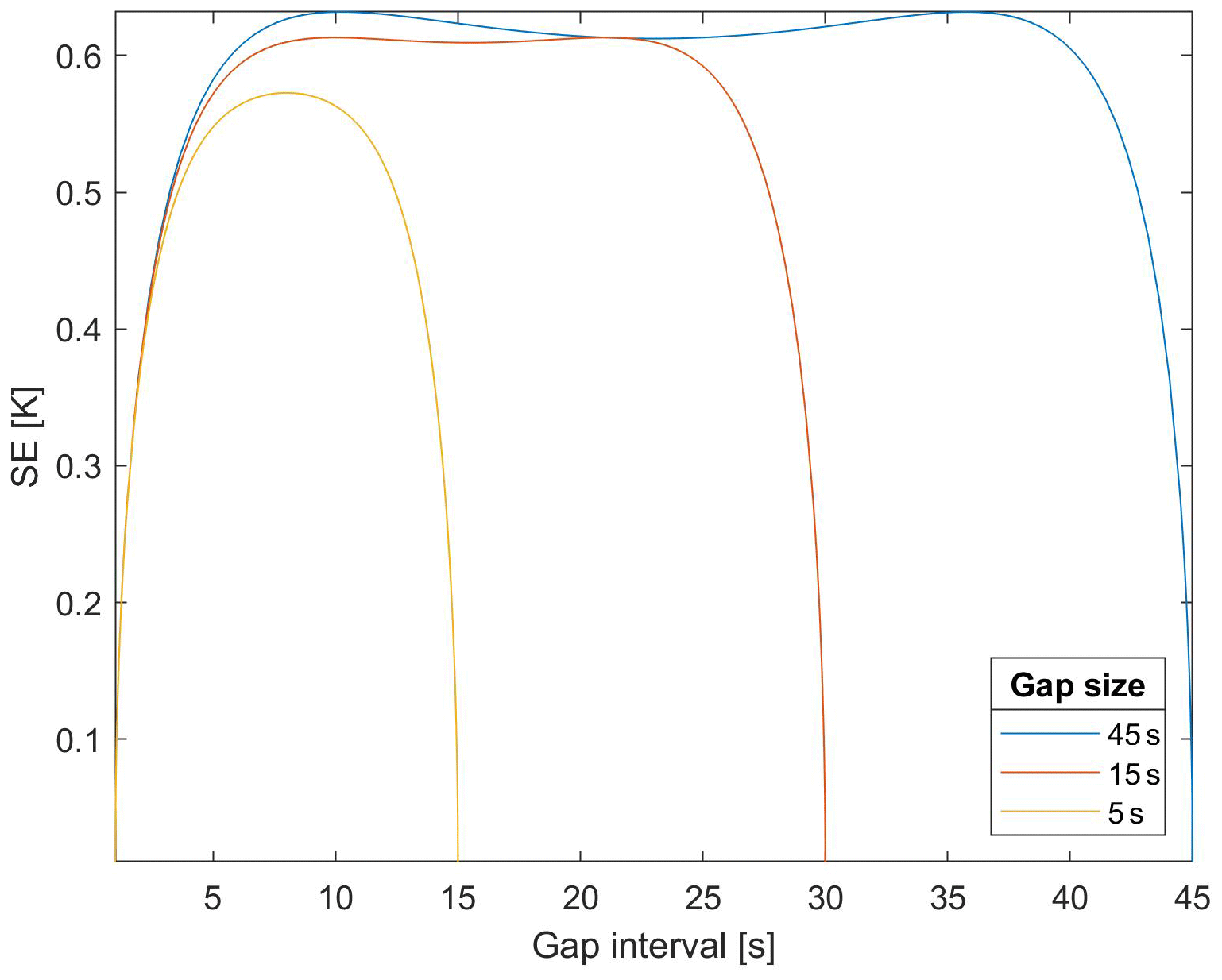
Figure 3Linear interpolation SE, Eq. (8), as a function of the gap time for a GP with σs=0.5 K, σϵ=0.01 K, and θ=3 s. Three gap sizes are considered: 45, 30, and 15 s.
3.2 Gaussian process interpolation
The assumption that the temperature profile y(t) is a realisation of a GP may be extended to cover for a non-constant mean so that, using some basis functions h(), Eq. (1) is rewritten as
with parameter set . In this context, Eq. (3) defines the variance of y(t) conditional on h(t)′β, namely . Let us denote the set of all non-missing observations during the radiosonde flight by Y, denote the matrix of the corresponding basis functions by H, and assume that Ψ is known. Then, the GP interpolation of a missing observation at time t∗ is given by the well-known conditional expectation formula
where ΣY,Y is the covariance matrix of the good observations Y|Hβ and is the covariance vector between the missing observation and Y|Hβ. In addition to point estimation, the GP approach also provides the interpolation standard error:
This formula can be used as an estimate of the interpolation uncertainty, provided that the GP, with the autocovariance given by Eq. (2), is a good description of the problem under study and the true Ψ is approximately known.
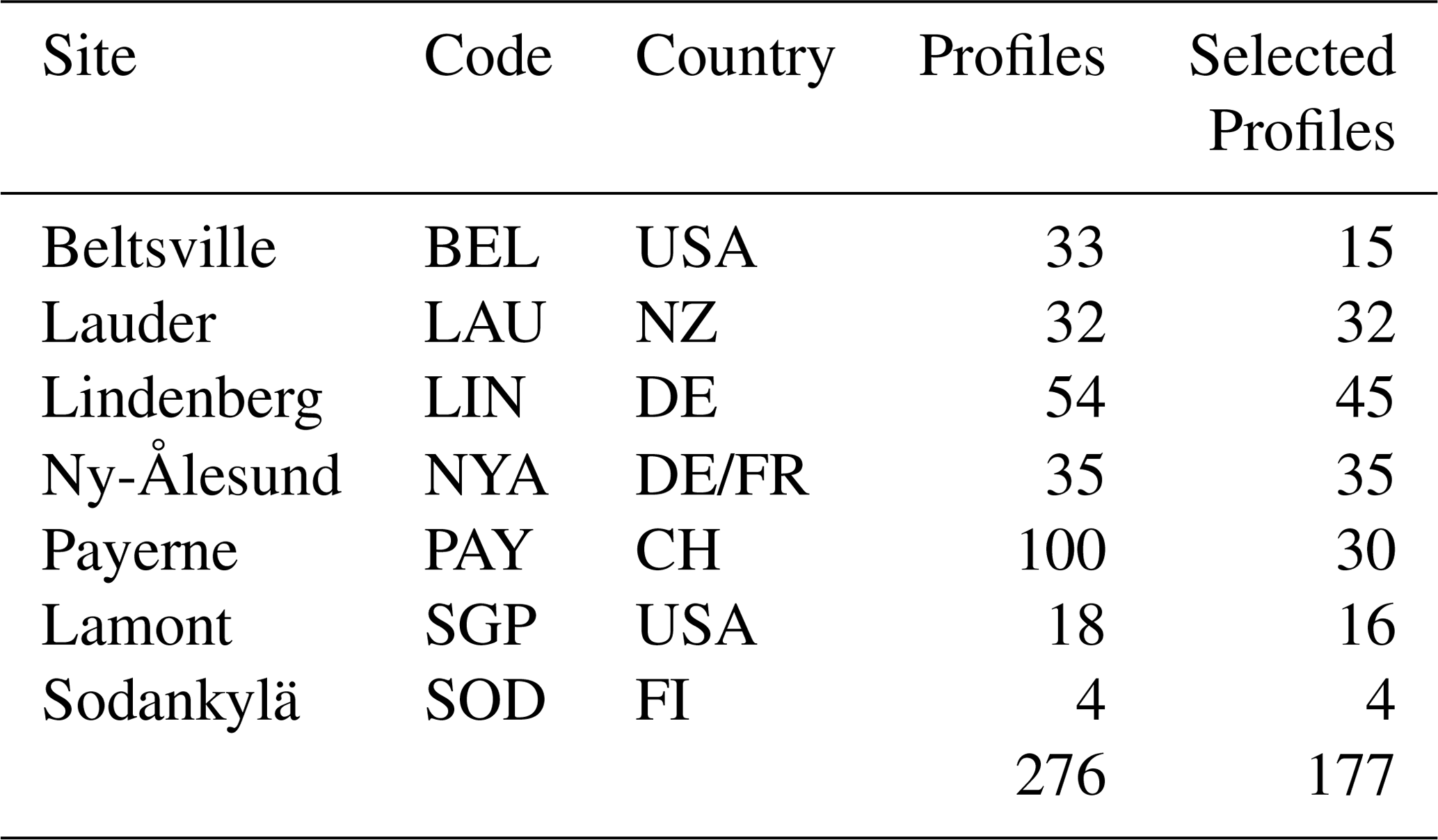
Two data sets provided by the GRUAN Lead Centre (https://www.gruan.org/network/lead-centre, last access: 30 November 2020) and related to the seven GRUAN sites of Table 1 are considered here. One data set is named Few_nan in this paper and contains 276 temperature profiles characterised by “little” missing data. The second data set, named Many_nan, contains 273 profiles with many missing data.
Table 1GRUAN sites included in the Few_nan data set with the respective number of profiles and the number of profiles selected for the analysis, which have gaps shorter than 5 s and a total of fewer then 10 missing values.
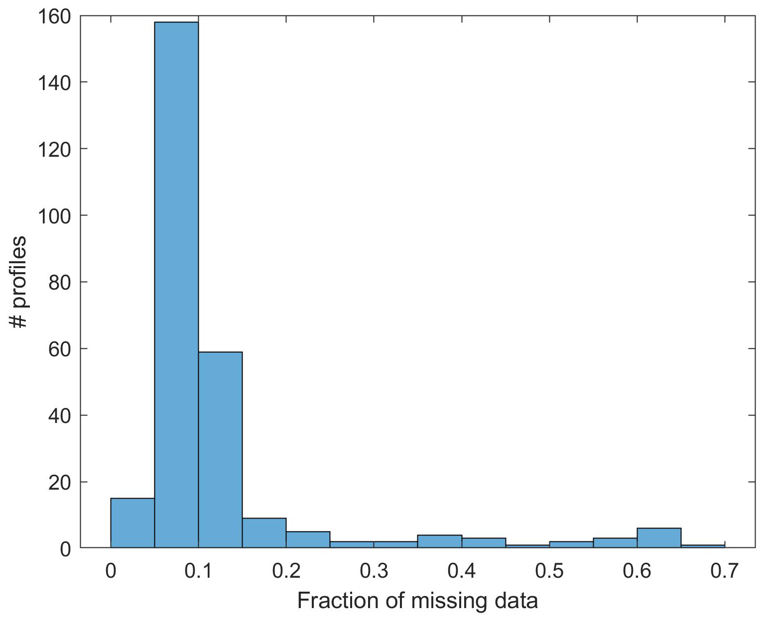
As a preliminary analysis of the bad data set Many_nan, Fig. 5 shows the distribution of the fraction of missing data per launch. The average missing fraction is 0.13, and the average gap length is 3.6 s. These values will be used to set the parameters of the simulated gap patterns in Sect. 5.
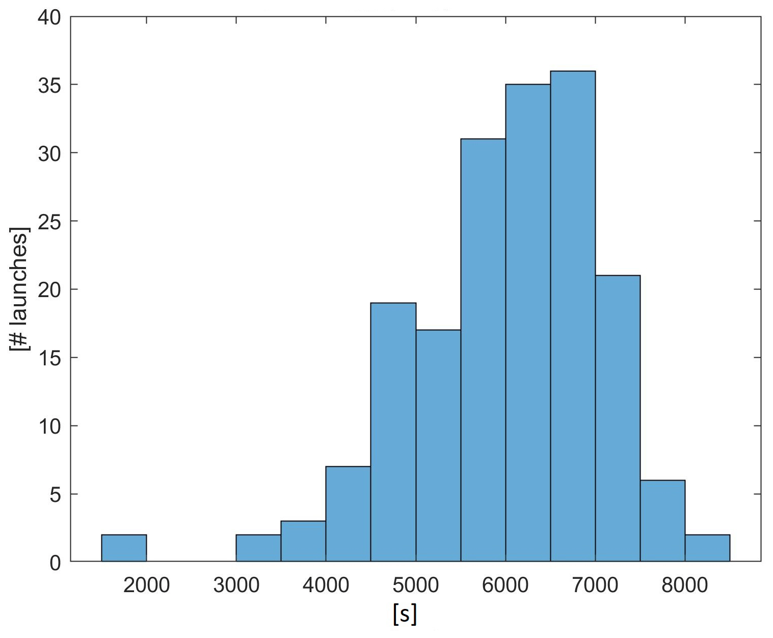
For further interpolation analysis, those profiles in Few_nan with very few missing data are selected. In particular, the L=177 launches which have gaps shorter than 5 s and a total of fewer then 10 missing values per profile have been used in this paper. The profile duration distribution is depicted in Fig. 6, with an average profile duration of about 6000 s. This distribution gives a total of more than 1 million measurements, which will be amplified using the bootstrap technique of Sect. 5.
The block bootstrap is a well-known technique (Politis and Romano, 1994; Mudelsee, 2014) for generating synthetic time series replicates and in this paper is used to construct the cross-validation scheme. Let us consider a fully observed temperature profile – without missing values – and, hence, measurements y taken every second from take-off, : .
This section presents a rule for partitioning each original profile Y as follows:
where YL is the learning set – used for fitting – and Y∗ is the validation set – used for testing the interpolation accuracy and bootstrap correction. In order to construct the testing set, nG gap sequences of average duration μG (s) are extracted from the temperature profile Y and moved to the testing set Y∗. Observe that, if the testing size (average) fraction is denoted by f, then .
The gap scheme is obtained by randomly generating and sorting the nG gap starting points and by building, for each of them, a gap sequence
where the gap duration gj is a geometric random variable with mean μG. In particular, the length gj is truncated at to avoid overlapping among different gap sequences. Let the resulting testing set index be denoted by t∗. Ignoring the above truncation, t∗ has the random dimension and the expected dimension . Hence, the partitioning rule in Eq. (11) is defined by the testing set and the learning set .
We are interested in collecting information about the interpolation error in a dense vertical grid, even if the testing fraction f is small. To accomplish this aim, in the application developed below, the above random extraction process is repeated B times, so that for each observed profile Y, B replications are generated, namely
These replications provide a statistical basis to assess the interpolation uncertainty at all altitudes, especially for those sites with a limited number of available profiles.
The main results of the next section are obtained using linear interpolation of temperature versus time, based on the neighbouring values, and GP interpolation given by the expectation of Y∗ conditional on YL. As in the previous section, let us denote temperature, in Kelvin, by y and flying time, in seconds, by . The total flying time T depends on the single profile and site, but suffixes are not used here for notational simplicity. For each site and launch , we have the interpolated values
where j=1 denotes the linear interpolation of Eq. (5), and j=2 denotes the GP interpolation of Eq. (9).
Each bootstrap replicate , is used first to estimate the GP model coefficients Ψ by the maximum likelihood method, as explained in the next section and denoted by . Then, the interpolated values are computed for the simulated missing times t∗ in the test data set, , and the cross-validation interpolation errors are computed as follows:
Note that each single measurement y and error e are taken at a certain altitude, say , which is known with good precision. As a result, the interpolation MSE and the corresponding root MSE (RMSE) are classified by site, altitude, and gap length:
where ALT identifies a layer of the atmosphere with a thickness between 2 and 7 km, depending on height. The quantity is the average of all testing set terms in the layer ALT, launched from site s and generated using gap size μG. We call ALT the output layering to differentiate from the model-related layering of the next section.
The GP interpolator depends on the local structure , where Ψa(t) is as in Eq. (4). In order to make the local GP modelling feasible and computationally efficient, a block-partitioning structure has been assumed. This assumption amounts to dividing the atmosphere into layers which may differ from the output layers of the previous section. Each atmospheric layer identifies a block, and the variance–covariance matrix for the entire profile is assumed block-diagonal with a constant parameter set Ψa in each layer block. This technique is a special case of the spatial partitioning approach (Heaton et al., 2019), but continuity at the layer borders is ignored here because borders have been deliberately located far from the gaps.
The GP model selection considered the two autocovariance functions γ in Eq. (2), various basis functions h(), and various layerings of the atmosphere to define the appropriate concept of the local model Ψa(t) of Eq. (4). For each layer a, local estimation has been performed using the maximum likelihood method. The above alternatives have been optimised using the RMSE applied to the block-bootstrap replicates of Sect. 5.
Considering the choice of layering resolution, the results were little sensitive to layer-size variations, and a 400 s layer size is used since it provides both a reasonable computing time and a satisfactory atmospheric adaptation. The exponential autocovariance function with p=1 resulted in a smaller cross-validation RMSE compared to the squared exponential one (p=2).
The best results for the basis functions were obtained with a piecewise linear function of time. In this regard, other predictor set-ups were also considered: a piecewise quadratic function of time and vector predictor set-ups, including altitude, coordinates, and wind. Using these more complex models did not result in any relevant improvement to RMSE; still worse, it resulted in problems concerning the singularity of the information matrix at various combinations of sites and layers. Hence, invoking Occam's razor and looking for a robust and general model set-up, we settled on using the simplest piecewise linear function of time.
This section's bootstrap campaign aims to assess the uncertainty of the linear interpolation, Eqs. (5) and (8), and of the GP interpolation, Eqs. (9) and (10). The cross-validation design is based on a 4×3 combination of gap sizes μG and missing fractions f, centred on the characteristics of the Many_nan data set. In detail, we use μG=4, 10, 30, and 60 s and f=0.05, 0.13, and 0.20. Moreover, for uncertainty estimates with a high vertical density, the block-bootstrap validation of Sect. 5 is replicated B=50 times, giving a data set with more than 51 million measurements for each combination of μG and f.
Table 2Comparison of cross-validation RMSEs between GP and linear interpolation for increasing average gap length μG=4, 10, 30 and 60 s. Cross-validation is based on B=50 block-bootstrap replications, each with missing fraction f=0.13. The last line reports the total number of profiles and the average RMSE.
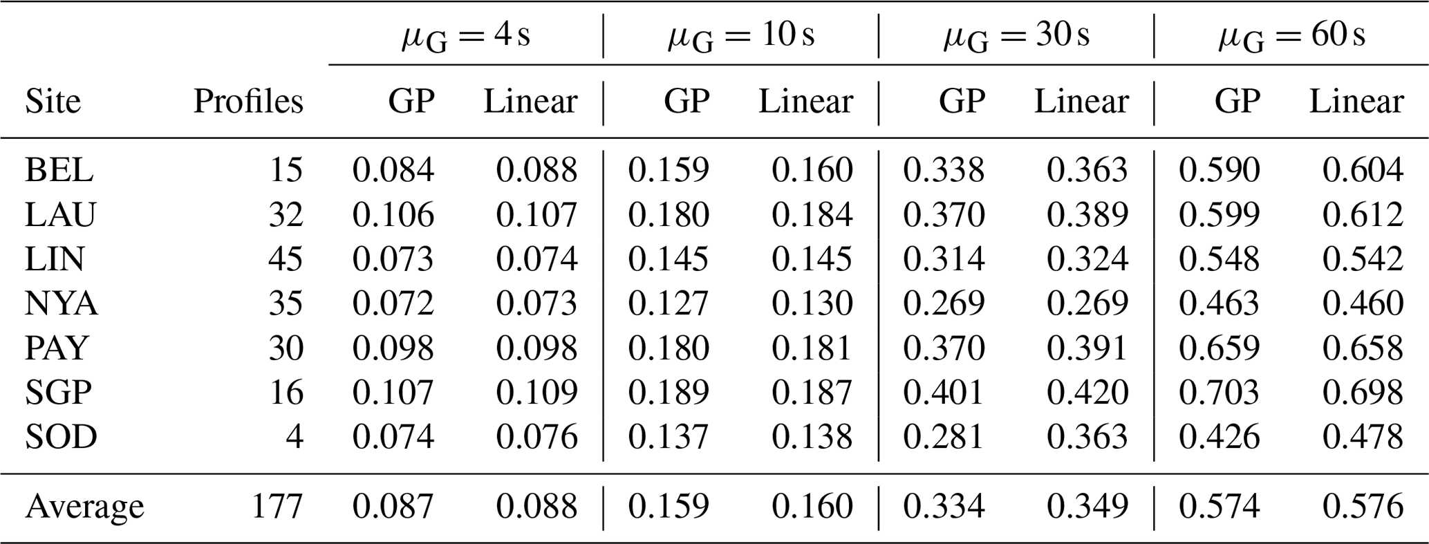
Table 2 summarises the RMSEs of both the linear and GP interpolations. Overall, the average interpolation uncertainty is smaller than 0.1 K for little gaps (μG=4 s), increases to about 0.16 K for medium gaps (μG=10 s), and increases further to 0.35 and 0.58 K for large and very large gaps (μG=30 and 60 s), respectively.
When comparing the two interpolation approaches, Table 2 shows that they have very close RMSEs. Indeed, not only do the linear and GP interpolations have close performances, but also, for any practical purposes, they are exchangeable since the mean absolute difference between the two is smaller than 0.01 K. Hence, in the rest of this paper, we will not replicate figures and results for both interpolation methods.
Figure 7 depicts the linear interpolation uncertainty at each GRUAN site using the RMSE based on Eq. (12). Here and in the rest of this section, for simplicity, the largest average gap size μG=60 s is omitted. The clustered pattern of the nine curves clearly shows that the missing fraction f has a minor influence on uncertainty in the range 0.05–0.20, which is the range of interest for meaningful practical applications. Hence, for the rest of the paper, we will consider only the missing fraction f=0.13. Moreover, considering jointly Fig. 7 and Table 2, Lamont, Payerne, and Lauder have slightly larger RMSEs at all gap sizes.
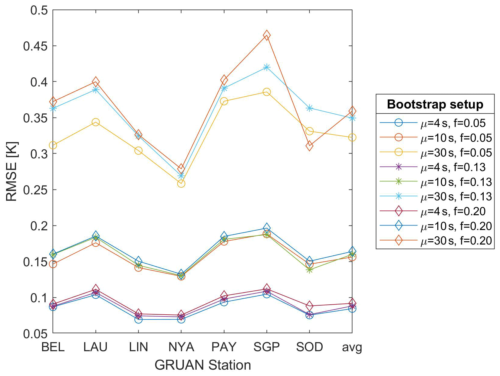
Figure 7Linear interpolation uncertainty by GRUAN site and average gap size μG=4, 10, and 30 s. The cross-validation uncertainty (y axis) is based on the root mean square error (RMSE) for missing fractions f=0.05, 0.13, and 0.20.
Figure 8 depicts the vertical behaviour of the linear interpolation uncertainty at GRUAN sites, with average gap size increasing from the top to bottom panel. As expected, the uncertainty's minimum is near the tropopause. Moreover, after a fast increase, it stabilises at a value which is often larger than the lower atmosphere uncertainty level. The various sites have globally similar values, but again, Lamont, Payern, and Lauder typically have the largest values.
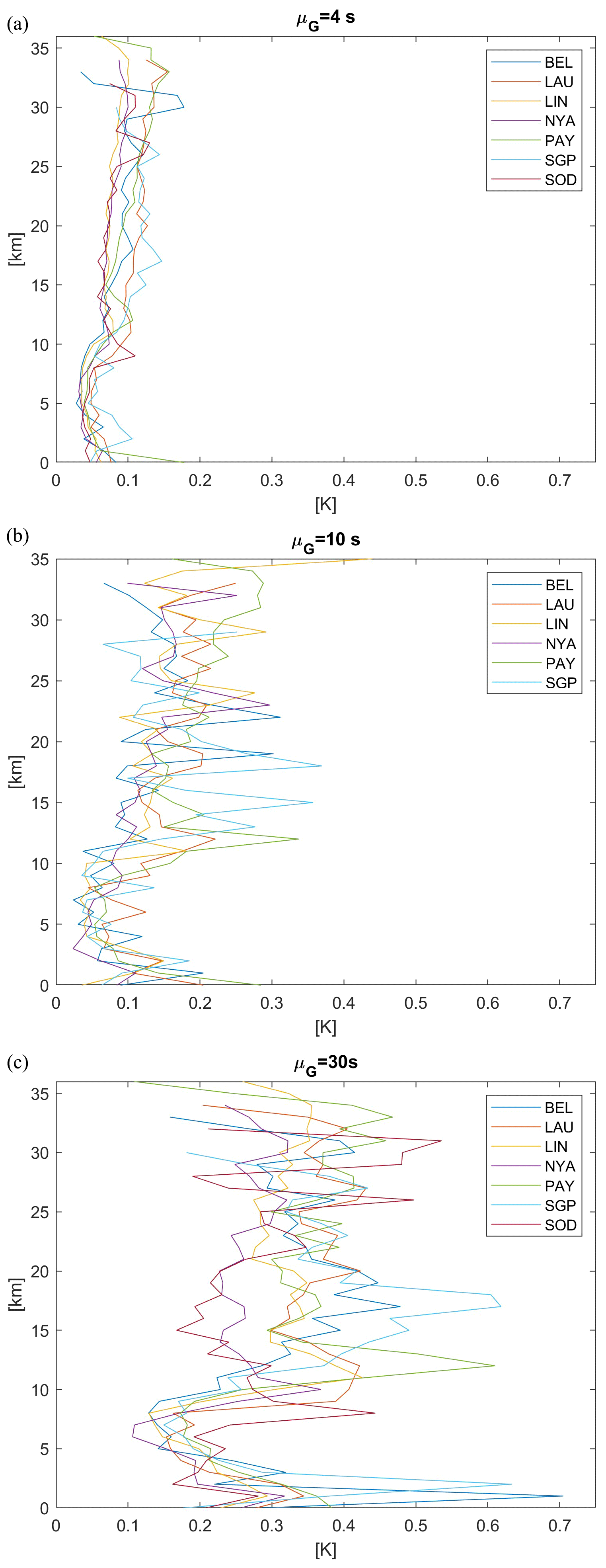
Figure 8Linear interpolation uncertainty of GRUAN sites. The cross-validation uncertainty (x axis) is based on the RMSE and missing fraction f=0.13. (a) Average gap size is μG=4 s; (b) average gap size is μG=10 s; (c) average gap size is μG=30 s.
In order to re-interpret the GP-based linear interpolation uncertainty formula of Figs. 3 and 4, we consider the ensemble of all the estimated local GP model parameters set Ψ from the entire cross-validation exercise. Coherently with the known small intrinsic error declared by Vaisala, Fig. 9a shows very small values of σϵ. Moreover, from Fig. 9b, we see that the values σs<1 K are common and, in particular, σs=0.5 K used in Figs. 3 and 4 is quite plausible. Eventually, Fig. 9c shows that the correlation range θ may be easily between 1 and 15 min.
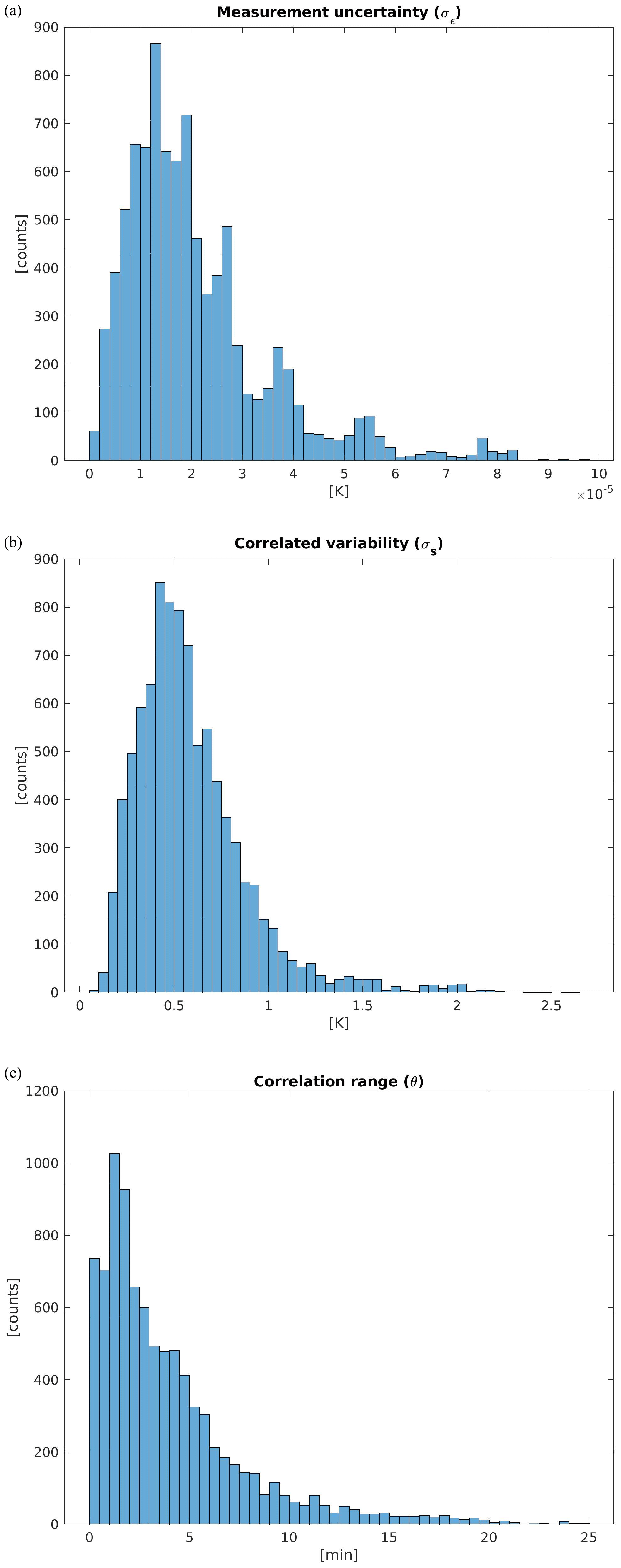
Figure 9Frequency distribution of estimated GP model parameters from all bootstrapped profiles and all model-related atmospheric layers. (a) σϵ [K]; (b) σs [K]; (c) correlation range θ (min). The average gap size is μG=10 s and the missing fraction is f=0.13.
8.1 Interpolation distance
In general, the connection between the uncertainty curves of Figs. 3 and 4 and the cross-validation evidence are worth studying. Considering both the gap size and the distance from the observations at various altitudes gives rise to hard-to-manage curve plots and a multiplicity of results. For this reason, the subsequent analysis is based on the interpolation distance in seconds, which is denoted by d and given by the geometric mean of the temporal distances of all missing data from the closest observations y− and y+ in the notation of Sect. 3.
Figure 10 depicts the cross-validation RMSEs of the linear interpolation as a function of interpolation distance by altitude, namely
where is the average of all the cross-validation terms with altitude in the layer ALT and interpolation distance d. We note that, in order to have high sampling information for both low and high interpolation distances, the graph is obtained by merging the results obtained for μG=10 and 30 s. We also note that, thanks to the geometric distribution used in the block-bootstrap procedure in Sect. 5, we are able to consider distances larger than 30 s. In particular, Fig. 10 only depicts interpolation distances up to 70 s. Indeed, the block bootstrap with an average distance of μG=30 s provides little testing data at larger distances, especially at high altitudes. Of course, using the same approach, longer interpolation distances may be easily explored by generating testing sets with larger μG.
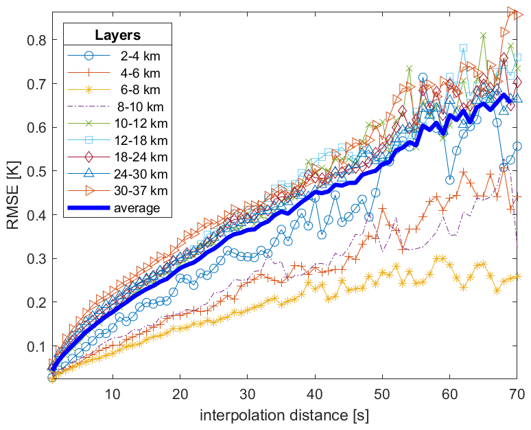
Figure 10Each line shows the cross-validation RMSE of linear interpolation as a function of the interpolation distance (s) for a specific atmospheric layer in the range of 2–37 km. The interpolation distance (x axis) is given by the geometric mean of the distances of all missing data from the closest good data, y− and y+. The graph is obtained my merging the block-bootstrap simulations with average gap sizes μG=10 and 30 s.
In addition, Fig. 11 depicts the corresponding graph for the linear interpolation , given by Eq. (8), and quadratically averaged over site s, launch l, and bootstrap replication b, namely
The corresponding graph for the GP–SE of Eq. (10) is not reported here because it gives very close results. Indeed, not only are the two interpolation methods exchangeable, as noticed above, but their SEs are also very close, with a mean absolute difference between the two of less than 0.005 K.
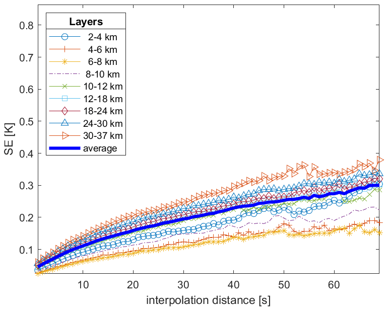
Figure 11Each line shows the linear interpolation SE as a function of the interpolation distance (s) for a specific atmospheric layer in the range of 2–37 km. The depicted SE is the quadratic average of Eq. (8) for each altitude and interpolation distance in the validation data set. The interpolation distance (x axis) is given by the geometric mean of the distances of all missing data from the closest good data, y− and y+. The graph is obtained my merging the block-bootstrap simulations with average gap sizes μG=10 and 30 s.
Figures 10 and 11 have similar increasing behaviour, but the average linear interpolation SE is generally smaller than the corresponding RMSE and approximately equal at the very short distance d=1 s. From Eq. (7), we expect that they differ by a quantity depending on the measurement error uncertainty, σϵ. Recalling Fig. 9, the latter is very small, and it is not enough to explain such a discrepancy. Indeed, Eq. (7) would hold exactly if (i) the used GP were a perfect model for our data, (ii) its coefficients Ψ were known exactly, and (iii) the cross-validation estimation of the RMSE were exact. The latter two conditions hold approximately due to the large data set used. Hence, the SE underestimates the “true” interpolation uncertainty, primarily due to the GP model approximation.
For the above reasons, we propose a bootstrap-corrected interpolation uncertainty estimate by merging the information of the single profile (s,l) captured by the corresponding GP and the average offset of the uncertainty given by the RMSE:
In practice, the first summand, SE, must be computed for every single profile, while the term based on MSE may be implemented as a lookup table.
8.2 Practical aspects
As an illustration of the method, the profile of the Sodankylä site on 3 March 2017 12:00 UTC is considered in Fig. 12a. This profile has T=4722 measurements and no original missing values. Using the block bootstrap, 563 measurements have been deleted (pseudo-missing), generating gap lengths between 1 and 24 s. From a practical point of view, such missing rates and gap lengths can be considered a relatively common, yet serious, case for interpolation. In Fig. 12b, the results of the previous subsection, based on the entire data set, are used to show both ± the GP uncertainty of Eq. (8) and ± the bootstrap uncertainty of Eq. (15), computed at the interpolated pseudo-missing values. The result is that the bootstrap-corrected interpolation uncertainty never exceeds 0.3 K along this profile. In doing this computation, Eqs. (13) and (14) are implemented as lookup tables with entries geometric distance and altitude.

Figure 12RS42 temperature profile at the Sodankylä site on 3 March 2017 12:00 UTC. (a) Observation is in blue and block-bootstrap pseudo-missing are in red. (b) ± Linear interpolation uncertainty of pseudo-missing values; GP uncertainty (Eq. 8) is in dark blue; bootstrap uncertainty (Eq. 15) is in orange.
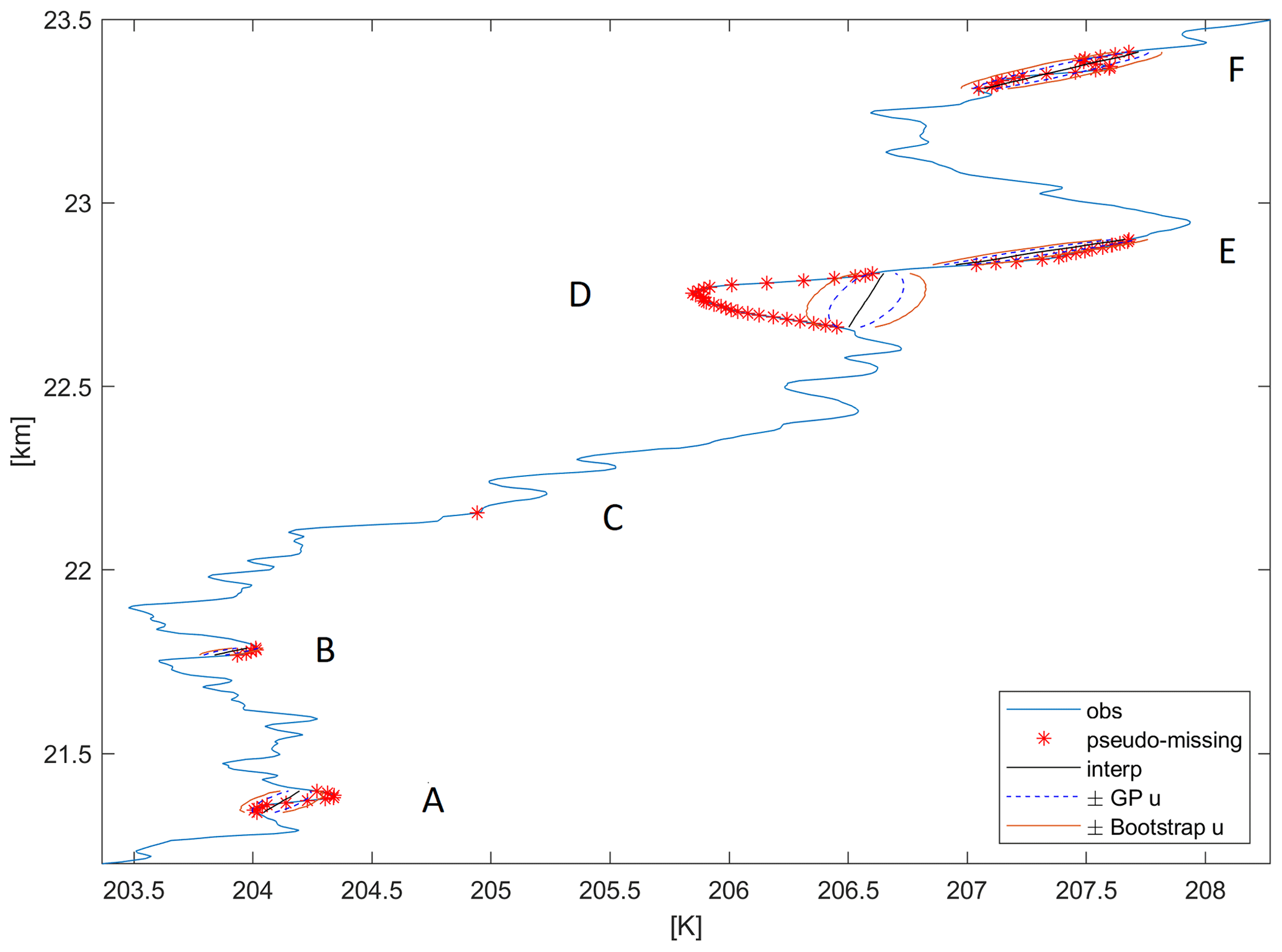
Figure 13Detail of the RS42 temperature profile at the Sodankylä site on 3 March 2017 12:00 UTC, around 22.5 km altitude. Observations are in blue, block-bootstrap pseudo-missing are in red, and the corresponding five gaps are labelled A–F; linear interpolation is in black; ± GP uncertainty, Eq. (8), is in dashed blue; ± Bootstrap-corrected uncertainty, Eq. (15), is in orange.
Figure 13 zooms in on the above profile at around 22.5 km height and shows in detail the interpolation of a single point gap (C), two small gaps (A, B), and three larger gaps (D–F). For Gap C, the uncertainty is almost negligible using both methods. As far as the gap size increases, both the uncertainty and the difference between the two methods increase. In the most extreme case, Gap D, the bootstrap uncertainty is about twice the uncorrected amount. Of course, this is the case where any interpolation method but Delphi's oracle would fail. Nonetheless, the error (interpolated minus observed) is approximately 3u in absolute value, where u is the bootstrap-corrected uncertainty of Eq. (15). Hence, also in this difficult interpolation case, our bootstrap-corrected approach provides a sensible estimate of the uncertainty.
It follows that the implementation of GRUAN data processing providing interpolated temperature profiles along with their uncertainty requires some effort divided into two different phases. First, massive GP offline computation is needed to prepare the lookup table related to Eqs. (13) and (14). Second, for each profile, an online local GP calibration is needed to provide the SE (Eq. 8) for the interpolated values. After this processing, Eq. (15) easily gives the corrected interpolation uncertainty.
This paper offers a multifaceted assessment of the interpolation uncertainty of Vaisala RS41 temperature profiles at various altitudes, using an extensive data set from seven GRUAN sites. Moreover, it provides a general framework for the interpolation of generic atmospheric profiles.
Two complementary uncertainty approaches have been developed and integrated. The first is a cross-validation approach based on block bootstrap, which shows that the average of the root mean square error of linear interpolation is about 0.1 K for small gaps, which increases up to 0.58 K for gaps of an average duration of 60 s. These results may be made operational as lookup tables characterising interpolation uncertainty with entry altitude and interpolation distance. The resulting lookup table could be made available to the scientific community.
Since the cross-validation outputs are averages, the individual profile contribution to the uncertainty is not considered. Hence, the second approach addresses interpolation uncertainty using Gaussian process assumptions. This approach allows for obtaining a formula for the interpolation uncertainty which depends on the autocorrelation structure of each single profile.
Integrating the above two approaches, a bootstrap-corrected formula for the individual interpolation uncertainty is proposed. Based on these results, a future version of GRUAN data processing could implement interpolated temperature profiles, uncertainty included.
The extension of this approach to other essential climate variables (ECVs) and/or other instruments requires some consideration. From the modelling point of view, provided that enough field data are available, the extension is relatively straightforward. Indeed, the approach is quite general, and model selection and optimisation are data-driven. Hence, similar results may be expected for temperature profiles obtained by other instruments, provided that vertical resolution and instrumental error are comparable to the present case. Further, similar results are also expected for other smooth variables, such as pressure.
On the other hand, the interpolation uncertainty could be greater for ECVs which are known to have large variations in the small scale. For example, relative humidity commonly shows highly intermittent profiles in the troposphere, with very large and very fast-changing gradients. In these cases, we can expect that the cross-validation uncertainty could be high even for small gaps. In addition, the vertical autocorrelation could have a shorter range, and the corresponding GP model could provide interpolation uncertainties close to the white noise case considered in Sect. 3.
To see Eq. (8), let us rewrite the interpolation error of Eq. (6) as follows:
where as in Sect. 3.1, is a vector of constants for fixed times and is a stochastic vector. With these symbols, Eq. (8) may be written as
where Σu is the variance–covariance matrix of u given by
The conclusion follows by straightforward algebra.
The underlying MATLAB code is available from the corresponding author upon request. The data are available from the GRUAN Lead Centre (https://www.gruan.org/, last access: 30 November 2020) upon request.
Sections 1 and 9 are written together. Section 2 is due to MS and CvR. Sections 2–8 are due to AF.
The authors declare that they have no conflict of interest.
The authors wish to thank the GRUAN Quality Task Force for the extensive discussions.
This paper was edited by Brian Kahn and reviewed by two anonymous referees.
Alegria, A., Caro, S., Bevilacqua, M., Porcu, E., and Clarke, J.: Estimating covariance functions of multivariate skew-Gaussian random fields on the sphere, Spat. Stat.-Neth., 22, 388–402, 2017. a
Bodeker, G. E., Bojinski, S., Cimini, D., Dirksen, R. J., Haeffelin, M., Hannigan, J. W., Hurst, D. F., Leblanc, T., Madonna, F., Maturilli, M., Mikalsen, A. C., Philipona, R., Reale, T., Seidel, D. J., Tan, D. G. H., Thorne, P. W., Vömel, H., and Wang, J.: Reference Upper-Air Observations for Climate: From Concept to Reality, B. Am. Meteorol. Soc., 97, 123–135, https://doi.org/10.1175/BAMS-D-14-00072.1, 2016. a
Ceccherini, S., Carli, B., Tirelli, C., Zoppetti, N., Del Bianco, S., Cortesi, U., Kujanpää, J., and Dragani, R.: Importance of interpolation and coincidence errors in data fusion, Atmos. Meas. Tech., 11, 1009–1017, https://doi.org/10.5194/amt-11-1009-2018, 2018. a
Cressie, N. and Wikle, C.: Statistics for Spatio-Temporal Data, Wiley, New York, USA, 2011. a, b
Dirksen, R. J., Sommer, M., Immler, F. J., Hurst, D. F., Kivi, R., and Vömel, H.: Reference quality upper-air measurements: GRUAN data processing for the Vaisala RS92 radiosonde, Atmos. Meas. Tech., 7, 4463–4490, https://doi.org/10.5194/amt-7-4463-2014, 2014. a
Dirksen, R. J., Bodeker, G. E., Thorne, P. W., Merlone, A., Reale, T., Wang, J., Hurst, D. F., Demoz, B. B., Gardiner, T. D., Ingleby, B., Sommer, M., von Rohden, C., and Leblanc, T.: Managing the transition from Vaisala RS92 to RS41 radiosondes within the Global Climate Observing System Reference Upper-Air Network (GRUAN): a progress report, Geosci. Instrum. Method. Data Syst., 9, 337–355, https://doi.org/10.5194/gi-9-337-2020, 2020. a
Fassò, A., Ignaccolo, R., Madonna, F., Demoz, B. B., and Franco-Villoria, M.: Statistical modelling of collocation uncertainty in atmospheric thermodynamic profiles, Atmos. Meas. Tech., 7, 1803–1816, https://doi.org/10.5194/amt-7-1803-2014, 2014. a
Finazzi, F., Fassò, A., Madonna, F., Negri, I., Sun, B., and Rosoldi, M.: Statistical harmonization and uncertainty assessment in the comparison of satellite and radiosonde climate variables, Environmetrics, 30, 1–17, https://doi.org/10.1002/env.2528, 2019. a
Genton, M.: Classes of Kernels for Machine Learning: A Statistics Perspective, J. Mach. Learn. Res., 2, 299–312, 2001. a
Heaton, M. J., Datta, A., Finley, A. O., Furrer, R., Guinness, J., Guhaniyogi, R., Gerber, F., Gramacy, R. B., Hammerling, D., Katzfuss, M., Lindgren, F., Nychka, D. W., Sun, S., and Zammit-Mangion, A.: A Case Study Competition Among Methods for Analyzing Large Spatial Data, J. Agr. Biol. Envir. St., 24, 398–425, https://doi.org/10.1007/s13253-018-00348-w, 2019. a
Ignaccolo, R., Franco-Villoria, M., and Fassò, A.: Modelling collocation uncertainty of 3D atmospheric profiles, Stoch. Env. Res. Risk A., 29, 417–429, 2015. a
Immler, F. J., Dykema, J., Gardiner, T., Whiteman, D. N., Thorne, P. W., and Vömel, H.: Reference Quality Upper-Air Measurements: guidance for developing GRUAN data products, Atmos. Meas. Tech., 3, 1217–1231, https://doi.org/10.5194/amt-3-1217-2010, 2010. a
Kimeldorf, G. S. and Wahba, G.: A correspondence between Bayesian estimation on stochastic processes and smoothing by splines, Ann. Math. Stat., 41, 495–502, 1970. a
Mudelsee, M.: Climate Time Series Analysis – Classical Statistical and Bootstrap Methods, 2nd edn., Springer, Berlin, Germany, 2014. a, b
Politis, D. and Romano, J.: The stationary bootstrap, J. Am. Stat. Assoc., 89, 1303–1313, 1994. a, b
Porcu, E., Bevilacqua, M., and Genton, M.: Spatio-Temporal Covariance and Cross-Covariance Functions of the Great Circle Distance on a Sphere, J. Am. Stat. Assoc., 111, 888–898, 2016. a
Rasmussen, C. E. and Williams, C. K. I.: Gaussian Processes for Machine Learning, MIT Press, Boston, USA, 2006. a, b
Seidel, D. J., Berger, F. H., Immler, F., Sommer, M., Vömel, H., Diamond, H. J., Dykema, J., Goodrich, D., Murray,W., Peterson, T., Sisterson, D., Thorne, P., and Wang, J.: Reference Upper-Air Observations for Climate: Rationale, Progress, and Plans, B. Am. Meteorol. Soc., 90, 361–369, 2009. a
Sinyuk, A., Holben, B. N., Eck, T. F., Giles, D. M., Slutsker, I., Korkin, S., Schafer, J. S., Smirnov, A., Sorokin, M., and Lyapustin, A.: The AERONET Version 3 aerosol retrieval algorithm, associated uncertainties and comparisons to Version 2, Atmos. Meas. Tech., 13, 3375–3411, https://doi.org/10.5194/amt-13-3375-2020, 2020. a
Sofieva, V. F., Dalaudier, F., Kivi, R., and Kyrö, E.: On the variability of temperature profiles in the stratosphere: Implications for validation, Geophys. Res. Lett., 35, L23808, https://doi.org/10.1029/2008GL035539, 2008. a
Sun, B., Reale, A., Seidel, D. J., and Hunt, D. C.: Comparing radiosonde and COSMIC atmospheric profile data to quantify differences among radiosonde types and the effects of imperfect collocation on comparison statistics, J. Geophys. Res., 115, D23104, https://doi.org/10.1029/2010JD014457, 2010. a
Verhoelst, T., Granville, J., Hendrick, F., Köhler, U., Lerot, C., Pommereau, J.-P., Redondas, A., Van Roozendael, M., and Lambert, J.-C.: Metrology of ground-based satellite validation: co-location mismatch and smoothing issues of total ozone comparisons, Atmos. Meas. Tech., 8, 5039–5062, https://doi.org/10.5194/amt-8-5039-2015, 2015. a
- Abstract
- Introduction
- Data processing and interpolation
- Interpolation uncertainty
- Data
- Block-bootstrap cross-validation scheme
- Cross-validation
- Modelling details
- Results
- Conclusions
- Appendix A: Linear interpolation uncertainty
- Code and data availability
- Author contributions
- Competing interests
- Acknowledgements
- Review statement
- References