Detecting turbulent structures on single Doppler lidar large datasets: an automated classification method for horizontal scans

Medium-to-large fluctuations and coherent structures (mlf-cs's) can be observed using horizontal scans from single Doppler lidar or radar systems. Despite the ability to detect the structures visually on the images, this method would be time-consuming on large datasets, thus limiting the possibilities to perform studies of the structures properties over more than a few days. In order to overcome this problem, an automated classification method was developed, based on the observations recorded by a scanning Doppler lidar (Leosphere WLS100) installed atop a 75 m tower in Paris's city centre (France) during a 2-month campaign (September–October 2014). The mlf-cs's of the radial wind speed are estimated using the velocity–azimuth display method over 4577 quasi-horizontal scans. Three structure types were identified by visual examination of the wind fields: unaligned thermals, rolls and streaks. A learning ensemble of 150 mlf-cs patterns was classified manually relying on in situ and satellite data. The differences between the three types of structures were highlighted by enhancing the contrast of the images and computing four texture parameters (correlation, contrast, homogeneity and energy) that were provided to the supervised machine-learning algorithm, namely the quadratic discriminant analysis. The algorithm was able to classify successfully about 91 % of the cases based solely on the texture analysis parameters. The algorithm performed best for the streak structures with a classification error equivalent to 3.3 %. The trained algorithm applied to the whole scan ensemble detected structures on 54 % of the scans, among which 34 % were coherent structures (rolls and streaks).

1 Introduction

Turbulent flows are motions characterized by high unpredictability. Nevertheless, coherent structures are developed in these flows (Tur and Levich, 1992). The principal aspect that determines a coherent structure is the maintenance of the phase-averaged vorticity of the turbulent fluid mass over the spatial extent of the flow structure (Hussain, 1983). The most typical types of coherent structures are presented in the review of Young et al. (2002), who classified structures into three characteristic types: turbulent streaks, convective rolls and gravity waves. Several studies have been carried out to examine the effect of the coherent turbulent structures in the dispersion of pollutants by utilizing boundary layer simulations. The results of these studies indicate that the coherent structures can play a significant role in the pollutants' concentrations (Aouizerats et al., 2011; Soldati, 2005). Furthermore, Sandeepan et al. (2013) have demonstrated via simulations that the pollutants' concentrations can alternate from low to high during coherent-structure events. It is therefore important to be able to identify structures in the atmosphere and observe them in an efficient and consistent way. The term coherent structures in the aforementioned studies refers exclusively in the atmospheric flow, and it is the main focus in this study. This term is also encountered in studies at the laboratory scale described as hairpins or packets (Adrian, 2007; Hutchins and Marusic, 2007), but these are out of the scope of this study.

Turbulent streaks are structures aligned with the horizontal wind with alternating stripes of stronger horizontal wind associated with a subsidence and stripes of weaker horizontal wind associated with an ascendance (Khanna and Brasseur, 1998). The high wind shear between the surface layer and the lower planetary boundary layer (PBL) can lead to the formation of the turbulent streaks in the surface layer that may extend to the mixed layer. Neutral or near-neutral stratification favours the formation of streaks, though they may also form during stable and unstable conditions (Khanna and Brasseur, 1998). The physics behind their formation differs as the contribution of buoyancy varies in relation to the atmospheric conditions (Moeng and Sullivan, 1994). Formation, evolution and decay of streaks are rather short, equivalent to several tens of minutes, before they regenerate. The average streak spacing is usually hundreds of metres (Drobinski and Foster, 2003). In the mixed layer, horizontal roll vortices, also known as convective rolls, develop roughly aligned with the mean wind (LeMone, 1972). Favourable conditions for the development and maintenance of convective rolls are the spatial variations of surface-layer heat flux, the low-level wind shear and the relatively homogeneous surface characteristics (Weckwerth and Parsons, 2006). As the rolls rotate in the vertical plane, they generate ascending and descending motions. These motions under convective conditions can form clouds in rows separated by clear-sky areas known as cloud streets, which is a characteristic visual feature used to identify rolls (Lohou et al., 1998). The rolls usually extend from the surface to the capping inversion with a large variety of horizontal sizes from a few kilometres to few tens of kilometres. They are characterized by a long lifespan of hours or even days as opposed to the short lifespan of the streaks (Drobinski and Foster, 2003). Young et al. (2002) distinguish rolls in narrow mixed-layer rolls, where the ascending air masses are one thermal wide (Weckwerth et al., 1999), and wide mixed-layer rolls, where multiple thermals are grouped within each ascending area (Brümmer, 1999). As Young et al. (2002) stated, both types of rolls can be distinguished visually, with the narrow rolls having the form of a “string of pearls”, whereas the wide rolls look like a “band of froth”.

Remote sensors are exceptionally useful for the identification of coherent structures. Their ability to scan large areas in a short period is advantageous compared to in situ measurements (Kunkel et al., 1980). Lhermitte (1962) and Browning and Wexler (1968) were the first to implement the velocity–azimuth display (VAD) technique, also known as the plan position indicator (PPI) method, using Doppler radars. The PPI technique provides conical scans or even horizontal surface scans with the appropriate combination of elevation and azimuth angles. Kropfli and Kohn in 1978 were able to study horizontal roll structures by using a dual-Doppler radar in order to observe the wind field in the three dimensions. Several studies followed for different types of radars with more efficient configurations (Kelly, 1982; Lohou et al., 1998; Reinking et al., 1981). Weckwerth et al. (1999) were able to study the evolution of horizontal convective rolls by combining Doppler radar observations with meteorological measurements, radiosondes, flight measurements and satellite images. In recent years, various studies have been carried out by using lidars only. It has been well established that the PPI method can also be applied to Doppler lidars (Cariou et al., 2007; Vasiljević et al., 2016) with the possibility to compute the mean wind profile by using a modified version of the VAD method as has been demonstrated in the studies of Banta et al. (2002) and Chai et al. (2004). Depending on the selected scanning method of the Doppler lidar, it is possible to observe coherent structures in the atmospheric surface layer (Drobinski et al., 2004) as well as in the mixed layer (Drobinski et al., 1998). Newsom et al. (2008) and Iwai et al. (2008) introduced the dual-Doppler lidar method and revealed its benefits in the observation of coherent structures. This method was further improved by Träumner et al. (2015) using an optimized dual-Doppler technique. They were able to identify different type of structures including elongated areas resembling turbulent streaks. They combined quantitative characteristics of the coherence such as the integral scales and the anisotropy coefficients, obtained by a two-dimensional autocorrelation algorithm, with the visual observation of the scans. However, the subjective classification by observing the images is a time-consuming approach and non-systematic. Furthermore, the use of two Doppler lidars is limited to the institutes that can afford such a high cost and collaborations on short-term campaigns. A much less expensive approach, and suitable for long periods, is to detect the passage of the structures on sonic anemometer time series. For instance, Barthlott et al. (2007) analysed 10 months of data from a meteorological tower located in the surface layer 20 km south of Paris, France, and they observed coherent structures for 36 % of the cases. However, their study is limited to point measurements instead of a larger wind field that it is possible to observe via a lidar.

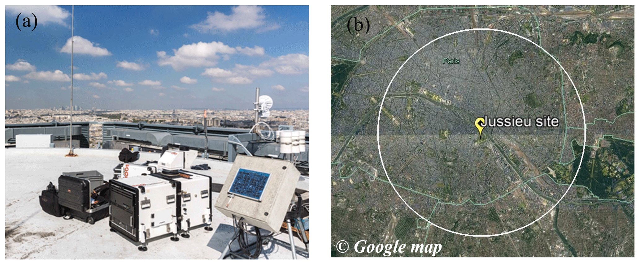
Figure 1 (a) The Doppler lidar installed on the tower roof during the VEGILOT campaign and (b) the measurement site in Paris with inside a circle with a 10 km diameter demonstrating the maximum range of the PPI surface scan (© Google Earth satellite image).

This study aims to identify the medium-to-large fluctuations and coherent structures (mlf-cs's) on single Doppler lidar horizontal scans and develop an automatic classification process based on the combination of texture analysis and a supervised machine-learning technique, namely the quadratic discriminant analysis (QDA), in order to handle large datasets. Texture analysis is an effective way to evaluate the distribution of the values within an image (Castellano et al., 2004). It is widely used in various scientific fields in order to classify images, covering meteorology (Alparone et al., 1990), medical studies (Holli et al., 2010) and forestry (Kayitakire et al., 2006). There is a lack of long-term studies of structures based on lidar observations, and the aforementioned automatic classification process can stimulate the interest in this research field. More particularly, it could facilitate the statistical analysis of the physical parameters of the structures, e.g. the structure size as a function of the height of the planetary boundary layer (PBL). Furthermore, it will enable us to study the transitions between structures and how these are associated with the atmospheric conditions. Finally, the impact of the structures on pollutants' concentrations could be examined for long-term studies under stable and unstable conditions. The classification method relies on the observations of radial wind speed recorded using a scanning Doppler lidar settled atop a 75 m high tower in the centre of Paris, during a 2-month period in late summer and early fall. Section 2 presents the experimental setup of the study. The methodology for the identification and classification of the mlf-cs's is demonstrated in Sect. 3. Subsequently, the results of the classification for the training ensemble as well as for the whole dataset are displayed in Sect. 4. Finally, the key points of the paper are summarized in Sect. 5.

2 Experimental setup

A 2-month measurement campaign (4 September–6 November 2014) was carried out in order to study the exchange processes of ozone and aerosols in the area in the framework of the VEGILOT (VEGétation et ILOT de chaleur urbain; vegetation and urban heat island) project in the urban area of Paris (Klein et al., 2019). The Leosphere WLS100 Doppler lidar (https://www.leosphere.com, last access: 2 December 2020) with a minimum range of observations at 100 m (Fig. 1a) was installed atop a 75 m building on the Jussieu campus, located in Paris's city centre (Fig. 1b), and was used for wind measurements. Table 1 shows the significant lidar properties during the VEGILOT campaign.

Table 1 Properties of the lidar used for the observation of mlf-cs's.

Table 2 Scanning methods selected during VEGILOT.

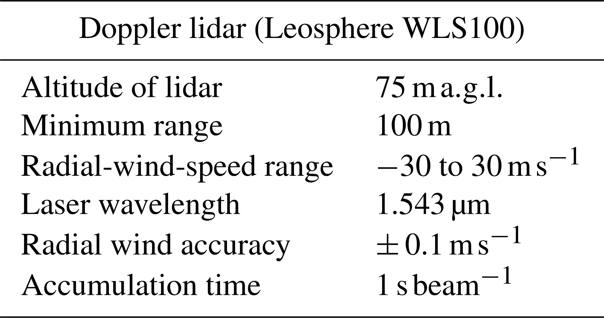
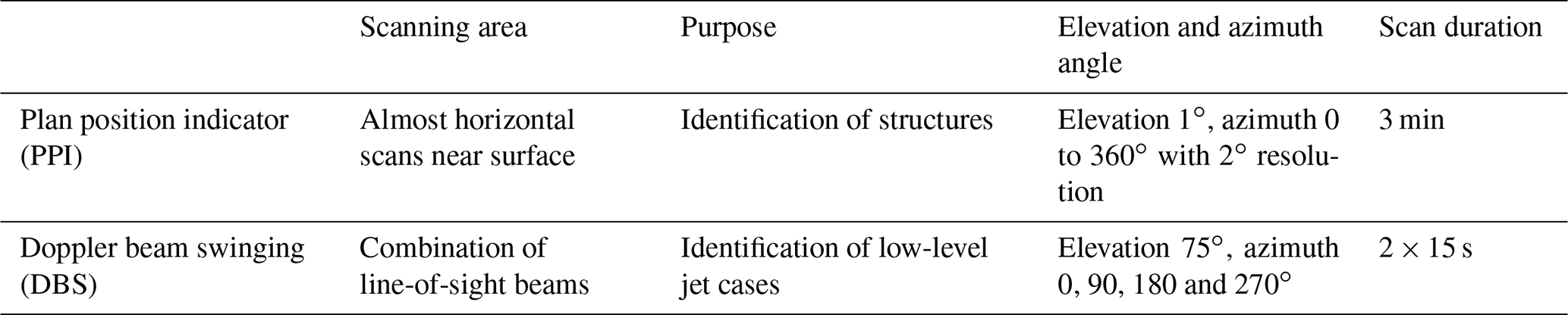
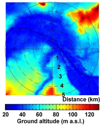
Figure 2 Ground altitude map above sea level with 75 m spatial resolution for the scanning area in Paris (credit: Institut National de l'Information Géographique et Forestière, https://www.data.gouv.fr/fr/datasets/bd-alti-r-75-m-250-m-1-000-m/, last access: 2 December 2020).

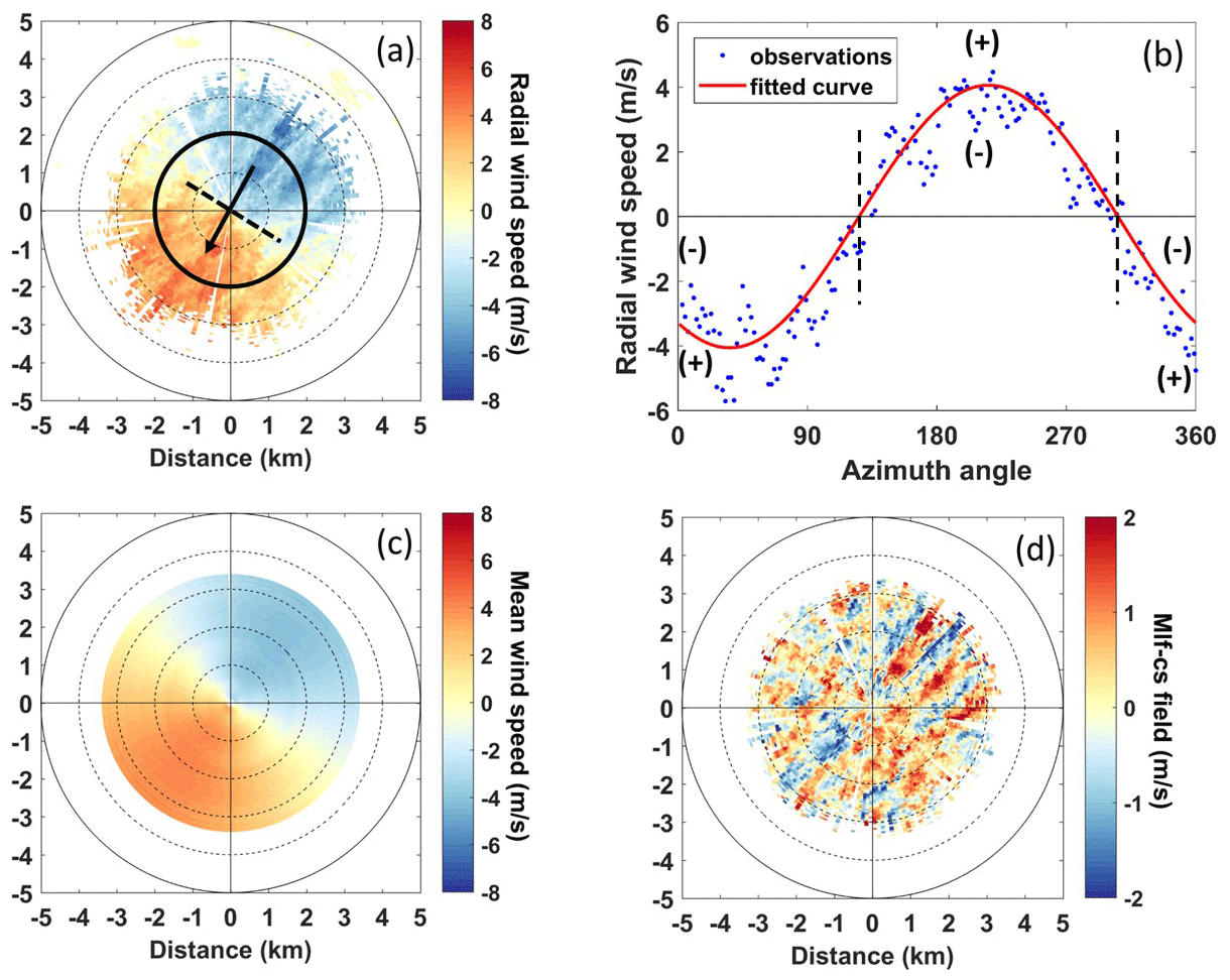
Figure 3 Observations recorded during a quasi-horizontal PPI scan on 8 September 2014 at the Jussieu site, Paris, at 09:26 UTC. (a) Radial wind speed along with the mean wind direction (black line) and the transverse direction perpendicular to it (black dotted line). (b) Radial wind speed (blue dots) as a function of the azimuth angle at a fixed 2 km distance from the lidar (black circle on a) along with the cosine fit function (red line). (c) Mean wind speed projected on the beam direction. (d) The mlf-cs field.

The Doppler shift frequency between the emitted laser beam and the light backscattered by the aerosols is measured by heterodyne detection associated with fast Fourier transform as explained analytically by Cariou et al. (2007). A wind lidar measures the radial wind speed, i.e. the wind projection along the light beam (counted positive when going away from the lidar). Table 2 showcases the implemented scanning methods during the VEGILOT campaign. For the classification of the mlf-cs's, we focused in the current study on the almost horizontal PPI scans (1^∘ elevation angle). During those scans, the lidar emitted beams in azimuth angles from 0 to 360^∘ with a 2^∘ resolution. This scenario was repeated every 18 min hence providing 4577 PPI scans during the whole campaign. The duration of each scan was 3 min, which is sufficiently fast for the observation of coherent structures with a lifespan of several minutes. The maximum range of the scans reached 5 km (see white circle of Fig. 1b) with a spatial resolution of 50 m. It is noteworthy that the scanning area covers almost exclusively the urban area of Paris, a city famous for regulating the height of the buildings to not exceed 50 m in its centre (Saint-Pierre et al., 2010). The ground altitude enclosed by the scanning area mostly ranges between 30 and 60 m with the exception of some hills near the boundaries of the scanning range as can be seen in Fig. 2. It is fundamental for this study to assume that the wind field within the scanning area is homogeneous (see Sect. 3.1). Due to the 1^∘ elevation, the beam was risen by about 87 m between the central point and the point at 5 km. It was also important for this study to retrieve observations regarding the vertical wind shear. For this purpose, the Doppler beam-swinging (DBS) scanning method was implemented. This method consisted of four line-of-sight beams at azimuth angles of 0, 90, 180 and 270^∘ with an elevation angle of 75^∘, and it was applied twice. The duration of the four beams emission was approximately 15 s.

3 Preparation of the dataset for the classification

3.1 Turbulent radial wind fields

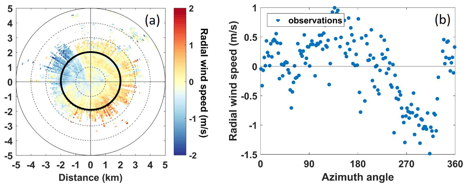
Figure 4 A case when the VAD method cannot be applied: (a) radial wind field on 25 September 2014 at 23:42 UTC and (b) radial wind speed (blue dots) as a function of the azimuth angle at a fixed 2 km distance from the lidar (black circle on a).

Assuming a homogeneous wind field for horizontal PPI scans, the radial-wind measurements u_r taken for the different beams at a given distance from the lidar should follow a cosine function of the azimuth angle, due to the projection of the wind along the beam direction (Eberhard et al., 1989). For instance, the observations at 2 km from the lidar (black ring in Fig. 3a) are displayed in Fig. 3b and can be fitted by a cosine function in the form of Eq. (1):

$$\begin{array}{}\text{(1)}& u_{\mathrm{r}}=a+b\cos (\mathit{\theta }-{\mathit{\theta }}_{max}),\end{array}$$

where b is the mean wind speed, θ_max is the wind direction, θ is the azimuth angle of the beam and a is the offset (Browning and Wexler, 1968; Lhermitte, 1962). It is noteworthy that the value of a is much smaller than b for our data. It is possible to retrieve the mean wind from all the “rings” and subsequently calculate the mean wind projected on the beam direction which is displayed in Fig. 3c. The difference between the radial wind field u_r (Fig. 3a) and the mean wind projected on the beam direction (Fig. 3c) is the mlf-cs of the radial wind field $u_{\mathrm{r}}^{\prime }$ (Fig. 3d), a parameter that indicates the existence of a turbulent atmosphere. For this study, the radial-wind-speed values for which the carrier-to-noise ratio is lower than −27 dB (CNR < −27 dB) were disregarded, since they were anomalously high, exceeding the values of the rest of the radial wind field by 2 times or more. Therefore the effective scanning range showcased in Fig. 3 is approximately 3 km. For a better visual representation of the patterns, the sign of the $u_{\mathrm{r}}^{\prime }$ in the current study is positive when the radial wind speed is stronger than the mean wind speed and negative when it is weaker as is illustrated in the sign convention of Fig. 3b, and it was computed by the following expression:

$$\begin{array}{}\text{(2)}& u_{\mathrm{r}}^{\prime }=\mathrm{|}{u}_{\mathrm{r}}\left(\mathit{\theta }\right)\mathrm{|}-\mathrm{|}f\left(\mathit{\theta }\right)\mathrm{|},\end{array}$$

where f is the fitted curve.

The Jussieu site is located in an urban area near hills; hence the surface roughness or the orography can affect the regional wind flow. Troude et al. (2002) and Lemonsu and Masson (2002) have performed numerical weather simulations in the area of Paris and have observed that during low-wind conditions (below 3 m s⁻¹) the orographic effect and the urban heat island effect could be the main drivers for the local wind speed. As a result, in some cases the radial wind field does not follow a cosine function, and therefore the VAD method cannot be applied. This is apparent especially at night when low winds (below 2 m s⁻¹) do not have a defined direction (Wilson et al., 1976). Figure 4 presents a case where the radial wind field is not homogeneous. The radial-wind-speed values e.g. at 2 km did not follow a cosine function (Fig. 4b).

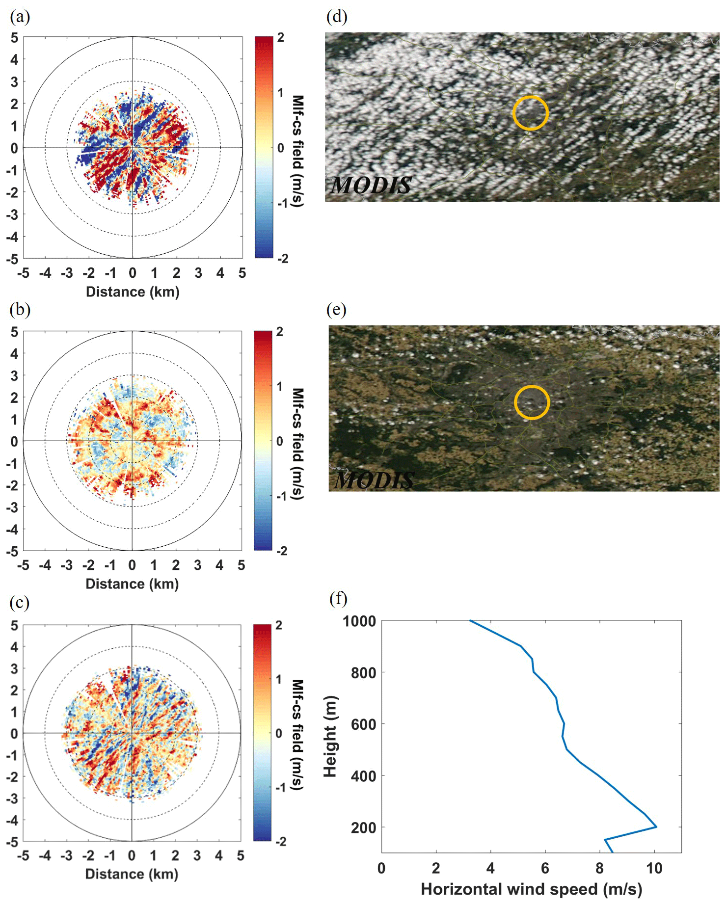
Figure 5 The upper part shows the three types of mlf-cs fields to classify: (a) rolls observed on 13 October 2014 at 12:52 UTC, (b) unaligned thermals observed on 16 September 2014 at 12:52 UTC and (c) streaks observed on 9 September 2014 at 20:49 UTC. The lower part shows the ancillary observations used to ascertain the structure type: (d) and (e) are true-colour images recorded by MODIS Aqua on the same day as (a) and (b) at 12:50 UTC, and (f) is the horizontal wind speed profile recorded by the Doppler lidar using the DBS technique on the same day as (c) at 20:51 UTC.

The visual examination of the mlf-cs fields led to the identification of three types of remarkable mlf-cs patterns. The first type was represented by large elongated areas of positive mlf-cs's accompanied by large elongated areas of negative mlf-cs's aligned with the mean wind (Fig. 5a) during the day. In the atmosphere, these types of patterns are encountered concurrently with the existence of rolls, where strong descending motions enhance the horizontal wind speed and ascending motions reduce it. The second type of pattern was characterized by large enclosed areas of a positive mlf-cs field attached to large enclosed areas of a negative mlf-cs field (Fig. 5b) during the day. The convergence zones formed between the positive and negative mlf-cs fields during unstable conditions (e.g. high solar radiation) are able to form strong unaligned thermals. Finally, the third type of pattern consisted of narrow elongated areas alternating between positive and negative mlf-cs's aligned with the mean wind (Fig. 5c). These patterns resemble turbulent streaks as described in Sect. 1.

In order to train the classification algorithm (Sect. 4.1), it was necessary to build an ensemble of cases for which the presence of rolls, unaligned thermals or streaks was confirmed by observations other than the lidar measurements. Moderate Resolution Imaging Spectroradiometer (MODIS) true-colour images were used to detect the presence of cloud streets over Paris (Fig. 5d), which confirmed the existence of rolls as stated in Sect. 1. Close to the moment when the cloud streets were present, rolls patterns were observed at the turbulent radial fields (Fig. 5a). It is noteworthy to mention that, for the training ensemble, we selected only cases of rolls occurring around the satellite overpass time to ensure the presence of cloud streets and thus the existence of rolls. However, for this classification we are interested in all the cases of rolls, with or without the formation of cloud streets. It is important to note that we observed the occurring patterns near the surface, hence near the lower part of the rolls. Regarding unaligned thermals, solar-radiation measurements from the meteorological station of Paris-Montsouris indicated the occasions when the hourly values were higher than the monthly average hourly values according to the Photovoltaic Geographical Information System (Huld et al., 2012), signifying fair-weather cumulus conditions. For approximately the same time of the day, we observe the unaligned thermals patterns. Figure 5b showcases an example of a turbulent radial wind field with unaligned thermals along with fair-weather cumuli over Paris as observed on MODIS true-colour images at approximately the same time (Fig. 5e).

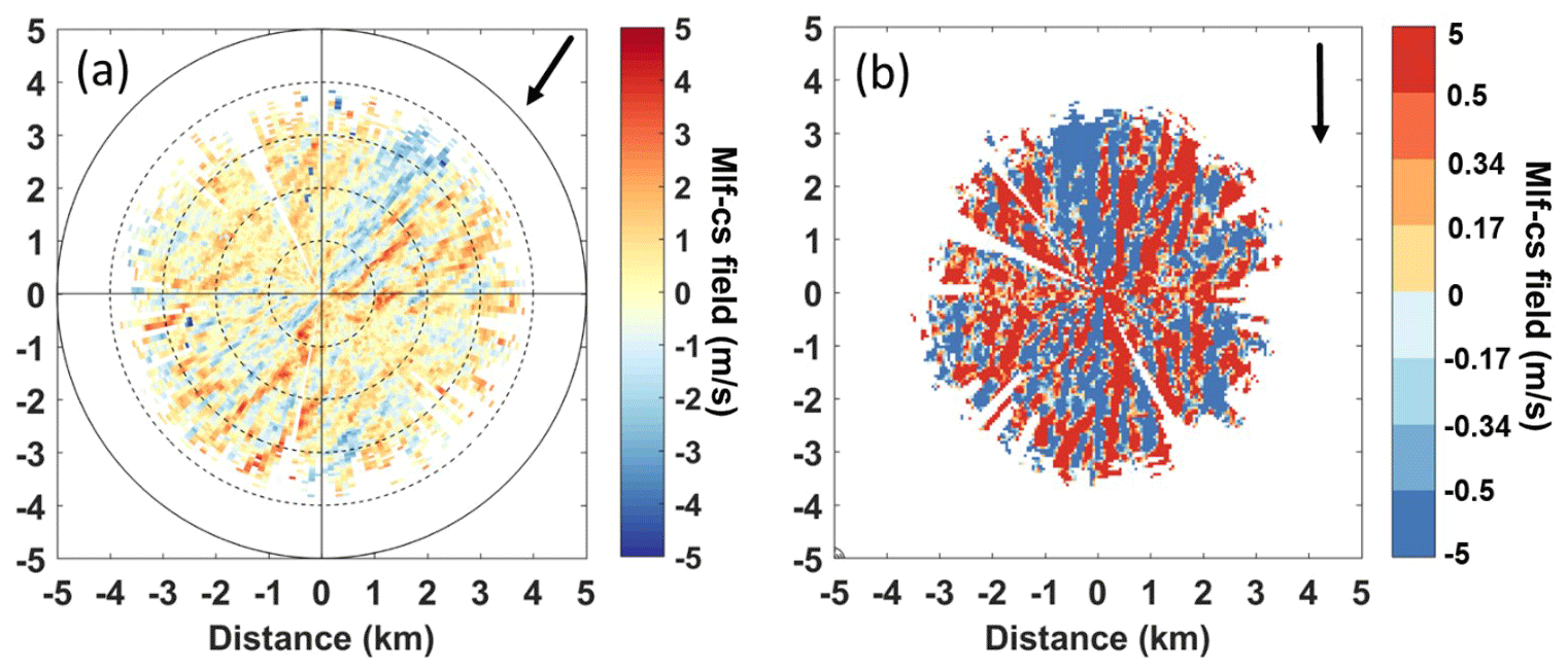
Figure 6 The mlf-cs field (a) before and (b) after image pre-processing with the arrow representing the mean wind direction on 10 September 2014 at 19:57 UTC.

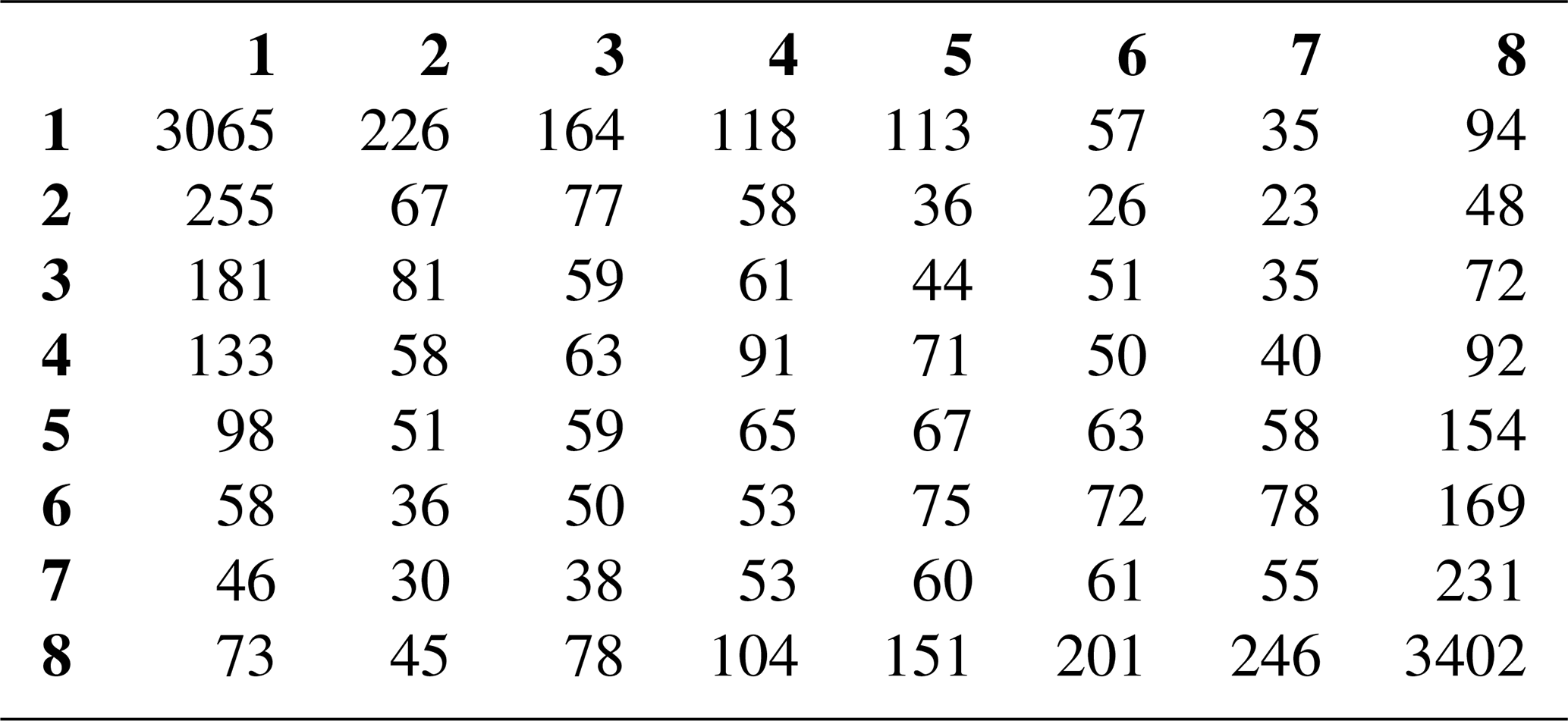
Table 3 Co-occurrence matrix after the image pre-processing (Fig. 6b) for the first neighbour (n=1) and for a cell pair aligned with the mean wind and oriented in the same direction (azimuth $\mathit{\phi }=\mathrm{0}{}^{\circ }$).

Finally concerning streaks, a driving factor for their formation is the existence of a strong wind shear near the surface. The observation of the horizontal wind profiles from the DBS scans revealed when the local maxima horizontal wind speed was higher than 2 m s⁻¹ compared to the local minima above it, which is defined as the threshold for nocturnal low-level jet events (Stull, 1988) (Fig. 5f). It is important to note that the location of the local maxima and minima of the horizontal wind speed were consistent during the study period, ranging from 200 to 300 and 400 to 500 m, respectively. The horizontal wind speed U_hor was estimated by the zonal u and meridional v winds via the expression

$$\begin{array}{}\text{(3)}& U_{\text{hor}}=\sqrt{u^{\mathrm{2}}+v^{\mathrm{2}}}.\end{array}$$

For the training ensemble, only night cases when streaks patterns (Fig. 5c) were accompanied by differences in local maxima and minima of the U_hor higher than 2 m s⁻¹ were selected. In total, 30 cases of each structure type were selected for the training ensemble with an extra category representing all the patterns that are not classified in the other three categories, such as chaotic patterns or cases when the VAD method cannot be applied (Fig. 4). Regarding rolls, streaks and thermals, only cases with symmetric radial wind fields were selected in order to ensure that the VAD method was applicable. The selection of symmetric radial wind fields was based on the visual examinations of the radial wind fields and the individual cosine function fits.

3.2 Computation of the co-occurrence matrices

In order to retrieve comparable texture analysis parameters from the mlf-cs field of the scans, the mlf-cs field was rotated so that the mean wind direction was aligned to the vertical (0^∘ corresponds to a wind blowing from the north). Then, the coordinates were converted from polar to Cartesian. It was also important to adjust the contrast of the image so that the difference between the areas of positive and negative turbulent wind speed became more prominent. For this purpose, the contrast of the images was increased by mapping the turbulent-wind-speed values into eight levels. One bin included all the negative values below −0.5 m s⁻¹; six bins were equally distributed between −0.5; and +0.5 m s⁻¹ and one bin included all the positive values above +0.5 m s⁻¹ (Fig. 6b).

For the automated classification of patterns, we need to map them to a space of corresponding numerical parameters. Each reconstructed mlf-cs field is represented by a matrix (cells corresponds to pixels) from which 8 × 8 co-occurrence matrices (CMs) can be constructed (Haralick et al., 1973). The rows and columns of the CM represent the wind levels from 1 to 8, whereas the cells contain the frequency of the combination of two neighbour pixels in the image. More specifically, the element at line i and column j contains the number of pixels with value i which are neighboured by pixels with value j. The first neighbour can be searched at different direction (e.g. left to right, top to bottom or diagonally) defining the cell pair orientation. In the same way a second, third, etc. neighbour can be selected. Thus, the CMs can be calculated for any cell pair orientations and neighbour order. CM were computed for various distances, i.e. neighbour orders n from 1 to 30 (distance from 50 m to 1.5 km), and all possible cell pair orientations, i.e. azimuth angles φ from −90^∘ (transverse direction from the mean wind in the anticlockwise direction) to +90^∘ (transverse direction in the clockwise direction). Table 3 shows the cell values of the CM built from the image of Fig. 6b for the first neighbour (n=1) and for a cell pair aligned with the mean wind and oriented in the same direction (azimuth $\mathit{\phi }=\mathrm{0}{}^{\circ }$). It is apparent that the vast majority of the occurrences are concentrated in the cells [1,1] and [8,8], as the structures are elongated and aligned with the mean wind direction.

Table 4 Co-occurrence matrix after the image pre-processing (Fig. 6b) for the third neighbour (n=3) and for the transverse direction in the clockwise direction (azimuth $\mathit{\phi }=+\mathrm{90}{}^{\circ }$).

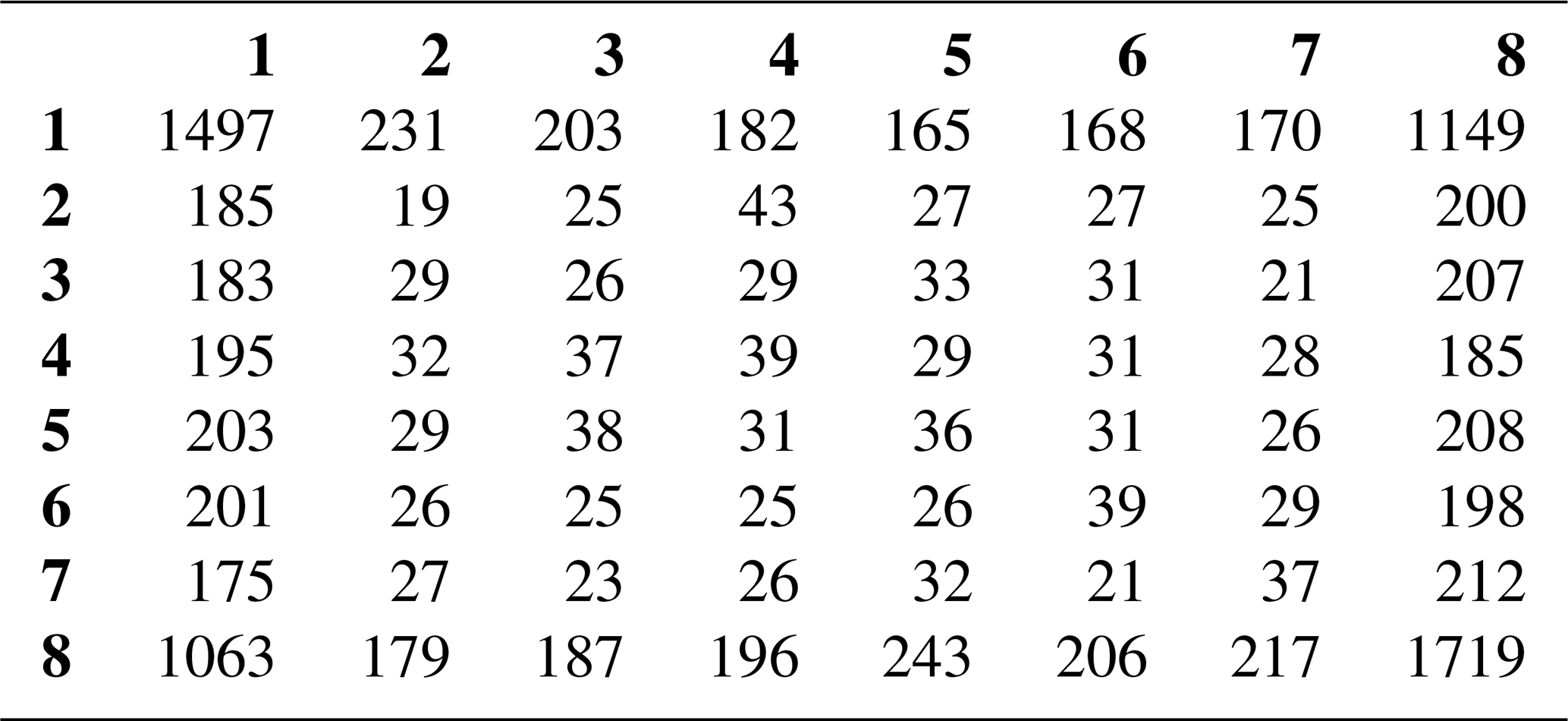
On the other hand, Table 4 shows the CM of Fig. 6b for the third neighbour (n=3) and for a cell pair oriented perpendicularly to the mean wind (transverse direction) with a clockwise rotation (azimuth angle $\mathit{\phi }=+\mathrm{90}{}^{\circ }$). In this case, the occurrences have been distributed to the cells [1,1] and [8,8], as well as to the cells [1,8] and [8,1]. As we can see in Fig. 6b, the structures alternate between positive and negative values in the direction transverse to the mean wind, thus creating this difference in the CM compared to Table 3.

3.3 Texture analysis parameters for the classification of the turbulent structures

It is possible to compute several texture analysis parameters from each CM. Srivastava et al. (2018) were able to distinguish different synthetic patterns by using four texture analysis parameters: correlation, contrast, homogeneity and energy. Correlation indicates the existence of linear structures in the image, with high values associated with a large amount of linear structure in the image. Contrast reveals the local variations in an image, where a large amount of variations leads to high values. Homogeneity is self-explanatory, and the high values represent a homogeneous image. Finally, energy measures the uniformity of an image with the highest values corresponding to constant or periodic forms (Haralick et al., 1973; Yang et al., 2012). In the study of Srivastava et al. (2018), the striped patterns resemble the elongated patterns of streaks and rolls that we observe in the turbulent radial wind field. Therefore, the same texture analysis parameters were selected for calculation in our dataset. More particularly, the following parameters were computed by Eqs. (4)–(7).

$$\begin{array}{}\text{(4)}& {\displaystyle }& {\displaystyle }\text{Homogeneity:}\text{Hom}\left(\mathit{\phi },n\right)=\sum _{i,j}{\displaystyle \frac{p(i,j)}{\mathrm{1}+\mathrm{|}i-j\mathrm{|}}},\text{(5)}& {\displaystyle }& {\displaystyle }\text{Contrast:}\text{Con}\left(\mathit{\phi },n\right)=\sum _{i,j}p(i,j)\mathrm{|}i-j{\mathrm{|}}^{\mathrm{2}},\text{(6)}& {\displaystyle }& {\displaystyle }\text{Correlation:}\text{Cor}\left(\mathit{\phi },n\right)=\sum _{i,j}{\displaystyle \frac{(i-{\mathit{\mu }}_i)(j-{\mathit{\mu }}_j)p(i,j)}{{\mathit{\sigma }}_i{\mathit{\sigma }}_j}},\text{(7)}& {\displaystyle }& {\displaystyle }\text{Energy:}\text{En}\left(\mathit{\phi },n\right)=\sum _{i,j}p(i,j{)}^{\mathrm{2}},\end{array}$$

where $p(i,j)=\frac{\text{CM}(i,j)}{\sum _{i,j}\text{CM}(i,j)}$ for the i,j position in the CM, marginal expectations ${\mathit{\mu }}_i=\sum _i\sum _{j}i\cdot p(i,j)$, ${\mathit{\mu }}_j=\sum _i\sum _{j}j\cdot p(i,j)$, and the marginal SDs ${\mathit{\sigma }}_i=\sqrt{\sum _i\sum _j(i-{\mathit{\mu }}_i{)}^{\mathrm{2}}\cdot p(i,j)}$ and ${\mathit{\sigma }}_j=\sqrt{\sum _i\sum _j(j-{\mathit{\mu }}_j{)}^{\mathrm{2}}\cdot p(i,j)}$.

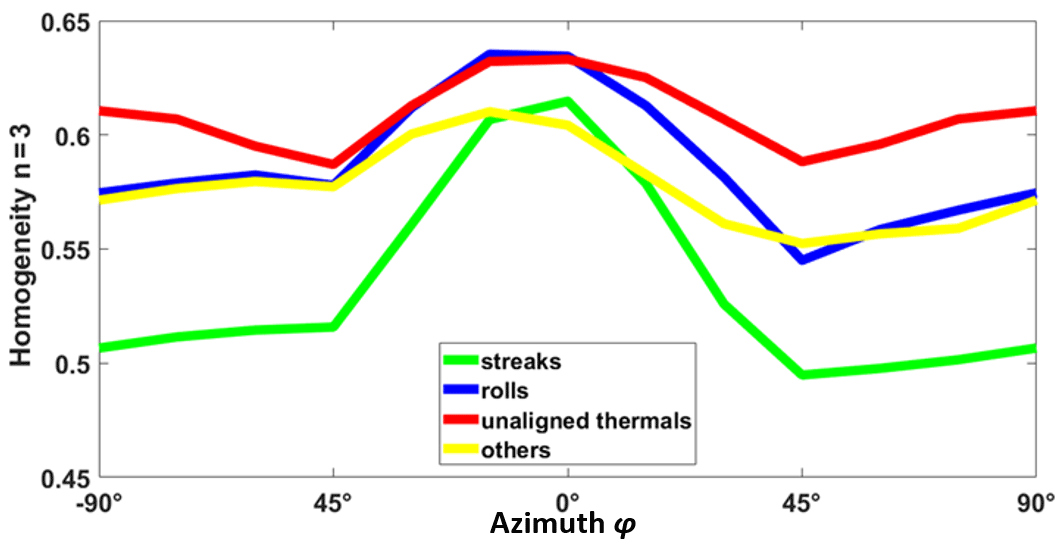
Figure 7 Third-neighbour homogeneity as a function of azimuth for one selected scan of each type.

At a given neighbour order n, it is then possible to study the dependence of the texture parameters to the azimuth angle φ (see an example of such a dependence in Fig. 7). The streaks and rolls have a more prominent peak in the longitudinal direction ($\mathit{\phi }=\mathrm{0}{}^{\circ }$) compared to the unaligned thermals and patterns of “others”. As streaks and rolls are aligned with the mean wind (azimuth $\mathit{\phi }=\mathrm{0}{}^{\circ }$), those peaks result from the elongated shapes of these patterns.

Three parameters of the curve in Fig. 7 were selected in order to distinguish the different types of structures. For instance, for the homogeneity curves, these parameters are defined as follows in Eqs. (8)–(10).

$$\begin{array}{}\text{(8)}& {\displaystyle }\begin{array}{rl}\text{Amplitude:}\text{Hom.Amp}\left(n\right)=& \underset{\mathit{\phi }}{max}\left(\text{Hom}(\mathit{\phi },n)\right)\\ & -\underset{\mathit{\phi }}{min}\left(\text{Hom}(\mathit{\phi },n)\right)\end{array}\text{(9)}& {\displaystyle }\text{Integral:}\text{Hom.Int}\left(n\right)=\sum _{\mathit{\phi }}\text{Hom}(\mathit{\phi },n)\text{(10)}& {\displaystyle }\begin{array}{rl}\text{Symmetry:}\text{Hom.Sym}\left(n\right)=& \sum _{\mathit{\phi }}\mathrm{|}\text{Hom}(\mathit{\phi },n)\\ & -\text{Hom}(-\mathit{\phi },n)\mathrm{|}\end{array}\end{array}$$

These three curve parameters were calculated for the 4 texture analysis parameters and for each of the 30 neighbour orders, which gives 360 parameters. In addition to these parameters, the time in UTC (close to solar time in Paris), the average mean wind speed and the root-mean-square error (RMSE) of the cosine fit (Fig. 3b) were included in the classification parameters. The total number of classification parameters associated with each scan was therefore 363.

4 Classification using supervised machine learning

4.1 Algorithm training and classification error

In order to classify the mlf-cs's according to the aforementioned texture analysis parameters, the supervised machine-learning methodology was applied (Bonamente, 2017; James et al., 2000; Kubat, 2017). The QDA algorithm was used, which minimizes the total probability of misclassification, assuming that features of each class have a multidimensional Gaussian distribution. QDA or normal Bayesian classification (Hastie et al., 2009) is the parametric approach implying that probability density functions (PDFs) belong to the family of normal distributions. It is a classical algorithm of supervised machine learning, based on the principle of maximum likelihood. The general idea is to estimate the PDF for each class and then select the most probable class (Kubat, 2017).

The greedy algorithm of stepwise forward selection was used in the article, which is the standard and frequently used method of reduction of the feature space. As indicated in Sokolov et al. (2020), it can be formulated as follows. The features are divided into two groups: accepted in the classification model and remaining, for which an estimate of the possibility of acceptance into the model is checked. Features from the set of “remains” are consecutively added to the model, and corresponding estimations of the classification error are calculated. From the received set of errors, the minimum is chosen and compared with the error of the previous model. If a significant reduction of the error occurred, then the corresponding feature is accepted into the model; if this is not true, then the process stops. The QDA was trained (Hastie et al., 2009; Sokolov et al., 2020) with the 150-case ensemble described in Sect. 3.1: 30 cases of streaks, 30 cases of rolls, 30 cases of unaligned thermals and 60 cases of others. The category of others was represented by twice as many cases, since it is expected to be the dominant category in the classification, as it includes the chaotic mlf-cs fields and the cases where the mlf-cs field was not computed successfully by the VAD method. The algorithm can be sensitive to an unbalanced training ensemble. Therefore, the selection of a training ensemble based on the expected results was preferred (Kubat, 2017).

The total omission error (see Sokolov et al., 2020) of the classification based on the QDA technique could be estimated for the training ensemble by means of 10-fold cross validation. This error is referred further as the classification error. In this method, the algorithm is trained using 90 % of the training ensemble (135 cases); it is then applied to the remaining 10 % (15 cases), and the resulting (output) classes are compared to the expected (target) classes. The process is repeated 10 times, each time extracting a different 10 % sample for testing, until the entire training ensemble has been tested.

Figure 8 Parameters selected to minimize the classification error of the training ensemble by the QDA method. From left to right: amplitude of the homogeneity for the 2nd neighbour, integral of the contrast for the 18th neighbour, amplitude of the contrast for the 4th neighbour, integral of the correlation of the 8th neighbour and symmetry of the homogeneity for the 2nd neighbour.

As the number of dimensions of the feature space (363) was significantly higher than the number of patterns of the training ensemble (150), the application of all the features leads to the curse of the dimensionality problem, when the classification works well only for the training data and fails for the test set. In order to deal with this problem, we reduced the feature space by selecting the most informative components using the stepwise forward-selection algorithm (Sokolov et al., 2020). The resulting sequence of these components and the decrease of the 10-fold cross-validation classification error are presented in Fig. 8. The classification error reached a minimum of about 9.2 % when five parameters were used; taking more into account increased the classification error.

Analytically, these parameters are the amplitude of the 2nd-neighbour homogeneity curve, the integral of the 18th-neighbour contrast curve, the amplitude of the 4th-neighbour contrast curve, the integral of the 8th-neighbour correlation curve and the symmetry of the 2nd-neighbour homogeneity curve. These results show that the prominent peaks are a distinctive characteristic for the elongated patterns, as the amplitude of the homogeneity and contrast curves are two of the significant parameters. Furthermore, the integral or more precisely the sum of the points of the curves for the contrast and for the correlation curves are significant parameters as well. This is important especially for the distinction between the categories thermals and others, as their amplitude may not differ substantially, since the patterns are not towards a specific direction, yet a chaotic area will have higher values of contrast and lower values of correlation compared to an enclosed homogeneous area. Finally, the symmetry of the homogeneity curve as a classifier reveals the urgency to align the turbulent radial wind fields to the mean wind direction and thus align the structures such as streaks and rolls with the mean wind direction in order to be distinguishable from the random positions of the enclosed structures of the thermals or the chaotic structures of others. It is also crucial to note that the parameters cover various distances, from the 2nd neighbour, which in grid points is 100 m, to the 18th neighbour, which is 900 m. This is necessary for our classification, since streaks and rolls are both elongated patterns, but their transverse horizontal sizes differ. Furthermore, it demonstrates the ability of the algorithm to distinguish structures with different sizes. It is noteworthy that the curve parameters play a more significant role in the classification of the structures in comparison to time, mean wind field and cosine fit RMSE.

Table 5 Confusion matrix calculated for the training dataset. The “target class” corresponds to the visual classification, while the “output class” corresponds to the class attributed by the algorithm. Therefore, the cells in the “roll” column, for instance, give the number of roll cases that were classified properly (roll line) or improperly (other lines) in the different categories.

The detailed results of the cross validation of the QDA classification for the algorithm with five predictors are displayed in Table 5. The algorithm allowed for classifying correctly about 91 % of the training ensemble. The algorithm performs the most precise classification for the streaks with a classification error of only 3.3 %, as one case was misclassified as rolls. Regarding the category of others, the results are equivalently accurate with a classification error of 3.3 %, as two cases were misclassified as thermals. Moreover, the performance of the algorithm for rolls was good with a classification error of 10 % with three cases being misclassified as thermals. Thermals were the most troublesome type for classification by the algorithm; the algorithm classified correctly 24 cases. Four cases were misclassified as rolls, and two cases were misclassified as others, showing a classification error of 20 %.

4.2 Results of the trained algorithm over the 2-month dataset

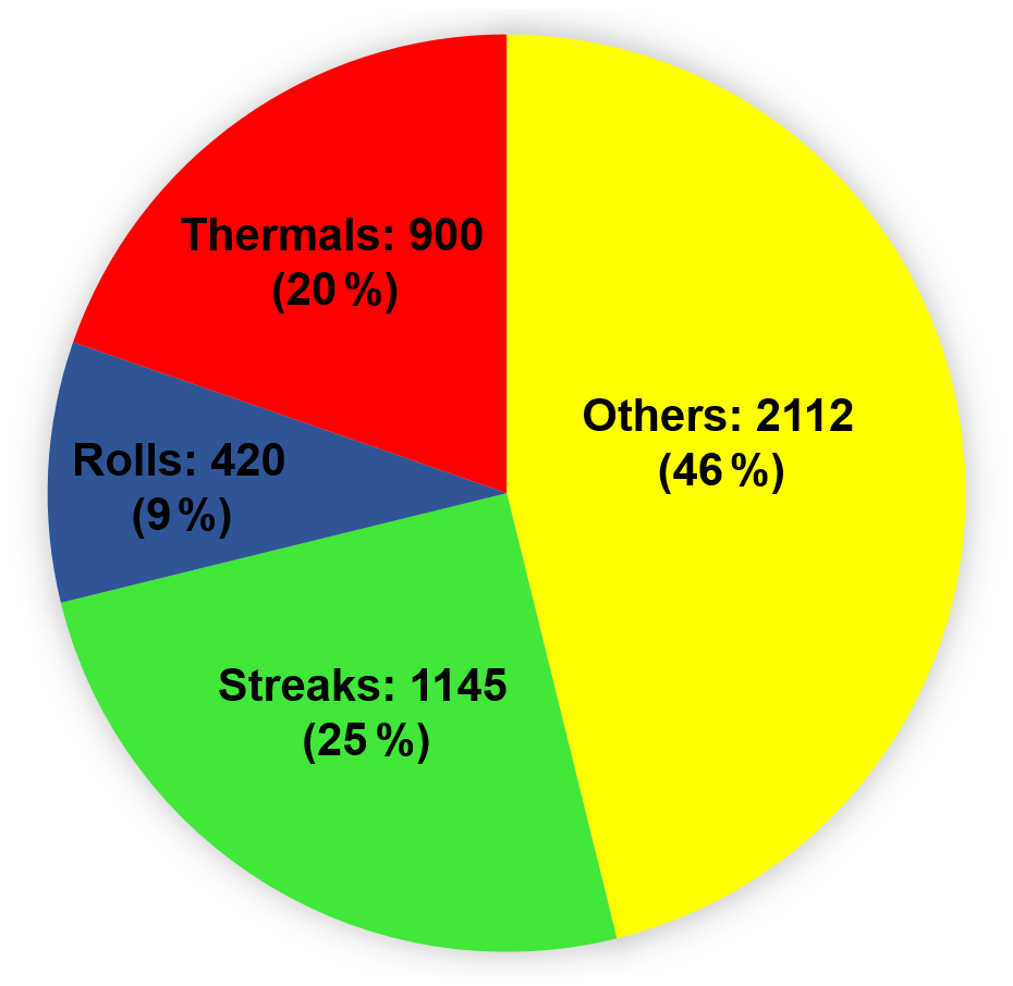
Figure 9 Classification of the whole ensemble using the QDA method according to the parameters of Fig. 8.

The whole dataset, consisting of 4577 scans, was classified according to the five parameters showcased in Fig. 8. The results are displayed in Fig. 9.

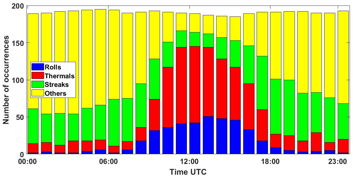
Figure 10 Histogram of the number of occurrences of the different types of structures with respect to time in UTC.

The algorithm classifies 54 % of the 2-month dataset as containing mlf-cs's and 34 % in particular as coherent structures (streaks and rolls). The most frequent cases of mlf-cs's were streaks (25 %), and the least frequent cases were rolls (9 %). It is important to note that, in our classification, we considered only thermals and rolls during daytime. Figure 10 illustrates the number of occurrences for each type of structure at a particular time of the day during the 2 months of the campaign. It is evident that despite time not being one of the selected classifiers, the number of occurrences of the structures shows a distribution that can be associated with the atmospheric conditions. More particularly, rolls and thermals were mainly classified during the day. This result is noteworthy, as these structures are linked to a well-developed atmospheric boundary layer during the day. On the contrary, there were scarcely any roll cases observed at night, and a few unaligned thermals were classified at night. This stems from the training process, where some cases of thermal were improperly classified as others and the reverse. Regarding the cases of others, these were mostly observed during the night. This was expected, since the cases of low winds with no defined direction – when the VAD method cannot be applied – occur mainly during the night. We also see that streaks were observed more frequently during the night, when mechanical turbulence becomes dominant. This was also expected as the nocturnal low-level jets are a main driving force for the formation of streaks, and we observed the occurrence of the local maxima of the horizontal wind speed near the surface higher than 2 m s⁻¹ compared to the local minima over Paris for 20 out of the 62 nights during the VEGILOT campaign.

5 Conclusions

The current study showcases that it is possible to identify and classify mlf-cs's such as streaks, rolls and unaligned thermals with horizontal scans from a single Doppler lidar by combining texture analysis parameters and the QDA supervised machine-learning technique. By applying the VAD method to the radial-wind observations, it is possible to identify mlf-cs's that can be distinguished as narrow elongated (streaks), wide elongated (rolls), large enclosed (thermals) and chaotic (others) patterns. The diversity of the patterns was also depicted in the curves of the texture analysis parameters with the elongated patterns (streaks and rolls) showing a prominent peak compared to more chaotic or enclosed patterns (unaligned thermals).

A training ensemble of 150 cases was selected by combining visual examination of the patterns and studying characteristic physical properties corresponding to streaks, rolls and unaligned thermals. Subsequently, the QDA algorithm with stepwise forward selection of the features was applied to the training ensemble, and its performance was estimated using the cross-validation technique. The results showed a successful classification for 91 % of the training ensemble using five texture analysis parameters as predictors. More particularly, these parameters were the amplitude of the 2nd-neighbour homogeneity curve and the amplitude of the 4th-neighbour contrast curve which were associated with the prominent peaks of the elongated patterns (streaks and rolls). Furthermore, the integral of the 18th-neighbour contrast curve and the integral of the 8th-neighbour correlation curve which could distinguish, for example, chaotic patterns (others) with high contrast and lower values of correlation between neighbour points compared to an enclosed homogeneous type (thermals). Finally, the symmetry of the 2nd-neighbour homogeneity curve revealed the importance to align the mlf-cs fields to the mean wind direction. Another striking outcome of the QDA classification was the variety of the classifiers in terms of distance between the grid points. The 2nd neighbour translates in a distance between two grid points equivalent to 100 m, and for the 18th neighbour this is 900 m. This is essential for the classification between patterns with different sizes such as streaks and rolls. The algorithm performed best for the category of streaks with a classification error of only 3.3 %. Time, mean wind speed and the cosine fit RMSE of the VAD method were not selected by the algorithm for the classification.

The whole ensemble of the 4577 scans was classified by the trained QDA algorithm using the five selected texture analysis parameters. The results showed that 54 % of cases were classified as mlf-cs's, among which 34 % were coherent structures (streaks and rolls). The streaks were mostly observed during night, whereas the thermals and rolls were almost exclusively observed during the day, with only a few cases classified between sunset and sunrise. The classified ensemble can be used for statistical studies of the mlf-cs physical parameters, such as structure size, as a function of weather conditions (PBL height, temperature, wind speed, radiation, etc.). Moreover, the development of the structures can be analysed and comprehended.