Effects of the prewhitening method, the time granularity, and the time segmentation on the Mann–Kendall trend detection and the associated Sen's slope

The Mann–Kendall test associated with the Sen's slope is a very widely used non-parametric method for trend analysis. It requires serially uncorrelated time series, yet most of the atmospheric processes exhibit positive autocorrelation. Several prewhitening methods have therefore been designed to overcome the presence of lag-1 autocorrelation. These include a prewhitening, a detrending and/or a correction of the detrended slope and the original variance of the time series. The choice of which prewhitening method and temporal segmentation to apply has consequences for the statistical significance, the value of the slope and of the confidence limits. Here, the effects of various prewhitening methods are analyzed for seven time series comprising in situ aerosol measurements (scattering coefficient, absorption coefficient, number concentration and aerosol optical depth), Raman lidar water vapor mixing ratio, as well as tropopause and zero-degree temperature levels measured by radio-sounding. These time series are characterized by a broad variety of distributions, ranges and lag-1 autocorrelation values and vary in length between 10 and 60 years. A common way to work around the autocorrelation problem is to decrease it by averaging the data over longer time intervals than in the original time series. Thus, the second focus of this study evaluates the effect of time granularity on long-term trend analysis. Finally, a new algorithm involving three prewhitening methods is proposed in order to maximize the power of the test, to minimize the number of erroneous detected trends in the absence of a real trend and to ensure the best slope estimate for the considered length of the time series.

1 Introduction

To estimate climate changes and to validate climatic models, long-term time series associated with statistically adapted trend analysis tools are necessary. The basic requirements needed to apply specific statistical tools are usually well described, but end-users often do not systematically test whether the properties of their time series fulfill these requirements. An inappropriate usage of the statistical tools may lead to misleading conclusions. It may also happen that a time series does not meet the complete criteria of any of the statistical tools. In that case, the statistical tool must be adapted or different methods with complementary strengths and weaknesses must be used.

The time series properties that can cause misuse of statistical tools for trend analysis primarily concern the statistical distribution, the autocorrelation, missing data or periods without measurements, the presence of seasonality, irregular sampling, the presence of negatives and the rules applied in the case of data below-detection limits. A large number of trend analysis tools such as the whole family of least mean square and generalized least square methods are parametric methods and, consequently, require normally distributed residues. Unfortunately, many atmospheric measurements, which strongly depart from the normal distribution, do not meet this requirement, so that non-parametric methods have to be used. Non-parametric techniques are commonly based on rank and assume continuous monotonic increasing or decreasing trends. The Mann–Kendall (MK) test associated with the Sen's slope is the most widely applied non-parametric trend analysis method in atmospheric and hydrologic research (Gilbert, 1987; Sirois, 1998). While it has no requirement for data distribution, it must be applied to serially independent and identically distributed variables. The second condition of homogeneity of distribution is not met if a seasonality is present, but it can be solved by using the seasonal Mann–Kendall test developed by Hirsch et al. (1982). The first condition of independence is not met if the data are autocorrelated, which is often the case for atmospheric variables that are controlled by autocorrelated physical or chemical processes. To correctly analyze autocorrelated and not normally distributed errors, two different strategies are usually applied.

The first strategy tends to decrease the amount of autocorrelation by aggregating time series into monthly, seasonal, or yearly bins or even into longer periods. However, coarser time granularities (e.g., due to longer averaging periods) do not ensure that autocorrelation is removed. Moreover, the aggregation implies a decrease in the information density in the time series, such as the diurnal or seasonal cycles, the variance of the data and to some extent the data distribution. The aggregation conditions (length of the time unit, making the time unit consistent with the observed seasonality, starting phase of the time series and the averaging method) may influence the trend results (de Jong and de Bruin, 2012; Maurya, 2013) in what is called the modifiable temporal unit problem (MTUP).

The second strategy focuses on the development of algorithms to reduce the impact of the autocorrelation artifacts on the statistical significance of the MK test and on the Sen's slope. Two kinds of algorithms are usually used: (i) the prewhitening of the data to remove the autocorrelation and (ii) inflation of the variance of the trend test statistic to take into account the number of independent measurements instead of the number of data points (the autocorrelation reduces the number of degrees of freedom in tests).

In this study, the effects of various prewhitening methods on the MK statistical significance and on the slope are analyzed for time series of in situ aerosol properties, aerosol optical depth, temperature levels (tropopause and zero-degree temperature levels) and remote sensing water vapor mixing ratios. This study also analyzes the effect of the time granularity on the MK statistical significance, on the strength of the slope and on the confidence limits of various atmospheric compounds for the atmospheric time series listed above. Additionally, a new methodology combining three prewhitening methods and called 3PW is proposed in order to handle correctly the autocorrelation without decreasing the power of the test while still computing the correct slope value.

2 The Mann–Kendall methodology (prewhitening methods)

The MK test for trends is a non-parametric method based on rank. The calculated S statistic is normally distributed for a number of observations N>10 and the significance of the trends is tested by comparing the standardized test statistic $Z=S/\left[\text{var}\right(S){]}^{\mathrm{0.5}}$ with the standard normal variate at the desired significance level. For N≤10, an exact S distribution has to be applied (see, e.g., Gilbert, 1987). Hirsch et al. (1982) extend the Mann–Kendall test to take seasonality in the data into account as well as the existence of multiple observations for each season. A global or yearly trend can be considered only if the seasonal trends are homogeneous at the desired confidence level (Gilbert, 1987). Confidence limits (CLs) are defined as the $\mathrm{100}\times (\mathrm{1}-p)$ percentiles of the standard normal distribution of all the pairwise slopes computed during the Sen's slope estimator, where p is the chosen confidence limit.

2.1 The problem of the autocorrelation in the MK test

The MK test determines the validity of the null hypothesis H₀ of the absence of a trend against the alternative hypothesis H₁ of the existence of a monotonic continuous trend. While no assumptions are needed about the data distribution (i.e., the definition of a non-parametric test), the MK test does require that the data are serially independent, namely the absence of autocorrelation in the time series. Statistical tests are prone to two types of error. The first is an incorrect rejection of the null hypothesis H₀ (a “type 1 error”). This error is related to an erroneously high statistical significance leading to false positive cases. The second is an incorrect acceptance of the null hypothesis H₀ (a “type 2 error”). This error can be understood as the power of the test being too low, leading to false negative cases.

The adverse effect of positive autocorrelation in time series on the number of type 1 errors was suggested by Tiao et al. (1990) and Hamed and Rao (1998) and later simulated (Kulkarni and von Storch, 1995; Zhang and Zwiers, 2004; Blain, 2013; Wang et al., 2015a, b; Hardison et al., 2019). All these studies clearly showed that positive autocorrelation in time series significantly increases the number of type 1 errors, whereas prewhitening procedures increase the number of type 2 errors. Larger lag-1 autocorrelation (ak₁) leads to a higher percentage of type 1 errors and to a larger bias in the Sen's slope. Zwang and Zwiers (2004) also show that the occurrence of both types of errors largely depends on the length of the time series, with longer periods leading to a strong reduction of errors and to a lower bias in the trend slope estimation.

A popular solution to get rid of the autocorrelation problem in the MK test is to aggregate the time series in order to decrease ak₁. While the use of coarse time granularity effectively decreases the autocorrelation, the suppression of autocorrelation is not guaranteed, even in monthly or yearly aggregations. Moreover, aggregation greatly decreases the number of observations N and can potentially affect the MK-test errors, the slope biases and the CLs.

Two kinds of statistical procedures were developed to correct the MK test for autocorrelation in the data. The variance correction approaches (Hamed and Rao, 1998; Yue and Wang, 2004; Hamed, 2009; Blain, 2013) consider inflating the variance of the S statistic so that the number of independent observations instead of the total number of observations is taken into account. These approaches appear to preserve the pre-assigned significance level and the power of the MK test in the absence of trend but not in the case of correlated time series and in the presence of a trend (Yue et al., 2002; Blain, 2013). The prewhitening approaches consider removing the lag-1 autoregressive (AR(1)) process in the time series prior to applying the MK test. Several algorithms with various strengths and disadvantages have been published and are described in the next section. Since negative autocorrelations are rare in atmospheric processes, only positive autocorrelations are taken into account in this study. Several studies have shown that the prewhitening methods are also applicable in the case of negative serial correlations but with dissimilar consequences (Rivard and Vigneault, 2009; Yue and Wang, 2002; Bayazit et al., 2004; Wang et al., 2015b).

2.2 The prewhitening methods

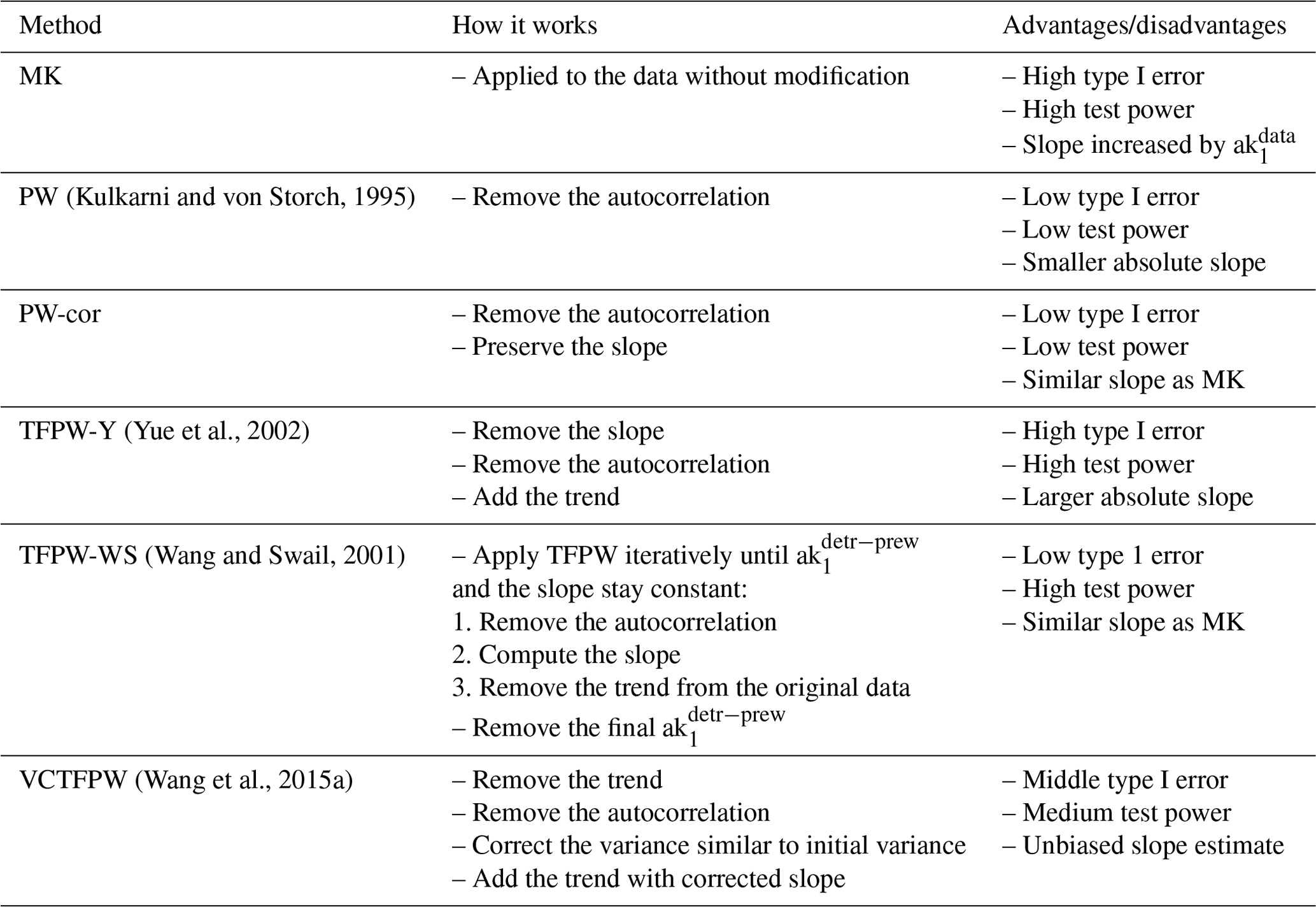
This section describes all the prewhitening methods known to the authors. The advantages and disadvantages of each method are summarized in Table 1. It has to be noted that, for all the methods proposed, the prewhitening can be applied only if ak₁ is statistically significant (ss) following a normal distribution at the two-sided 95 % confidence interval. The first implemented prewhitening method (hereafter called PW) simply removes the lag-1 autocorrelation ${\text{ak}}_{\mathrm{1}}^{\mathrm{data}}$ from the original data X at the time t:

$$\begin{array}{}\text{(1)}& X_t^{\mathrm{PW}}=X_t-{\text{ak}}_{\mathrm{1}}^{\mathrm{data}}{X}_{t-\mathrm{1}}.\end{array}$$

This PW method results in a low amount of type 1 errors, but the existence of real trends, either positive or negative, can lead to an overestimation/underestimation of ${\text{ak}}_{\mathrm{1}}^{\mathrm{data}}$, which will reduce the power of the test. A further procedure called trend-free prewhitening (TFPW) consists of removing the autocorrelation on detrended data. Yue et al. (2002) published the most commonly used method that consists of (i) estimating the Sen's slope β^data on the original data; (ii) removing the trend to obtain a detrended time series A^detr (Eq. 2); (iii) removing the lag-1 autocorrelation ${\text{ak}}_{\mathrm{1}}^{\mathrm{detr}}$ on A^detr to generate a detrended prewhitened time series A^detr−prew (Eq. 3); and (iv) adding the trend back in to generate the processed time series to evaluate (i.e., $X_t^{\mathrm{TFPW}-\mathrm{Y}}$) (Eq. 4):

$$\begin{array}{}\text{(2)}& {\displaystyle }& {\displaystyle }{A}_t^{\mathrm{detr}}=X_t-{\mathit{\beta }}^{\mathrm{data}}t,\text{(3)}& {\displaystyle }& {\displaystyle }{A}_t^{\mathrm{detr}-\mathrm{prew}}=A_t^{\mathrm{detr}}-{\text{ak}}_{\mathrm{1}}^{\mathrm{detr}}{A}_{t-\mathrm{1}}^{\mathrm{detr}},\text{(4)}& {\displaystyle }& {\displaystyle }{X}_t^{\mathrm{TFPW}-\mathrm{Y}}=A_t^{\mathrm{detr}-\mathrm{prew}}+{\mathit{\beta }}^{\mathrm{data}}t.\end{array}$$

This approach is called trend-free prewhitening (TFPW-Y) and restores the power of the test, albeit at the expense of an increase in type 1 errors. The original idea of Wang and Swail's (2001) was intended to implement the MK test on the prewhitened series rather than on the prewhitened detrended series, as was given by Eq. (8). If the prewhitened series are detrended, then trends will not be identified. Wang and Swail (2001) propose an iterative TFPW method to mitigate the adverse effect of the trend on the accuracy of the lag-1 autocorrelation estimate. This iterative procedure consists of (i) removing ${\text{ak}}_{\mathrm{1}}^{\mathrm{data}}$ from the original time series and correcting the prewhitened data for the modified mean (Eq. 5); (ii) estimating the Sen's slope β^prew on the prewhitened data $A_{\mathrm{cor},t}^{\mathrm{prew}}$; (iii) removing the trend (β^prew) estimated on the PW data from the original data to obtain a prewhitened detrended time series $A_{\mathrm{cor},t}^{\mathrm{detr}}$ (Eq. 6); and (iv) applying iteratively (i)–(iii) until the ak₁ and slope differences become smaller than a proposed tiny threshold of 0.0001 (Eq. 7).

$$\begin{array}{}\text{(5)}& {\displaystyle }{A}_{\mathrm{cor},t}^{\mathrm{prew}}=X_t^{\mathrm{PW}-\mathrm{cor}}=\left(X_t-{\text{ak}}_{\mathrm{1}}^{\mathrm{data}}{X}_{t-\mathrm{1}}\right)/\left(\mathrm{1}-{\text{ak}}_{\mathrm{1}}^{\mathrm{data}}\right),\text{(6)}& {\displaystyle }{A}_{\mathrm{cor},t}^{\mathrm{detr}}=\left(X_t-{\mathit{\beta }}^{\mathrm{prew}}t\right),\text{(7)}& {\displaystyle }\begin{array}{rl}& A_{\mathrm{cor},t}^{\mathrm{detr}-\mathrm{prew}}\\ & =\left(A_{\mathrm{cor},t}^{\mathrm{detr}}-{\text{ak}}_{\mathrm{1}}^{\mathrm{detr}-\mathrm{prew}}{A}_{\mathrm{cor},t-\mathrm{1}}^{\mathrm{detr}}\right)/\left(\mathrm{1}-{\text{ak}}_{\mathrm{1}}^{\mathrm{detr}-\mathrm{prew}}\right),\end{array}\text{(8)}& {\displaystyle }{X}_t^{\mathrm{TFPW}-\mathrm{WS}}=A_{\mathrm{cor},t}^{\mathrm{detr}-\mathrm{prew}},\end{array}$$

after n iterations until ${\text{ak}}_{\mathrm{1}}^{\mathrm{detr}-\mathrm{prew},n-\mathrm{1}}-{\text{ak}}_{\mathrm{1}}^{\mathrm{detr}-\mathrm{prew},n}<\mathrm{0.0001}$ and ${\mathit{\beta }}^{\mathrm{prew},n-\mathrm{1}}-{\mathit{\beta }}^{\mathrm{prew},n}<\mathrm{0.0001}$. Note that the use of a higher threshold up to 0.05 does not significantly modify the results obtained on the considered time series.

Table 1 Advantages and disadvantages of the MK test and of the various prewhitening methods.

Wang and Swail's (2001) TFPW method (TFPW-WS) restores the low number of type 1 errors without decreasing the power of the test (Zhang and Zwiers, 2004). The factor $(\mathrm{1}-{\text{ak}}_{\mathrm{1}}^{\mathrm{detr}-\mathrm{prew}}{)}^{-\mathrm{1}}$ is needed to ensure that the prewhitened time series possesses the same trend as the original time series. The preliminary step of the first iteration in the TFPW-WS method (removing ${\text{ak}}_{\mathrm{1}}^{\mathrm{data}}$ from the original time series and correcting the prewhitened data for the modified mean Eq. 5) corresponds to the standard PW method but with the same correction factor, ensuring a similar trend between the prewhitened and original time series. This method called PW-cor is, to the knowledge of the authors, not referenced in the literature but is a potential method tested in this study.

Finally, Wang et al. (2015a) proposed a further approach in order to correct TFPW-Y for both the elevated variance of slope estimators and for the decreased slope caused by the prewhitening. Practically, the variance of A^detr−prew (i.e., ${\mathit{\sigma }}_A^{\mathrm{2}}$) is restored to the variance of X (i.e., ${\mathit{\sigma }}_X^{\mathrm{2}}$) to generate the $A_{\mathrm{VC}}^{\mathrm{detr}-\mathrm{prew}}$ time series:

$$\begin{array}{}\text{(9)}& A_{\mathrm{VC},t}^{\mathrm{detr}-\mathrm{prew}}=A_t^{\mathrm{detr}-\mathrm{prew}}\cdot {\displaystyle \frac{{\mathit{\sigma }}_X^{\mathrm{2}}}{{\mathit{\sigma }}_A^{\mathrm{2}}}}.\end{array}$$

The slope estimator β^data is decreased in the case of positive autocorrelation by the square root of the variance inflation factor (VIF) to obtain the corrected slope ${\mathit{\beta }}_{\mathrm{VC}}^{\mathrm{detr}}$ (Eq. 11). Matalas and Sankarasubramanian (2003) provided a simple way to compute the limiting values of VIF for a sufficiently large sample size and a first-order autocorrelation:

$$\begin{array}{}\text{(10)}& \text{VIF}\approx \left(\mathrm{1}+{\text{ak}}_{\mathrm{1}}^{\mathrm{detr}}\right)/\left(\mathrm{1}-{\text{ak}}_{\mathrm{1}}^{\mathrm{detr}}\right),\end{array}$$

so that

$$\begin{array}{}\text{(11)}& {\mathit{\beta }}_{\mathrm{VC}}^{\mathrm{detr}}={\mathit{\beta }}^{\mathrm{data}}/\sqrt{\left(\mathrm{1}+{\text{ak}}_{\mathrm{1}}^{\mathrm{detr}}\right)/\left(\mathrm{1}-{\text{ak}}_{\mathrm{1}}^{\mathrm{detr}}\right)}\end{array}$$

and

$$\begin{array}{}\text{(12)}& X_t^{\mathrm{VCTFPW}}=A_{\mathrm{VC},t}^{\mathrm{detr}-\mathrm{prew}}+{\mathit{\beta }}_{\mathrm{VC}}^{\mathrm{detr}}t.\end{array}$$

Statistical simulations by Wang et al. (2015a) showed that this new variance-corrected prewhitening method (VCTFPW) leads to more accurate slope estimators, tends to mitigate the inflationary type 1 errors raised by autocorrelation and preserves to some extent the power of the test.

2.3 A new algorithm (3PW) involving three prewhitening methods

As described in Sect. 2.2 and Table 1, each of the presented prewhitening methods has a specific advantage: the low sensitivity to type 1 errors for PW, the high-test power for TFPW-Y, and the unbiased slope estimate for VCTFPW. TFPW-WS has both a low type 1 error and a high test power but requires more computing time due to the iteration process. Here, we propose a new algorithm (3PW), described in Fig. 1, which combines the advantages of each prewhitening method:

• -

  The ${\text{ak}}_{\mathrm{1}}^{\mathrm{data}}$ of the original time series is calculated. If it is not ss, the MK test is applied to the original time series. If ${\text{ak}}_{\mathrm{1}}^{\mathrm{data}}$ is ss, PW, TFPW-Y and VCTFPW are applied in order to obtain three prewhitened time series that are thereafter named after the specific prewhitening method for purposes of clarity.

• -

  The MK test that defines the statistical significance is applied to the PW and TFPW-Y data. If both tests are ss or not ss, the trend is considered ss or not ss, respectively. If TFPW-Y is ss but not PW, the trend is considered a TFPW-Y false positive (due to the higher sensitivity to type 1 errors of TFPW-Y) and the trend has to be considered not ss. If PW is ss but TFPW-Y is not, then the trend is considered a PW false positive and the trend has to be considered not ss. The probability P for the statistical significance is given by the higher probability between PW and TFPW-Y.

• -

  The Sen's slope is then computed on the VCTFPW data in order to have an unbiased slope estimate.

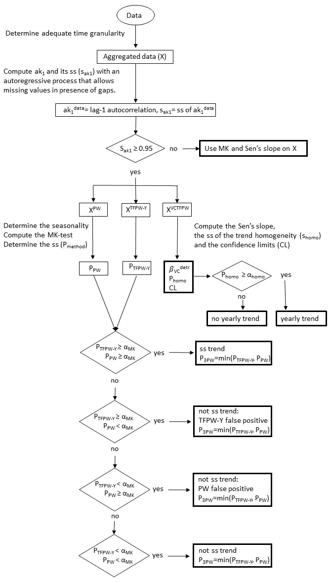
Figure 1 Scheme of the new 3PW algorithm. α_MK is the desired confidence limit for the MK test and α_homo the desired confidence limit for the homogeneity test between temporal segments. The values applied for this study are α_MK=0.95 and α_homo=0.90.

3 Experimental

In order to have a broader view of the effects of the various PW methods, several very different time series (Table 2) were used: three surface in situ aerosol properties (absorption coefficient, scattering coefficient and number concentration) measured at Bondville (BND), a remote, rural station in Illinois, USA; the aerosol optical depth (AOD) measured at Payerne (PAY) on the Swiss plateau; the tropopause and the zero-degree temperature levels measured by radio-sounding launched at PAY; and the water vapor mixing ratio at 1015 m measured by remote sensing at PAY. The shortest time series (AOD and water vapor mixing ratio) cover only 10 years of measurements, while the longest time series cover 60 years. The three in situ aerosol properties are Johnson-distributed and diverge strongly from a normal distribution. The other time series exhibit distributions that also diverge from a normal distribution but to a lower extent, such that some of them have residuals of a least mean square fit, which are normally distributed. The values of some of the time series span over several orders of magnitude and the scattering and absorption coefficients time series contains negative values due to detection limit issues in very clean conditions. The time series of the zero-degree temperature level also includes negative altitudes, since it is interpolated to altitudes lower than sea level in the case of negative ground temperature at PAY (Bader et al., 2019). All the data have high ${\text{ak}}_{\mathrm{1}}^{\mathrm{data}}$ at the daily time granularity and exhibit clear seasonal cycles with maxima in summer.

Table 2 Description of the time series: time series with units, monitoring station, period, instrument type, original granularity, ranges (1 and 99 percentiles (1%ile and 99%ile)), mean, median and standard deviation (SD), lag-1 autocorrelation of the observations (${\text{ak}}_{\mathrm{1}}^{\mathrm{data}}$) and number of ss partial autocorrelations for the 10-year period (order), number of daily data in the 10-year period (N) and reference.

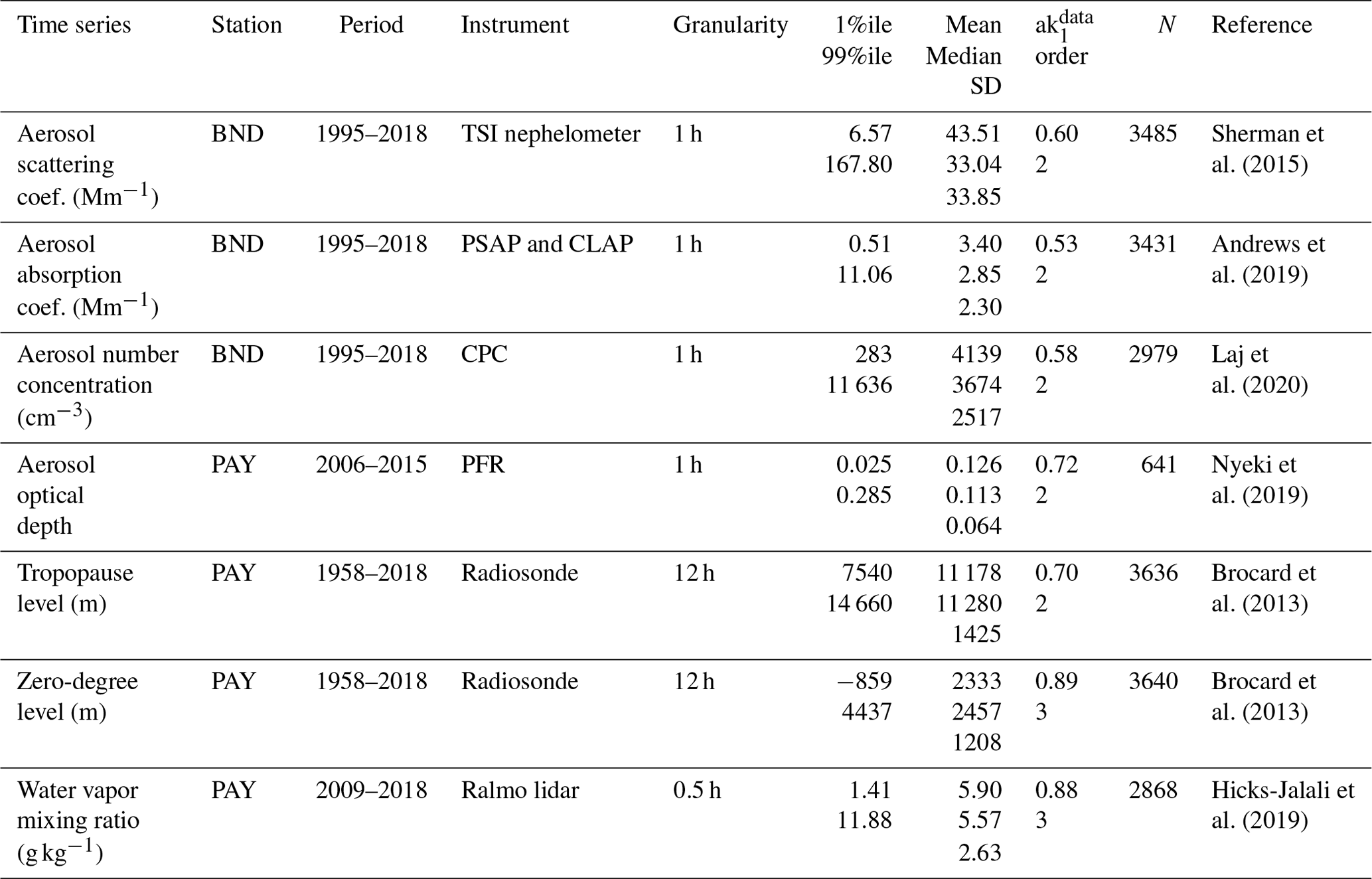
PSAP: particle soot absorption photometer; CLAP: continuous light absorption photometer; CPC: condensation particle counter, PFR: precision filter radiometer.

Trend analyses were applied to several periods. For all the data sets, the last 10-year period (e.g., 2009–2018 for the BND aerosol scattering coefficient) is considered first and then further possible multi-decadal periods (e.g. the last 20 years, 1999–2018; 30 years, 1989–2018) up to 60 years for the radio-sounding time series. For the in situ aerosol properties, tests with 4- to 9-year periods are also computed in order to illustrate the problems of trend analysis on very short time series. The number of data points in the time series (N) depends on the length of the period and on the time granularity. The choice of temporal segmentation to address seasonality for the seasonal MK tests can also affect N and was evaluated by segmenting the time series into months and meteorological seasons (December–February, March–May, June–August, September–December) for time granularities up to 1 month. The MK test was also applied to the complete time series without considering seasonality (no temporal segmentation) for comparison purposes, even though, properly, seasonal MK tests must be used when seasonal cycles are present.

To assess the statistical significance, the two-tailed p values are computed. For a more comprehensive presentation of the results, the statistical significance is presented here as 1 minus p value so that the ss at a 95 % confidence level is effectively given by ss=0.95. If not further specified, the ss of the trend and of ${\text{ak}}_{\mathrm{1}}^{\mathrm{data}}$ is given at the 95 % confidence level, whereas CLs and X_homo are given at the 90 % confidence level. The slopes (in percent) are normalized by the median of the data. Periods of at least 10 years and trends on these periods are further called decadal periods and decadal trends.

4 Results and discussion

As explained in the methodology section (Sect. 2), the trend results (e.g., the ss, the slopes and the CLs) depend on a number of factors, the most important ones being the prewhitening method, the number of data points in the time series and the presence of autocorrelation. The choice of the prewhitening method clearly affects the ss, the slope and the CLs. Analysis choices such as the time granularity, the length of the analyzed period and the temporal segmentation to address seasonality affect ${\text{ak}}_{\mathrm{1}}^{\mathrm{data}}$, N and the variance of the time series. There is a pronounced interdependency among these variables involving critical choices in the presentation of the results. Some general plots are first presented to provide insights into the primary results for some of the time series. They are followed by a more detailed analysis of the effects of the prewhitening method, the time granularity, the temporal segmentation, the length of the data series and the number of data points in the time series.

MK trend results (Fig. 2) of the aerosol number concentration, the aerosol scattering coefficient, the tropopause level and the AOD are plotted as a function of the time granularity for the MK test and for all the prewhitening methods. The discrepancy between the results computed with no temporal segmentation and for two different temporal segmentations to address seasonality (four meteorological seasons and 12 months) can be estimated from the inserted boxplots. The three aerosol properties exhibit decreasing trends, while the results of the tropopause level time series indicate a positive trend. The negative aerosol slopes are related to the decreasing aerosol load in western Europe and North America (Collaud Coen et al., 2020; Yoon et al., 2016). The increasing tropopause level trend is related to global warming (Xian and Homeyer, 2019). The results of the trends will not be further described and discussed, since this study is only focused on the methodology of the trend analysis.

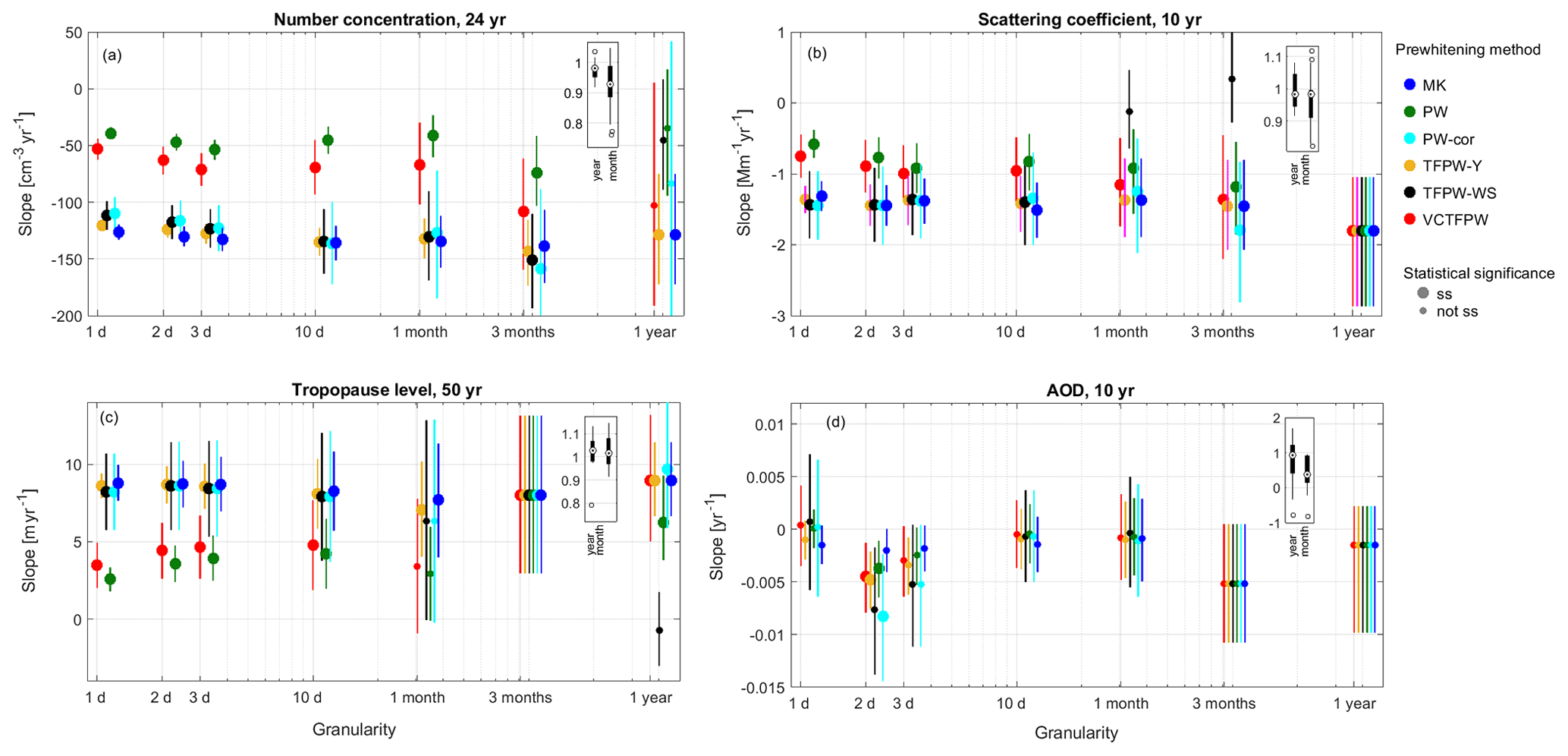
Figure 2 Slope and confidence limits computed without temporal segmentation as a function of the time granularity for MK and the five prewhitening methods (indicated by colors) for (a) the aerosol number concentration for the 24-year period, (b) the aerosol scattering coefficient for the 10-year period, (c) the tropopause level altitude for the 50-year period, and (d) the AOD for the 10-year period. Larger symbols indicate ss trends. Inserted boxplots indicate the median, the quartiles and the whiskers of the ratio between the slopes computed with no temporal segmentation (year) and with the temporal segmentation of 12 months (month) over the slopes computed with the temporal segmentation of four meteorological seasons.

The common features for all the time series considered here are the following.

• -

  The MK, TFPW-Y, TFPW-WS and PW-cor methods result in similar slopes.

• -

  As described in Wang et al. (2015a), the absolute value of the VCTFPW slopes lies between the TFPW and the PW slope values. The absolute value of the PW slopes is always smaller than the TFPW slope values.

• -

  Large time aggregations usually lead to not ss ${\text{ak}}_{\mathrm{1}}^{\mathrm{data}}$ and, consequently, prewhitening methods do not need to be applied to those cases. The ${\text{ak}}_{\mathrm{1}}^{\mathrm{data}}$ of all prewhitening methods is not ss for 3-month aggregations of the tropopause level and AOD data sets and for 1-year aggregation of the aerosol scattering coefficient and AOD. The ${\text{ak}}_{\mathrm{1}}^{\mathrm{data}}$ of the aerosol number concentration remains ss until the 1-year aggregation.

• -

  CLs are smaller for finer time granularities in the presence of ss ${\text{ak}}_{\mathrm{1}}^{\mathrm{data}}$.

• -

  CLs of MK, PW and TFPW-Y, which remove the lag-1 autocorrelation without compensation for the mean values and the variances of the original time series, are smaller than for VCTFPW, PW-cor and TFPW-WS. PW-cor and TFPW-WS have the highest CLs.

• -

  The ss often decreases for coarser time granularities, occasionally leading to not ss trends for some of the prewhitening methods. PW, TFPW-WS and VCTFPW methods become not ss at finer time granularities than TFPW-Y and MK due to their lower number of false positives.

• -

  The slope discrepancies between prewhitening methods are larger than the discrepancies that occur when different temporal segmentations (months or meteorological seasons) are applied for a defined prewhitening method.

Apart from these general observations, there are features that depend on the time series, such as the effects of the applied temporal segmentation to address seasonality, the similarity of MK slopes to TFPW slopes, and the time granularity leading to not ss ${\text{ak}}_{\mathrm{1}}^{\mathrm{data}}$. For example, the very low number of data points in the AOD time series (about 65 per year) corresponds to an average of 1 datum per 5 d; there is consequently a very high number of missing values for time granularities finer than this measurement frequency, and this induces higher CLs for time granularities of 1–3 d than granularity of 10 d.

4.1 Effects of the prewhitening methods

As predicted theoretically, the ss depends on the prewhitening method, with higher ss for the MK and TFPW-Y methods that are related to higher type 1 errors (false positives), while PW and VCTFPW have a lower ss and a lower test power. This is verified on the individual time series, e.g., for the aerosol number concentration results presented in Fig. 3a. The yearly trend was computed for all periods (from 5 to 24 years) at all considered time granularities (1 d to 1 month for the meteorological season temporal segmentation), leading to 40 trends. The results show the following.

• -

  The MK test ss without prewhitening has a median of 1, with the ss for the upper quartile and upper whisker also equal to 1 and thus within the 95 % confidence level, so that only 5 trends out of 40 evaluated (i.e., 12.5 %) are not ss.

• -

  The TFPW-Y ss has a median slightly lower than 1 and only three trends (7.5 %) outside the 95 % confidence level.

• -

  The TFPW-WS ss has a median of 0.996, which is lower than MK and TFPW-Y. The lower quartile for TFPW-WS is 0.89, which is outside the 95 % confidence level and indicates that 32.5 % of the trends are not ss.

• -

  The results of both PW and PW-cor are similar to the TFPW-WS, with a median ss of 0.995, a lower quartile of 0.84 %, and 32.5 % of the trends are not ss.

• -

  The VCTFPW ss has the lowest median (0.98), first quartile (0.83) and lower whisker (0.63), leading to 37.5 % of trends being not ss.

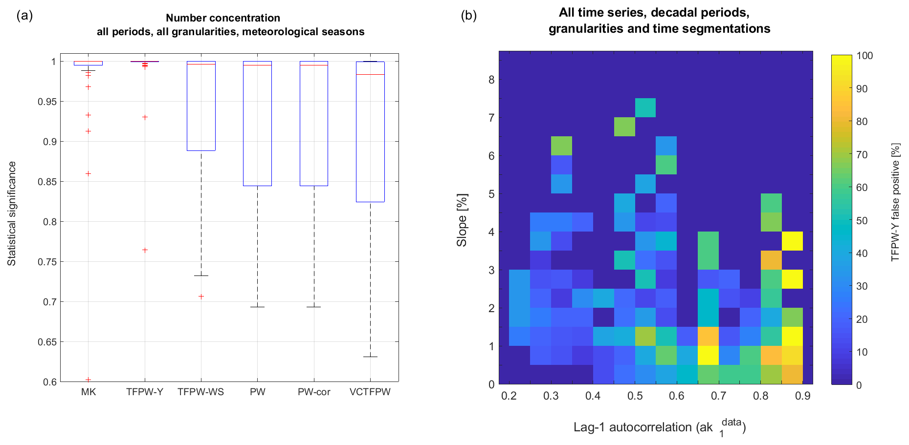
Figure 3 (a) Statistical significance of trends as a function of the prewhitening methods for the aerosol number concentration for the yearly trends computed from four meteorological seasons' time segmentation, for all periods (5 to 24 years) and all time granularities (1 d to 1 month). This represents 40 trends. The median is represented by the red line, the boxes are the 25 % and 75 % percentiles, the whiskers the 0.7 and 99.3 percentiles and the red plus signs the outliers. Some outliers are not in the figure for purposes of clarity. (b) Number of TFPW-Y false positives as a function of ${\text{ak}}_{\mathrm{1}}^{\mathrm{data}}$ and slope categories for all the computed trends of all time series for all decadal periods. Categories with fewer than three points are not plotted.

Similar results are found for all time series but with less difference amongst the methods when the trends are obviously present or absent and more differences for weak trends.

According to Monte Carlo simulations presented in the literature (e.g., Yue et al., 2002; Wang et al., 2015a; Hardison et al., 2019), TFPW-Y leads to a high number of false positives. Since this study deals with measured data, the rate of false positives is defined as trends that are ss with TFPW-Y but not ss with PW, since the latter is the method with the lowest rate of type 1 error. Figure 3b shows that the number of false positives depends, as expected, on the strength of the slope and on ${\text{ak}}_{\mathrm{1}}^{\mathrm{data}}$. Weaker trends (smaller slopes in percent) are usually associated with lower ss and consequently lead to a larger number of false positives. The impact of the PW and TFPW-Y depends largely on ${\text{ak}}_{\mathrm{1}}^{\mathrm{data}}$ absolute values; i.e., higher ${\text{ak}}_{\mathrm{1}}^{\mathrm{data}}$ leads to stronger modification of the original time series with lower means (e.g., the mean of $X_t^{\mathrm{PW}}$ is less than the mean of X_t) and reduced variances for positive ${\text{ak}}_{\mathrm{1}}^{\mathrm{data}}$. The highest ${\text{ak}}_{\mathrm{1}}^{\mathrm{data}}$ values (between 0.85 and 0.9) found in the time series studied lead to 60 % to 100 % false positives, while ${\text{ak}}_{\mathrm{1}}^{\mathrm{data}}$ values between 0.8 and 0.85 lead to at least 40 % false positives.

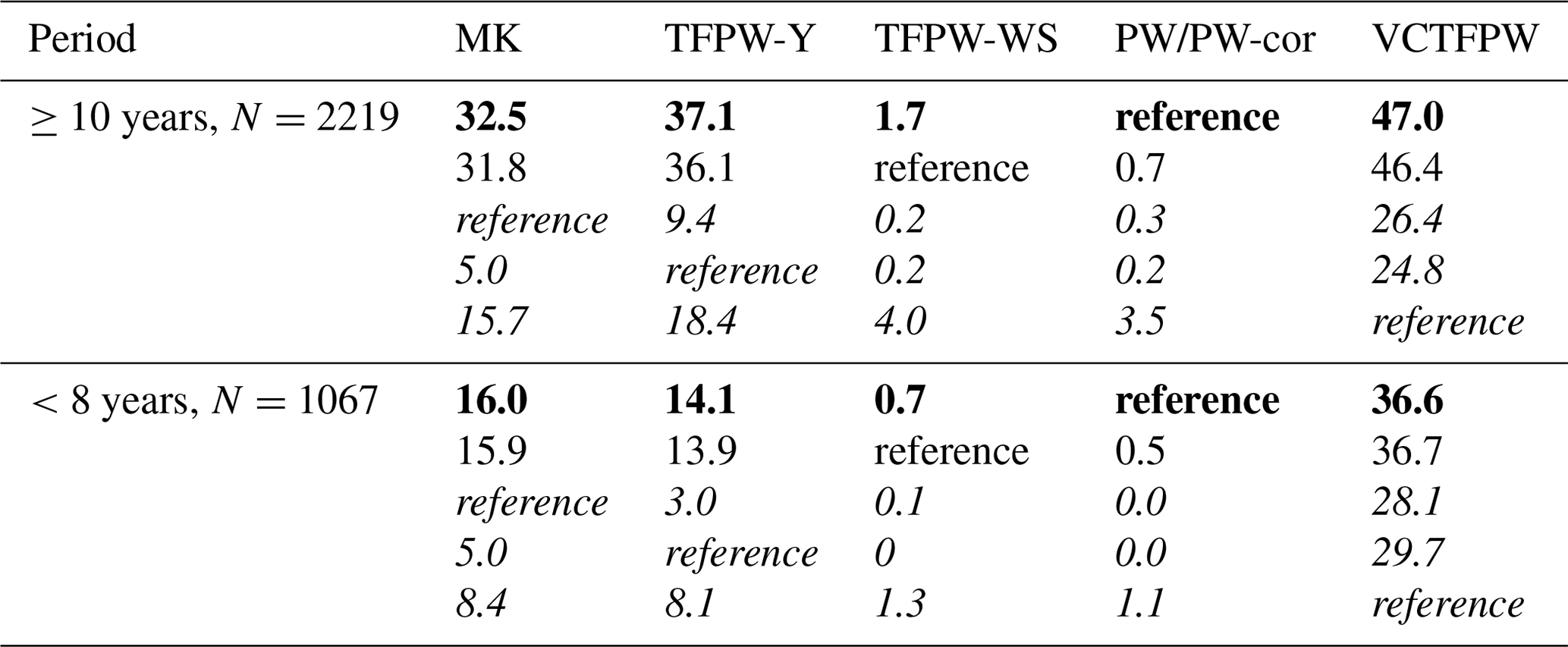
To obtain a better view of the weakness of each MK test, the percentage of false positives taking each of the prewhitening methods as a reference is reported in Table 3 for all the data sets. PW-cor has by definition the same ss as PW, so that their performances are given in the same column. PW has to be used as the best reference for false positives because it is the prewhitening method with the lowest sensitivity to type 1 errors (Zhang and Zwiers, 2004; Yue et al., 2002; Blain, 2013; Wang et al., 2015a), whereas the consideration of the other prewhitening methods as references allows for the evaluation of the discrepancy in ss among the methods. For the decadal trends, MK, TFPW-Y and VCTFPW have 32 %–47 % of false positives taking PW as a reference. This suggests that about two-thirds and half of the trends determined using TFPW-Y and VCTFPW, respectively, are false positives. TFPW-WS has less than 2 % of false positives, so that it can be considered to have equivalent performance to PW. For the trends on short periods, the lower amounts of false positive for MK and TFPW-Y are due to the overestimation of the slopes with these tests (see Sect. 4.4), leading to trends that are more robust and enhanced ss. The unbiased estimate of the VCTFPW slope produces similar amounts of errors for the short-term trends to those for the decadal trends. The percentage of false positives is similar if TFPW-WS is considered the reference. If MK or TFPW-Y is taken as a reference, PW and TFPW-WS have a very low number of false positives independent of the length of the period, leading to the conclusion that few cases remain uncertain. Note that 5 %–10 % of cases have different ss at the 95 % confidence level if MK or TFPW-Y is used as a reference, indicating that estimation of the ss using these two methods can have a slight impact on the results. Finally, all the prewhitening methods have a higher number of false positives if VCTFPW is considered the reference because the added slope at the end of the VCTFPW procedure is smaller than the initial slope and leads to less detectable trends. Note also that the percentage of false positives of PW and TFPW-WS remains low (≤4 %) for all the chosen references. For the time series considered in this study, the following conclusions can be made: (1) PW (and PW-cor) performs very well with a small (≤3.5 %) number of false positives if other prewhitening methods are considered the reference; (2) TFPW-WS has a very low number of false positives (<2 % if PW is taken as the reference); (3) VCTFPW exhibits a high rate of type 1 errors and should consequently not be used to determine the ss; and (4) the difference in ss between MK and TFPW-Y is related to only 5 %–10 % of the trends.

Table 3 Percent of false positives for all data sets relative to a reference test for the MK tests and prewhitening methods for periods of at least 10 years (decadal trends) or smaller than 8 years. N is the number of considered trends. PW should be considered the best reference so that the results are given in bold. MK, TFPW-Y and VCTFPW have a higher number of type 1 errors and should not be considered a reference so that these results are given in italic.

The effects of the prewhitening method on the slope (Figs. 2 and 4) also follow the theoretically deduced assumptions.

• -

  The slope estimated on the original data is always enhanced by the positive ${\text{ak}}_{\mathrm{1}}^{\mathrm{data}}$, which adds a multiple of the t−1 value to the t value (e.g., Eqs. 1 and 3). By removing the autocorrelation, PW leads to a strong decrease in the absolute value of the slope that becomes smaller than the MK slope. The CL_PW are also somewhat decreased (Fig. 5) due to the decreased mean and variance of the prewhitened time series, relative to the original data set.

• -

  Due to the detrending procedure, the absolute values of the TFPW-Y slope are larger than the PW slopes and similar to the MK slope values (Fig. 2), even if a tendency to have larger TFPW-Y than MK slopes is observed (Fig. 4b). The CL_TFPW−Y are similar to the CL_PW because the variance and mean are similar for both the PW and TFPW-Y prewhitened time series.

• -

  Due to the corrected slope and variance, the absolute values of the VCTFPW slopes are much smaller than the TFPW-Y slopes but larger than the PW slopes.

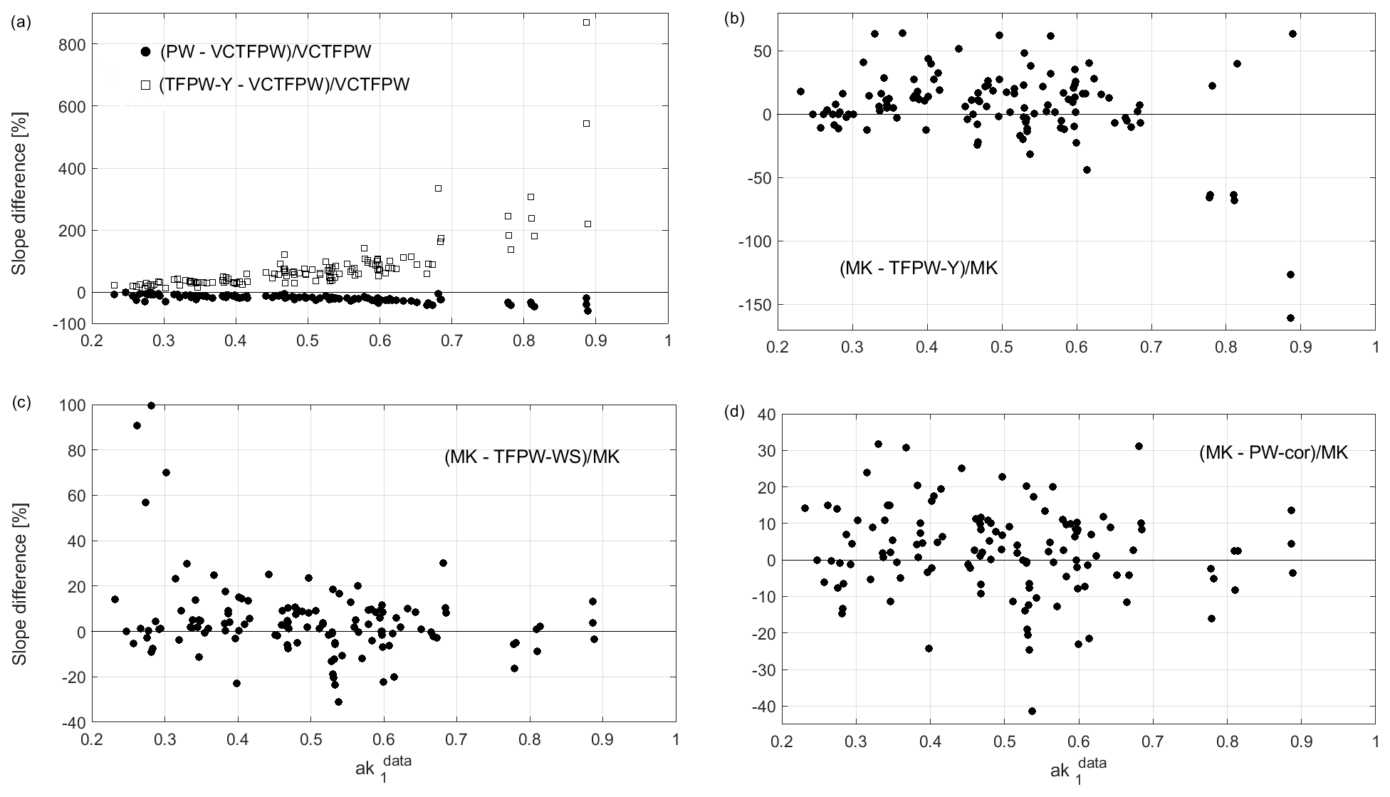
Figure 4 Slope differences as a function of ${\text{ak}}_{\mathrm{1}}^{\mathrm{data}}$ from the original data for all data sets, granularities and periods and for meteorological season time segmentation: (a) PW minus VCTFPW slope (filled dots) and TFPW-Y minus VCTFPW slope (open squares) normalized by the VCTFPW slope, (b) MK slope minus TFPW-Y slopes, (c) MK minus TFPW-WS slopes and (d) MK minus PW-cor slopes. The slope differences in (b, c, d) are normalized by MK slope. Not ss trends (PW taken as reference) are not plotted since the slopes cannot be distinguished from the zero trend. Note the different y axis ranges in these plots.

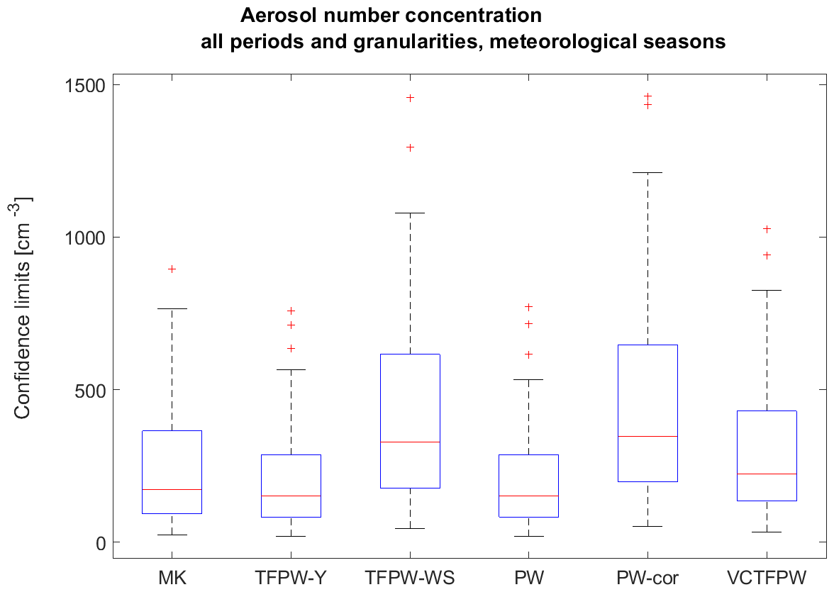
Figure 5 Distribution of the confidence limit intervals of the slope for the trend in aerosol number concentration for all periods (5–24 years) and time granularities (1 d–1 month) as a function of the method for the meteorological season temporal segmentation. Box–whisker plotting as described for Fig. 3a.

These theoretical assumptions are validated in all cases with the ss trends analyzed in this study. The water vapor mixing ratio and the zero-degree level both have a very high autocorrelation (about 0.9 at 1 d time granularity). In such cases, the removal of the autocorrelation can lead to

Not ss trends and the absolute values of the VCTFPW slope are not always larger than PW slope values.

The slope difference among the methods depends directly on ${\text{ak}}_{\mathrm{1}}^{\mathrm{data}}$. A more nuanced estimate of the slope dependence is shown in Fig. 4, where the differences among the prewhitening methods are plotted. As already mentioned, the VCTFPW method largely mitigates the slope overestimate of the TFPW-Y method at large ${\text{ak}}_{\mathrm{1}}^{\mathrm{data}}$ so that the increase in the slope absolute value for increasing ${\text{ak}}_{\mathrm{1}}^{\mathrm{data}}$ does not exceed a factor of 2 (100 % difference in Fig. 4a). The difference between VCTFPW and TFPW-Y slopes can reach 200 %–1000 % for the largest ${\text{ak}}_{\mathrm{1}}^{\mathrm{data}}$. The overestimation of the slope by TFPW-Y is much larger than the underestimation by PW if VCTFPW is taken as a reference for slope estimation. TFPW-Y slopes tend to be larger than MK slopes (Fig. 4b), with larger differences at high ${\text{ak}}_{\mathrm{1}}^{\mathrm{data}}$. Finally, the slope difference between MK and both TFPW-WS and PW-cor does not depend on ${\text{ak}}_{\mathrm{1}}^{\mathrm{data}}$, and the TFPW-WS and PW-cor slopes are usually nearly identical, as suggested by their similar relationship to the MK slope (Fig. 4c, d).

The effects of the prewhitening method on CLs (Fig. 5) are explained by their modification of the mean and the variance of the data. Removing the lag-1 autocorrelation leads to prewhitened data with a larger variance but lower mean than the original time series. The correcting factor of $(\mathrm{1}-{\text{ak}}_{\mathrm{1}}{)}^{-\mathrm{1}}$ used in the TFPW-WS and PW-cor methods restores the mean (Eq. 5), whereas the VCPWTF method restores the initial variance (Eq. 9). All increases in the variance make the CL interval wider, whereas the decrease in the mean decreases the CL interval. CL_TFPW−Y and CL_PW are the narrowest due to lower mean and variance values, while CL_TFPW−WS and CL_PW−cor are the widest due to larger variance induced by the prewhitening and a mean identical to the original data. CL_VCTFPW are intermediate with a variance similar to the original data but a lower mean.

4.2 Effects of the time granularity

Averaging is often used to decrease ${\text{ak}}_{\mathrm{1}}^{\mathrm{data}}$ in the time series. To investigate this, the ${\text{ak}}_{\mathrm{1}}^{\mathrm{data}}$ values are plotted as a function of the time granularity for the last 10 years of all the time series (Fig. 6a). The decrease in ${\text{ak}}_{\mathrm{1}}^{\mathrm{data}}$ with aggregation does not have a large impact until granularity is coarser than 1 month. For 1-month time granularity and less, aggregation leads to an ${\text{ak}}_{\mathrm{1}}^{\mathrm{data}}$ difference smaller than 0.2 in five of the time series. Three-month and 1-year aggregations involve a sharper reduction of ${\text{ak}}_{\mathrm{1}}^{\mathrm{data}}$. Additionally ${\text{ak}}_{\mathrm{1}}^{\mathrm{data}}$ for 1-year aggregation is, for most of the time series, no longer ss and, sometimes, even negative. The decrease in ${\text{ak}}_{\mathrm{1}}^{\mathrm{data}}$ is not continuous with time granularity, with ${\text{ak}}_{\mathrm{1}}^{\mathrm{data}}$ often larger for 10 d or 1 month than for 3 d aggregation. These local minima can be explained by a competitive effect between the ${\text{ak}}_{\mathrm{1}}^{\mathrm{data}}$ decrease and a reduction of the measurement variance. For the 10-year period represented in Fig. 6, none of the ${\text{ak}}_{\mathrm{1}}^{\mathrm{data}}$ values are ss for a 1-year time granularity. However, there are cases like the 24-year time series of the aerosol number concentration where ${\text{ak}}_{\mathrm{1}}^{\mathrm{data}}$ is still ss for the 1-year time granularity. In these cases, prewhitening methods have to be applied, which leads to the spread of the slopes for the various prewhitening methods visible in Fig. 2a.

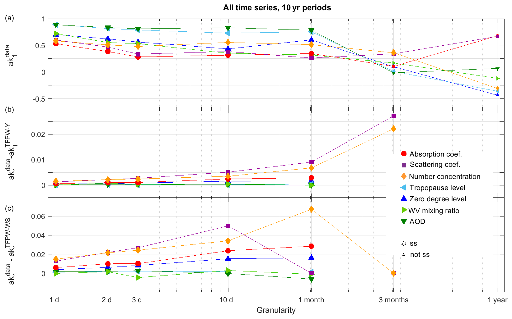
Figure 6 (a) Lag-1 autocorrelation (${\text{ak}}_{\mathrm{1}}^{\mathrm{data}}$) of the original data as a function of the time granularity for the 10-year time series of all parameters; bigger symbols correspond to ss ${\text{ak}}_{\mathrm{1}}^{\mathrm{data}}$, (b) ak₁ difference between the original data and the TFPW-Y data, and (c) ak₁ difference between the original data and the TFPW-WS data. For (b, c) only ss cases are plotted because prewhitening methods are not applied when ak₁ is not ss.

TFPW-Y and TFPW-WS remove the autocorrelation computed from the detrended data. Figure 6b and c show the difference in ak₁ between the original and the detrended time series as a function of the time granularity. The ${\text{ak}}_{\mathrm{1}}^{\mathrm{detr}}$ continuously increases with aggregation, whereas ${\text{ak}}_{\mathrm{1}}^{detr-prew,n}$ sometimes decreases (e.g., for 1- or 3-month aggregations for scattering coefficient and number concentration, respectively). While the differences in ak₁ from the original time series are larger for TFPW-WS than for TFPW-Y, they remain relatively small and exceed 0.05 only in a few cases.

Figure 7 presents the effect of the time granularity on ss of the trends for the zero-degree temperature level for different periods (identified by colors) and various prewhitening methods (identified by symbols). MK and PW-cor are not included since their ss values are nearly identical to the TFPW-Y and PW ss values, respectively. As expected, TFPW-Y exhibits the highest ss, followed by TFPW-WS, while PW and VCTFPW exhibit the lowest ss. The ss always decreases at coarser time granularities for all prewhitening methods until ${\text{ak}}_{\mathrm{1}}^{\mathrm{data}}$ becomes not ss, usually at an average of 3 months. This decrease in ss is larger for the PW, TFPW-WS and VCTFPW than for TFPW-Y. For robust trends analyzed (e.g., the period of 40 years in Fig. 7), the trend is ss at the 95 % or 90 % confidence level for the finest time granularity (3 d for PW and TFPW-WS and 1 month for TFPW-Y ), but this is often not the case for weak trends.

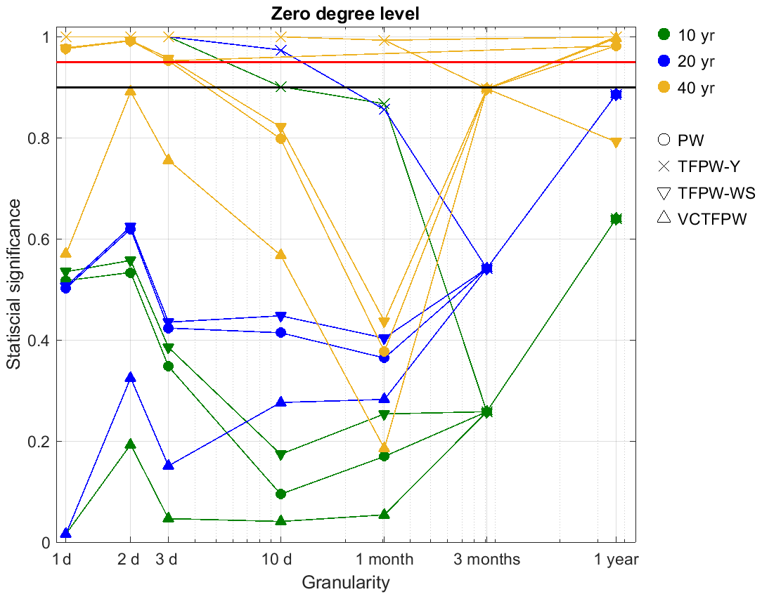
Figure 7 Statistical significance of the trends as a function of the time granularity and prewhitening methods for the zero-degree level time series for 10-, 20- and 40-year periods without temporal segmentation to address seasonality. The horizontal red and black lines correspond to the threshold of 95 % and 90 % confidence levels, respectively.

When ${\text{ak}}_{\mathrm{1}}^{\mathrm{data}}$ is not ss at high time granularity, the prewhitening methods can no longer be applied and the ss is similar for all methods. Without prewhitening, the ss is inversely proportional to the variance reduction caused by the aggregation. For TFPW-Y, the removal of the prewhitening due to not ss ${\text{ak}}_{\mathrm{1}}^{\mathrm{data}}$ at 3-month aggregation corresponds however to a decrease in the ss of the trend. The ${\text{ak}}_{\mathrm{1}}^{\mathrm{detr}-\mathrm{prew},n}$ of the 40-year period is ss for the 1-year time granularity, as can be seen by the TFPW-WS ss that is different than the ss of the other prewhitening methods (Fig. 7), leading to lower ss than without prewhitening. The increase in the ss with the period length is also obvious, with smaller differences between TFPW-Y and PW for longer periods. The longest period (40 years) and the finest time granularities (1–3 d) lead to no false positives for TFPW-Y, which is not the case for shorter periods or coarser time granularities.

The effect of the time granularity on the slope strongly correlates with the ak₁ time granularity dependence. A decrease in the autocorrelation with aggregation induces a reduction of the prewhitening effects on the slopes, leading to a decrease in the differences between slopes (see Figs. 2 and 4).

The loss of ss with coarser time granularities is even more pronounced when evaluated for each month or meteorological season (Fig. 8). This is due to the lower N per season (1∕4 for meteorological season and 1∕12 for months). Similarly, the decrease in the difference in slopes due to aggregation and the reduction of the prewhitening effects are both more pronounced when temporal segmentation is applied due to the reduction of the number of data points in each temporal segment.

Figure 8 VCTFPW slope (dots) and CL (vertical lines) as a function of the time granularity for the division of the time series into (a) 12 months for the 10-year aerosol scattering coefficient and (b) into four meteorological seasons for the 10-year aerosol absorption coefficient. Larger symbols indicate statistically significant slopes computed from 3PW.

Figure 8 clearly shows that the coarsest time granularities enhance the variability for the different temporal segmentation choices. For example, the interval between the minimum and maximum slopes is 2.3 times larger for the monthly average than for the daily average for the scattering coefficient temporally segmented into 12 months (Fig. 8a) and 3.7 times larger for the absorption coefficient with meteorological seasons (Fig. 8b), respectively. In some cases, the sign of the slope changes with the time granularity when the trends are not ss. As already observed in Fig. 2, the CLs also increase with time granularity due to the decrease in N. The effects of the time granularity on the ss, the slope and the CLs are more pronounced for a monthly than for meteorological season temporal segmentation due to N being 3 times lower for the months than it is for the seasons.

4.3 Effects of temporal segmentation to address seasonality

The division of the year into temporal segments is a necessary condition of the MK test if the data exhibit a clear seasonality. Statistically, it is important to have equivalent segments with similar lengths to obtain similar N per segment. The time series presented in this study are all dependent on phenomena related to the temperature (e.g., atmospheric circulation, boundary layer height, source changes) and thus change with the meteorological seasons. The seasonality of time series primarily affected by other meteorological phenomena (e.g., the Asian monsoon, which is better characterized by dry and humid seasons, rather than the standard four meteorological seasons) has to be carefully studied in order to choose both the appropriate temporal segmentation and the appropriate time granularity. For example, a time granularity that does not respect the seasonal variation of a time series can lead to erratic results (de Jong and de Bruin, 2012).

The effects of the chosen temporal segmentation to address seasonality are presented here for the VCTFPW slope and CLs, but they are similar for the other methods as well. The effect of including temporal segmentation on the ss of the yearly trend is rather small, with a difference of only 2 %–3 % in the number of ss trends (not shown). The division into four meteorological seasons always results in the largest number of ss trends, while the division into 12 months is less powerful for short periods due to the low number of points for each month (N≤10) for a 10-year period. The application of no temporal segmentation, which does not meet the MK-test requirements in the presence of a seasonality, is less powerful for decadal trends. No systematic effects due to the choice of temporal segmentation on the slope were found. Different temporal segmentation choices lead, most of the time, to comparable slopes. The effect of the prewhitening method is always much more pronounced than the effect of the choice of temporal segmentation.

Figure 9 presents the CL intervals normalized by the trend slope as a function of the time granularity for the aerosol scattering coefficient without temporal segmentation (blue) or divided into monthly (green) or meteorological seasons (red) for several periods between 5 and 24 years. Due to the decrease in N, finer temporal segments induce an increase in the CLs. In the case presented in Fig. 9, monthly segments have CL intervals 4 times larger than when seasonality is not considered and 2 times larger than meteorological seasons for the longest periods. It should be recalled, however, that not considering seasonality for time granularity finer than 1 year is not allowed due to the observed seasonal variation in the aerosol scattering coefficient time series.

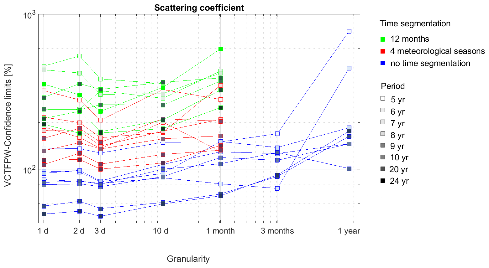
Figure 9 Confidence limits of VCTFPW as a function of the time granularity for various periods of the aerosol scattering coefficient time series. Blue represents no consideration of seasonalities; red represents time segmentation into four meteorological seasons and green into 12 months. The color shading corresponds to the length of the period from 5 years (lightest) to 24 years (darkest).

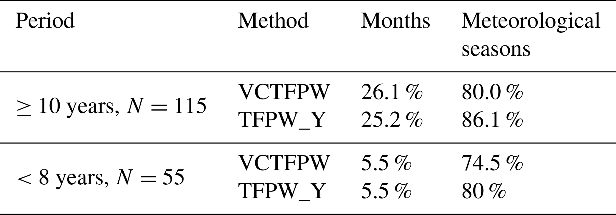
In the case of a seasonal MK test, yearly trend results can be considered only if the trends are homogeneous among the temporal segments (see Sect. 2.1). The division of the time series into four meteorological seasons leads to more homogeneous trends (3 times and 25 times for decadal and short periods, respectively) at the 90 % confidence level than the division into 12 months (Table 4). Thus, if meteorological seasons correspond to the observed temporal cycle of the studied time series, then those seasons should be the preferred temporal division to consider rather than monthly divisions. Monthly segmentation could be considered when the observed variability of time series is shorter or longer than the 3-month length of a meteorological season.

Table 4 Percentage of yearly trends with homogeneous temporal segments as a function of the type of segment (month or season), of the prewhitening method and of the length of the periods based on all seven time series considered in this study.

4.4 Effects of length of the time series

As already stipulated under Sect. 2.1, a special statistic that deviates from the normal statistic has to be applied to compute the statistical significance for N≤10. Shorter periods involve smaller N, and N is further affected by the choice of granularity. The special statistic has to be applied for trends computed on 1-year averages and periods <11 years (i.e., N≤10). Note: the effect of the natural variability of a data set on trends computed on short periods will not be directly discussed here, but only the statistical effect on the trends determined for the various time series studied here.

Figure 10 shows the effect of the reduction of the period length on the slope, the CL and the ss for the aerosol absorption coefficient data set. The first obvious effect is that the absolute values of the slope are larger for shorter periods and that there are large differences for both the individual months and meteorological seasons. Further, these large slopes for short time periods are associated with high CLs and low ss. They are due to the cumulative effects of the predominant importance of the first and last years for short periods and to the low N in the time series. For the shortest period considered here (4 years), the division of a daily time series into four meteorological seasons involves trends computed with N=360 (=4 years ×3 months ×30 d), whereas monthly trends for the same time series are computed with N=120 (=4 years ×1 month ×30 d). The reduction of N by a factor of 3 explains the larger and more variable slope values, the higher CLs and the lower ss of the monthly trends compared to the meteorological season's trends. The effects due to the reduction of N are minimized by the use of daily time granularity, but they are maximized by the use of larger aggregations leading for example to N=12 and 4, respectively, for monthly aggregation (hence the tendency for increases in CLs with larger aggregation in Fig. 9). It should be noted that the influence of the length of the time series is usually more important than the choice of time granularity. For short time series, the yearly slopes can differ depending on the chosen temporal segmentation (see, e.g., the yearly slopes of 5, 6 and 7 years in Fig. 10). These results, then, support the standard recommendation of only computing long-term trends on time series of at least 10 years.

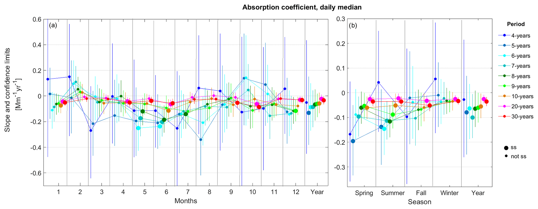
Figure 10 VCTFPW slopes (dots) and CLs (vertical lines) as a function of various periods ending in 2018 for the daily aerosol absorption coefficient for the division of the time series into (a) 12 months and (b) four meteorological seasons. Colors represent time period lengths and bigger symbols represent ss trends with the 3PW method.

4.5 Effects of the number of data points

The number of data points N in the time series is a key variable underlying the effects of the time granularity, the temporal segmentation to address seasonality and the period discussed in the previous sections. Because a long-term trend analysis is statistically sound only for time series of at least a decade in length, only decadal and multi-decadal trends are considered in this section. Figure 11 is computed using 3PW (e.g., Fig. 1) for all decadal trends for all time series, temporal segmentation choices and time granularities and represents the percentage of ss trend as a function of slope and N categories. Figure 11a shows that time series with robust trends, identified by high normalized slopes, need fewer data points to reach the 95 % confidence level significance than time series with less robust trends. In contrast, weaker trends, identified by low normalized slopes, need at least several hundreds or even thousands of data points to become ss. In consequence, the smallest slopes need longer periods and finer time granularities to be identified as statistically significant.

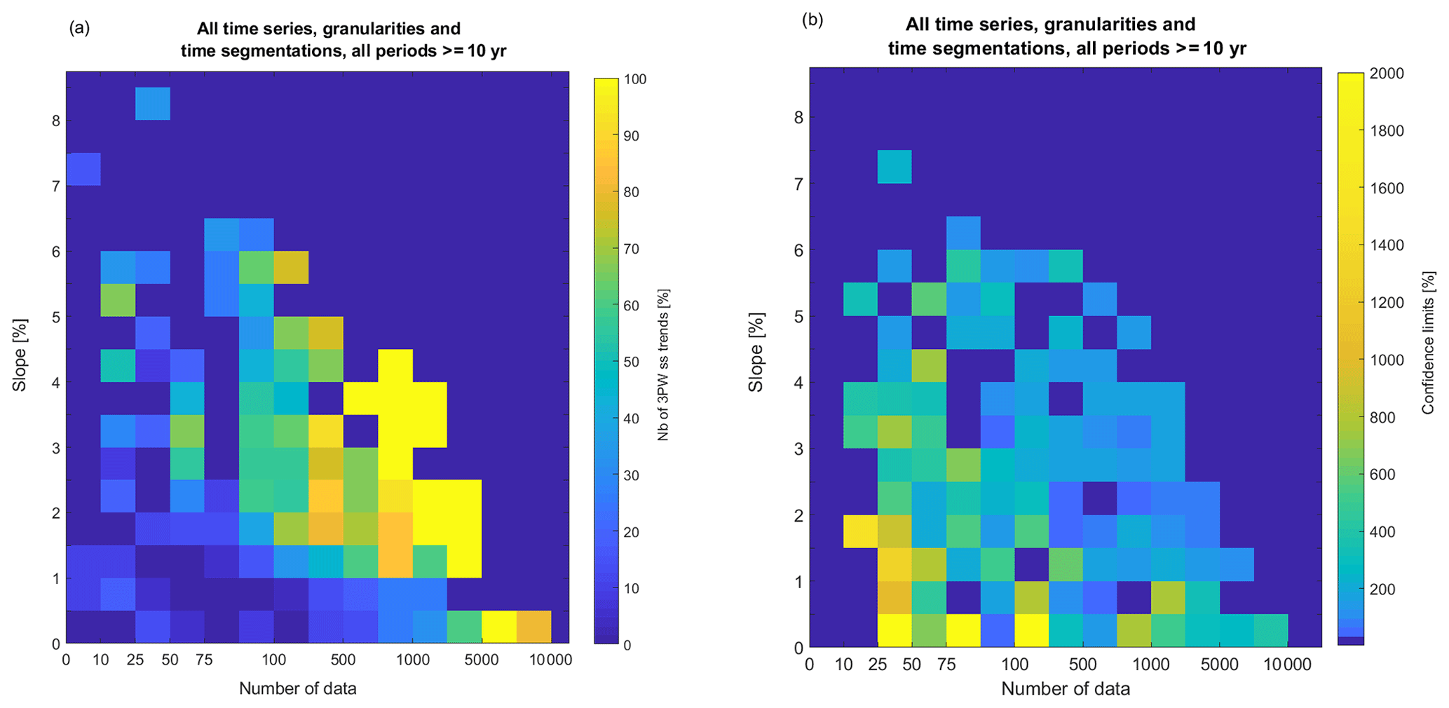
Figure 11 (a) The percentage of 3PW ss trends (Sect. 2.3) and (b) mean confidence limits normalized by the slope as a function of slope normalized by the median and N categories for all time series, granularities and time segmentations and all periods of at least a decade. The slopes are binned regularly (bin size =0.5 %), but N categories are irregular. Cells with fewer than three results were discarded in panel (a).

Figure 11 also clearly shows that small N leads statistically to larger normalized slopes and thus demonstrates that trends computed on short periods and with a long averaging time are usually greatly overestimated. The use of prewhitening methods with a large type 1 error will, in addition, falsely indicate ss trends (see Sect. 4.1 and Table 3). The use of MK or TFPW-Y tests on short, highly autocorrelated, and highly aggregated time series will definitely produce false positive trends with high absolute slopes.

The effects of the temporal segmentation to address seasonality and the time granularity on the confidence limits are primarily caused by the modification of N. The direct impact of N on CLs as a function of slope robustness is plotted in Fig. 11b. As expected, weaker slopes and lower N lead to the largest CL, with values of thousands of percent of the slope for the worst cases. These high CLs are not obviously related to a low ss if a prewhitening method with high type 1 error was used.

5 Discussion

The main effects of the various prewhitening methods on ak₁, the slope, the ss, and the CL can be summarized as follows.

• -

  ak₁ depends mostly on the intrinsic characteristics of the time series and on the choice of time granularity.

• -

  The CL intervals depend primarily on the number of data points and, thus, the length of the time series, choice of time granularity, and temporal segmentation to address seasonality.

• -

  The ss depends mostly on the robustness of the slope, on the number of data points, and on the prewhitening method.

• -

  The slope depends mostly on the prewhitening method, with PW leading to too low slopes and MK, TFPW-Y, TFPW-WS and PW-cor resulting in absolute values of the slope that are too high, considering VCTFPW to be an unbiased slope estimate.

The prewhitening methods presented here consider only the lag-1 autocorrelation. Atmospheric processes can, sometimes, be better represented by a higher order of autoregressive models with ss partial correlations at lags >1 (Table 2). These higher-order lag correlations could be considered by prewhitening with the appropriate number of lags, but this was not tested during this study. Klaus et al. (2014) applied higher-order autoregressive prewhitening to stable oxygen and hydrogen isotopes measured in precipitation and concluded that the ss is mostly decreased by higher-order lags correlations, whereas the slope is less affected. The effect of AR(2) (auto-regressive process of order 2) autocorrelation with ak₂=0.2 on the type 1 and 2 errors of MK and TFPW-Y was found to be similar to strong AR(1) autocorrelation (Hardison et al., 2019) in Monte Carlo simulations for slopes and residual variances derived from 124 ecosystem time series.

Time series with a pronounced seasonality can also exhibit an ak₁ seasonality. Tests were performed in order to compute ak₁ for the various choices of the temporal segmentation instead of the entire time series. This variant was not further pursued due to the difficulty in applying seasonal ak₁, which were not always ss, leading to the application of the prewhitening method to only some of the temporal segments. These differences in the treatment of each segment yielded erratic results that could not be considered homogeneous for a yearly trend.

The slopes computed from the various prewhitening methods for the real atmospheric data sets considered here exhibit a large spread, and only studies with simulated time series are able to provide insight into the slope bias of the methods. Yue et al. (2002) show that TFPW-Y leads to a better estimate of the slope than PW, which systematically underestimated the real slope. Zhang and Zwiers (2004) compared the MK, PW, and TFPW-WS methods for various slope and ak₁ strengths as well as for various periods (30–200 years). They show that PW underestimates the slope for all slope strengths and periods for positive ak₁, with the biases being larger for higher autocorrelation. They also note that the biases did not decrease with the length of the time series. In contrast, they find that MK and TFPW-WS overestimate the slope for periods <200 years and high ak₁. In this case they showed that, while the biases are also larger for higher autocorrelation, they are significantly lower for long periods (200 years), allowing calculations of almost unbiased slope estimates. These Monte Carlo simulations used yearly time granularity, so that their N corresponds to the length of the period. Their evaluation of the importance of N is not as nuanced as presented in our study, in which N could be larger than the number of years in the time series for time granularities <1 year.

The results of our study should be compared to the shortest periods (30 years) of the Zhang and Zwiers (2004) results, where they found an underestimation of the slope by PW and an overestimation by MK and TFPW-WS. Wang et al. (2015a) showed that the VCTFPW method leads to root mean square errors (RMSEs) of the slope lower than the RMSE for TFPW-Y slopes for all slopes and ak₁ values for a time series period of 30 years. A longer period of 60 years results in lower VCTFPW RMSE only for small slopes. Finally, a recent study (Hardison et al., 2019) shows that both the generalized least squares model and the Sen's slope of MK tests (MK and TFPW-Y) consistently overestimate the trend slope with strong ak₁ and short periods (up to 80 % for 10 years and 21 % for 20 years). The spread of the estimated slopes increases with ak₁ and is mediated by the length of the period. This suggests that the choice of the VCTFPW method as an unbiased estimator for time series shorter than 100 years is probably a better choice than TFPW-Y but has to be considered in the context of the CL size in order to obtain a better estimate of the real long-term trend.

All the simulation studies described above report slope per year based on yearly aggregated time series. Their number of data points corresponds then to the time series length. In contrast, N as defined in this study could be much larger for an equivalent time series length as we considered data aggregations between 1 d and 1 year. The shortest simulated periods were 10 years (Hardison et al., 2019; Yue and Wang, 2004; Hamed, 2009), 20 years (Yue et al., 2002), 25 years (Bayazit and Önöz, 2007) and 30 years (Zhang and Zwiers, 2004; Wang et al., 2015a). All the recommendations of these authors about erratic results for “short periods” always concern decadal or even multi decadal trends and are, consequently, even more relevant for trend results for periods shorter than 10 years.

Based on the results presented in this study as well as the findings from the literature referenced above, the following recommendations can be made.

• -

  A prewhitening method must be used on time series when ${\text{ak}}_{\mathrm{1}}^{\mathrm{data}}$ is ss.

• -

  The seasonal MK test must be used on time series with a clear seasonal cycle. The chosen temporal segmentation to address seasonality for the MK test has to be compatible with the observed seasonality of the time series.

• -

  Finer time granularities should be used in order to maximize the number of data points and will yield smaller confidence limits and larger ss. The choice of the time granularity must also be compatible with the observed seasonality of the time series.

• -

  Periods shorter than 10 years must be handled with great caution and periods shorter than 8 years should not be used for long-term trend analysis.

• -

  When describing trend results, the sign of the slope should not be mentioned if it is not ss, because not ss trends cannot, by definition, be distinguished from zero trends. Moreover, not ss trends have a larger dependency on how the trends are computed (time granularity, period, prewhitening method, temporal segmentation to address seasonality, etc.).

• -

  In the presence of ss lag-1 autocorrelation, either 3PW (using both PW and TFPW-Y) or TFPW-WS should be used to assess statistical significance. MK, TFPW-Y alone and VCTFPW lead to a high number of false positives.

• -

  The slope should be corrected in order to take into account the effect of the prewhitening on the mean and the variance of the time series. We recommend the VCTFPW method to eliminate slope biases, at least for time series shorter than 30 years.

• -

  In the presence of ss trends, the confidence limits must also be considered in order to assess the uncertainty in the slope.

6 Conclusion

Several prewhitening methods, including solely prewhitening, the trend-free prewhitening from Yue et al. (2002) and from Wang and Swail (2001), as well as the variance-corrected trend-free prewhitening method of Wang et al. (2015a), were tested on seven time series of various in situ and remote sensing atmospheric measurements. Consistent with the literature, the use of MK, TFPW-Y and VCTFPW results in a large amount of false positive results, while TFPW-WS results in less than 2 % of false positives if PW is considered the reference. The power of the test is good for all the applied MK tests for the time series considered here.

The effect of choosing time granularities ranging from 1 d to 1 year was also evaluated since a common way to overcome the autocorrelation problem is to average time series to a coarser time granularity. It was found that the ${\text{ak}}_{\mathrm{1}}^{\mathrm{data}}$ could remain ss up to at least monthly granularity and was sometimes still ss for yearly averages. Finer time granularities exhibit higher ${\text{ak}}_{\mathrm{1}}^{\mathrm{data}}$, leading to a larger difference of the estimated slope by the various prewhitening methods. MK, TFPW-Y, TFPW-WS and PW-cor result in the largest absolute values of the slope and PW the smallest. VCTFPW slopes are found between these two extremes. The confidence limits are much broader for coarser time granularities and the ss is lower, so that ss at the 95 % confidence level is rarely achieved. The main impact of keeping a fine time granularity is that it allows computation of the trends on a high number of data points, which improves the power of the test and decreases the uncertainties in the slope.

Since all the time series studied exhibited clear seasonal cycles, two temporal segmentations (12 months and four meteorological seasons) were tested for the seasonal MK test. The segmentation into four meteorological seasons resulted in more homogeneous trends among the segments, a necessary condition to compute yearly trends. The division into meteorological seasons also resulted in a higher number of data points available in each temporal segment relative to division into monthly segments. No systematic effect of the choice of temporal segment on the slope was observed, and the difference between temporal segment choices was always much lower than the differences among the prewhitening methods.

Finally, a new 3PW algorithm was proposed combining several prewhitening methods to obtain a better estimate of trend and statistical significance than would be achieved with any individual prewhitening method. PW and TFPW-Y were used to compute the statistical significance of the trend and VCTFPW was applied to estimate the slope. This approach takes advantage of the low sensitivity of type 1 errors of PW, the high test power of TFPW-Y, and the less biased slope estimated by VCTFPW.