Emissions relationships in western forest fire plumes – Part 1: Reducing the effect of mixing errors on emission factors

Studies of emission factors from biomass burning using aircraft data complement the results of lab studies and extend them to conditions of immense hot conflagrations. A new theoretical development of plume theory for multiple tracers is developed after examining aircraft samples. We illustrate and discuss emissions relationships for 422 individual samples from many forest fire plumes in the Western USA. Samples are from two NASA investigations: ARCTAS (Arctic Research of the Composition of the Troposphere from Aircraft and Satellites) and SEAC4RS (Studies of Emissions and Atmospheric Composition, Clouds and Climate Coupling by Regional Surveys). This work provides sample-by-sample enhancement ratios (EnRs) for 23 gases and particulate properties. Many EnRs provide candidates for emission ratios (ERs, corresponding to the EnR at the source) when the origin and degree of transformation is understood. From these, emission factors (EFs) can be estimated, provided the fuel dry mass consumed is known or can be estimated using the carbon mass budget approach. This analysis requires understanding the interplay of mixing of the plume with surrounding air. Some initial examples emphasize that measured $C_{\mathrm{tot}}={\mathrm{CO}}_{\mathrm{2}}+\mathrm{CO}$ in a fire plume does not necessarily describe the emissions of the total carbon liberated in the flames, C_burn. Rather, it represents $C_{\mathrm{tot}}=C_{\mathrm{burn}}+C_{\mathrm{bkgd}}$, which includes possibly varying background concentrations for entrained air. Consequently, we present a simple theoretical description for plume entrainment for multiple tracers from the flame tops to hundreds of kilometers downwind and illustrate some intrinsic linear behaviors. The analysis suggests a mixed-effects regression emission technique (MERET), which can eliminate occasional strong biases associated with the commonly used normalized excess mixing ratio (NEMR) method. MERET splits C_tot to reveal C_burn by exploiting the fact that C_burn and all tracers respond linearly to dilution, while each tracer has consistent EnR behavior (slope of tracer concentration with respect to C_burn). The two effects are separable. Two or three or preferably more emission indicators are required as a minimum; here we used eight. In summary, MERET allows a fine spatial resolution (EnRs for individual observations) and comparison of similar plumes that are distant in time and space. Alkene ratios provide us with an approximate photochemical timescale. This allows discrimination and definition, by fire situation, of ERs, allowing us to estimate emission factors.

1 Introduction

1.1 Importance and previous work

Biomass burning has a large influence on the atmospheric burden of ozone and aerosols and consequently also affects climate (Crutzen et al., 1979; Crutzen and Andreae; 1990; Jaffe and Wigder, 2012; Andreae, 2019; Galanter et al., 2000). Biomass-burning emission factors that are useful for driving photochemical models are most often estimated by one of two sampling techniques (Crutzen et al., 1979; Crutzen and Andreae; 1990; Koppmann et al., 1997; Galanter et al., 2000; Jaffe and Wigder, 2012; Akagi et al., 2013; Andreae, 2019). In the first approach, measurements on the ground close to an open fire or on laboratory fires that are controlled to approximate natural conditions can provide the most detailed information on sources. The burning conditions can be readily assessed and fit into parameterizations of the emissions process, provided the correct mix of burn types typical of large fires can be estimated. It can, however, be difficult to mimic and safely sample truly intense flaming conflagrations. In the second approach, measurements made from aircraft provide a much wider sample of different fires and emissions from different regions of a single fire. However, the estimates can be difficult to classify as simply “flaming” or “smoldering” or even as defined mixtures of just two types. Adjoining areas with fires in various stages of combustion can merge into the same plume or remain relatively distinct. These questions of classifications related to the originating fires will be addressed statistically in a succeeding paper (Chatfield and Andreae, 2020).

This work presents a rationale for more mathematically thorough attention in the estimation of emissions relationships and emission factors in contrasting case studies and uses such studies to develop an entraining-plume theory for emissions relationships. Illustrations show that this theory gives intuitively reasonable results in some more complex situations. This theory suggests a statistical regression technique; a second methodology section then gives details of implementation given the complexities of atmospheric sampling. The result, a key “equivalent-background” estimate, is then applied to quantify the atmospheric signal of fuel burned, approximately the sum CO₂ + CO; this allows quantification of emission factors.

Let us introduce our view of enhancement ratios, emission ratios, and emission factors. Under appropriately defined circumstances, the amount of fuel carbon burned that is liberated to the atmosphere is the sum of carbon added to the ambient air in the form of all fire-originated gases and particles as a result of combustion: in deriving emission factors, i.e., how much of a species is emitted per kilogram of biomass burned, it is usual to obtain the amount of carbon burned by taking the difference in the sum of excess mixing ratios, CO₂ + CO + other carbon-containing emissions, including aerosol particles. To an accuracy of within 1.5 % (totals from the datasets we analyzed) to 3 % (Andreae and Merlet, 2001), carbon burned or C_burn is approximated by the excess (CO₂ + CO), as measured above a background concentration, C_bkgd (Andreae et al., 1988):

$$\begin{array}{}\text{(1)}& \begin{array}{rl}& C_{\mathrm{Burn}}=\mathrm{\Delta }{C}_{\mathrm{Tot}}=\mathrm{\Delta }{\mathrm{CO}}_{\mathrm{2}}+\mathrm{\Delta }\mathrm{CO}+\mathrm{\Delta }{\mathrm{CH}}_{\mathrm{4}}\\ & +\mathrm{\Delta }\left(\mathrm{particulate}\mathrm{carbon}\right)+\mathrm{\Delta }\left(\mathrm{O}\right)\mathrm{VOCs},\\ & \mathrm{approximated}\mathrm{here}\mathrm{as}\\ & C_{\mathrm{Burn}}=\mathrm{\Delta }{C}_{\mathrm{Tot}}\approx \mathrm{\Delta }{\mathrm{CO}}_{\mathrm{2}}+\mathrm{\Delta }\mathrm{CO},\\ & \mathrm{and}\mathrm{for}\mathrm{graphics}\mathrm{and}\mathrm{theory},\\ & C_{\mathrm{Tot}}=x,C_{\mathrm{Burn}}=x-x^{\mathrm{0}}=C_{\mathrm{Tot}}-C_{\mathrm{Bkgd}},\end{array}\end{array}$$

where Δ refers to the enhancement relative to preburn air and (O)VOCs refer to the carbon content of volatile organic species, possibly oxygenated (O). In measurement situations where frequent, accurate measurements of CH₄ and particulate C are also available, their inclusion could add < 1 % precision to the estimates. Analysis proceeds similarly including these terms. This work uses some algebra and graphics, so we introduce x=C_Tot and x⁰C_Bkgd.

An enhancement ratio (EnR) for a species or property j with mixing ratio y_j is then ${\mathrm{EnR}}_j=\mathrm{\Delta }{y}_j/\mathrm{\Delta }{C}_{\mathrm{Burn}}$. We will use this term enhancement ratio, EnR, in this paper. When EnRs are sampled prior to substantial atmospheric transformation (e.g., chemistry or particulate processes), they describe emission ratios (ERs). More on the relationships of EnRs, ERs, and emission factors (EFs) is found in the Supplement, “Note on EnRs and ERs”. ER estimation constitutes the analysis of atmospheric samples that contribute to EFs. Emission factors are defined relative to the amount of fuel burned and are derived from emission ratios by accounting for the concentration of carbon in the biomass burned and adjustment of units (Andreae and Merlet, 2001). Separate methods of land analysis are employed. EFs can be derived from ERs by

$$\begin{array}{}\text{(2)}& {\mathrm{EF}}_j={\mathrm{ER}}_j\times {\displaystyle \frac{{\mathrm{MW}}_j}{{\mathrm{MW}}_{\mathrm{c}}}}\times C_{\mathrm{BM}},\end{array}$$

where ER_j is the emission ratio of species j; MW_j and MW_c are the molecular weight of species j and the atomic weight of carbon, respectively; and C_BM is the carbon content of the dry biomass. We focus on improving methods of finding EnRs and ERs, which enable EF estimation.

One part of EF estimation concerns the amount of fuel consumed in fires, its carbon content, and the fraction liberated to the atmosphere (i.e., excluding char remaining on the ground); here we will focus on the other part of the question, which concerns the relationship of emitted compounds to the C liberated to the atmosphere. Many of the EnRs we calculate appear to be good candidates for EF estimates. One remaining task, making specific links of particular EFs to appropriate fire conditions to which they apply, requires individualized trajectories and fuel characterizations. This task, relating atmospheric signals of fuel burned to the details of the surface burning of carbon, is beyond reasonable treatment in this publication, which focuses on improving the understanding of airborne samples. It seems likely to us that uncertainties in the relation of area and fuel burned contribute more error to emissions estimates than those contributions of minor C-containing species in the plume that were described above.

There are other uses for EnRs that arise in understanding fire plumes, which revolve around the evolution of relatively fresh smoke plumes, e.g., the enhancement of ozone, peroxy acetyl nitrate, or other bound (not NO or NO₂) nitrogen species (Alvarado and Prinn, 2009; Akagi et al., 2012; Baylon et al., 2015; Alvarado et al., 2009, 2010; Jaffe and Widger, 2012). These also should have a direct relation to the fuel carbon burned and other properties such as burning conditions, fuel moisture, and fuel N content.

A complication arises from the fact that preburn or nonburned air may have various compositions, especially when we consider various sources for low-level inflow air and especially air that is entrained in the smoke plume by the time of sampling. This is an important topic, which has been discussed in detail by Guyon et al. (2005) and Yokelson et al. (2013) and which we will focus on below.

Two special intensive-sampling missions utilizing NASA's fully instrumented DC-8 aircraft allowed us to investigate forest-burning emissions. In June 2008, the aircraft sampled a variety of fire plumes around California (Jacob et al., 2010; Singh et al., 2010, 2012; Hornbrook et al., 2011) during the California ARCTAS (Arctic Research of the Composition of the Troposphere from Aircraft and Satellites) intensive period. In a later part of the campaign, the DC-8 sampled plumes in Northern Canada (Simpson et al., 2011); we excluded these plumes as representing different, more boreal, forest burn conditions. In 2013, the DC-8 made several samplings of forest fires in California and the Rocky Mountain West during SEAC4RS (Studies of Emissions and Atmospheric Composition, Clouds and Climate Coupling by Regional Surveys; Toon et al., 2016). We analyzed all of these fire plumes but excluded samples east of 102^∘ W, which were mostly from agricultural fires. Our aim was to understand a variety of plumes but limit variation to a single general category (temperate forest fires) as used for three-dimensional simulation models and geographical summaries.

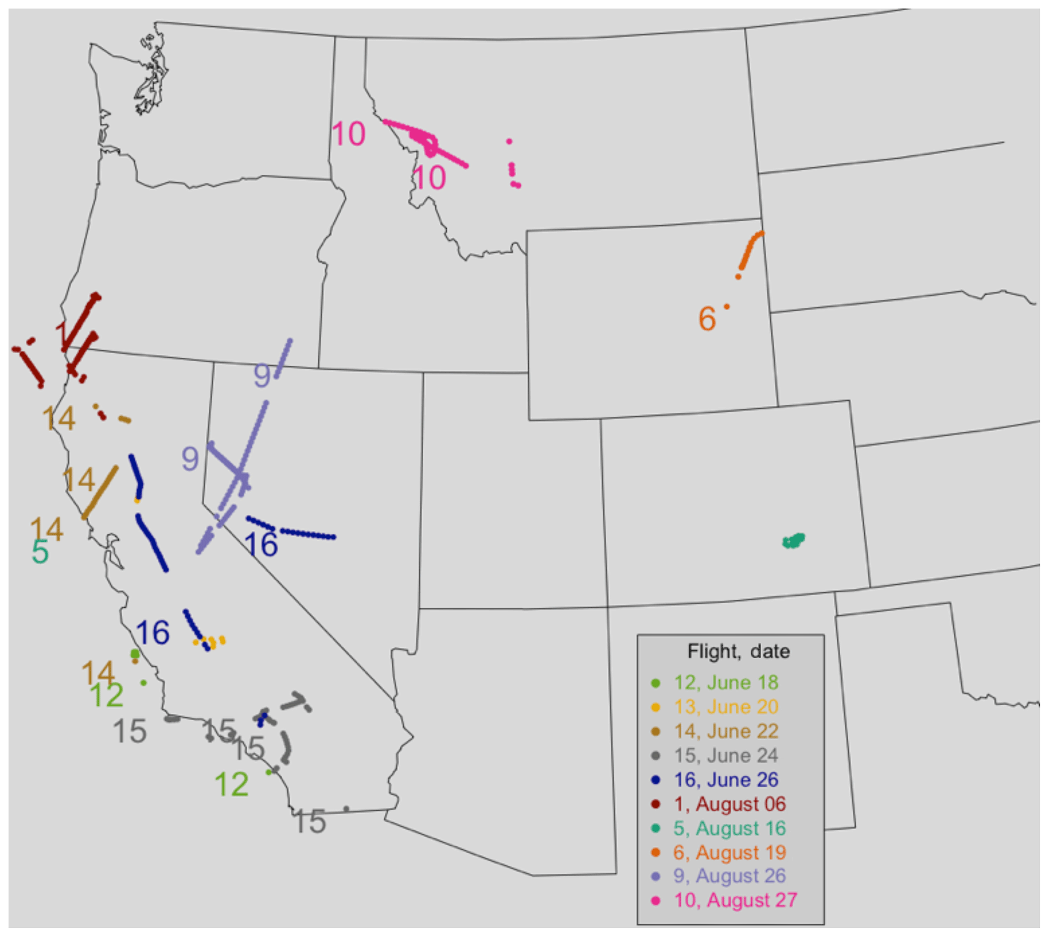
Figure 1 ARCTAS and SEAC4RS flights analyzed in this work. Each flight is identified by the flight number of that series. Flights 5 and 6 were in the Western USA but not included.

Flight tracks for the period and locations of major fires during these periods are shown in Fig. 1. Analysis of the vertical variation in fire tracers suggested that plumes below 5 km a.s.l. included recent and informative fires in our study. We saw no unequivocal variation in composition with height, possibly due to limitations on aircraft maneuvers low and near the fires. Consequently, the aircraft samples likely cannot adequately represent ground-hugging smoke flows.

1.2 Development of EF estimation to date

EnRs and EFs for biomass-burning plumes have largely been based on measurements of the CO₂ or CO concentrations in the plumes. Typical analyses begin with measurements of C_tot and the concentrations of several tracers we may call y_j: $j=\mathrm{1},\mathrm{\dots },N_{\mathrm{Tracers}}$. Multiple instances, $i=\mathrm{1},\mathrm{\dots },N_{\mathrm{Instances}}$, are observed, e.g., every few seconds or few minutes within a plume. An affine dependence (linear polynomial relationship including an intercept) is observed between each of the tracers and C_tot with a y intercept that depends most significantly on the local out-of-plume background values of CO₂, CO, and each tracer individually.

$$\begin{array}{}\text{(3)}& C_{\mathrm{tot}}=C_{\mathrm{bkgd}}+C_{\mathrm{burn}}\end{array}$$

The following analysis suggests several complexities that must be addressed in order to understand these affine relationships. Several aspects of slopes, intercepts, and deviations from linearity of the relationship of tracer y_j to C_tot plots must be examined, and so we transition to graphic terminology with x representing C_tot. Later we will describe measurements of C_tot and tracers j at a given instance i, x_i and y_ij. For a simple plume within a homogeneous mixed layer characterized by an x concentration x⁰ and y concentration y^E, we write

$$\begin{array}{}\text{(4)}& x=x^{\mathrm{0}}+\left(x-x^{\mathrm{0}}\right)\end{array}$$

and

$$\begin{array}{}\text{(5)}& \left(y_j-y_j^{\mathrm{E}}\right)=a_j\left(x-x^{\mathrm{0}}\right),\end{array}$$

with an enhancement ratio, a_j, that can yield EnRs directly. Early estimations (e.g., Greenberg et al., 1984; Andreae et al., 1988) used plots and regressions against CO₂ to estimate EnRs and EFs. These earliest techniques assumed fire was the main origin of CO₂. Very early it was recognized that other effects, e.g., variation in photosynthesis, respiration, and mixing, required a more sophisticated approach (e.g., Guyon et al., 2005). Alternatively (e.g., Andreae et al., 1988; Hobbs et al., 2003; Lefer et al., 1994), EnRs were derived with respect to CO. Symbolically,

$$\begin{array}{rl}\mathrm{EnR}\mathrm{estimate}& =\mathrm{Estimate}\stackrel{\mathrm{‾}}{\left({\displaystyle \frac{\mathit{\delta }{y}_J}{\mathit{\delta }\mathrm{CO}}}\right)}\cdot \mathrm{Estimate}\stackrel{\mathrm{‾}}{\left({\displaystyle \frac{\mathit{\delta }\mathrm{CO}}{\mathit{\delta }{\mathrm{CO}}_{\mathrm{2}}+\mathit{\delta }\mathrm{CO}}}\right)}\\ & =\left(\text{Regression slope of }{y}_i\text{ on }\mathrm{CO}\right)\\ & \cdot \left(\text{Regression slope of }\mathrm{CO}\text{ on }\right({\mathrm{CO}}_{\mathrm{2}}+\mathrm{CO}\left)\right).\end{array}$$

Here we use the symbol δ to indicate that these differences are evaluated from sequential samples or a regression of such a sequence. The second factor is based on the modified combustion efficiency (MCE),

$$\begin{array}{}\text{(6)}& \begin{array}{rl}\mathrm{MCE}& =\mathit{\delta }{\mathrm{CO}}_{\mathrm{2}}/\left(\mathit{\delta }{\mathrm{CO}}_{\mathrm{2}}+\mathit{\delta }\mathrm{CO}\right)\\ & =\mathrm{1}-\mathit{\delta }\mathrm{CO}/\left(\mathit{\delta }{\mathrm{CO}}_{\mathrm{2}}+\mathit{\delta }\mathrm{CO}\right)\\ & =\mathrm{1}-{\mathrm{EnR}}_{\mathrm{CO}},\end{array}\end{array}$$

with an attempt to estimate the domain of points for which a constant MCE could be assumed. The form of the difference symbol is written so as to emphasize that the differences are typically taken from a contiguously sampled time series of observations.

The method has become known as the normalized excess mixing ratio (NEMR) method (Akagi et al., 2011). Yokelson et al. (2013) described the care required to make sure that the MCE was well defined; otherwise, severe difficulties ensue. They describe a situation in which x⁰ and $y_{\mathrm{CO}}^{\mathrm{E}}$ in a diluting plume took on two distinct values, a mixed-layer value and a free-troposphere value, during plume rise and transport. More than two values may be relevant, emphasizing their call for a more thorough sampling of prefire air and its dilution environment. We describe below new methods to resolve many of the difficulties with x⁰ and to indicate unwanted effects of $y_{\mathrm{CO}}^{\mathrm{E}}$ variability. These methods could provide EnRs for many species with reasonable precision under more conditions.

This need for caution was very evident in the ARCTAS and SEAC4RS observational situations. Some Western USA data we analyzed showed variations in background $C_{\mathrm{tot}}={\mathrm{CO}}_{\mathrm{2}}+\mathrm{CO}$ (away from direct recent effects of respiration and photosynthesis) of 15 ppm (interquartile range of 4 ppm), while other Western USA regions showed variations of ∼ 8 ppm (according to the analyses in this paper that we present later in Fig. 4). The contributions from fires were often comparable to this variation, ∼ 2–40 ppm, mean ∼ 6 ppm. Air flowed from the west into forest fires at low altitudes or later diluted the smoke plume at intermediate levels. We could expect background air with a variety of histories of influence by photosynthesis (lower resultant CO₂) or respiration (higher CO₂), or we could expect urban-influenced air (higher CO₂). Low-level inflow air could have been mostly affected by local forests, farming, etc. Some of the most problematic situations tend to be associated with plumes sampled early in the day, when air from a nocturnal boundary layer – strongly enriched with respiration CO₂ – is mixed into the smoke plumes (Guyon et al., 2005). There could also have been substantial variations in C_tot due to intercontinental transport, the composition reflecting long-term previous modification due to these same processes and to latitudinal gradients. Yates et al. (2011) reported and more fully referenced atmospheric sampling of western air showing variations in CO₂ and also in CH₄ and O₃. On the east side of the Pacific anticyclone, the common pattern was for descent and horizontal-shearing displacements, producing substantial C_tot variations in both horizontal and vertical directions (Barry and Chorley, 1998).

Previous analyses have been made for the ARCTAS data, by Simpson et al. (2011) for the large Canadian fires sampled and by Hornbook et al. (2011) for all fires. The Hornbook article usefully complements this paper by describing features and origins of the plumes sampled. Both groups described novel methods but followed the traditional CO emissions ratio or NEMR methodology (Andreae et al., 1988; Hobbs et al., 2003; Akagi et al., 2011). Pfister et al. (2011) considered the emissions and transport of CO in the California ARCTAS samples. Analyses of the SEAC4RS fires have also been reported (Liu, 2017).

The following sections provide motivation for and understanding of an alternate approach to the description of EnRs and EFs, the mixed-effects regression emission technique, MERET; in some cases, MERET and the NEMR method may form complementary supporting views of plume emissions. Whereas the NEMR approach depends on multiple measurements in the same plume in an understood environment, MERET is typically applicable to individual measurements of similar EnR-determining fire conditions across many different plumes. It instead requires several informative fire tracer species, not simply CO₂ or CO, be measured simultaneously, as well as the tracer whose EnR is desired. It can also be used for good candidate EFs when the environmental history of the plume is not well characterized. It is applicable to any plumes encountered, without need for extensive measurement of that plume history.

MERET attempts to use the simultaneous variability, sample by sample, of a large set of fire tracer compounds and aerosol descriptors to find a single quantification, C_burn, of fire emissions, which it splits from C_bkgd such that the sum is C_tot. To do so, it must also ascribe a set of EnRs to the fire tracers and recognize that these EnRs may vary from sample to sample in a limited way. The interplay of these estimates contributing to C_burn and EnRs for each observation appears daunting. Section 3 will graphically illustrate how strongly effects beyond fire emissions describe variations in C_tot and also how similar and informative various tracers are as graphed against C_tot. Section 4 will describe a theory of multiple fire emissions co-emitted from a fire based on familiar plume concepts and give examples. The examples show the linearity of the theory that such simple approaches with a limited number of parameter estimates yield a reasonable approximation to more complex behavior. Sections 5 and 6 describe a mixed-effects regression algorithm based on plume theory. Section 7 provides a limited number of EnR estimates and describes graphically how flight segments describing similar emissions conditions can be identified.

2 Methodology – defining an indicator dataset

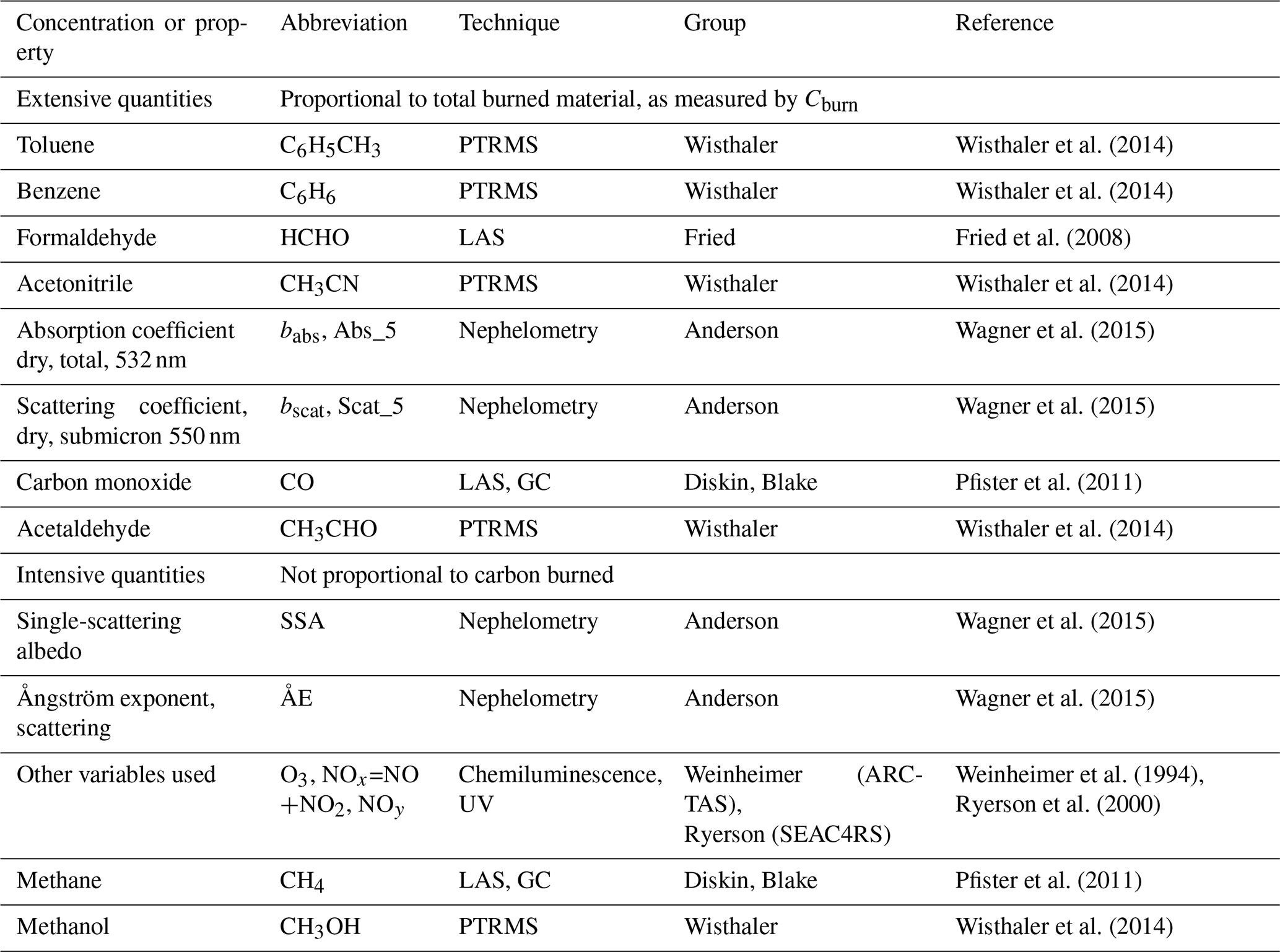
An initial task is the identification of tracers that are informative about burning and sampling rates. The technique we describe requires the measurement of $C_{\mathrm{tot}}\approx {\mathrm{CO}}_{\mathrm{2}}+\mathrm{CO}$ and several concentrations of emitted species or similar, extensive, properties of emissions (e.g., dried-airstream scattering coefficients, b_scat), which we will call emission indicator species or tracers. A set of indicator species was chosen for this publication to enable deriving relevant EnRs and to support our initial classification (e.g., flaming, smoldering, high-N fuel). It is important to have as many differently behaving emission indicator species as possible, as different indicators may respond differently to different fuels and fire intensities (“fire chemistries”), and such variations are usually not known before analysis. We favored indicator species with rapid sampling rates, so as to define C_burn for the maximum number of instances, but certain variables like CO, CH₄, and b_scat had special claims, as they can be maximally expressed in important types of fires. For our samples, methane and methanol showed significant idiosyncracies. Their cumulative probability distribution differed from all other tracers, with prominently very high concentrations and much higher positive skewness. We surmise that this behavior resulted from other prominent sources, e.g. cattle raising, or that very long distance transport and long lifetimes caused very great nonfire sources, like CO₂. It was convenient to use these same frequently measured indicator variables to define C_burn and also for classification of fire chemistries. For classification, we added intensive variables, essentially ratios that should be physically independent of C_burn.

Table 1 Indicator variables.

Notes: PTRMS – proton transfer mass spectrometry; LAS – laser absorption spectrometry; 1−ϖ is the single-scatter co-albedo; likewise, CO is linked to 1 (modified combustion efficiency) so that all values extend upwards from 0. For CO₂ measurements, see text.

The emission indicator species that satisfied these requirements for both missions are shown in Table 1, along with references to the measurement techniques and observers. Only extensive quantities (proportional to C_burn) are used in this paper. CO₂ was measured by Stephanie Vay (ARCTAS) and Andreas Beyersdorff (SEAC4RS) using the AVOCET instrument (Vay et al., 2011). In examining EnRs for various species, we also use the organic aerosol (OA) measurements (Wagner et al., 2015). ARCTAS and SEAC4RS data sites give full information, as instrumentation characteristics naturally vary somewhat between missions (https://www-air.larc.nasa.gov/cgi-bin/ArcView/arctas, last access: 12 August 2020; https://www-air.larc.nasa.gov/cgi-bin/ArcView/seac4rs?DC8=1, last access: 12 August 2020).

Our techniques use algorithms that currently allow few missing observations among the variables. The sampling rates for emission indicators measured by PTRMS (proton-transfer ionization mass spectrometry) differed between the two aircraft missions. The SEAC4RS mission acquired suitably complete PTRMS-derived datasets at a 1 min⁻¹ rate, and this defined the data interval used for both datasets. Additionally, in SEAC4RS CO was measured only by (less frequent) can samples for the first flights prior to the Rim Fire of 26 August 2013, and CH₄ was sampled only by cans for all flights. These are important species: CO is the most commonly used tracer for fire plumes because of its favorable plume-to-background concentration ratio and readily available measurement instrumentation. It is also used to define the MCE in much of the biomass-burning literature (Yokelson et al., 1996; Jaffe and Widger, 2011). Consequently, SEAC4RS imposed additional difficulties and processing. However, we judged it important to include SEAC4RS in a combined analysis to broaden the fire chemistries analyzed, as the Rim Fire was exceptionally large, hot, and well sampled.

The selection of fire plumes required some care. While CH₃CN is a highly specific tracer of fires (Singh et al., 2012), detailed analysis suggests that it is not the best quantitative tracer. (Further analysis suggested that CH₃CN has variable EFs, so it signals fires well but does not quantify C_burn adequately.) Plumes were characterized by levels of CH₃CN above 0.225 ppb, over 4 times the assumed background of 0.054 ppb. Since some plumes are known to be quite low in gas-phase emissions, a few samples with lower CH₃CN mixing ratios but with $b_{\mathrm{scat}}>\mathrm{2}\times {\mathrm{10}}^{-\mathrm{2}}$ were allowed in. Plots of CH₃CN vs. b_scat suggested that a linear combination of the two minimal conditions clearly separated a population of forest fire plumes from other high-particulate situations.

There were forest fire plumes for which urban sources of CO and other fire tracers made attribution and quantification problematic, and so a further test based on CO was applied to exclude urban samples, using CO vs. CO₂ plots for the years 2008 and 2013 separately (Fig. 2). We used a ΔCO∕ΔCO₂ ratio of < 33 ppb ppm⁻¹ to exclude plumes with excessive urban contamination. The figure suggests that some plumes with modest levels of urban influence remained and a few genuinely uncertain situations were excluded where fire might still have been dominant.

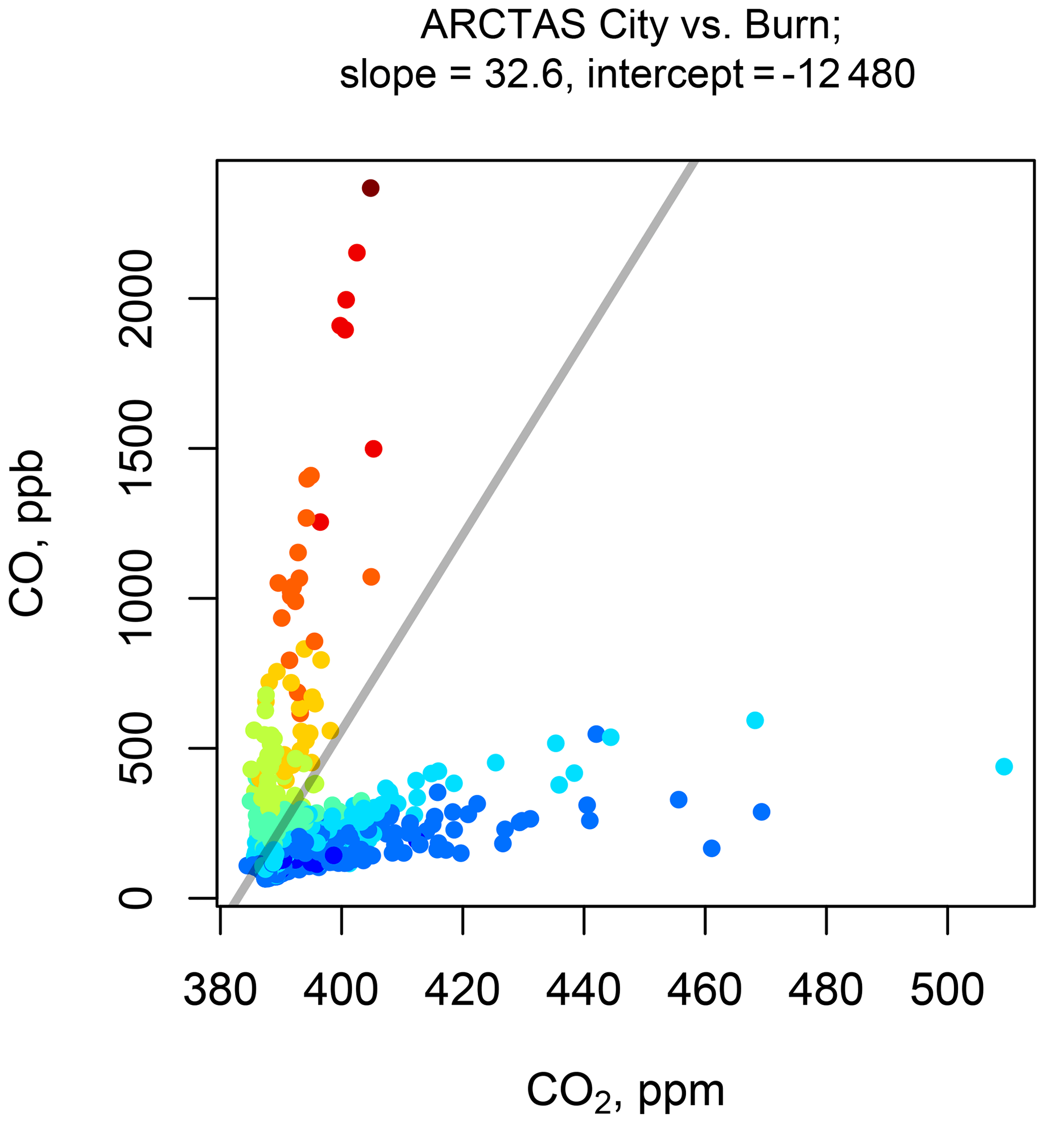
Figure 2 Urban and forest fire plumes are separable by the ratio of CO to CO2. Colors indicate a relative measure of CH₃CN above the background, from blue (lowest, ∼ 0.1 ppb) to red (highest, ∼ 6 ppb) values. The straight gray line indicates our selected discrimination between nonurban and urban.

Species with sources other than biomass burning and with lifetimes sufficiently long to allow regional mixing can pose difficulties somewhat similar to CO₂ variability, with solutions suggested in Sect. 8.2. We noted some localized observations of perplexing, consistently negative ΔCH₄∕ΔC_tot relationships in the ARCTAS data (but not other species) and removed these observation instances. Such relationships were found close to seaports or oil-producing regions.

3 Observed behavior of C_tot in fire plumes – properties of tracers

This section provides some examples of C_tot and fire tracers. It illustrates the limitations of changes in C_tot along a sampling path as an indicator of fire influence, C_burn, for emissions estimation and the much greater similarities of the variations in tracers that possess shorter transformation time-scales. These define our approach to EnRs and EFs. The relation of fire emissions to observed C_tot to C_burn can be apparently simple or complex, depending on how the history of nonfire CO and CO₂ entrained into fire plume air parcels affects C_tot. We show this commonality of relationships to motivate the theory of expanding plumes in Sect. 4. The theory suggests a regression relationship in Sects. 5 and 6, which applied, yields results in Sect. 7 that define relatively precise estimates of C_bkgd, C_burn, and thus EnRs.

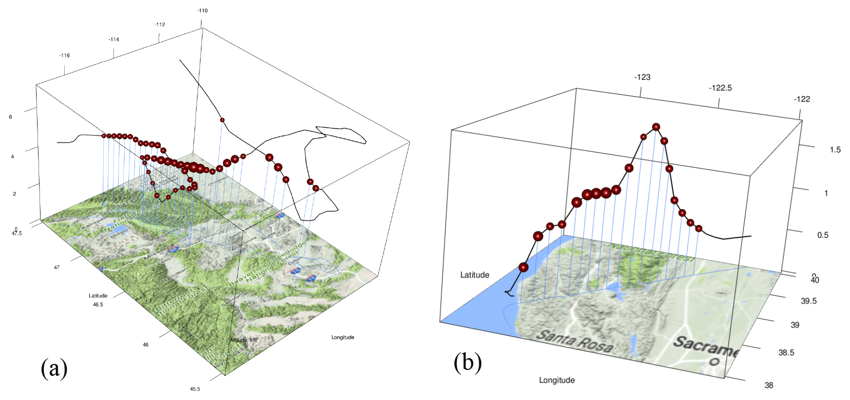
Figure 3 Flight paths and locations of plumes for two fire samples. (a) Sampling over Montana during SEAC4RS Flight 10. (b) Sampling in a cross-mountain transect along the Northern California coast. The size of the spheres indicates the relative amount of biomass-burning contribution. Numerical values of the contribution are in a later figure, Fig. 10. Some of the information was converted from © Google Maps using the R programming language.

Figure 3 describes two flights in which plume encounters show how the interpretation of $C_{\mathrm{tot}}=C_{\mathrm{burn}}+C_{\mathrm{bkgd}}$ can be simple or complex. Figure 3a shows the locations of the plume samples observed during SEAC4RS Flight 10 over Montana between 2 and 4.5 km a.m.s.l. Local topography ranged from 1 to 2 km elevation. This dataset included samples from the very intense plume of the Rim Fire (discussed later), collected far downwind. Figure 3b shows ARCTAS Flight 14, which was over the coastal mountains of Northern California at 0.5 to 1.5 km altitude, with topography from 0 to 1 km.

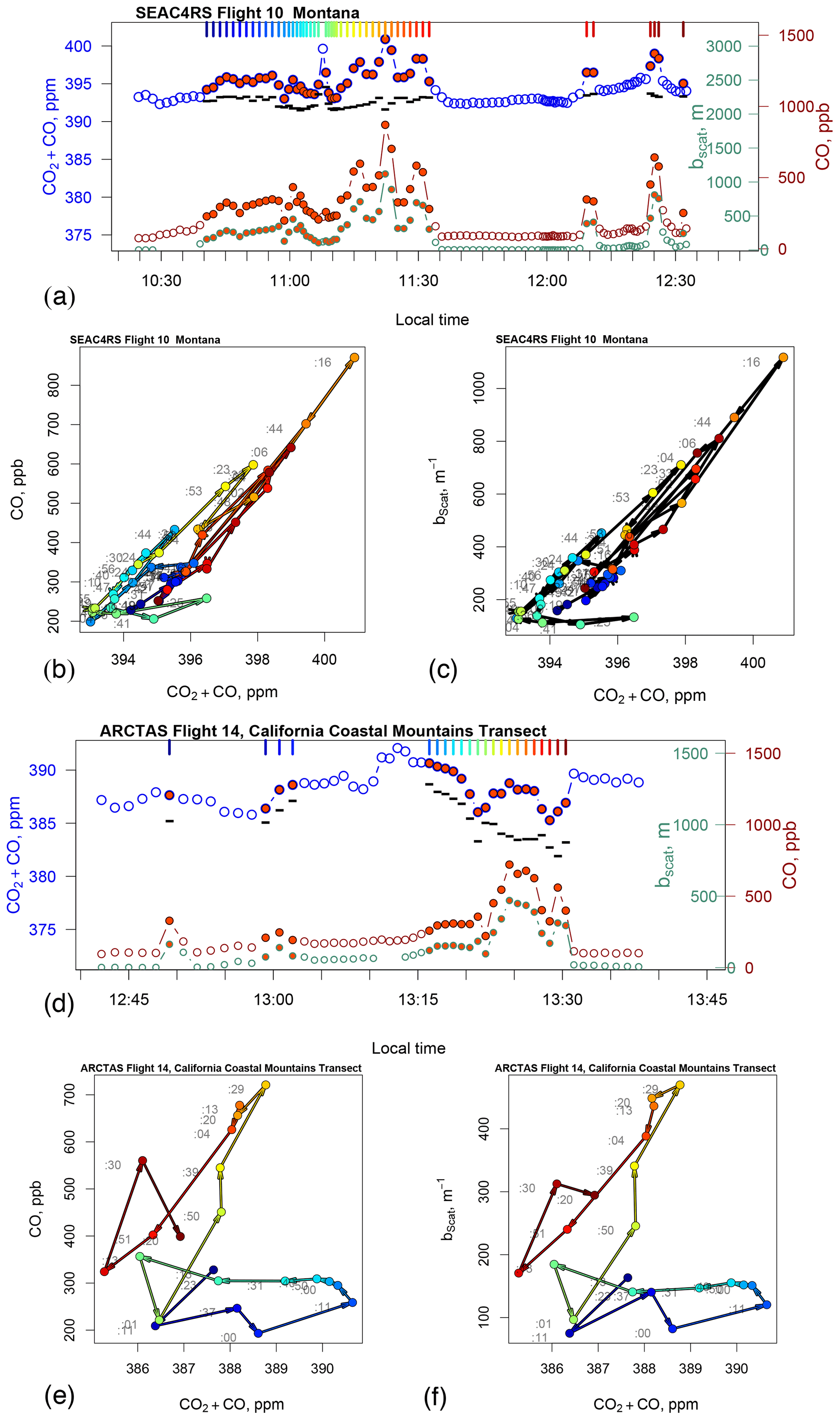
Figure 4 (a) Timeline of sampling, for the period shown in Fig. 3a, Montana, of CO₂ + CO (blue, left axis) and the fire tracers CO and b_scat (red and green points, right axis). Orange-filled points were identified as clear plume points. Unfilled points were not identified as such but might have some fire influence, especially near plume points. (b) Scatter diagram of CO vs. CO₂ + CO with arrows showing the time progression of aircraft sampling of identified plume points. Colors provide a key to times shown in panel (a). Light gray numerals give observation times in minutes. (c) A similar diagram of b_scat vs. CO₂ + CO. Similar shapes of figures are noted in the text. (d) Timeline of sampling for the period shown in Fig. 3b, coastal transect. (e) Scatter diagram of CO vs. CO₂ + CO during the transect, like in panel (b). (f) A similar diagram of b_scat vs. CO₂ + CO for the coastal transect. The black bars graphed in panels (a) and (d) are estimates of nonfire-influenced C_bkgd; see text. They and the nonplume points suggest air mass changes in CO₂ + CO.

Figure 4a (whose sampling path is mapped in Fig. 3a) gives the time series of fire indicators from Flight 10. The fire tracers CO and b_scat appear generally well correlated with C_tot. This correlation is seen in Fig. 4b–c. Colors from blue to red give a key to sampling times. The large orange dots in Fig. 4a and d distinguish the plume points selected (based on our plume tracers) from adjacent nonplume measurements made in the flight. The lines connecting the adjacent plume samples suggest two or perhaps three linear patterns pointing back to a no-fire background of C_tot ∼ 392.5 and 394.5 ppm. Separately, a few points near the horizontal axis seem to suggest a low EnR. These points occur in the middle of sampling, just after 11:00 LT. Patterns of variation related to b_scat (550 nm, Fig. 4c) are very similar to those of CO (Fig. 4b). Most plumes encountered suggest very similar slopes.

Whereas the SEAC4RS data in Fig. 4a–c suggest mostly expected behavior, the ARCTAS Flight 14 measurements (Fig. 4d–f) show that C_tot variations, likely due to C_bkgd variability, can greatly complicate the attempt to estimate EnRs. The very first samples plotted and those after about 13:35 LT have very clean tracer levels. (Those between 13:03 and 13:15 LT did not quite qualify as plume points, but the tracers do indicate some fire influence.) In this case, the trace of C_tot does not reflect fire influence well at all. Both fire tracers shown in Fig. 4d–f show wildly varying relationships to C_tot but are remarkably similar to each other in those relationships.

To conclude this section, we emphasize that variations in C_bkgd do occur unexpectedly in many apparently homogeneous datasets. The lines composed of small black bars in both Fig. 4a and d use our results of Sect. 7; they are estimates of C_bkgd for the selected fire plume cases. The patterns in Fig. 4 are given as plausible descriptions; the aim of this work is to support these with a uniform theory. For example, C_tot sampled by the airplane increases due to higher nonfire C_bkgd from just before 13:00 to 13:15 LT and then decreases gradually until about 13:28 LT. At one sample around 13:21 LT and several at 13:20–13:30 LT, the background is particularly low, 382–383 ppm. This is a plausible description of the mixing of air masses with original concentrations of C_tot of ∼ 382 and ∼ 388 ppm. Wisps of less-mixed air occasionally interrupt a relatively continuing trend. A close examination of the CO and b_scat increments compared to C_tot increments in Fig. 4d–f agrees with this description suggested by the black dashes. The simpler case of SEAC4RS Flight 10 shows a similar example. At 11:08 LST, early in the flight, there is a brief excursion upwards of C_tot without any excursion in the tracers. The small black bars show this as a plausible excursion of C_bkgd. Figure 4b and c show this as the two to three exceptional points, colored green, near the horizontal axis.

The plausibility of these examples highlights ideas of fundamental similarities in the way plumes of different tracers behave with entrainment even as C_bkgd varies in response to distant, unrelated processes, as seen in Fig. 4a. This leads us to a mathematical description of our observations in Sect. 4.

4 Theory – expanding plume for several species

4.1 A general relationship

Figure 5 gives a general description of the dilution process, showing by the size of cubes how a mole of near-flame air is diluted by nonfire material as entrainment occurs. (The boxes shown suggest volumes, but lofting adiabatically changes volume. Discussion in terms of moles simplifies the discussion of mixing ratios and EnRs.) The figure is based on observations of plume size and plume dilution during rising followed by largely horizontal dilution downwind (Lareau and Clements, 2017; Hanna et al., 1982), which are consistent with mixing ratios measured in this dataset and near-fire CO₂ concentrations of 1–2.5 ×10⁴ ppm. The sizes are meant to be suggestive, but we found that they give a valuable frame of discussion for all lofted forest fire plumes. Some details are in the Supplement, “Note on Volumes”.

Figure 5 Inflow of air into an expanding fire plume; a likely near-fire aircraft sampling location would be near the cube on the upper right. Cubes are shown with 3-D sizes proportional to the number of moles of entrained air. These may be considered volumes of air adjusted downwards to compensate for the adiabatic expansion that rising plumes undergo. The smallest cube is taken to be near the flames, at roughly the point where fire emissions transition from mixing to entraining background air. Exact placement of this cube is not important to the analysis of entrainment, expansion, and tracer mixing ratio. Successively larger cubes have volumes roughly in the ratio of 1, 40 (partially raised), and 140 (near-neutral buoyancy level); sizes are consistent with a buoyant fire plume (Lareau and Clements, 2017). The rightmost cube has a ratio to the first of 400, consistent with horizontal Gaussian dispersion during travel downwind. See text for more details.

Using Fig. 5 as a guide, consider a parcel originating at a time t₁ containing ν=ν₁ moles that expands with an exponential relative rate $r_{\mathit{\nu }}={\mathit{\nu }}^{-\mathrm{1}}(\mathrm{d}\mathit{\nu }/\mathrm{d}t)$. (For our illustrative examples and to rationalize the MERET method, we need not start at the flame. We suggest a reasonable starting point described below.) This rate of expansion r_ν(t) of the molar volume varies considerably over time, and fires are expected to have different magnitudes. Then molar mixing ratios will evolve with a law:

$$\begin{array}{}\text{(7a)}& {\displaystyle \frac{\mathrm{d}x}{\mathrm{d}t}}=-{\displaystyle \frac{\mathrm{1}}{\mathit{\nu }}}{\displaystyle \frac{\mathrm{d}\mathit{\nu }}{\mathrm{d}t}}\left(x-x^{\mathrm{E}}\right),\text{(7b)}& {\displaystyle \frac{\mathrm{d}{y}_j}{\mathrm{d}t}}=-{\displaystyle \frac{\mathrm{1}}{\mathit{\nu }}}{\displaystyle \frac{\mathrm{d}\mathit{\nu }}{\mathrm{d}t}}\left(y_j-y_j^{\mathrm{E}}\right),\end{array}$$

where x^E is the mixing ratio of entraining C_tot and $y_j^{\mathrm{E}}$ is the entraining background mixing ratio of fire tracer species or property j. (The term x^E here is later called x⁰ with a more general significance for possibly varying entrainment behavior.) The effect of volume addition is captured by ν(t) which varies with time and expansion. The use of the relative rate ν(t) does not require that the dilution is exactly exponential but does make the algebra somewhat simpler.

What happens when there are variable values of x^E(t) from fire to sampling point, for example in the boundary layer and free troposphere? Using τ to describe the integration through time of an expanding parcel,

$$\begin{array}{}\text{(8)}& \begin{array}{rl}{y}_j\left(t_{\mathrm{Sample}}\right)& =\underset{\mathrm{0}}{\overset{t_{\mathrm{Sample}}}{\int }}-\mathit{\nu }\left(\mathit{\tau }\right)\left(y_j\left(\mathit{\tau }\right)-y_j^{\mathrm{E}}\left(\mathit{\tau }\right)\right)\mathrm{d}\mathit{\tau }\\ & +y_j(t=\mathrm{0}),\end{array}\end{array}$$

with a similar equation for C_tot, which can be called x(t_Sample). It involves x(τ) and x^E(τ), where x(t=0) and y_j(t=0). These are determined by the C_burn from the fuel consumed and the tracer compounds released at the same time, as well as by background concentration, C_bkgd, and preflame backgrounds of the tracer $y_j^{\mathrm{E}}$. We leave aside as a separate problem for a fire-burning model the complexities of the actual flame and its incorporation of additional air. Our point t=0 is when entrainment of nonburning air becomes dominant.

Given the realities of atmospheric sampling, we must avoid describing the complete history of ν(τ) and any complex variation in x^E(τ) and $y_j^{\mathrm{E}}\left(\mathit{\tau }\right)$. This would require a complete description of air along the parcel trajectory and the turbulent physics of entrainment. Rather, we provide simple illustrations showing how generally the entrainment process affects both x(τ) and all the y_j(τ) values in the same proportions. This is a single-parcel description ignoring complexities of the rest of the plume. For convenience of discussion, we will describe cases in which the environmental air entrained has one or two values each of x^E(τ) and $y_j^{\mathrm{E}}\left(\mathit{\tau }\right)$ that are constant over long periods. For example, the background concentration of x^E=C_tot often has one value in the mixed layer and a different value above the mixed layer, potentially taking on several values in several layers. The same is true for the fire tracers y^E. Conceptually there may be several regions which contribute; the exact history is lost. Our idea is that regression analysis allows us to infer a characteristic sum of effects which is described by a single quantity. The analysis can only be as complex as the number of our measured quantities allows. See also Supplement, “Note on Initial Point”.

Table 2 Table of symbols.

^∗ Note that symbols may transition from hypothetical to estimated as the discussion develops.

Returning to the differential-equation view of the simple expanding plume model, we see a method for estimating the most important parameters. Solving each of the equations for the expansion rate and equating the expressions, we obtain a form that eliminates the details of entrainment and emphasizes proportionality. We recommend the reader to refer to Table 2 during the discussion of theory and then the discussion of estimation details.

$$\begin{array}{}\text{(9)}& {\displaystyle \frac{\mathrm{1}}{\left(y_j-y_j^{\mathrm{E}}\right)}}{\displaystyle \frac{\mathrm{d}{y}_j}{\mathrm{d}t}}=-{\displaystyle \frac{\mathrm{1}}{\mathit{\nu }}}{\displaystyle \frac{\mathrm{d}\mathit{\nu }}{\mathrm{d}t}}={\displaystyle \frac{\mathrm{1}}{\left(x-x^{\mathrm{E}}\right)}}{\displaystyle \frac{\mathrm{d}x}{\mathrm{d}t}}\end{array}$$

Since $\mathrm{d}{y}_j^{\mathrm{E}}/\mathrm{d}t=\mathrm{0}=\mathrm{d}{x}^{\mathrm{E}}/\mathrm{d}t$ , we get

$$\begin{array}{}\text{(10)}& {\displaystyle }\ln \left(y_j-y_j^{\mathrm{E}}\right)=\ln \left(x-x^{\mathrm{E}}\right)+C_j,\text{(11)}& {\displaystyle }\left(y_j-y_j^{\mathrm{E}}\right)=a_j\left(x-x^{\mathrm{E}}\right)a_j=\exp \left(C_j\right).\end{array}$$

Note that by our definitions, the reasonable interpretation of C_j is the EnR a_j for species j.

Consider two observations of the same plume, each made at differing degrees of dilution ν. For convenience, these are labeled β and α, mnemonically “before” and “after.” Temporally they could be nearly coincident or β could come after α.

$$\begin{array}{}\text{(12)}& \begin{array}{rl}\left(y_{\mathit{\alpha }j}-y_{\mathit{\beta }j}\right)& -\left(y_j^{\mathrm{E}\mathit{\alpha }}-y_j^{\mathrm{E}\mathit{\beta }}\right)=\\ & a_j\left(x_{\mathit{\beta }}-x_{\mathit{\alpha }}\right)-a_j\left(x^{\mathrm{E}\mathit{\alpha }}-x^{\mathrm{E}\mathit{\beta }}\right),\end{array}\end{array}$$

for periods of expansion in which the entrained concentrations are constant. See also Supplement, “Note on Varying Entrainment”.

This formula is the basis for the NEMR technique mentioned above, with j=CO playing a particularly important role. The inequality restrictions should be evaluated for an EnR to be a candidate for an ER and then an EF. In some cases, the background values, x^Ea and $y_j^{\mathrm{E}a}$, might be estimated from measurements made outside the plume. It can be somewhat more difficult to estimate x^Eb and $y_j^{\mathrm{E}b}$ upwind of the source, especially for air entraining into the fire plume at its source. A plume may also entrain air from various backgrounds and at various times during lofting and spread. That is, the history of entrainment may well be more complex than two conditions, “a” and “b”, and the number of situations where we may estimate EnRs and then EFs is greatly limited. This important realization was described by Yokelson et al. (2013). The NEMR method can deal with most differences in x^Eb but not in $y_j^{\mathrm{E}b}$ for most tracers, and the quantity $y_{\mathrm{CO}}^{\mathrm{E}b}$ for carbon monoxide must be well sampled and well understood.

4.2 Examples showing robustness of computations of idealized C_tot

We used this approach to produce the following concrete examples of increasing complexity. They illustrate the origin of the features seen in Fig. 6 in terms of this simple plume dilution model. They helped motivate our solution techniques and indicate methods of analysis of individual plumes. These examples indicate possible limitations, but they also indicate a comforting averaging behavior of the linear differential equations as they describe our solutions. These uniformities and deviations also showed up in the analyses that we develop below. The examples also give some quantitative feel for the effects of deviations from the simplest hypothesis; e.g., x^E and $y_j^{\mathrm{E}}$ remain constant through time. Fig. 6 shows calculations describing behaviors of x and y_j in several plausible situations. Each graph represents the development of plume mixing ratios for a period of plume doubling, similar to the analysis time chosen in Poppe et al. (1998), following their equations, Eqs. (7) and (8). The dots show equal increments of plume expansion. Most parameters defining the equations may be read from the graphs themselves. Each initial concentration is shown by the points to the upper right of the line, i.e., the points with maximum x=C_burn and y_j= tracer concentration for each case considered.

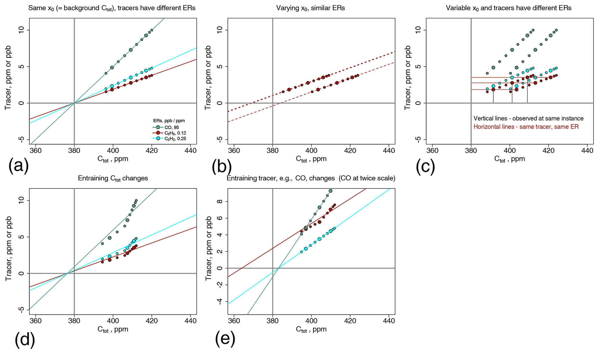
Figure 6 (a) Simulated dilution of three different fire tracers' EnRs as shown, and with environmental x^E of 380 ppm. These are nominally CO, benzene, and ethylene. Background concentrations of the tracers have been subtracted. C_burn is measured from the y axis, where C_tot has the value of 380 ppm. Larger dots highlight equivalent degrees of dilution. (b) Simulated dilution of one tracer, nominally CO above background, with different background x^E. Backgrounds are illustrated by the x intercepts. (c) Simulation of three tracers, varying EnRs and varying backgrounds (deducible from the x intercepts). Thin lines emphasize similar constant y values with different backgrounds and constant x⁰ values with varying EnRs. (d) Simulations like in panel (a) but with a change in the x^E entrained x⁰=C_burn background from 395 to 375 ppm at the time of the eighth dilution step. A single applicable background value of ∼ 378 ppm is a linear interpolation between 395 and 375 ppm. (e) Simulation where background x^E remains constant but background CO changes by 1.5 ppb during the same time (CO drawn at twice the height for visibility).

Figure 6a illustrates a plume history for x^E=380 ppm and EnRs with respect to airborne C_tot of 95 $\times {\mathrm{10}}^{-\mathrm{3}}$, 12 $\times {\mathrm{10}}^{-\mathrm{6}}$, and 25 $\times {\mathrm{10}}^{-\mathrm{6}}$ ppm ppm⁻¹, which are reasonable values for carbon monoxide (in ppb), benzene, and ethylene (in ppt). In the figures, focus attention on the relative behavior of the tracers. It is assumed that there are no consequential production or destruction reactions and also that there is a constant background tracer concentration, which has been subtracted. The individual plots show situations of increasing complexity. Figure 6a shows the dilution behavior of the three species. A constant dilution rate is plotted; note that a varying dilution rate changes the spacing of the dots but not the linear pattern. Larger dots highlight an equivalent dilution of tracer and x=C_tot as would be observed in hypothesized discrete airplane samples. Figure 6b illustrates the dilution of CO in environments with differing entrained x^E. In Fig. 6a the larger dots align vertically; in Fig. 6b, they align horizontally. Figure 6c illustrates the situation where both EnRs and backgrounds vary; the thin lines emphasize independent aspects of EnR and x^E. The points on the x axis where (excess) tracer is zero are important to our estimation technique, more important than x^E. Estimation of x^E utilizes data on the vertical lines, while EnRs utilize information from both the vertical and the horizontal lines. Statistically speaking, the problem of estimation of both backgrounds and EnRs illustrates simultaneous effects that are “separable”. The reader may wish to extend the analysis to a large sequence of changes in entrained concentrations and note the essential linearity of this aspect of the formulation and that the solution expresses an appropriate averaging effect. We remark that the near uniqueness of the solutions obtained below (making small allowances for measurement error) will underline the robustness of the solutions.

However, the effect of uniform variations in background tracer concentrations $y_j^{\mathrm{E}}$ is not completely solved in this work. $y_j^{\mathrm{E}}$ can be estimated by examining the lowest values of $y_j^{\mathrm{E}}$ in nonplume air; it is best to exclude values that appear to have contributions of exotic air (e.g., stratospheric air) or possible measurement problems at very low mixing ratios (e.g., negative values). Some comments follow as we move towards the topic of estimating individual values from a large set of x_i values and y_ij values in a practical situation where we analyze instrumental data. Restricting attention to larger values of x_i and y_ij greatly ameliorates problems arising from $y_j^{\mathrm{E}}$.

5 Theory – a regression relationship for EnRs

Let us consider more broadly the equations that provide a basis for statistical estimation. For current purposes of explanation, we make the seemingly large assumption that points from different plumes have similar properties at the same degree of dilution and may be compared. That is, the a_j values are consistent for all plumes. Effects of varying x^E and $y_j^{\mathrm{E}}$ between the plumes may be largely taken out by regression; that is our current concern. Later, we will describe our approach to address possible variations in the EnR relationships a_j for parcels in the same or different plumes.

The basis of MERET utilizes the concept of the unmeasured extreme where y_aj=0. To begin with, we consider the situation where (i) the emissions relationships a_j are constant for all observations and (ii) background values of the tracers are small enough in a relative sense; i.e., $\left|y_j^{\mathrm{E}a}-y_j^{\mathrm{E}b}\right|\ll \left|y_{aj}-y_{bj}\right|$. That condition is common for many species that have loss timescales of less than a month and/or have small nonfire sources. Each of these restrictions can eventually be relaxed. In this case

$$\begin{array}{}\text{(13a)}& {\displaystyle }{y}_a=a_j\left(x_a-\left\{x_b-x^{\mathrm{E}b}+x^{\mathrm{E}a}\right\}\right)+y_j^{\mathrm{E}a}-y_j^{\mathrm{E}b},\text{(13b)}& {\displaystyle }\begin{array}{rl}& y_a=a_j\left(x_a-\left\{x_b-x^{\mathrm{E}b}+x^{\mathrm{E}a}\right\}\right),\\ & \text{for }\left|y_j^{\mathrm{E}a}-y_j^{\mathrm{E}b}\right|\ll \left|y_{aj}-y_{bj}\right|.\end{array}\end{array}$$

Notice that terms within braces can be estimated by regression as sums, varying by the situation b. What if the values of these terms change discretely in time, for example as a plume leaves a daytime mixed layer or distinct upper-air plumes are encountered? Simple algebra with linear formulas suggests that estimates of the terms in braces change discretely. Gradual changes in entrained mixing ratios of course imply a continuity condition on these terms.

We return to the illustrative dilution behaviors described in Fig. 6. Figure 6d describes a sudden change in background x^E by 20 ppm, x^Eb to x^Ea, midway in the expansion and dilution; at this stage of plume evolution, 20 ppm is about 4 times larger than typical fire contributions to C_tot. Estimates of $x_i^{\mathrm{0}}$ from a few samples along these lines (without knowledge of the time of change) would be intermediate. Equation (13) suggests that the EnR estimate need not be affected. Some similar calculations make it clear that the estimates average satisfactorily under varied assumptions. Figure 6e shows a very contrasting behavior, when there is a sudden change in concentration of entraining tracer (CO) during plume dilution, a change of 1.5 ppm. In comparison, the addition of CO by burning at the start of the interval is ∼ 3.5 ppm. We may distinguish this as ${\widehat{x}}_{ij}^{\mathrm{0}}$, where the j=CO and the hat indicates an estimate. This graph also suggests that if there are more than three tracers (we use eight), then the median of all the estimates, median (${\widehat{x}}_{ij}^{\mathrm{0}}$), is robust against errors resulting if a tracer j has a variable or poorly described background, resulting in ${\widehat{x}}_{ij}^{\mathrm{0}}$ at falling being distinctly higher or lower than the others. We must be concerned about this since tracers can have occasionally important nonfire sources. A small change in background of a tracer compared to observed change due to fire is critical in determining a useful estimate of the background x⁰ as well as in determining the quality of the EnR of a tracer. Methane in particular has a long atmospheric lifetime and several sources of similar strength; in California, livestock and fossil-fuel extraction significantly influence mixed-layer concentrations flowing into a fire updraft. Consequently, it can exhibit variations that are more than 10 % of the fire emission contribution for well-dispersed plumes.

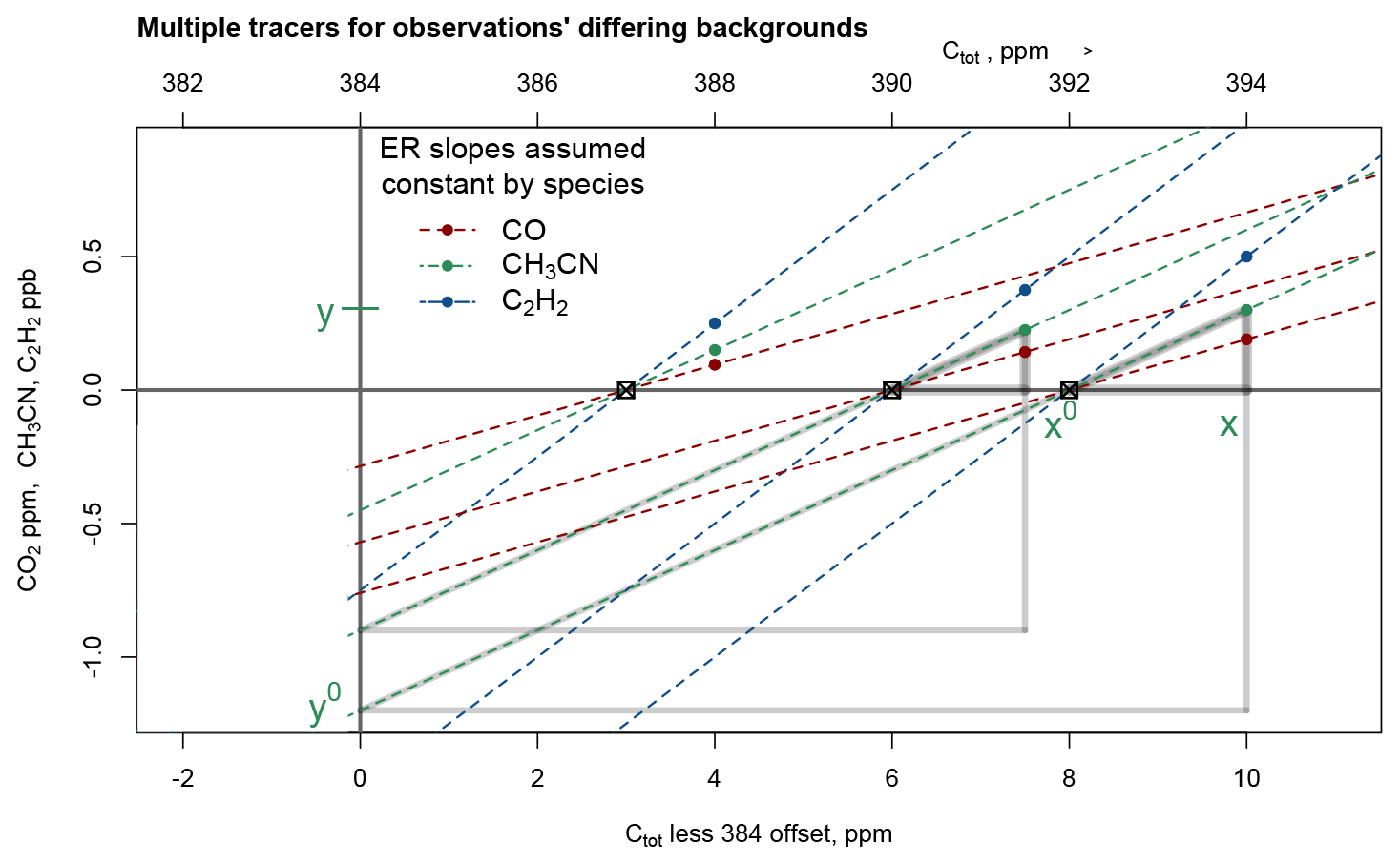
Figure 7 Multiple tracers allow a solution for an equivalent-background x⁰ value, illustrated by an idealized example largely replicating the conditions of fire plume sampling above an Amazonian mixed layer as described by Yokelson et al. (2013). The dashed colored lines indicate the theoretical response of tracer to the C_tot when C_bkgd takes on various values indicated by black squares. There are several lines showing the ideas expressed in Fig. 6a. The fact that the various colored lines associated with each x value meet at the value with x coordinate x⁰ and y coordinate 0 represents the estimation that precisely solves Eq. (5) above. If we had included error in observations or variation in EnRs, there would be variations in the positions of x⁰ and the slopes. As Sect. 6.1 describes, regression of tracer vs. C_tot is required and gives a spread of y intercepts. Nevertheless, these can be mapped back to x intercepts using slopes and the concept of similar triangles. The nested gray triangles illustrate this idea for each of two values of x⁰.

The preceding discussion suggests that we may use the specialized least-squares technique,

$$\begin{array}{}\text{(14)}& y_{ij}=a_j\left(x_i-x_i^{\mathrm{0}}\right)+e_{ij},\end{array}$$

where the x_i and the y_ij are observations of C_tot at an instance i and for the set of variables j at that instance i. Here $x_i^{\mathrm{0}}$ expresses several terms of Eq. (13) and any other corrections not proportional to a_j. We may call $x_i^{\mathrm{0}}$ an “effective background”. However, it is not a specific background but actually summarizes the whole effect of changes in C_bkgd and also the degree of dilution. This means that the regression can synthesize information from not just one well-characterized plume but also different plumes provided we expected them to have similar a_j behavior. Figure 7 illustrates the use of regression employing the ideas developed in Fig. 6. Using the same formulas as above, we depict observations of CO, C₆H₆, and C₂H₂ made at three instances (times). The three tracers determine a value x⁰, and given that information, the three tracer enhancements and therefore tracer EnRs are determinable. The nested gray triangles, similar triangles, illustrate this idea for each of the two values of x⁰ corresponding to two observation instances when it is assumed that x⁰ has changed. MERET uses the idea that the slopes must be equal. This simulation assumes no error in the measurements of CO₂ + CO or the tracers and assumes no variation in the EnRs, so values are determined perfectly.

How well are these situations with multiple observation instances and multiple tracers determined? In the case of two samples and two tracers, i.e., N_Instance=2 samples and N_Tracer=2 slopes (EnRs), we need to estimate x₁, x₂, a₁, a₂, and x₀ using only y₁₁, y₁₂, y₂₁, and y₂₂; there are not enough measured variables to determine a unique solution: $N_{\mathrm{Tracer}}+N_{\mathrm{Instance}}+\mathrm{1}>N_{\mathrm{Tracer}}\cdot N_{\mathrm{Instance}}$; viz., 5>4. However, if there are three tracers, $N_{\mathrm{Tracer}}\cdot N_{\mathrm{Instance}}>N_{\mathrm{Tracer}}+N_{\mathrm{Instance}}+\mathrm{1}$ and we get a solution. In this case, any measurement error, or indeed lack of perfect similarity in response slopes, can give somewhat conflicting solutions.

6 Methodology

6.1 Finding the CO₂ + CO background

The use of tracers with backgrounds removed and then scaled to a common mean establishes a well-conditioned matrix problem and easier analysis of sensitivity effects. We have identified forest fire plume samples and N_Tracer tracers whose background values can be reasonably estimated. Let us proceed with the regression and begin to address some complications that arise. The mathematical problem we must solve is Eq. (14), which we will rewrite to emphasize that we are starting in native units.

$$y_{ij}^{\mathrm{measured}}-y_j^{\mathrm{E}}=a_j\left(x_i-x_i^{\mathrm{0}}\right)+e_{ij}$$

In the following development in this section, we will work with y_ij above the background; i.e., set $y_{ij}^{\text{prenormalized}}\leftarrow (y_{ij}^{\mathrm{measured}}-y_j^{\mathrm{E}}$).

We must attempt to fit $y_{ij}^{\text{prenormalized}}$ for each species j (1 to N_j) and for each measurement instance i (1 to N_j). The term e_ij describes the error. Besides removing backgrounds, we wish each tracer j to contribute equally to the sum of squares that determines a regression, independent of the tracer's mean value. Consequently, we should normalize the tracers so that their mean is 1:

$$y_{ij}=y_{ij}^{\text{prenormalized}}/\underset{i}{\mathrm{mean}}\left(y_{ij}^{\text{prenormalized}}\right).$$

We will use normalized values of the tracers for the following development until Eq. (20). It is not necessary to normalize x_i, but it will be useful to subtract a baseline. This suggests that the basic regression equation might be the following:

$$\begin{array}{}\text{(15)}& y_{ij}=a_j\left(x_i-x_i^{\mathrm{0}}\right)+e_{ij}.\end{array}$$

Equation (15) also summarizes just why the determination of ERs is difficult: the equation is nonlinear in the multiple regression sense; i.e., we must include the mixed i and j term $a_j{x}_i^{\mathrm{0}}$ as a regression term. The problem is a mixed-effects model: we must estimate the statistics of two separately varying processes affecting $x_i^{\mathrm{0}}$ and a_j.

A complication arises concerning the use of regression. The fire tracer variable y_ij values must “point back” to a zero point, where no C was added by the burn, $C_{\mathrm{burn}}\equiv x_i-x_i^{\mathrm{0}}=\mathrm{0}$, but each instance i may have a different zero point. A regression formula should solve this in some way. Commonly, regression fits provide a y intercept, i.e., the value at x= 0. Here we have an x intercept to estimate, i.e., the concentration of the reference species at zero-added fire emissions, and so the problem becomes nonlinear in the regression sense. In summary, we have a nonlinear random-effects model (Pinheiro and Bates, 2000; Gajoux and Seoighe, 2010; Bates et al., 2014; Gajoux, 2014), which requires specialized techniques.

One feature of Eq. (15) is emphasized: the formulation does not require any relationship of x_i or y_ij in time; instances must only represent a sufficiently coherent class of fires. One would expect more accuracy and discernment of features in similar forest fires but not in forest fires and grass fires. For the latter case, the assumption of consistent a_j becomes problematic.

Why not simply reverse the problem and seek x as a function of y?

$$\begin{array}{}\text{(16)}& x_i={\mathit{\alpha }}_j{y}_{ij}-x_i^{\mathrm{0}}+e_{ij},\end{array}$$

where $x_i^{\mathrm{0}}$ values are estimated with a regression model (specifically a fixed-effects model). The difficulty is that the trivial solution $x_i=-x_i^{\mathrm{0}}$ fits perfectly and was hard for us to avoid even when we attempted to restrict the solution with a nonlinear solver. Is it not easier to convert y intercepts into x intercepts? This appears more productive and should appeal to those not familiar with using a nonlinear solver in this particular mode of nonlinearity. In place of Eq. (15), we may write a regression equation with an intercept:

$$\begin{array}{}\text{(17)}& \mathrm{Regress}{y}_{ij}=a_j{x}_i+c_i^{\mathrm{0}}+e_{ij},\end{array}$$

where the y intercepts, $c_i^{\mathrm{0}}$ values, are estimated for each instance and the e_ij values are minimized by least squares. The R expression used to solve this problem was main.lmer = lmer( y ∼ x + ( x - 1 | species.type ) + ( 1 | id ) + 1), where id indicates the sequential observation number for the tracer species. The term species.type indicates the species description j. The word type signals a generalization described in the next section. (This expression is written in a commonly used Wilkinson–Rogers symbolic form: the symbol ∼ describes our intention to make a regression estimate; Wilkinson and Rogers, 1973. The vertical lines indicate how factors are involved with variables; 1 indicates an intercept is to be described by a random effect; and (x - 1 | species.type) indicates that a slope that multiplies x is to be estimated, indexed by species.type. “No intercept estimated” is signaled by −1.) The regression results generate a set of fitted y values which we may call ${\widehat{y}}_{ij}$ and a set of fitted ${\widehat{a}}_j$ values. Together, the values of x_i, ${\widehat{y}}_{ij}$, and ${\widehat{a}}_j$ imply a y intercept $y_{ij}^{\mathrm{0}}$ when x_i=0 as shown in Fig. 7. One evaluates the fit for x_i=0. Then one may use the slope estimate ${\widehat{a}}_j$ of a_j by regression to find the several estimates of ${\widehat{x}}_{ij}^{\mathrm{0}}$ provided by

$$\begin{array}{}\text{(18)}& {\widehat{x}}_{ij}^{\mathrm{0}}=\left({\widehat{y}}_{ij}-y_{ij}^{\mathrm{0}}\right)/{\widehat{a}}_j.\end{array}$$

This is where we use the similar-triangles concept of Fig. 7. The use of a single ${\widehat{a}}_j$ value for all observation instances of the same species (more precisely, species.type) is a strong constraint on the resulting estimate. This is how for ${\widehat{a}}_j$ and ${\widehat{x}}_{ij}^{\mathrm{0}}$ we use the concept of the similar triangles described in Fig. 7 of Sect. 5.

We then take

$$\begin{array}{}\text{(19)}& {\widehat{x}}_i^{\mathrm{0}}=\underset{j}{\mathrm{median}}{\widehat{x}}_{ij}^{\mathrm{0}}.\end{array}$$

The estimation of ${\widehat{x}}_i^{\mathrm{0}}$ now allows estimates of the incremental carbon liberated to the atmosphere, $C_{\mathrm{burn}}=\left(x_i-{\widehat{x}}_i^{\mathrm{0}}\right)$. We will drop the hat from ${\widehat{x}}_i^{\mathrm{0}}$ below, writing $x_i^{\mathrm{0}}$ and $C_{\mathrm{burn}}=\left(x_i-x_i^{\mathrm{0}}\right)$ except when we wish to emphasize their nature as estimates. Emission factors for individual-tracer species may be obtained directly by adding fixed and random effects on slopes for each species and each observation, ${\widehat{a}}_j$. An enhancement ratio for any concentration or property y_j with a background, measured at time i in the aircraft sampling, can be obtained using the carbon-burned estimate:

$$\begin{array}{}\text{(20)}& \begin{array}{rl}\mathrm{EnR}\mathrm{for}{y}_{ij}& ={\displaystyle \frac{\left(y_{ij}^{\mathrm{measured}}-y_j^{\mathrm{E}}\right)}{\left(x_i-x_i^{\mathrm{0}}\right)}}\\ & \equiv \left(y_{ij}-y_j^{\mathrm{E}}\right)/{\left(C_{\mathrm{burn}}\right)}_i.\end{array}\end{array}$$

To repeat, the variable y_ij now stands for any property for which we seek an EnR, for example ozone, which is not one of the eight indicator variables. $y_j^{\mathrm{E}}$ describes a non-fire-dependent background value. This ratio estimate is available for all tracers and is preferred over a similar slope variable ${\widehat{a}}_j$ used to estimate $x_i^{\mathrm{0}}$ in the in Eq. (18) above.

Formulas for the statistics of ratio quantities with uncertainties in the numerator and denominator can be theoretically complex, so we simply computed error estimates by simulation using computed Bernoulli trials. For both the numerator and the denominator, 1000 samples of normal distributions were calculated, using their uncertainties as 1σ values. Then the ratios of the first numerator and first denominator normal deviate sample, the second, …, the 1000th normal deviate sample for the numerator divided by the 1000th normal deviate sample were calculated, and the distribution of ratios was summarized. For the numerator, the measured value and the suggested standard deviation (typically a percentage ratio) provided the parameters for the normal distribution. For the denominator, the mean was the C_burn estimate, and the standard deviation was a value of 0.25 ppm, documented as the measurement error (precision + bias) of CO₂ (see Table 1). Uncertainties in the calculation of ${\widehat{x}}_i^{\mathrm{0}}$ were considered small and did not add to the dispersion of the denominator, especially since it is clear that any additive biases contributing to the quoted uncertainty in (CO₂ + CO) cancel out. Sample calculations in the Supplement (“Note on Sensitivity to Number of Tracers Used”) suggest errors typically of a magnitude of 0.03 ppm due to variations in technique and usually of < 0.1 ppm. Additive errors should also cancel out for the numerator, since a background is subtracted. Indeed, some tracers like ethene appeared to have a negative background as determined from plots and simple regression calculations of y_ij on (C_burn)_i. This is not unexpected, since these compounds are sampled into cans, where a small but self-limiting coating of the measured species on the can surfaces might cause such a negative offset, and yet the integrity of the can sample at larger values might be little affected.

6.2 Practicalities – variable EnRs

Equations (17)–(19) provide the basis of MERET. There are however some details that increase its relevance and accuracy. First there is normalization. Common practice is to normalize all the tracer species j with respect to the mean of all observations of species j, after subtracting a baseline. This allows each tracer to influence y_ij equally. Assigning weights accomplishes the same purpose, but scaling allows better diagnostic graphs. In fact, the literature referenced above emphasizes how informative j=CO is, despite its relatively small variation in EnR or slope. Consequently, we give CO twice the weight of all the other species.

Secondly, we allow for a certain amount of true variation in the EnRs, expecting this to make Eq. (18) perform better. This is done by imagining that virtual species can be associated with “fire types”, for example “flaming CO”, “smoldering CO”, or “high-nitrogen-fuel CH₃CN”. A fire type is a value for each observation that applies to all tracer species at that instance. It expresses commonalities between different mixes of burning emissions, commonalities that may be more frequently or less frequently expressed in any given plume, e.g., smoldering-CO fire type. We might speculate on the nature of the fire type, e.g., smoldering or derived from nitrogen-rich fuel. However, we let the statistical technique define these types and so apply basic clustering techniques. We used nonnegative matrix factorization (NMF), but Mahalanobis clustering or other techniques seem to do equally well. NMF and k-means clustering are shown to be equivalent in cases corresponding to our work (Ding et al., 2005). A larger number of cluster classes will allow more ability to follow the EnR actually characteristic of the observation but at the cost of parsimony and sensitivity to instrumental error for the species or property. We used the R routine nmf() with k=6 components and the Lee estimation technique with singular-value initialization (Lee and Seung, 2001; Boutsidis and Gallopoulos, 2008). Use of the singular-value option for initialization proved satisfactory; it agreed well with the default method.

Since all fire tracers are correlated, such clustering characterizations are much better defined if based on a rough normalization to the fuel burned. We used a consensus variable, composed from all the defining tracers, to act as an agent for constructing ratios:

$$\begin{array}{}\text{(21)}& {\mathit{\nu }}_i=\underset{j}{\mathrm{mean}}\left(y_{ij}\right).\end{array}$$

This ratioing variable plays a role logically played by $C_{\mathrm{burn}}=\left(x_i-x_i^{\mathrm{0}}\right)$. Exact quantitative calibration of C_burn in parts per million is not required, just a relative scale is. We found it could be intuitively helpful to conceive of the ratioing variable in parts per million of carbon, just as with our later estimate of C_burn. To assign parts-per-million values, see the Supplement, “Note on an Early Approximate C_burn”.

We end this section on methodology describing a separate strand of analysis. We sought timescales that could be inferred from the data, which could distinguish the relative age of burning emissions. At greater distances from the fire, there is both aerosol transformation and photochemical loss and production of species. Photochemical processing appeared easier to diagnose. We followed the ideas of Roberts et al. (1984), McKeen and Liu (1993), Parrish et al. (2007), and Warneke et al. (2013). The Parrish et al. (2007) presentation was most directly relevant. For considerations of these plume samples, a single origin strongly controlling mixing ratios made analysis simpler. Following Eq. (3) of Parrish et al. (2007) and using the symbols E and Y for the mixing ratios of ethEne, and ethYne, respectively,

$$\begin{array}{}\text{(22)}& {\mathit{\tau }}_{\mathrm{age}}\left(\mathrm{OH}\right)=-{\displaystyle \frac{\mathrm{1}}{k_{\mathrm{E}}-k_{\mathrm{Y}}}}\left(\ln {\displaystyle \frac{y_{\mathrm{Y}}}{y_{\mathrm{E}}}}-\ln {\displaystyle \frac{{\mathrm{ER}}_{\mathrm{Y}}}{{\mathrm{ER}}_{\mathrm{E}}}}\right).\end{array}$$

In view of this we constructed estimates for each instance i of log₁₀ ((y_Y)_i∕(y_E)_i) – constant. The constant can be estimated with similar results (a) so that the shortest times are about +15 min or (b) from the highest observed values of log₁₀ ((y_Y)_i∕(y_E)_i). The values of longer times are determined by the assumed value of [OH]. The references cited describe the fact that most τ_age(OH) observations have a contribution from mixing as well as photochemistry, but this has little effect on the relative ages. In view of the uncertainty in the history of [OH] during transport, we simply graph the log of the ratios. Data analysis suggested that the assumed background mixing ratios of the species of ethyne and ethene were small. The Supplement provides some more details and one estimate of the associated times (“Note on Sensitivity to Number of Tracers Used”).

6.3 Summary of the MERET algorithm and notes

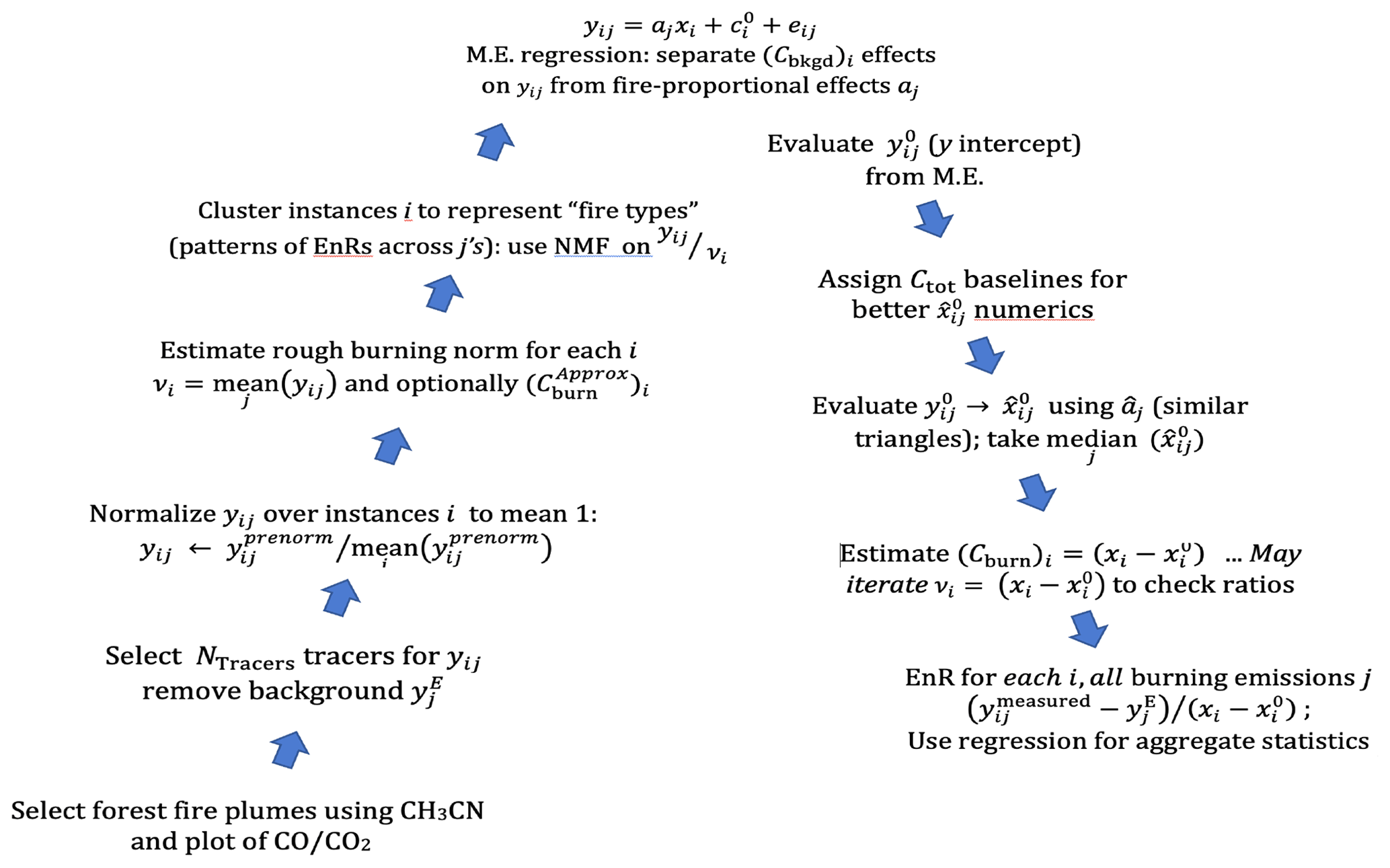
A summary of the MERET method as we currently propose it is shown in Fig. 8. It contains many steps, due to the need to disentangle background (C_burn)_i effects from a_j effects related to instance-by-instance EnRs and the variation in ${\widehat{a}}_j$ by fire type.

Figure 8 Summary of the MERET algorithm. See text for further detail.

1. Select a dataset of likeliest forest fire emission plumes, where CH₃CN > 0.125 ppt (clear biomass-burning signal) and excluding urban influence $\left(\mathrm{CO}-{\mathrm{CO}}^{\mathrm{Env}}\right)/\left({\mathrm{CO}}_{\mathrm{2}}-{{\mathrm{CO}}_{\mathrm{2}}}^{\mathrm{Backg}}\right)$ > 33 $\times {\mathrm{10}}^{-\mathrm{3}}$.

2. Select N_Tracer > 3 fire tracers with estimable environmental background values of $y_j^{\mathrm{E}}$ and subtract from plume instances. Nearby values sufficiently distant from plumes provide a good guide unless the tracer has very strong nonfire sources (e.g., CH₄ in California valleys). $y_{ij}^{\text{prenormalized}}\leftarrow \left(y_{ij}^{\mathrm{measured}}-y_j^{\mathrm{E}}\right)$.

3. Normalize the tracers above backgrounds: $y_{ij}=y_{ij}^{\text{prenormalized}}/\underset{i}{\mathrm{mean}}\left(y_{ij}^{\text{prenormalized}}\right)$.

4. Create values ratioed to a general fire-influence parameter: ${\mathit{\nu }}_i=\underset{j}{\mathrm{mean}}\left(y_{ij}\right)$. Create y_ij∕ν_i. Preliminary ${\left(C_{\mathrm{burn}}^{\mathrm{Approx}}\right)}_i$ may be estimated based on ν_i, for reference.

5. Roughly cluster plumes into N_Types clusters using ratioed values of y_ij∕ν_i to estimate fire types corresponding to varying EnRs common to species j. The value of N_Types was observed to make little difference. We used N_Types=6. Allow j to signify tracers within clusters.

6. Use mixed-effects regression to make estimates of intercepts and slopes ${\widehat{y}}_{ij}^{\mathrm{0}}$ and ${\widehat{a}}_j$ using a mixed-effects regression like main.lmer, allowing random effects corresponding to species (or species and type of fire) and by instance. Regress $y_{ij}=a_j{x}_i+c_i^{\mathrm{0}}+e_{ij}$, and estimate the fitted values of ${\widehat{y}}_{ij}$.

7. Prepare to estimate ${\widehat{x}}_{ij}^{\mathrm{0}}$. For numerical reasons, select an offset to apply to plumes that follows lower plume values, approximately 2 ppm less. Better discrimination makes for tighter estimates of ${\widehat{x}}_{ij}^{\mathrm{0}}$ in the next step.

8. Calculate ${\widehat{x}}_{ij}^{\mathrm{0}}=\left({\widehat{y}}_{ij}-y_{ij}^{\mathrm{0}}\right)/{\widehat{a}}_j$ from the fitted ${\widehat{y}}_{ij}$ values: take ${\widehat{x}}_i^{\mathrm{0}}=\underset{j}{\mathrm{median}}{\widehat{x}}_{ij}^{\mathrm{0}}$. Medians are little affected by exact choices in item 7, but spreads of estimates are affected.

9. Estimate $(C_{\mathrm{burn}}{)}_i=\left(x_i-{\widehat{x}}_i^{\mathrm{0}}\right)$. The results for equivalent-background ${\widehat{x}}_i^{\mathrm{0}}$ and C_burn are shown in Fig. 9 and are discussed more in Sect. 7. EnRs may now be calculated using Eq. (20). One may also use (C_burn)_i recursively, returning to steps 4–9 until convergence. However, for our dataset this made an inconsequential difference.

10. Use $\left(x_i-{\widehat{x}}_{ij}^{\mathrm{0}}\right)$ to estimate EnRs for any fire emission including tracers, using EnR for each i and $j=\left(y_{ij}^{\mathrm{measured}}-y_j^{\mathrm{E}}\right)/\left(x_i-x_i^{\mathrm{0}}\right)$; evaluate EnR to estimate ER and EF, considering possible transformation from the emission to measurement point.

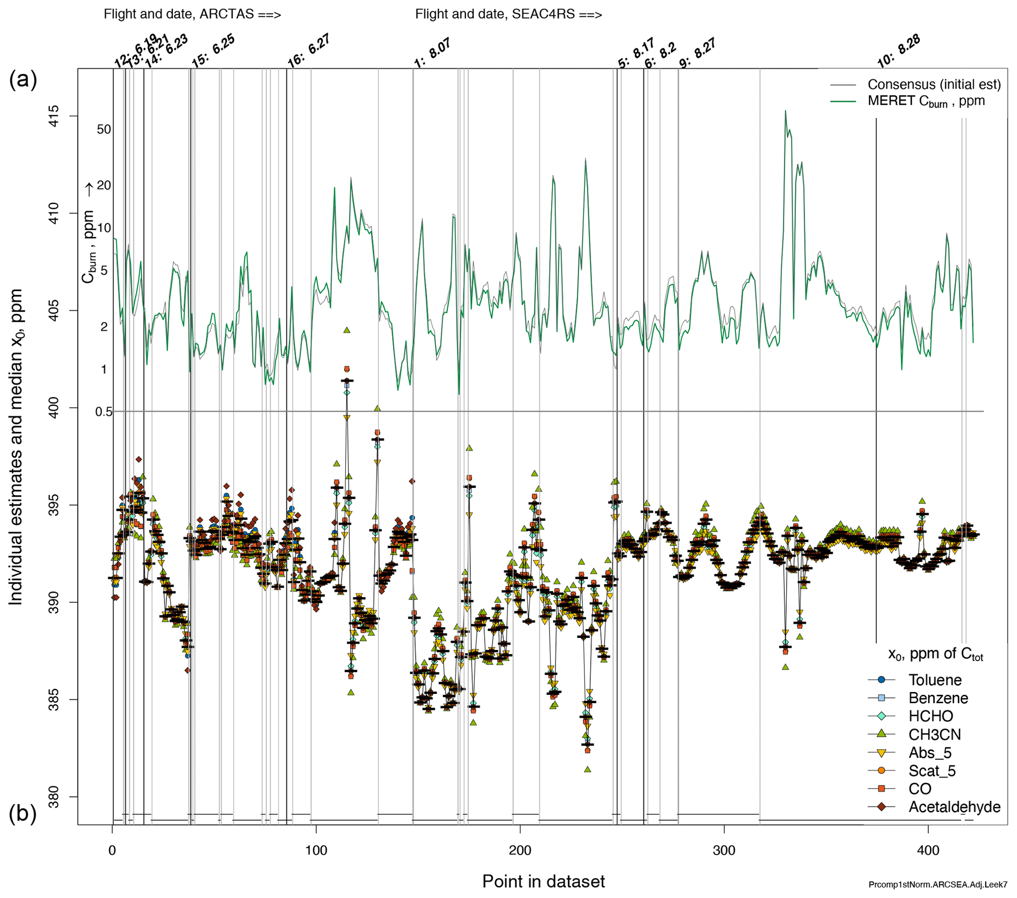
Figure 9 (b) Estimates of the 422 background ${\widehat{x}}_i^{\mathrm{0}}={\mathrm{CO}}_{\mathrm{2}}+\mathrm{CO}$ concentrations implied based on the eight fire tracers indicated in the legend. Contributing individual estimates ${\widehat{x}}_{ij}^{\mathrm{0}}$ are shown by overlapping colored points, with the median estimate ${\widehat{x}}_i^{\mathrm{0}}$ indicated by a black bar. Usually the colored points overlap closely; this indicates strong agreement. (a) Estimates of $C_{\mathrm{burn}}=x_i-{\widehat{x}}_i^{\mathrm{0}}$ indicators of fuel carbon burned, in the thick green line. The preliminary estimate of C_burn based on the consensus of tracer deviations (without variable EnR estimates) is also shown in a thin line. A scale factor, maximizing overlap with the thick line, was necessarily estimated by regression. Flight days are indicated by the days marked on the top axes, and individual plumes, separated by nonplume concentrations of longer than 10 min, are shown as vertical separator lines. A set of horizontal lines at ∼ 400 ppm indicate selected intervals for optimizing numerics (see text, Sect. 6.3, item 7).

More technical observations are these:

• a.

  For the use of an offset in calculations, we subtracted a baseline, C_baseline, a value determined as a constant for contiguous intervals, shown later in Sect. 7 and Fig. 9, and yielding a ∼ 2 ppm offset. We found that this minimized skewness and variance in the ${\widehat{x}}_{ij}^{\mathrm{0}}$ estimates for each observation instance i. It is comforting that the effect of differing offsets on the values of the median, $x_i^{\mathrm{0}}$, is small, < 1 ppm. (Add the offset back into the C_baseline when reporting $x_i^{\mathrm{0}}$.)

• b.

  Note that sharp positive and negative excursions of $x_i^{\mathrm{0}}$ are seen near dramatic spikes in x_i. However, $\left(x_i-x_i^{\mathrm{0}}\right)$ and consequently the EnRs are little affected. We can only speculate that small differences in the time averaging of CO₂ and the tracers due to the instruments may explain these. Note also that the number of parameters $N_{\mathrm{Tracer}}\cdot N_{\mathrm{Types}}+N_{\mathrm{Instance}}$ for the mixed-effects regression remains ≪ N_Tracer⋅N_Instance so that the mixed-effects regression is very strongly determined.

• c.

  The number of classes allowed in step 5 matters little over two or three. Adding additional classes (clusters) tends to add only minor variations in the slopes ${\widehat{a}}_j$. We are aware that overfitting effects can occur with many regression terms with positive and negative terms which mainly allow fitting of special cases. Here, harmful effects seen in overfitting of regression models are largely avoided by a requirement that the ${\widehat{a}}_j$ values be positive.

• d.

  As noted, it is possible to use this method recursively, making presumably better classifications of fire types. In our experience, while it is possible to make convergent, recursive characterizations of the C_burn quantity, tighter clustering, and more precise mixed-model lmer() estimates, the quantities $x_i^{\mathrm{0}}$ and $\left(x_i-x_i^{\mathrm{0}}\right)$ were just significant enough to warrant such care. If we had fewer than eight tracers available, such recursion might be important. We will incrementally update documentation of the code (Chatfield, 2020). New applications of the code will suggest improvements.

Here we outline a check on the consistency of C_burn estimation. The results for C_burn and tracer EnRs suggested to us that one likely source of uncertainty is that C_burn, ${\widehat{x}}_i^{\mathrm{0}}$, and the tracers may change very rapidly in comparison to our 1 min sampling intervals. Looking into this, we found that many of the C_burn estimates are of small magnitude; 12 of the 422 samples yielded C_burn < 1.5 ppm. Even large jumps from sample to sample in estimated ${\widehat{x}}_i^{\mathrm{0}}$ were not particularly associated with anomalous estimates of C_burn. The remaining, appealing possibility is occasional imprecise time alignment of all measurements, particularly of the CO₂ measurements. Such imprecise alignment could happen at any stage, from sampling line delays to interpolation to 1 min time intervals. Such variations in CO₂ would affect the ${\widehat{x}}_{ij}^{\mathrm{0}}$ found for all tracers in a coordinated way, just as was observed. Note that estimates of C_burn were little affected, since significant ${\widehat{x}}_{ij}^{\mathrm{0}}$ excursions were associated with large CO₂ + CO values. See Supplement, “Note on Examples of Enhancement Ratios”.

6.4 Number of independent samples

A natural broader question is, how well do these mean EnRs for a species represent the EnRs that might be measured in a large suite of significant forest fires in the Western USA? Clearly, this question can only be asked in the context of the sample provided by the two campaigns. Instances when the aircraft continued to sample smoke for many minutes could contain several types of plumes, as we will see illustrated for the Rim Fire plume of August 2013. The use of 10 s averages (if available) would not provide 6 times as much information about fire plumes as 60 s averages over the same measurement run. We tried a simple, approximate quantification of “independent instances” available to us using a frequently used formulation by Trenberth (1984). This can also be seen as providing one answer to the question, how many effectively independent samples of C_burn are there contributing to a mean, standard deviation, etc., of C_burn or the emissions factors for species, e.g., the CO tracer? That could be useful if instruments appeared to give imprecise measurements that required averaging. Trenberth assessed the correlation of successive observations by estimating an autoregressive AR(1) (i.e., Markov chain) model for a random variable ξ_i with parameter ϕ and random error ε_i, i.e., estimate of ${\mathit{\xi }}_{i+\mathrm{1}}=\mathit{\varphi }{\mathit{\xi }}_i+{\mathit{\epsilon }}_i$. We applied this for ${\mathit{\xi }}_i=x_i-x^{\mathrm{0}}$ (=C_burn) and several fire tracers y_ij, like toluene. Most contiguous sampling periods suggested around 0.6; this suggested Trenberth's “effective time between independent observations” as $\approx (\mathrm{1}+\mathit{\varphi })/(\mathrm{1}-\mathit{\varphi })$, about 4 min. For the DC-8, 4 min corresponds to about 15 km at lower-tropospheric airspeeds. The effect of this on the formal standard errors as described by a normal distribution was to increase them by a factor of ∼ 2. Roughly similar effects are expected for the empirical descriptions of EnR variability described below. Undoubtedly, for plumes within minutes of the source, the number of degrees of freedom corresponds more closely to the number of 1 min observations, but the number of such samples is low.

Not surprisingly, residuals in regressions of CO against C_burn are very little correlated. We surmise that such low correlation gives confidence in the mathematical determination of the mean regression slope. However, it does not provide help in answering the larger question, that of relevance in new situations. The sequential samples of plumes may have features like nonstationarity and selection bias; we hope that these ideas suggest more sophisticated analyses of relevance, left to future work.

7 Results – estimation of $x_i^{\mathrm{0}}$ and C_burn

The important results of the mixed model are the background ${\widehat{x}}_i^{\mathrm{0}}$ and even more importantly the incremental carbon liberated to the atmosphere, $C_{\mathrm{burn}}=x_i-{\widehat{x}}_i^{\mathrm{0}}$. The background estimates of ${\widehat{x}}_i^{\mathrm{0}}$ for all samples and the contributing individual estimates ${\widehat{x}}_{ij}^{\mathrm{0}}$ are shown in Fig. 9. The median ${\widehat{x}}_i^{\mathrm{0}}$ is shown as a thin black line. The colored circles in the legend identify how the tracer species j contribute an individual ${\widehat{x}}_{ij}^{\mathrm{0}}$ value, determining the median ${\widehat{x}}_{ij}^{\mathrm{0}}$.

What are the uncertainties in the estimates we have made of ${\widehat{x}}_i^{\mathrm{0}}$ and C_burn? The uncertainty in estimated carbon burned $\left(x_i-{\widehat{x}}_i^{\mathrm{0}}\right)$ plays an important role in the ultimate estimates, the emission factors. In this section, we will confine our exposition to this uncertainty for now. The graphs of ${\widehat{x}}_i^{\mathrm{0}}$ and $\left(x_i-{\widehat{x}}_i^{\mathrm{0}}\right)$ shown in Fig. 9 provide a practical understanding of the uncertainty. Note the continuity in ${\widehat{x}}_i^{\mathrm{0}}$; this important observation is described below. Traditional estimation of uncertainties for $\left(x_i-{\widehat{x}}_i^{\mathrm{0}}\right)$ is complex due to the several steps involved and the use of median estimates. The advisability of using the median estimator and its statistical properties have long been recognized (Laplace, 1774; Lawrence, 2013). This variety of uncertainty estimation may be useful as MERET is refined. However, we expect that the study of uncertainty depends more on evaluating sources of true variability in the EnRs and also on the conservation of tracer concentrations from the flames to the sampling point than on the mathematics of median estimation. Consequently, the following paragraphs explore these questions related to the number and choice of tracers. We suggest that the typical strong overlap of the individual-tracer values may reflect the high precision of the observer's techniques!

How does the number of tracers affect results? What are the effects of using alternate or simpler sets of tracers? How many tracers are required for stable estimates? We began to address these questions by examining estimates made with fewer tracers in the intercept-determining set: the selection of the set of j values. The Supplement gives two examples of subsets (“Note on Sensitivity to Number of Tracers Used”). Here is a summary of that material. The two sets chosen are those that are the most unambiguous indicators of ${\widehat{x}}_{ij}^{\mathrm{0}}$ based on their mutual agreement with ${\widehat{x}}_i^{\mathrm{0}}$ from the full set of 10 tracers. They are Set 1 (CO, Scat_5, and HCHO) and Set 2 (CO, Scat_5, HCHO, acetaldehyde, and toluene). These are indicated by an examination of Fig. S2 in the Supplement. (Abs_5 contributed ${\widehat{x}}_{ij}^{\mathrm{0}}$, which is the most deviating estimate from ${\widehat{x}}_{ij}^{\mathrm{0}}$.) Set 2 gave variations around of 0.02 ppm; the smaller set, Set 1, gave very similar variations except for the flights of 22 and 25 June, where many observation instances varied by around 0.1 ppm but with 11 points out of 422 differing by 0.3 ppm. This level of agreement surprised us. More significantly for our aims, the relative error in C_burn was only about 2 %. When sets containing the less correlated tracers were used, deviations ranged up to 0.2–0.4 ppm, which still appeared remarkably small.

Observation-to-observation consistency in ${\widehat{x}}_i^{\mathrm{0}}$ estimates, seen for most plumes observed in Fig. 9, is the strongest argument for the precision of the C_burn estimates. Recall that our theory does not use sequential time information; thus, successive estimates are essentially independent of each other. There is of course the dependency due to each observation's contribution to the estimate as one component of the entire dataset. This continuity is maintained even though the magnitudes of CO₂ + CO and estimated C_burn can change dramatically as the sampling aircraft enters and leaves each plume. Smooth excursions seen early in the flight marked 8.27 are explicable in terms of large changes in sampling altitude and location around the Rim Fire on that day. There are variations in ${\widehat{x}}_i^{\mathrm{0}}$ from plume to plume and from day to day.

In contrast to this typical continuity of ${\widehat{x}}_i^{\mathrm{0}}$ estimates, there are 15 to 20 brief and large excursions which deserve some attention. Of course, these may be disregarded in obtaining a general picture of EnRs. All the tracers suggest these excursions of the median, although there is a larger variation between the individual-tracer-based estimates ${\widehat{x}}_{ij}^{\mathrm{0}}$. These excursions are always associated with large changes in CO₂ + CO and C_burn, but often they occur 1 min later. We examined these excursions in detail. They do not seem to relate to changes in the EnRs' ${\widehat{a}}_j$ (as qualified by fire type) estimated simultaneously. The observations y_ij and the fitted ${\widehat{y}}_{ij}$ agree well, as do the nonexcursion points. Note however, that we may only use a single set of fire types, independent of j, to construct a set of ${\widehat{a}}_j$ values and ${\widehat{y}}_{ij}$ to make the ${\widehat{x}}_{ij}^{\mathrm{0}}$ estimates.

The results for C_burn and tracer EnRs suggested to us that one likely source of uncertainty is that C_burn, ${\widehat{x}}_i^{\mathrm{0}}$, and the tracers may change very rapidly in comparison to our 1 min sampling intervals. This would seem to be a concern since some C_burn estimates are of a small magnitude: 12 of the 422 samples yielded C_burn < 1.5 ppm. However, large jumps from sample to sample in estimated ${\widehat{x}}_i^{\mathrm{0}}$ were not particularly associated with anomalous estimates of C_burn. The remaining, appealing possibility is occasional imprecise time alignment of all measurements, particularly of the CO₂ measurements. Such imprecise alignment could happen at any stage, from sampling line delays to interpolation to 1 min time intervals. Such variations in CO₂ would affect the ${\widehat{x}}_{ij}^{\mathrm{0}}$ found for all tracers in a coordinated way, just as was observed. Note that estimates of C_burn were little affected, since significant ${\widehat{x}}_{ij}^{\mathrm{0}}$ excursions were associated with large CO₂ + CO values.

MERET should work better with more tracers, since more fire types may be revealed. However, additional classes (clusters) tend to add only minor variations in the slopes ${\widehat{a}}_j$. Furthermore, harmful effects often seen in the overfitting of regression models should be minimized by a requirement that the ${\widehat{a}}_j$ values be positive. (Positive and negative regression coefficients that allow the fitting of just a few points cannot be added.)

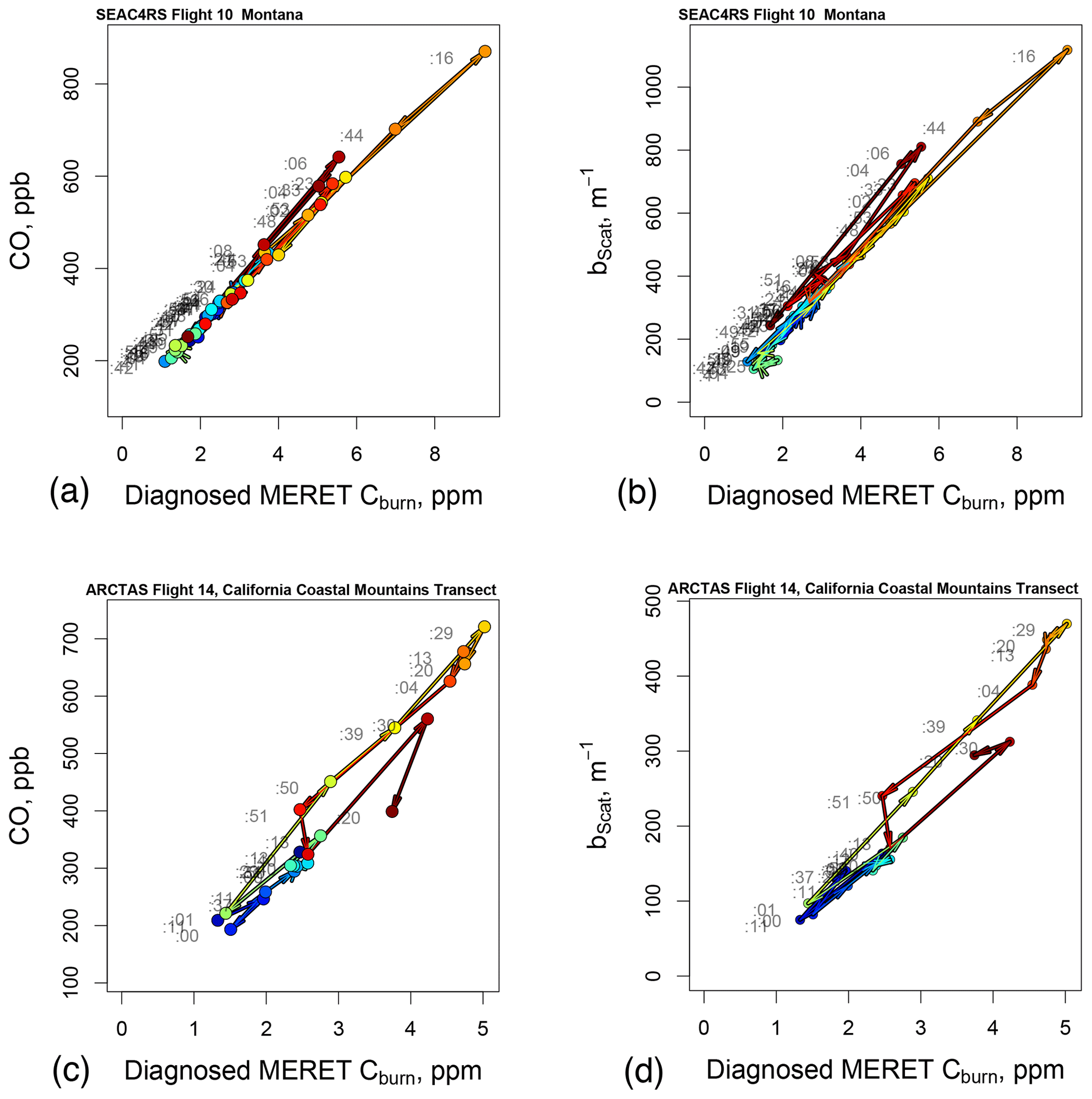
Figure 10 Analyzed relation of tracers to carbon burned using MERET for portions of SEAC4RS Flight 10 and ARCTAS Flight 14. Compare panels (a) through (d) with Fig. 4b, c, e, and f. Colors key the observations to times shown in the timelines in Fig. 4a and c. Light gray numerals give observation times in minutes.

8 Estimates of emission ratios – two MERET examples

8.1 MERET results for our two examples

The usefulness of our estimates of ${\widehat{x}}_i^{\mathrm{0}}$ and $C_{\mathrm{burn}}=x_i-{\widehat{x}}_i^{\mathrm{0}}$ is seen in the MERET analysis (Fig. 10) of the two case studies analyzed above using the NEMR approach, with portions of flights 10 and 14 shown in Fig. 4. The tracers CO and b_scat appear much better correlated with the C_burn estimated from MERET, especially in Flight 14. The plots for both CO and scattering imply linear relationships with an implied intercept near 0; i.e., background values of y_i have been satisfactorily removed. Difficulties with a variable C_bkgd appear to be resolved. However, the slopes of all the lines do not all agree. The Montana scatterplots (Fig. 4a) and (Fig. 4b) appear to suggest two slightly different linear features. The California transect scatterplots (Fig. 4c) and (Fig. 4d) show more separated linear features, though the slopes are parallel. We expect that these might correspond to varying fire types and perhaps varying MCEs, to be discussed in Chatfield and Andreae (2020), or to variations in background values of $y_j^{\mathrm{0}}$, which are much harder to detect with either MERET or the NEMR approach. A combined approach, using MERET to locate regions of similar MCE, might be useful here. Also, note that the variation in slope is more evident for b_scat than CO, emphasizing the special role of CO as the single best fire tracer, closely followed by b_scat.

Table 3 EnR estimates for fire emissions considered.

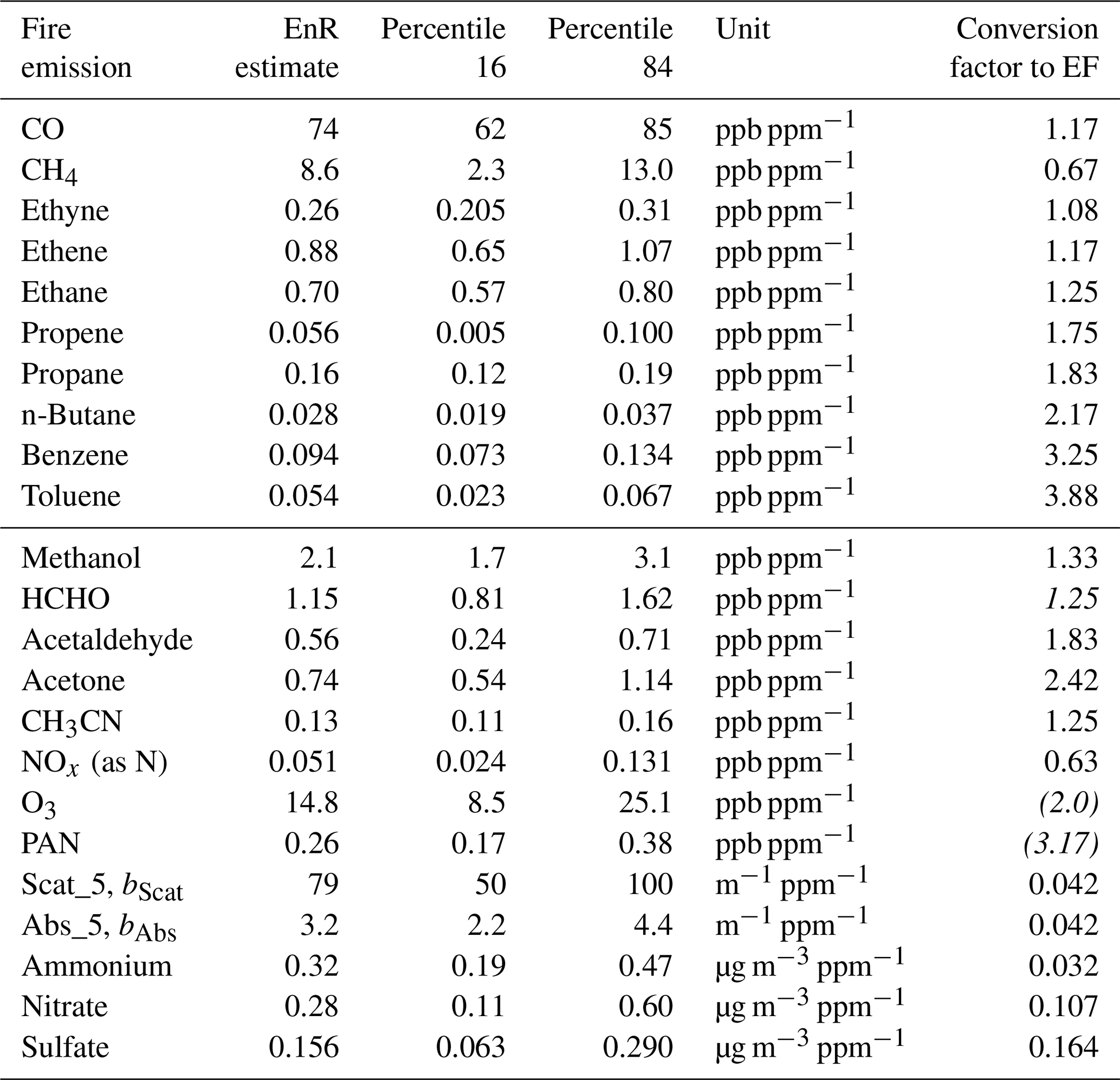
Notes: conversions assume a C to dry biomass ratio of 0.5. Conversions to micrograms per cubic meter assume a temperature of 25 ^∘C and atmospheric pressure of 1013 hPa. O₃ and PAN are not directly produced by fires. HCHO is produced but often decreases rapidly. Under appropriate conditions indicated in Chatfield and Andreae (2020), the EnR estimates can be used as ERs. For tracers that are rapidly removed or transformed, these tend to be the higher values. Parentheses in the last column indicate that the entry is an emission relationship, not EF, as O₃ and PAN are not directly emitted.

8.2 Table of several significant emissions

Table 3 provides a summary of the EnR relationships for some of the most significant gaseous emissions and particulate properties. In many cases, these EnRs can be converted to ERs and emission factors when the relationship of airborne C_burn to surface fuel consumed can be established. For the most highly reactive species, these EnRs will tend to be underestimates. An interpretive paper (Chatfield and Andreae, 2020) will give additional information on the photochemical age of the observation in many cases. Ozone and peroxy acetyl nitrate (PAN) are not emissions but produced in the plumes. Their relationships to fuel burned and their variations are nevertheless interesting. Descriptions of variation are given as the 16th and 84th percentiles of all the estimates. These are similar to error estimates if nothing more is known about the origin and age of the particular samples, a matter more fully discussed in Chatfield and Andreae (2020). EnRs as they varied in time and in relationship to measures of photochemical processing are shown in the Supplement, “Note on Examples of Enhancement Ratios”.

9 Conclusions

A major problem with the estimation of fire enhancement ratios and emission factors is inherent in their character: flames promote mixing in their plumes. Total carbon liberated to the atmosphere (approximately $C_{\mathrm{burn}}={\mathrm{CO}}_{\mathrm{2}}+\mathrm{CO}$) is mixed with background air at different points in the plume's evolution, and removal of that mixing effect has been a difficulty. The NEMR technique often uses CO as a unique tracer, but the EnR of CO is variable, adding uncertainty to the estimation of the EFs. Given the variability of CO due to combustion efficiency (MCE) and environmental variability, it has been emphasized that the NEMR technique can only be confidently applied in situations in which conditions affecting the ratio of CO to (CO₂ + CO) can be well determined, ideally from source to sampling (Yokelson et al., 2013). The method also tends to emphasize the use of samples of CO and tracer collected over many minutes so that the regression method for EnRs of tracer relative to CO, defining $a_{\mathrm{CO}\leftarrow \left(\text{fire-added}{C}_{\mathrm{burn}}\right)}$, becomes stable and a conversion to fuel carbon burned becomes possible.

We sought to decompose C_tot into C_bkgd and C_burn. However, meteorology and mixing allow significant variations in C_bkgd due to other powerful processes, e.g., CO₂ from respiration and photosynthesis in mixed-layer air. Once lofted, C_bkgd varies little unless the plume enters layers of free tropospheric air from long-range transport with different C_bkgd values, which further dilute the plume (Yokelson et al., 2013). We noted such problems using the NEMR method in analyzing a significant number of plumes for enhancement ratios studied in the Western USA during two campaigns, ARCTAS California and SEAC4RS, with 1 min samples totalling 422 in all.

The problem of deriving an accurate C_bkgd is solved by noticing that there are two different kinds of information provided by multiple observational instances of a tracer and multiple tracers at a single instance. Information about the various EnRs and C_bkgd values is mixed but not inextricably. There is a solution based on mixed-effects (also called random-effects) regression modeling. We propose a mixed-effects regression emission technique (MERET) to replace or at least to check on the NEMR approach, for which we used the R routine lmer().

MERET is related to traditional entraining-plume models for parcels. We presented a synthesis describing multiple tracers from fire to sampling location. Sample calculations with the model suggest that it deals linearly with several varied histories for plume mixing. This motivates a regression equation for an equivalent-background $x_i^{\mathrm{0}}$ value for each observation that is related to entraining concentrations x^E(t) along the trajectory and shows coherent agreement for each tracer species (Fig. 9). The theory then allows this $x_i^{\mathrm{0}}$ to be used to define C_burn and thus to define the EnR for any appropriate fire-derived variable. This technique should allow EnRs in more variable, difficult situations and allows estimates of EnRs for individual samples.

EnRs are useful for the estimation of emission factors when the plume age is short compared to the transformation timescale of the measured fire tracer, and we provide an approximate diagnostic for this age for most samples. Formaldehyde, acetaldehyde, the alkenes, benzene, NO_x, b_Scat, and b_Abs particularly require such attention.

Carbon monoxide is usually the best single tracer that correlates with fire emissions (C_burn), supporting the use of the NEMR technique. Our analysis suggests other tracers had EnR variations that collectively helped to distinguish C_burn from CO in regression. The NEMR methodology depends on a full analysis of the history of CO influences on a sample to obtain a reliable MCE. MERET allows estimates of MCE as well as of C_burn for each sample. Thus it demarcates sampling periods with nearly homogeneous MCE. However, possible large variations in the entraining background of CO should still be considered carefully in dilute plumes with C_burn < 2 ppm.

Questions for future research

We conclude with some questions for future research; these also review the suggested conclusions of this paper and acknowledge the limitations of a single publication.

1. How well can the use of one or a few tracers, e.g., CO, b_scat, and HCHO, actually constrain EnRs and EFs when only a few instruments may be used? How many variables need to be measured or how fresh should the plumes be to allow CO to be used both as a fire tracer and to allow useful estimates of MCE?

2. Can MERET be used to identify time periods of relatively homogeneous MCE, and can that MCE value be used with the NEMR to create suitable EnRs? Since the NEMR uses differences sample by sample (in time), no minimum value of another tracer needs to be estimated. (Consider that MERET does allow some evaluation of the minimum value estimate to be assessed and a better minimum assigned.)

3. Can MERET, the NEMR, and better near-fire nonplume sampling help us to prevent misattribution of fire emissions? These would include observations for fire intake air, air likely to be entrained in ascent, and air surrounding a plume and likely to be entrained as a plume spreads downwind. Can simulations of entraining plumes aid this effort?

4. What do fire types represent, and which species or properties tend to correlate in their EnRs (Chatfield and Andreae, 2020)?