the Creative Commons Attribution 4.0 License.
the Creative Commons Attribution 4.0 License.
 | 02 Mar 2020
Comparison of turbulence measurements by a CSAT3B sonic anemometer and a high-resolution bistatic Doppler lidar
Michael Eggert
Christian Gutsmuths
Stefan Oertel
Paul Wilhelm
Ingo Voelksch
Luise Wanner
Jens Tambke
Ivan Bogoev
Accurate measurements of turbulence statistics in the atmosphere are important for eddy-covariance measurements, wind energy research, and the validation of atmospheric numerical models. Sonic anemometers are widely used for these applications. However, these instruments are prone to probe-induced flow distortion effects, and the magnitude of the resulting errors has been debated due to the lack of an absolute reference instrument under field conditions. Here, we present the results of an intercomparison experiment between a CSAT3B sonic anemometer and a high-resolution bistatic Doppler lidar, which is inherently free of any flow distortion. This novel remote sensing instrument has otherwise very similar spatial and temporal sampling characteristics to the sonic anemometer and hence served as a reference for this comparison. The presented measurements were carried out over flat homogeneous terrain at a measurement height of 30 m. We provide a comparative statistical analysis of the resulting mean wind velocities, the standard deviations of the vertical wind speed and the friction velocity and investigate the reasons for the observed deviations based on the turbulence spectra and co-spectra. Our results show an agreement of the mean wind velocity measurements and the standard deviations of the vertical wind speed with a comparability of 0.082 and 0.020 m s−1, respectively. Biases for these two quantities were 0.003 and 0.012 m s−1, respectively. Slightly larger differences were observed for friction velocity. Analysis of the corresponding co-spectra showed that the CSAT3B underestimates this quantity systematically by about 3 % on average as a result of co-spectral losses in the frequency range between 0.1 and 5 s−1. We also found that an angle-of-attack-dependent transducer-shadowing correction does not improve the agreement between the CSAT3B and the Physikalisch-Technische Bundesanstalt (PTB) lidar effectively.
- Article
(9257 KB) - Full-text XML
- BibTeX
- EndNote


Accurate fast-response measurements of the three-dimensional wind vector are of great importance to fundamental research in micrometeorology for flux measurements using the eddy-covariance methods in ecological studies (Aubinet et al., 2012). However, in recent years, several studies found that most, if not all, sonic anemometers may be afflicted by a systematic underestimation of turbulent fluctuations due to probe-induced flow distortion errors (Frank et al., 2013, 2016; Wyngaard, 1988). These errors can be further classified into errors due to transducer self-shadowing caused by cross-shadowing and influences of the support structure. This has been demonstrated in field studies by means of specially modified reference instruments with a vertical measurement path, so that the measurement path is perfectly perpendicular to the horizontal flow, or by rotating an additional sonic anemometer 90∘ around the x axis for comparison. An intercomparison experiment between six different commercially available sonic anemometers showed that all participating instruments agreed very well (Mauder and Zeeman, 2018). Nevertheless, it is possible that all instruments measure vertical fluxes with similar inaccuracies, since no independent reference measurement was available. Consequently, the absolute magnitude of the potential bias remains unknown.
A particular sonic anemometer, the CSAT3 (Campbell Scientific Inc., Logan, Utah, USA) and its variant the CSAT3B, have been investigated intensively. It is one of the most widely used and highly reputed instruments, which has often served as a reference in past intercomparison studies (Foken and Oncley, 1995; Loescher et al., 2005; Mauder et al., 2007). Features such as its small transducer diameter, 30∘ tilt angle with respect to the vertical axis, short sonic path length, and symmetrical boom design, following the recommendations of Wyngaard (1988), increase confidence in its high-fidelity vertical wind fluctuation measurements. Based on the results of a field comparison with an orthogonal sonic anemometer as reference, Horst et al. (2015, hereafter H15) propose a wind-tunnel-derived correction for the CSAT3, which typically leads to an increase in vertical wind fluctuations and hence also vertical fluxes by 4 % to 5 %.
A numerical simulation of the flow around this instrument indicates that the H15 correction actually reduced the measurement error of common turbulence statistics, but a considerable uncertainty remained (Huq et al., 2017). This study found that the error is dependent on the azimuth angle, which can be explained by cross-shadowing effects. A similar wind direction dependence of the CSAT3's flow distortion error was also found in a field experiment in comparison to another non-orthogonal sonic anemometer (Grare et al., 2016). Moreover, a spectral analysis based on theoretically derived ratios between the different wind components in the inertial subrange substantiates the earlier finding that the correction by H15 only partially compensates for the CSAT3's flow distortion error (Peña et al., 2019). Nevertheless, the main problem of all these past investigations has been the lack of an accurate standard reference for the measurement of turbulent flow statistics, since wind tunnel calibrations of sonic anemometers are conducted under quasi-laminar conditions at much lower Reynolds numbers than in the free atmosphere and therefore their transferability to measurements in the field is questionable (Högström and Smedman, 2004). Further problems of past studies are the influence of shadowing between adjacent sensors and support structures, and lack of homogenous flat terrain. Our study seeks to overcome the limitations and uncertainties of previous experiments comparing sonic anemometers in the field.
As a reference instrument, we employ a high-resolution bistatic Doppler lidar, which has been developed at the Physikalisch-Technische Bundesanstalt (PTB) in Braunschweig, Germany (Oertel et al., 2019). This optical remote sensing device is naturally free of any flow distortion errors and determines the 3D wind vector in a volume of less than 0.0005 m3, for measurement heights up to 200 m at an output frequency of up to 10 s−1, which is comparable to the sampling characteristics of a typical sonic anemometer. The very small sampling volume of this lidar system has the advantage that both data sets can be directly compared, without the need for extensive modelling of spatial averaging effects, which would lead to a large uncertainty of the resulting turbulence statistics (Brugger et al., 2016). Hence, our objectives for this study are as follows:
-
comparing the measurement of turbulence statistics of a CSAT3B sonic anemometer with the PTB lidar during a side-by-side field deployment,
-
investigating reasons for the observed deviations by means of (co-)spectral analysis,
-
evaluating the correction proposed by H15 using the PTB lidar as a reference.
In this analysis, we will mainly focus on three statistics: (i) the mean wind velocity, as this quantity is of high relevance for a number of applications, especially in wind energy research; (ii) the standard deviation of the vertical velocity component, as errors in this variable directly translate into errors of fluxes between ecosystems and the atmosphere when using the eddy-covariance method; and (iii) friction velocity, as this quantity is crucial for the validation of meteorological models (Tambke et al., 2005). To better understand the reasons for the differences between both instruments, we will analyse spectra and co-spectra of the observed turbulent time series, including an analysis of spectral ratios of wind components in the inertial subrange as proposed by Peña et al. (2019).
2.1 Instruments
2.1.1 CSAT3B sonic anemometer
The CSAT3B sonic anemometer used in this study is the successor of the well-established CSAT3. The biggest difference to the CSAT3 is an improved placement of the control electronics inside the mounting block of the sensor head, whereas the sensor geometry, the measurement principle, etc., remained the same, so that findings of previous studies conducted with the CSAT3 are transferable to this study. The sensor geometry of the CSAT3B follows Zhang et al. (1986) and is optimized for low flow distortion due to transducer wakes designed for predominantly horizontal flow. In comparison to previous sonic anemometers with orthogonal sonic paths, where the horizontal velocity components are measured from a pair of axes located in the horizontal plane and the vertical velocity is measured by a single vertical pair of transducers, the flow distortion effects in the CSAT3B are reduced by positioning all six transducers and their supporting structures out of the horizontal plane. This is important because horizontal wind velocities are usually much larger than vertical wind velocities, and when using sonic anemometers with non-orthogonal paths a distorted measurement of the horizontal wind speed directly affects the vertical wind speed measurement. Each sonic path is tilted 30∘ from the vertical axis and spaced 120∘ apart in the horizontal plane. The length of the sonic path is 0.1154 m and the diameter of the ultrasonic transducers is 0.00635 m, giving a path length to diameter ratio of 18, which is larger than those of other commercially available instruments (Mauder and Zeeman, 2018). The higher this ratio and the steeper the angle between the sonic path and the vertical axis, the fewer self-shadowing effects are expected on the wind measurement because a smaller portion of the path is affected by the transducer wake (Kaimal, 1979; Wyngaard and Zhang, 1985).
As part of the calibration procedure, the sonic path length (the distance between the transducers) and the actual values of the angles of the sonic axes of each individual CSAT3B instrument are precisely determined with a coordinate measuring machine and stored in the internal non-volatile memory. The wind speed along each sonic path is calculated from the sonic path distance between each pair of transducers and the difference of the reciprocal of the times of flight (TOF) of the ultrasonic pulses travelling along the sonic axes in opposite directions. Accurate and precise TOF measurements are achieved using advanced digital processing techniques. The wind components along the three non-orthogonal sonic axes are transformed into orthogonal components using a 3×3 coordinate transformation matrix unique for each CSAT3B and derived from the actual angles determined during the geometry measurement procedure. To determine accurate TOF estimates and to account for ultrasonic transducer delays associated with the conversion of the electrical-to-acoustical signal, each CSAT3B is factory calibrated in a specially designed temperature-controlled zero-wind chamber over the entire operating temperature range of −30 to +50 ∘C. Any temperature-induced changes in the sonic path length are also compensated for during this procedure.
The speed of sound can also be measured by the CSAT3B using the measured transducer-to-transducer distance and sum of the reciprocal of the TOF of the pulses along the acoustic path travelling in opposite direction. The quality and accuracy of the CSAT3B acoustic temperature measurements are evaluated during calibration by comparison with an air temperature standard. This procedure provides additional independent verification of the fidelity of the TOF measurements and the accuracy of the sonic path distance.
2.1.2 Bistatic Doppler lidar
The most widely used wind remote sensing devices are conventional monostatic Doppler lidar systems that have been established in wind energy applications in recent years (e.g. Pearson et al., 2009). Such systems utilize a common transmitting and receiving beam that measures the wind velocity component in beam direction via a Doppler shift of the received scattering light from aerosols travelling along the path of the transmitting laser beam (Drain, 1980). To measure the complete wind vector, the common beam is tilted in different directions (Eder et al., 2015; Newman et al., 2016). Provided that the wind field is almost homogeneous within the measurement volume, these systems deliver reliable measurement results (Gottschall et al., 2012; Peña et al., 2009). However, leaving flat terrain and having to consider the inhomogeneous wind conditions that predominate over complex terrain, significant errors for the wind speed measured arise (Bradley, 2008) and can be on the order of 10 % (Bingöl et al., 2009). Thus, in the case of unidentified and complex wind fields, the reliability of monostatic lidar measurements becomes questionable without considering any other reference measurements.
The novel three-component lidar system developed by the PTB aims to overcome the present limitation to almost homogeneous wind fields given by the monostatic working principle (Oertel et al., 2019). The basic idea of this system relies on utilizing a bistatic measurement setup (Harris et al., 2001), i.e. on the use of one transmitting laser beam and three detection beams (spatial separation), in order to determine all three components of the wind vector simultaneously in a small measurement volume by means of the same aerosols (Fig. 1). In contrast to monostatic systems, which typically use a common transmitting and receiving unit and an optical circulator to separate the received scattering light, the bistatic system is based on one transmitter and three discrete, spatially separated receivers.
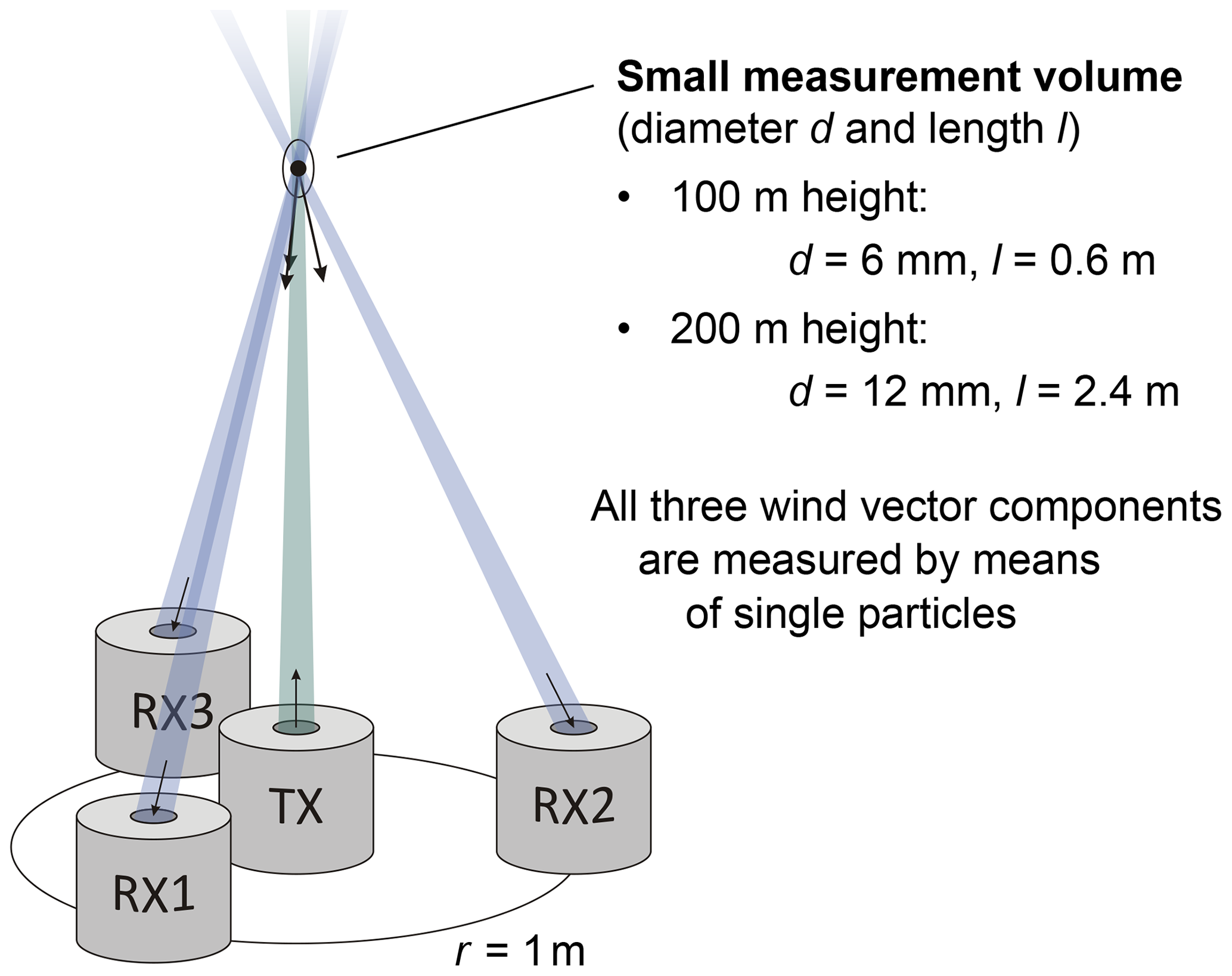
Figure 1Principle of the novel bistatic lidar consisting of one transmitting unit (TX) and three receiving units (RX).
The receivers are positioned at a radius of 1 m around the transmitter to ensure both sufficient particle-scattering light intensity (quasi-backward direction) and sufficient resolution for the determination of the horizontal velocity component. Each of the three heterodyne receivers converts the particle-scattering light of its respective receiving beam into an optical beat signal, which is then converted into an electrical signal by a differential photodetector. The measurement volume calculated according to Gaussian beam optics has a diameter of 2 mm and a length of 50 mm for a measurement height of 30 m above ground. A time-of-flight measurement of the overall optical path length is used to actively control the receiver optics in order to maintain the measurement volume at the desired well-known height. To ensure a mobile operation with stable working conditions in the field, especially with respect to requirements on the mechanical setup and the optoelectronics, the bistatic lidar system has been enclosed in a temperature-controlled housing unit mounted on a trailer (Fig. 2). The accuracy of the bistatic PTB lidar was validated with the laser Doppler anemometer (LDA) reference standard in a wind tunnel erected on a platform at a height of 8 m. Long-term measurements, each lasting 1 h, were carried out. At seven velocities between 4 and 16 m s−1 and different orientations of the lidar system, an average deviation of less than 0.4 % was observed.
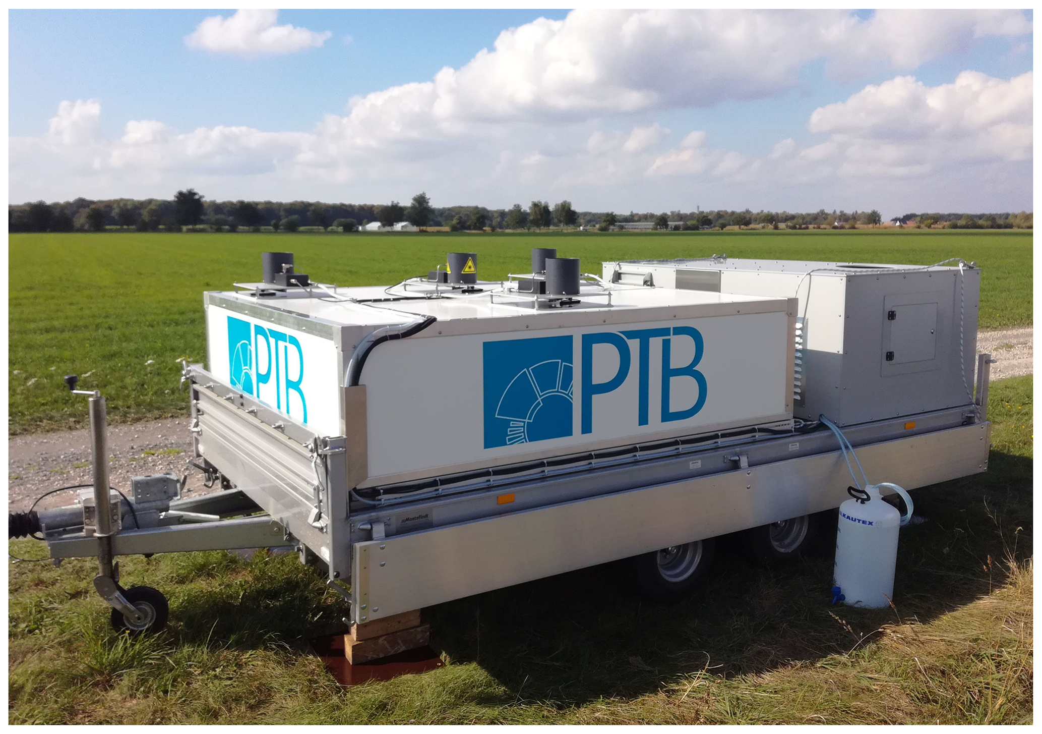
Figure 2Photograph of the bistatic PTB lidar at the measurement site (opened trailer housing).
2.2 Experimental setup
The field intercomparison experiment was set up at the boundary of a recently harvested maize field on the compound of the Johann Heinrich von Thünen-Institut in Braunschweig, Germany (52.2943∘ N, 10.4461∘ E, 81 ), and measurements were carried out from 09:00 UTC, 14 September 2018, until 06:00 UTC, 27 September 2018. The CSAT3B was installed on top of a trailer-mounted pneumatic telescopic mast (Clark Masts Systems Ltd., Binstead, UK) at a height of 30.5 m (Fig. 3). Its measuring volume was 0.85 m from the centre of the mast; the mast's diameter at mounting height was 0.05 m. Since the prevailing wind direction expected for the measurement period was west, the PTB lidar was set up approximately 9 m west of the trailer mast and the CSAT3B was oriented at 270∘. This setup was chosen, on the one hand, to minimize interference from the trailer mast with the PTB lidar measurements and interference from the anemometer's arms and the mast with the CSAT3B measurements on the other. Data acquisition from the CSAT3B was accomplished using a CR6 data logger (Campbell Scientific, Inc., Logan, Utah, USA) with SDM (Synchronous Device for Measurements) communications. The sampling rate was 10 s−1, and the three orthogonal (referenced to the anemometer head) wind components ux, uy, and uz (m s−1); the ultrasonic air temperature Ts (∘C); and the CSAT3B diagnostic flag were recorded. Measurement times were logged in UTC, and data acquisition systems were synchronized with a time server via the internet. The PTB lidar system recorded the measured (Doppler) frequency and amplitude of every detected scattered light signal. This raw data were also averaged to 10 s−1 velocity vectors afterwards.
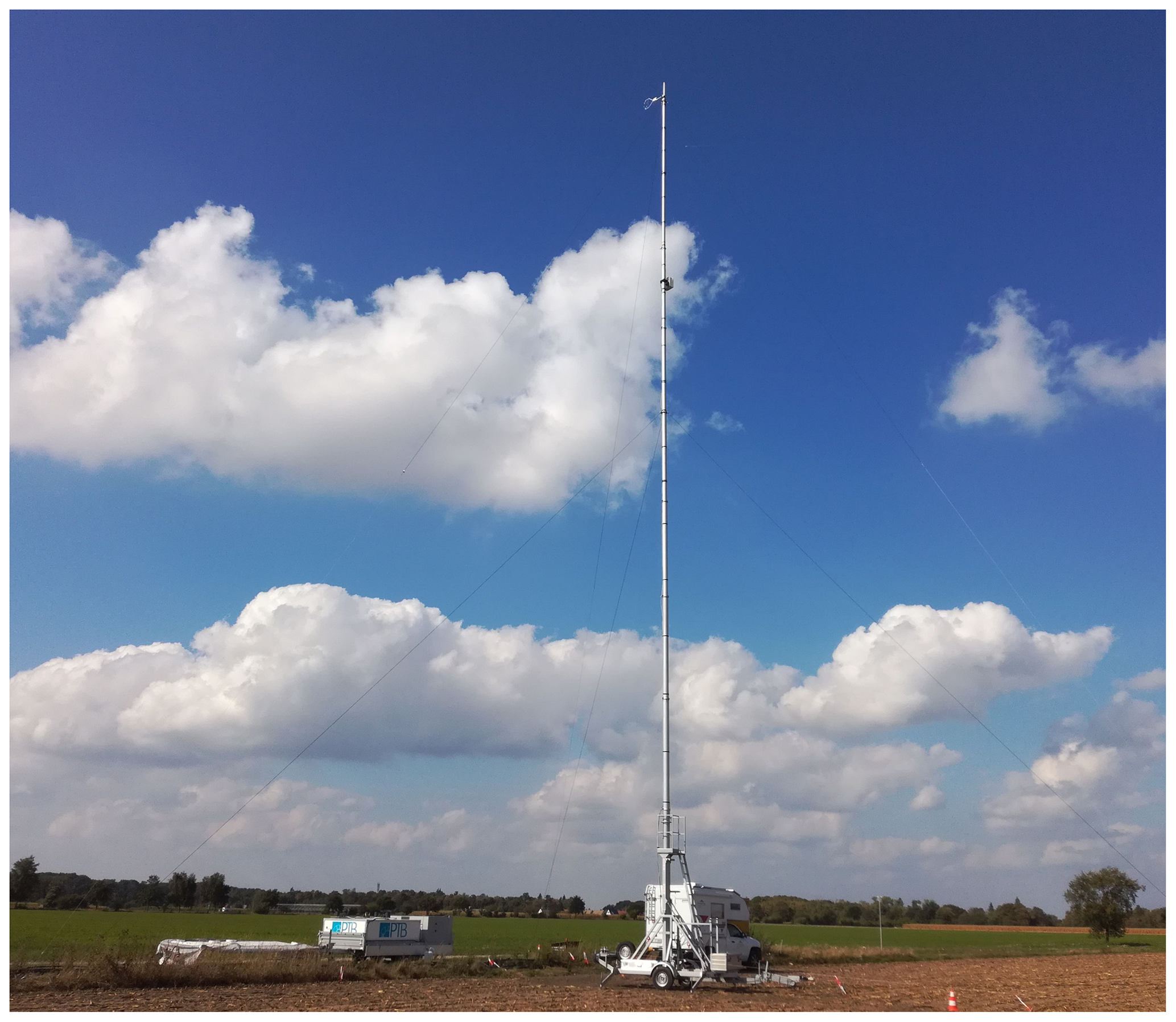
Figure 3Photograph of the setup of the field intercomparison experiment between the bistatic PTB lidar (left) and the CSAT3B mounted on a mobile 30 m telescopic mast (centre right). The camera is facing north-west.
2.3 Meteorological conditions
In a continuation of the previous months, the air temperature stayed relatively high for the first week of the measurement campaign, due to a series of high-pressure systems. The remains of an Atlantic hurricane (“Ex-Helene”) pushed hot air up to the northern border of Germany, which culminated in air temperatures of more than 30 ∘C on 18 September 2018 at the site of our experiment. The clear sky led to a strong diurnal variation in temperature with differences of up to 15 ∘C between the nocturnal minimum and the daytime maximum. The wind was relatively weak, with 10 min mean wind speeds (in 10 m height) ranging from 1 to 6 m s−1 and between 1 and 10 m s−1 for wind gusts. Wind speed was correlated with the variation in air temperature, with higher speeds at noon, due to more intense convection and better mixing, and lower speeds during the night. The wind direction was mostly between south and west. At noon on 21 September 2018, the air temperature dropped abruptly from more than 25 ∘C to less than 15 ∘C, accompanied by wind speeds of up to 11 m s−1, wind gusts of up to 20 m s−1, and some rain. During this second week, the nocturnal temperature minimum was 5 ∘C and wind speeds were generally higher than during the first week (Fig. 4).
2.4 Calculation of turbulence statistics
All turbulence statistics were calculated from the 10 s−1 raw data of both instruments using the eddy-covariance software TK3 (Mauder and Foken, 2015) with an averaging time of 30 min. The same settings were applied in TK3 for both data sets, including a spike detection algorithm (Mauder et al., 2013). In addition, we used the diagnostic flag of the CSAT3B for filtering of the raw data and screened our data for rain in the last hour, which may have affected the optics of the lidar and the transducers of the sonic anemometer. After this preparation of the raw data, we discarded any 30 min statistics if more than 10 % of the high-frequency data were missing, including those data rejected by the spike test. These are commonly used settings for eddy-covariance measurements (Fratini and Mauder, 2014; Mauder et al., 2013). For the CSAT3B, no spikes at all were detected for 92 % of the 618 30 min intervals, and for the PTB lidar, 73 % of the 618 30 min intervals were spike-free. This means application of the spike detection algorithm is important to ensure high data quality, but its impact on the comparison is limited. As a result of the data preparation described above, 615 30 min intervals remained for the CSAT3B and 458 remained for the PTB lidar. Subsequently, the raw turbulence statistics were corrected using the double rotation method (Kaimal and Finnigan, 1994), and a correction of low-pass filtering effects due to path length averaging (Moore, 1986) to allow for a direct comparison of both data sets. In an alternative processing stream, we applied the correction for transducer-shadowing effects by H15 in order to validate this method as part of this intercomparison experiment. To facilitate this, we implemented this method into the TK3 software based on a software script provided by Campbell Scientific Inc.
2.5 Statistical analysis of the comparison
For the statistical analysis of the intercomparison, an orthogonal Deming regression was applied in order to account for measurement errors in both x and y variables, using the R package mcr (Manuilova et al., 2014). In this regression analysis, we generally selected the PTB lidar data as the x variable and the sonic anemometer data as the y variable. In contrast to a traditional least-squares method, the orthogonal regression provides deviations measured perpendicularly and not parallel to the y axis, which addresses problems when there is a measurement error in both x and y variables and implies that errors in x and y have equal variances. Pearson's correlation coefficient r is also determined by using the same R package. Furthermore, we calculated comparability, which is equivalent to the root-mean-square error (RMSE), and bias, which is the mean error of a certain measurement quantity.
2.6 Spectral analysis
Based on dimensional analysis of energy distribution of turbulence, it has been deduced that spectra and co-spectra of fully developed turbulence follow similarity laws (Kolmogorov, 1941). Comparing the theoretically derived and measured spectra can be a powerful tool to investigate the performance of measuring instruments. Here, we focus on two spectral characteristics in the inertial subrange: (i) the ratio between the spectra of transversal wind velocity components, i.e. Svand Sw, and of the longitudinal component Su is theoretically derived to be 4∕3, and (ii) the power law behaviour with a slope of for spectra and for co-spectra (Kaimal and Finnigan, 1994). A ratio smaller than 4∕3 between Sw and Su indicates a general underestimation of vertical wind velocity or overestimation of the horizontal velocity (Peña et al., 2019). In case of high-frequency dampening, the slope of a measured spectrum drops below at the high-frequency end of the spectrum (Aubinet et al., 2000). This allows for the determination of the cut-off frequency fc, describing the associated sonic path averaging low-pass filter effect, by spectral analysis as proposed by, e.g. Ibrom et al. (2007). The half-hourly wind spectra are calculated using the TK3 software (Mauder and Foken, 2015), following the method of Stull (1988). Further processing is based on the method of Ibrom et al. (2007) for cut-off frequency determination. To investigate the ratio between Su, Sv, and Sw within the inertial subrange, the half-hourly spectra were weighted by frequency and exponentially binned. All u, v, and w spectra from 30 min intervals with absolute values of sensible heat flux larger than 10 W m−2 and absolute values of the stability parameter (z= measurement height; L= Obukhov length) were averaged to derive one ensemble spectrum. For the empirical determination of the cut-off frequency of the w measurements, half-hourly spectra Sw,norm were additionally normalized by the variance of w and inspected for blue noise.
We assume that the low-pass filtering of Sw,norm(f) can be described by the following function (Fratini et al., 2012),
where Fn is an additional normalization factor, which is intended to compensate for the reduction of the overall variance (Ibrom et al., 2007). We fitted the Sw,norm to Eq. (1) to determine the cut-off frequency, using the Levenberg–Marquardt non-linear least-squares algorithm as implemented in the R package minpack.lm (Elzhov et al., 2016). This fit was weighted by the number of frequencies in each bin. Instead of sonic temperature spectra, as proposed by Ibrom et al. (2007), we used the spectral models for vertical wind velocity Sw,mod(f) that are implemented in TK3 as universal reference spectra. These models are a corrected version of Moore (1986) for stable stratification and of Højstrup (1981) for unstable conditions. The model spectra were calculated for each 30 min interval and then averaged to one ensemble spectrum in order to determine the cut-off frequency. Please note that this does not apply to the ensemble spectra presented to determine the spectral ratios. These are purely based on measured spectra.
3.1 Comparison of turbulence statistics
Scatter plots and regression parameters for , , and u∗ generally show a good agreement between the CSAT3B and the PTB lidar measurements (Fig. 5, Table 1). Particularly, the measurements of the vertical velocity fluctuations are almost identical with a regression slope of 0.994, a correlation coefficient of 0.998, and a comparability of 0.017 m s−1. This is somewhat unexpected because previous studies indicated an underestimation of by 3 %–5 % due to probe-induced flow distortion (H15, Frank et al., 2016). However, only a very small negative bias of −0.009 m s−1 was found in our analysis using the flow-distortion-free PTB lidar as reference. One might argue that perhaps both instruments underestimated in the same way. However, we regard this as implausible because the measurement principles are very different and therefore it is unlikely that the effect of potential errors is so similar under this broad range of atmospheric conditions. Based on the remote optical measurement principle and the lack of any physical structure, it can safely be assumed that flow distortion errors can be ruled out for the lidar. Any potential high-frequency dampening effects of the lidar signal should be small considering its short measurement path of 0.05 m and the sampling frequency of 10 s−1. Furthermore, we have even compensated for those small low-pass filtering effects as part of the standard post-processing routine using the TK3 software (Moore, 1986).
Our findings partially contradict the conclusions of earlier sonic anemometer intercomparison studies that proposed vertical wind underestimation by the CSAT3 as the source of error on the order of 5 %. The discrepancy of our findings with the results from previous experiments can be explained by the lack of a suitable and accurate reference instrument. For example, H15 used an Applied Technologies, Inc. (ATI) K-probe sonic anemometer as a reference instrument, which they assumed to be more accurate because of its orthogonal transducer array. However, the measurements by this instrument are also corrected for flow distortion effects by a variable factor of 1.02, on average, for w measurements, and this wind-tunnel-based correction factor might not be applicable in the turbulent free atmosphere.

Figure 4Meteorological conditions during the intercomparison experiment based on 10 min data from the nearby weather station (ID 662, 52.2915∘ N, 10.4464∘ E, 81 ) of the German Weather Service (DWD). Data were provided by the DWD Climate Data Center (CDC).
Table 1Statistical quantities characterizing the differences between the measurements of the CSAT3B sonic anemometer and the PTB bistatic Doppler lidar, based on 458 paired observations of turbulence statistics, each averaged over 30 min. The statistics for the CSAT3B data after applying the H15 correction are shown in round brackets. The statistics without application of a low-pass filtering correction to either of the instruments are shown in square brackets ( is not altered).

The mean wind velocity also compares very well on average. There are just a few data points at higher wind speeds between 5 and 6 m s−1 for which the CSAT3B reports slightly larger values than the PTB lidar. Nevertheless, this comparison, with a very small bias of 0.003 m s−1 and a RMSE of 0.082 m s−1 (Table 1), is still as good as or even better than between two adjacent CSAT3 sonic anemometers (Mauder and Zeeman, 2018).
Friction velocity u∗ is typically more difficult to measure due to the spectral separation between the peaks in the u and w spectra. Nevertheless, the comparability of these values is still good between the two instruments, with an RMSE of 0.042 m s−1, which is again as good as between adjacent sonic anemometers (Mauder and Zeeman, 2018). However, the u∗ data measured by the CSAT3B are slightly too low compared to the PTB lidar, indicated by a regression slope of 0.973 and a bias of −0.009 m s−1 (Table 1). The differences in at larger wind speeds and the systematic differences in u∗ will be investigated further below.
As a first step, we assess whether the comparison of the CSAT3B data improves through application of the H15 method, which is intended to correct for flow distortion by transducer shadowing. However, as can be seen from Table 1, and show slightly larger differences from the PTB lidar after applying the H15 correction. The “corrected” mean wind velocity has a larger bias, 0.077 instead of 0.003 m s−1, and a larger RMSE, 0.110 instead of 0.082 m s−1, although intercept and slope are similar to before applying the H15 correction. H15 reported that is increased by 4–5 % through this correction. Our results are on the lower end of this range, as the regression slope is increased from 0.994 to 1.030 (Table 1). However, the slope is now clearly larger than unity and the regression intercept for slightly more negative, so that the comparability is similar before and after the correction. The agreement of the u∗ values improves slightly after applying the H15 correction, since the regression slope increases from 0.0973 to 1.007 and the correlation coefficient is marginally closer to unity than before (Table 1).
In order to investigate the reason for the remaining discrepancies in , we analysed the relationship between the differences of the measurements from both instruments and potential driving variables, such as u∗, sonic temperature, wind direction, and the standard deviations of the velocity components. We found the strongest relationship between and the wind direction (Fig. 6). This could be explained by the horizontally symmetrical design of the CSAT3 structure, as recommended by Wyngaard and Zhang (1985). A very similar wind direction dependence of the error in has also been reported by Grare et al. (2016), when comparing a CSAT3 sonic anemometer against a Gill R3-50 sonic anemometer. Moreover, Horst et al. (2016) observed similar behaviour when they measured the flow distortion within the IRGASON-integrated sonic anemometer and CO2∕H2O gas analyser. They found good agreement for w but not for and u∗. It is interesting to note that this wind direction dependence does not improve after application of the H15 flow distortion correction (Fig. 6), which only leads to larger wind speeds in general. Hence, these results confirm the finding of Huq et al. (2017) based on numerical simulations that the H15 correction does not account for the pronounced azimuth dependence of the CSAT3 velocity measurements. Moreover, we can now quite reliably attribute the observed differences in to a systematic wind-direction-dependent error of the CSAT3B.
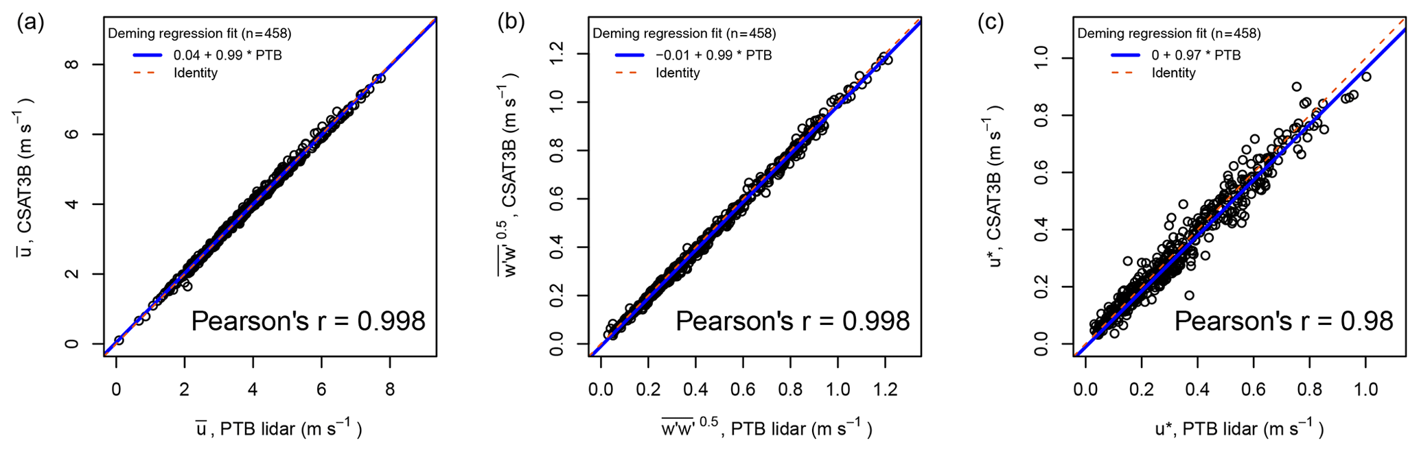
Figure 5Comparison for mean wind velocity (a), standard deviation of the vertical velocity component (b), and friction velocity (c), including the regression equation and correlation coefficient. The solid blue line indicates the Deming regression and the dashed red line indicates identity.
3.2 Spectral and co-spectral analysis
In the following section, we investigate the ensemble turbulence spectra of the three wind components, with a special focus on the ratios between them in the inertial subrange. This may help to shed more light on the reasons for the very good agreement between the CSAT3B and the PTB lidar measurements of . As can be seen in Fig. 7, all three wind components measured by the PTB lidar are afflicted by some noise at very high frequencies. In addition, the w spectra show a dampening of the signal at high frequencies. The CSAT3B spectra follow the theoretical power law very well across the entire inertial subrange in all three wind components. There are no signs of noise, aliasing, or high-frequency dampening in the spectra (Fig. 7).
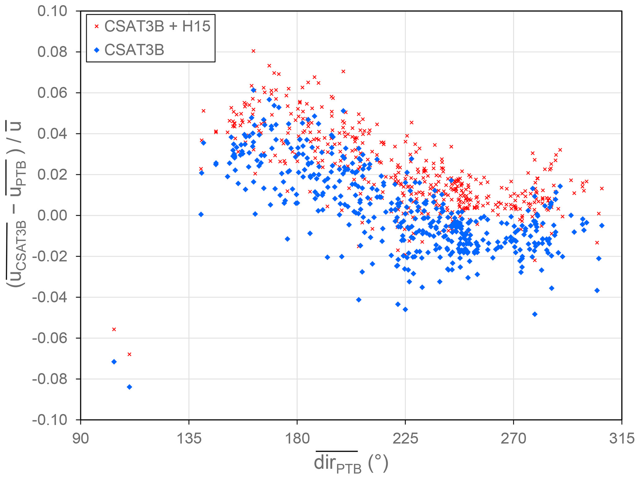
Figure 6Differences in wind velocity measurements between the two instruments , normalized by the mean wind velocity in versus the wind direction dir. The CSAT3 data are shown with and without the H15 correction.
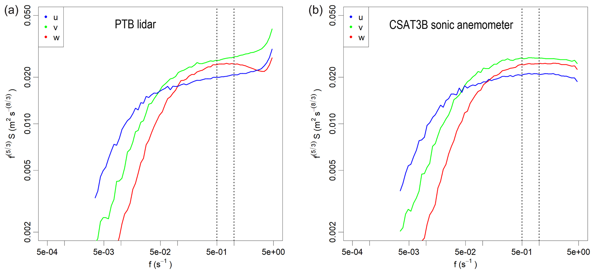
Figure 7Ensemble turbulence spectra of the three wind components u, v, and w, premultiplied by the frequency f(5∕3), so that the theoretical power law appears as a horizontal line. The spectra of the PTB lidar data are shown in (a) and the spectra of the CSAT3B data are shown in (b). The dashed vertical lines indicate the range between 0.5 and 1 s−1 in the inertial subrange for which the spectral ratios were calculated. Note that the deviations from the expected behaviour in the inertial subrange appear larger than at lower frequencies due to the pre-multiplication.
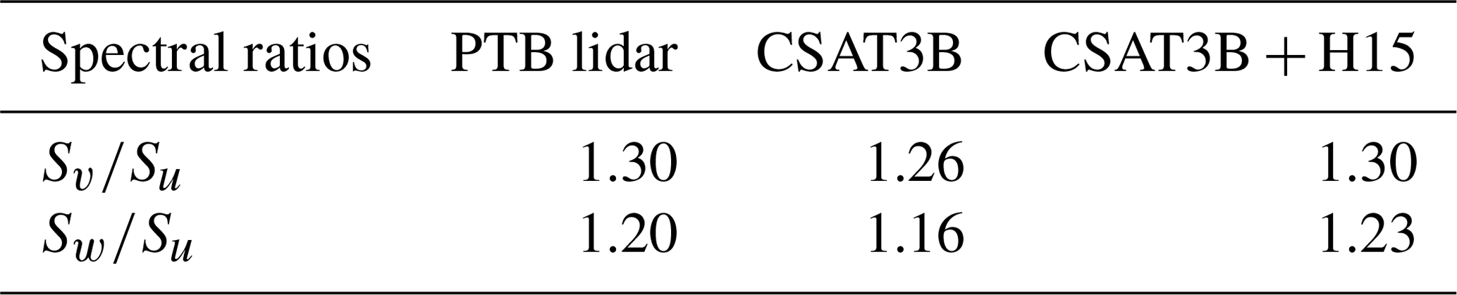
In addition to the power law, a spectral ratio of 4∕3 has been theoretically derived for Sv∕Su and Sw∕Su in the inertial subrange (Kaimal and Finnigan, 1994). We generally find smaller ratios for both instruments, while the ratios measured by the PTB lidar are generally larger than for the CSAT3B by a few percent (Table 2). We also find that the Sv∕Su ratios are generally larger than those for Sw∕Su. The lower Sw∕Su ratios have been interpreted as an indicator for probe-induced flow distortion (Peña et al., 2019), which is in line with our findings since the flow-distortion-free lidar measurements show larger values. However, even these flow-distortion-free data do not reach the theoretical value of 4∕3 for Sv∕Su and even less so for Sw∕Su. Hence, we suspect that this theoretical value was probably not fulfilled in reality for the ensemble spectrum, presumably because the turbulence was not quite isotropic under all atmospheric conditions during the measurement period, which can happen due to different reasons (Brugger et al., 2018; Stiperski and Calaf, 2018). In comparison with the uncorrected CSAT3 measurements of Peña et al. (2019), our CSAT3B data show slightly smaller Sv∕Su ratios of 1.26 versus 1.32 and 1.34, while the Sw∕Su ratios are slightly larger, being 1.16 versus 1.13 and 1.07 for their two data sets. It is interesting to note that after the application of the H15 correction, which is supposed to correct for flow distortion effects, the spectral ratio indeed agrees better with the theoretical value of 4∕3 and with the PTB lidar values than without the correction (Table 2).
Table 2Ratios between the spectral densities of the different wind components in the inertial subrange (at frequencies between 0.5 and 1 s−1) measured by the lidar and the sonic anemometer, with and without the H15 flow distortion correction. Note that both ratios Sv∕Su and Sw∕Su should theoretically be 4∕3 assuming isotropic turbulence (Kaimal and Finnigan, 1994).
As mentioned above, all the turbulence statistics of the PTB lidar are corrected for path-averaging effects according to Moore (1986) using a length of 0.05 m. Since the underlying analytical transfer function might not necessarily be correct for this instrument, we also determined the low-pass filtering transfer function empirically based on the ensemble spectrum of w. We found a cut-off frequency of 4 s−1, which results in an increase of by ca. 0.25 %, when applied as part of the Moore correction, compared to the value for the path averaging correction for 0.05 m measurement length. This small uncertainty adds confidence to the suitability of the PTB lidar for serving as absolute reference for in this comparison. Significant blue or white noise in Sw measured by the PTB lidar was not detected, either. In addition, we also calculated the turbulent statistics of the PTB lidar and the CSAT3B without any low-pass filtering correction whatsoever, and the results for show some small differences in comparison to the Moore-corrected data (Table 1), e.g. the bias is slightly smaller by 0.001 m s−1, while the RMSE is slightly larger by 0.003 m s−1. This shows that the effect of the low-pass correction is generally small because of the relatively large measurement height of 30 m.
Obviously, the results of this intercomparison partially contradict the findings of H15, Frank et al. (2016), and Huq et al. (2017), who advocate the need of a flow distortion correction on on the order of several percent. However, these previous field intercomparisons only compared different sonic anemometers with each other, partially with different sensor geometries, but none of them can be considered flow distortion free to the same extent as the bistatic Doppler lidar. It remains unclear why the numerical simulations of Huq et al. (2017) detect an underestimation of by 3 %–7 % for the CSAT3, when we see deviations of approximately 1 % in this field experiment. Perhaps the numerical simulations were not turbulent enough and thus the wake effects are stronger than under fully developed turbulent conditions in the field. Generally, wake effects depend on the Reynolds number and the wake extent is reduced suddenly at the transition from laminar to turbulent flow (e.g. Williamson, 1996). This is also the reason why it is problematic to transfer quasi-laminar wind tunnel calibrations to real-world turbulence (Högström and Smedman, 2004). Therefore, we believe that this explains the differences between our field study and previous wind-tunnel-based and numerical experiments (Grare et al., 2016; Huq et al., 2017), and we expect that the field experiment has more validity in principle, since sonic anemometers are normally used in the field.
Nevertheless, our results show that an azimuth-dependent flow distortion correction is indeed needed for obtaining more accurate measurements of the mean wind velocity of the CSAT3B (Sect. 3.1, Fig. 6). Further field comparisons with the PTB lidar or more realistic LES studies would be needed to this end. Moreover, it is generally preferable to minimize flow distortion errors to begin with through clever design of the instrument, e.g. by increasing the ratio between path length and transducer diameter, than relying on the transferability of wind-tunnel-based correction models to real-world conditions.
We found that the H15 flow distortion correction improves the u∗ comparison with the PTB lidar considerably, but why is only u∗ improved and not and ? An analysis of the Couw co-spectra shows that the CSAT3B deviates from the expected power law behaviour in the inertial subrange at frequencies (Fig. 8). It can also be seen that the H15 correction slightly increases the co-spectral energy across the entire range of frequencies. However, the too steep drop-off of the CSAT3B ensemble co-spectrum is not improved effectively. Hence, our analysis shows that the H15 correction results in improved the comparison of the u∗ values, but the ensemble co-spectrum shows that this improvement occurred for the wrong reasons. As a consequence, the observed behaviour of this correction for u∗ may potentially be site-specific and not universally transferable. Nevertheless, we would like to recall here that the underestimation of u∗ measured by the CSAT3B is only by a few percent, so that the accuracy of these uncorrected measurements is still sufficient for many applications.
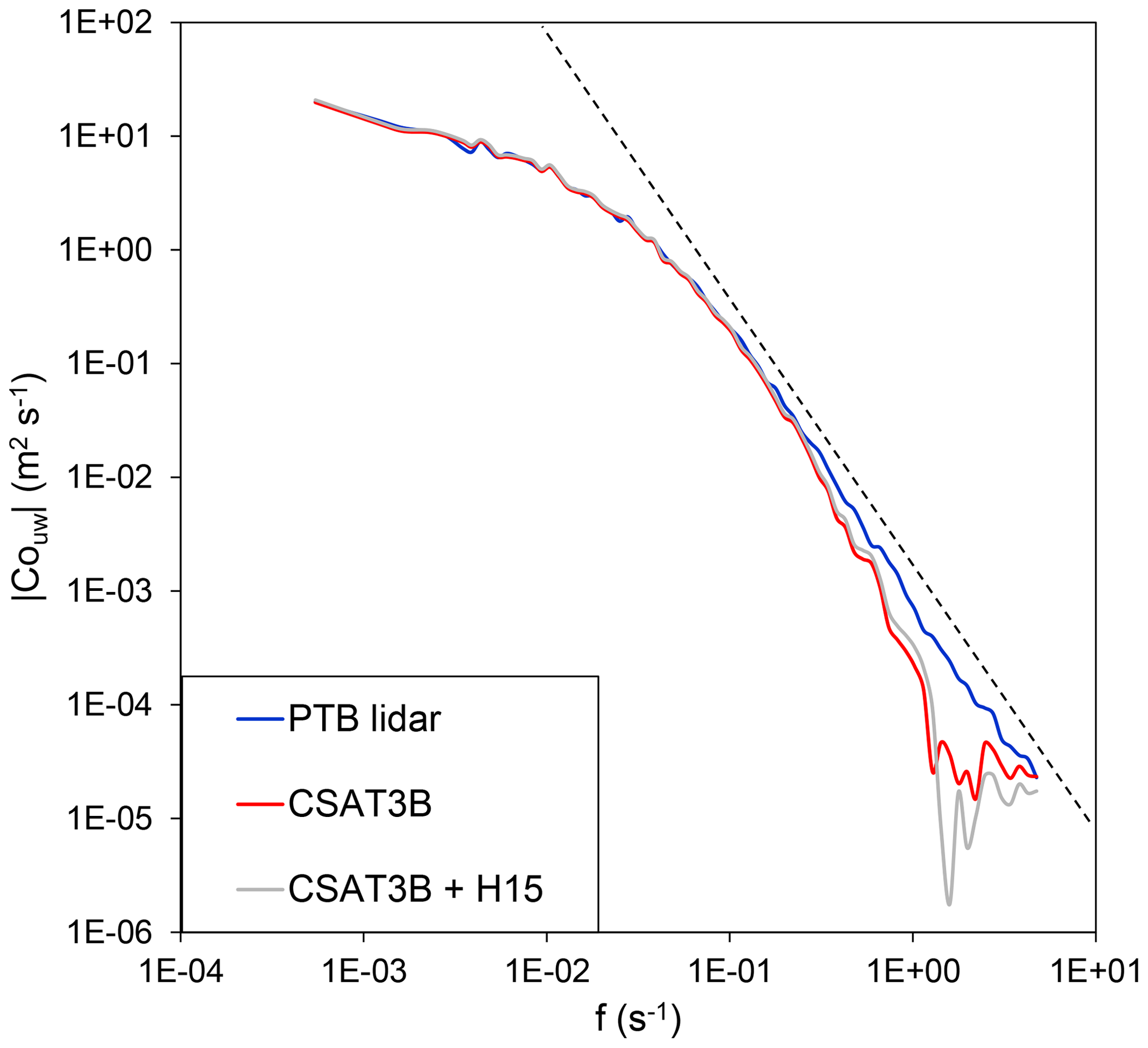
Figure 8Ensemble co-spectra between u and w (absolute value) based on turbulence measurements from the PTB lidar and the CSAT3B sonic anemometer. The dashed line indicates the theoretical power law in the inertial subrange.
We presented the results of a field intercomparison experiment, comparing the measurements of turbulence statistics in the atmospheric surface layer of a CSAT3B sonic anemometer and a novel bistatic Doppler lidar, which has been recently developed by PTB. Spectral analysis of the high-frequency data shows that the PTB lidar has some minor noise at high frequencies in all three wind components. In addition, w is slightly dampened at high frequencies, probably due to path length averaging, which can be corrected by a low-pass filtering correction normally applied for sonic anemometers (Moore, 1986). Nevertheless, this newly developed instrument is well suited for serving as independent reference in measuring turbulent statistics in the atmospheric surface layer due to its traceability to laser Doppler anemometer measurements in a wind tunnel and its completely unobstructed measurement volume.
Our comparison shows a very good agreement between both instruments for the measurement of and . Nevertheless, our results for spectral ratios between w and u confirm that the CSAT3B is somewhat affected by flow distortion in the measurement of . Moreover, u∗ from the CSAT3B is about 3 % too low compared to the PTB lidar, which is explained by the too steep drop-off of the Couw co-spectrum. We also evaluated whether the overall accuracy of the CSAT3B measurements can be improved by the H15 flow distortion correction, and our results indicate that this method increases the spectral energy across the entire range of frequencies equally and does not appropriately correct the CSAT3B data in the inertial subrange. It leads to an overestimation of , and it does not correct for the wind-direction-dependent error of . Based on these results, we conclude that the probe-induced flow distortion issue of sonic anemometers warrants further investigation in the future to effectively correct general measurements of scalar fluxes.
Since any systematic effects in the measurement of usually directly translate into errors in eddy-covariance flux measurements, the findings of this study are also relevant with respect to the energy balance closure problem (Stoy et al., 2013) and the accuracy of any trace gas flux measurement (Foken et al., 2011; Wilson et al., 2002). In this context, we can state that the very good agreement in the measurements of both instruments indicates that a probe-induced flow distortion error of the CSAT3B sonic anemometer contributes only very little to the observed systematic underestimation of scalar fluxes using the eddy-covariance method.
In summary, the agreement of all variables tested in this comparison experiment is at least as good as or better than that between two adjacent sonic anemometers (Mauder and Zeeman, 2018). This indicates that both instruments are very precise devices for measuring turbulence statistics, particularly for vertical scalar fluxes. Considering the findings of the intercomparison experiment of Mauder and Zeeman (2018), we conclude that the other sonic anemometers tested in that study are also suitable for general flux measurements within the range of comparability and bias described in that study. However, our spectral analysis shows that the bistatic Doppler lidar developed by PTB is slightly more accurate, particularly for measurements of friction velocity and the momentum flux.
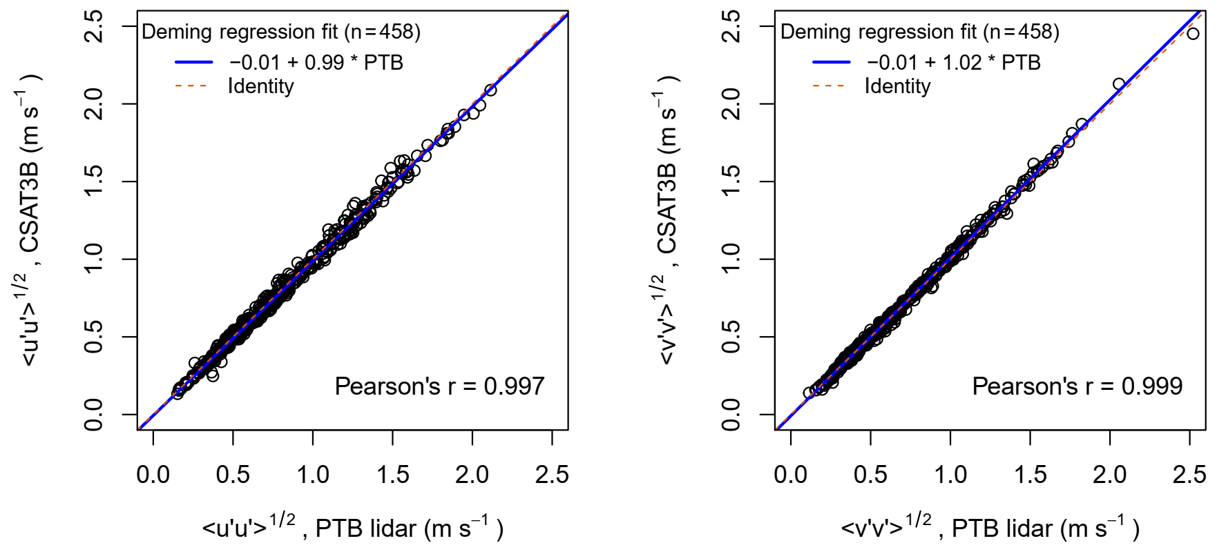
Figure A1Comparison for the standard deviation of the u velocity component (a) and the standard deviation of the v velocity component (b), including the regression equation and correlation coefficient. The solid blue line indicates the Deming regression and the dashed red line indicates identity. For , the bias is −0.008 m s−1 and RMSE is 0.028 m s−1, and for , the bias is 0.003 m s−1 and RMSE is 0.018 m s−1.
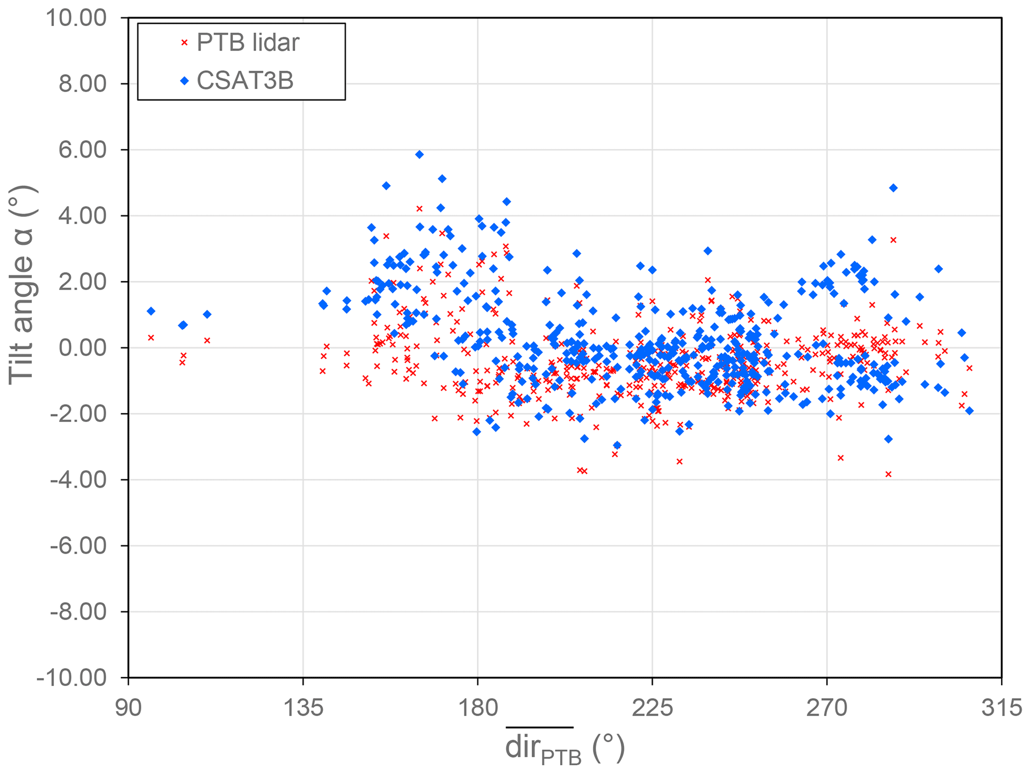
Figure A2Tilt angles α of the double rotation method on the y axis, forcing , as a function of the mean wind direction.
For completeness, we show the comparison for the standard deviations of u and v between the CSAT3B and the PTB lidar measurements in Fig. A1. The overall agreement is very good.
Tilt angles of the double rotation method as a function of wind direction can provide an indication about the potential misalignment of the instruments, which has been corrected for by this coordinate rotation as part of the post-processing. As expected, tilt angles of the PTB lidar are generally smaller than those of the CSAT3B (Fig. A2).
Sonic anemometer and Doppler lidar data are available upon request to Matthias Mauder (matthias.mauder@kit.edu).
MM and IV operated the sonic anemometer, and ME, CG, SO, and PW operated the Doppler lidar and pre-processed its 10 Hz raw data. MM calculated turbulence statistics, including the relevant corrections based on the raw sonic anemometer and Doppler lidar data, and calculated the statistical metrics for the intercomparison. LW and MM conducted the (co-spectral) analysis. MM wrote Sects. 1, 2.4, 2.5, 3, and 4; IB wrote Sect. 2.1.1; ME wrote Sect. 2.1.2; IV wrote Sect. 2.2; JT wrote Sect. 2.3; and LW wrote Sect. 2.6. All coauthors provided comments and suggestions on a previous version of this paper.
The authors declare that they have no conflict of interest.
We acknowledge Mathias Herbst of the DWD Zentrum für Agrarmeteorologische Forschung in Braunschweig for providing logistical support during the measurement campaign, and we thank the Thünen-Institut in Braunschweig for providing the field site for this experiment. The equipment for study has been financially supported in part by the Helmholtz initiative “Modular Observations Solutions for Earth Systems (MOSES)”. We thank Jamie Smidt (KIT) for checking the English grammar and spelling.
The article processing charges for this open-access publication were covered by a Research Centre of the Helmholtz Association.
This paper was edited by Szymon Malinowski and reviewed by John Frank and one anonymous referee.
Aubinet, M., Grelle, A., Ibrom, A., Rannik, Ü., Moncrieff, J., Foken, T., Kowalski, A. S., Martin, P. H., Berbigier, P., Bernhofer, Ch., Clement, R., Elbers, J., Granier, A., Grünwald, T., Morgenstern, K., Pilegaard, K., Rebmann, C., Snijders, W., Valentini, R., and Vesala, T.: Estimates of the annual net carbon and water exchange of forest: the EUROFLUX methodology, Adv. Ecol. Res., 30, 113–117, https://doi.org/10.1016/S0065-2504(08)60018-5, 2000.
Aubinet, M., Vesala, T., and Papale, D. (eds.): Eddy Covariance – A Practical Guide to Measurement and Data Analysis, Springer, Dordrecht, 2012.
Bingöl, F., Mann, J., and Foussekis, D.: Conically scanning lidar error in complex terrain, Meteorol. Z., 18, 189–195, https://doi.org/10.1127/0941-2948/2009/0368, 2009.
Bradley, S.: Wind speed errors for LIDARs and SODARs in complex terrain, IOP Conf. Ser. Earth Environ. Sci., 1, 012061, https://doi.org/10.1088/1755-1307/1/1/012061, 2008.
Brugger, P., Träumner, K., and Jung, C.: Evaluation of a procedure to correct spatial averaging in turbulence statistics from a doppler lidar by comparing time series with an ultrasonic anemometer, J. Atmos. Ocean. Technol., 33, 2135–2144, https://doi.org/10.1175/JTECH-D-15-0136.1, 2016.
Brugger, P., Katul, G. G., De Roo, F., Kröniger, K., Rotenberg, E., Rohatyn, S., and Mauder, M.: Scalewise invariant analysis of the anisotropic Reynolds stress tensor for atmospheric surface layer and canopy sublayer turbulent flows, Phys. Rev. Fluids, 3, 054608, https://doi.org/10.1103/PhysRevFluids.3.054608, 2018.
Drain, L. E.: The Laser Doppler Technique, John Wiley and Sons Ltd., Chichester, UK, 1980.
Eder, F., De Roo, F., Rotenberg, E., Yakir, D., Schmid, H. P., and Mauder, M.: Secondary circulations at a solitary forest surrounded by semi-arid shrubland and its impact on eddy-covariance measurements, Agr. Forest Meteorol., 211–212, 115–127, https://doi.org/10.1016/j.agrformet.2015.06.001, 2015.
Elzhov, T. V., Mullen, K. M., Spiess, A.-N., and Bolker, B.: minpack.lm: R Interface to the Levenberg-Marquardt Nonlinear Least-Squares Algorithm Found in MINPACK, Plus Support for Bounds, [online] Available from: https://cran.r-project.org/package=minpack.lm, 2016.
Foken, T. and Oncley, S. P.: Workshop on instrumental and methodical problems of land surface flux measurements, B. Am. Meteorol. Soc., 76, 1191–1193, 1995.
Foken, T., Aubinet, M., Finnigan, J. J., Leclerc, M. Y., Mauder, M., and Paw U, K. T.: Results of a panel discussion about the energy balance closure correction for trace gases, B. Am. Meteorol. Soc., 92, ES13–ES18, https://doi.org/10.1175/2011BAMS3130.1, 2011.
Frank, J. M., Massman, W. J., and Ewers, B. E.: Underestimates of sensible heat flux due to vertical velocity measurement errors in non-orthogonal sonic anemometers, Agr. Forest Meteorol., 171–172, 72–81, https://doi.org/10.1016/j.agrformet.2012.11.005, 2013.
Frank, J. M., Massman, W. J., Swiatek, E., Zimmerman, H. A., and Ewers, B. E.: All sonic anemometers need to correct for transducer and structural shadowing in their velocity measurements, J. Atmos. Ocean. Technol., 33, 149–167, https://doi.org/10.1175/JTECH-D-15-0171.1, 2016.
Fratini, G. and Mauder, M.: Towards a consistent eddy-covariance processing: an intercomparison of EddyPro and TK3, Atmos. Meas. Tech., 7, 2273–2281, https://doi.org/10.5194/amt-7-2273-2014, 2014.
Fratini, G., Ibrom, A., Arriga, N., Burba, G., and Papale, D.: Relative humidity effects on water vapour fluxes measured with closed-path eddy-covariance systems with short sampling lines, Agr. Forest Meteorol., 165, 53–63, https://doi.org/10.1016/j.agrformet.2012.05.018, 2012.
Gottschall, J., Courtney, M. S., Wagner, R., Jørgensen, H. E., and Antoniou, I.: Lidar profilers in the context of wind energy – a verification procedure for traceable measurements, Wind Energy, 15, 147–159, https://doi.org/10.1002/we.518, 2012.
Grare, L., Lenain, L., and Melville, W. K.: The Influence of Wind Direction on Campbell Scientific CSAT3 and Gill R3-50 Sonic Anemometer Measurements, J. Atmos. Ocean. Technol., 33, 2477–2497, https://doi.org/10.1175/JTECH-D-16-0055.1, 2016.
Harris, M., Constant, G., and Ward, C.: Continuous-wave bistatic laser Doppler wind sensor, Appl. Opt., 40, 1501–1506, https://doi.org/10.1364/AO.40.001501, 2001.
Högström, U. and Smedman, A. S.: Accuracy of sonic anemometers: Laminar wind-tunnel calibrations compared to atmospheric in situ calibrations against a reference instrument, Bound.-Lay. Meteorol., 111, 33–54, https://doi.org/10.1023/B:BOUN.0000011000.05248.47, 2004.
Højstrup, J.: A simple model for the adjustment of velocity spectra in unstable conditions downstream of an abrupt change in roughness and heat flux, Bound.-Lay. Meteorol., 21, 341–356, https://doi.org/10.1007/BF00119278, 1981.
Horst, T. W., Semmer, S. R., and Maclean, G.: Correction of a Non-orthogonal, Three-Component Sonic Anemometer for Flow Distortion by Transducer Shadowing, Bound.-Lay. Meteorol., 155, 371–395, https://doi.org/10.1007/s10546-015-0010-3, 2015.
Horst, T. W., Vogt, R., and Oncley, S. P.: Measurements of Flow Distortion within the IRGASON Integrated Sonic Anemometer and CO2/H2O Gas Analyzer, Bound.-Lay. Meteorol., https://doi.org/10.1007/s10546-015-0123-8, 2016.
Huq, S., De Roo, F., Foken, T., and Mauder, M.: Evaluation of Probe-Induced Flow Distortion of Campbell CSAT3 Sonic Anemometers by Numerical Simulation, Bound.-Lay. Meteorol., 165, https://doi.org/10.1007/s10546-017-0264-z, 2017.
Ibrom, A., Dellwik, E., Flyvbjerg, H., Jensen, N. O., and Pilegaard, K.: Strong low-pass filtering effects on water vapour flux measurements with closed-path eddy correlation systems, Agr. Forest Meteorol., 147, 140–156, 2007.
Kaimal, J.: Sonic Anemometer Measurement of Atmospheric Turbulence, in: Proceedings of the Dynamic Flow Conference 1978 on Dynamic Measurements in Unsteady Flows, edited by Hanson, B. W., Springer Netherlands, Dordrecht, pp. 551–565, 1979.
Kaimal, J. C. C. and Finnigan, J. J.: Atmospheric Boundary Layer Flows: Their Structure and Measurement, Oxford University Press, New York, 1994.
Kolmogorov, A. N.: The local structure of turbulence in incompressible viscous fluid for very large Reynolds numbers, C. R. Acad. Sci. URSS, 30, 301–305, 1941.
Loescher, H. W., Ocheltree, T., Tanner, B., Swiatek, E., Dano, B., Wong, J., Zimmerman, G., Campbell, J., Stock, C., Jacobsen, L., Shiga, Y., Kollas, J., Liburdy, J., and Law, B. E.: Comparison of temperature and wind statistics in contrasting environments among different sonic anemometer-thermometers, Agr. Forest Meteorol., 133, 119–139, https://doi.org/10.1016/j.agrformet.2005.08.009, 2005.
Manuilova, E., Schuetzenmeister, A., and Model, F.: mcr: Method Comparison Regression. [online] Available from: https://cran.r-project.org/package=mcr, 2014.
Mauder, M. and Foken, T.: Eddy-Covariance Software TK3, available at: http://dx.doi.org/10.5281/zenodo.20349, 2015.
Mauder, M. and Zeeman, M. J.: Field intercomparison of prevailing sonic anemometers, Atmos. Meas. Tech., 11, 249–263, https://doi.org/10.5194/amt-11-249-2018, 2018.
Mauder, M., Oncley, S. P., Vogt, R., Weidinger, T., Ribeiro, L., Bernhofer, C., Foken, T., Kohsiek, W., De Bruin, H. A. R., and Liu, H.: The energy balance experiment EBEX-2000. Part II: Intercomparison of eddy-covariance sensors and post-field data processing methods, Bound.-Lay. Meteorol., 123, 29–54, https://doi.org/10.1007/s10546-006-9139-4, 2007.
Mauder, M., Cuntz, M., Drüe, C., Graf, A., Rebmann, C., Schmid, H. P., Schmidt, M., and Steinbrecher, R.: A strategy for quality and uncertainty assessment of long-term eddy-covariance measurements, Agr. Forest Meteorol., 169, 122–135, https://doi.org/10.1016/j.agrformet.2012.09.006, 2013.
Moore, C. J.: Frequency response corrections for eddy correlation systems, Bound.-Lay. Meteorol., 37, 17–35, https://doi.org/10.1007/BF00122754, 1986.
Newman, J. F., Klein, P. M., Wharton, S., Sathe, A., Bonin, T. A., Chilson, P. B., and Muschinski, A.: Evaluation of three lidar scanning strategies for turbulence measurements, Atmos. Meas. Tech., 9, 1993–2013, https://doi.org/10.5194/amt-9-1993-2016, 2016.
Oertel, S., Eggert, M., Gutsmuths, C., Wilhelm, P., Müller, H., and Többen, H.: Validation of three-component wind lidar sensor for traceable highly resolved wind vector measurements, J. Sensors Sens. Syst., 8, 9–17, https://doi.org/10.5194/jsss-8-9-2019, 2019.
Pearson, G., Davis, F., Collier, C., Davies, F., Collier, C., Davis, F., and Collier, C.: An analysis of the performance of the UFAM pulsed Doppler Lidar for observing the Boundary Layer, J. Atmos. Ocean. Technol., 26, 240–249, https://doi.org/10.1175/2008JTECHA1128.1, 2009.
Peña, A., Hasager, C. B., Gryning, S.-E., Courtney, M., Antoniou, I., and Mikkelsen, T.: Offshore wind profiling using light detection and ranging measurements, Wind Energy, 12, 105–124, 2009.
Peña, A., Dellwik, E., and Mann, J.: A method to assess the accuracy of sonic anemometer measurements, Atmos. Meas. Tech., 12, 237–252, https://doi.org/10.5194/amt-12-237-2019, 2019.
Stiperski, I. and Calaf, M.: Dependence of near-surface similarity scaling on the anisotropy of atmospheric turbulence, Q. J. R. Meteorol. Soc., 144, 641–657, https://doi.org/10.1002/qj.3224, 2018.
Stoy, P. C., Mauder, M., Foken, T., Marcolla, B., Boegh, E., Ibrom, A., Arain, M. A. A., Arneth, A., Aurela, M., Bernhofer, C., Cescatti, A., Dellwik, E., Duce, P., Gianelle, D., van Gorsel, E., Kiely, G., Knohl, A., Margolis, H., Mccaughey, H., Merbold, L., Montagnani, L., Papale, D., Reichstein, M., Saunders, M., Serrano-Ortiz, P., Sottocornola, M., Spano, D., Vaccari, F., and Varlagin, A.: A data-driven analysis of energy balance closure across FLUXNET research sites: The role of landscape-scale heterogeneity, Agr. Forest Meteorol., 171, 137–152, https://doi.org/10.1016/j.agrformet.2012.11.004, 2013.
Stull, R. B.: An Introduction to Boundary Layer Meteorology, Kluwer Academic Publishers, Dordrecht, 666 pp., 1988.
Tambke, J., Focken, U., Lange, M., Wolff, J.-O., and Bye, J. A. T.: Forecasting offshore wind speeds above the North Sea, Wind Energy, 8, 3–16, 2005.
Williamson, C. H. K.: Vortex Dynamics in the Cylinder Wake, Annu. Rev. Fluid Mech., 28, 477–539, https://doi.org/10.1146/annurev.fl.28.010196.002401, 1996.
Wilson, K., Goldstein, A., Falge, E., Aubinet, M., Baldocchi, D., Berbigier, P., Bernhofer, C., Ceulemans, R., Dolman, H., and Field, C.: Energy balance closure at FLUXNET sites, Agr. Forest Meteorol., 113, 223–243, https://doi.org/10.1016/S0168-1923(02)00109-0, 2002.
Wyngaard, J. C.: Flow-distortion effects on scalar flux measurements in the surface layer: Implications for sensor design, Bound.-Lay. Meteorol., 42, 19–26, https://doi.org/10.1007/BF00119872, 1988.
Wyngaard, J. C. and Zhang, S.-F. F.: Transducer-Shadow Effects on Turbulence Spectra Measured by Sonic Anemometers, J. Atmos. Ocean. Technol., 2, 548–558, 1985.
Zhang, S. F., Wyngaard, J. C., Businger, J. A., and Oncley, S. P.: Response characteristics of the U.W. sonic anemometer, J. Atmos. Ocean. Technol., 3, 315–323, 1986.