the Creative Commons Attribution 4.0 License.
the Creative Commons Attribution 4.0 License.
 | 24 Feb 2021
Model estimations of geophysical variability between satellite measurements of ozone profiles
Patrick E. Sheese
Chris D. Boone
Doug A. Degenstein
Felicia Kolonjari
David Plummer
Douglas E. Kinnison
Patrick Jöckel
Thomas von Clarmann
In order to validate satellite measurements of atmospheric composition, it is necessary to understand the range of random and systematic uncertainties inherent in the measurements. On occasions where measurements from two different satellite instruments do not agree within those estimated uncertainties, a common explanation is that the difference can be assigned to geophysical variability, i.e., differences due to sampling the atmosphere at different times and locations. However, the expected geophysical variability is often left ambiguous and rarely quantified. This paper describes a case study where the geophysical variability of O3 between two satellite instruments – ACE-FTS (Atmospheric Chemistry Experiment – Fourier Transform Spectrometer) and OSIRIS (Optical Spectrograph and InfraRed Imaging System) – is estimated using simulations from climate models. This is done by sampling the models CMAM (Canadian Middle Atmosphere Model), EMAC (ECHAM/MESSy Atmospheric Chemistry), and WACCM (Whole Atmosphere Community Climate Model) throughout the upper troposphere and stratosphere at times and geolocations of coincident ACE-FTS and OSIRIS measurements. Ensemble mean values show that in the lower stratosphere, O3 geophysical variability tends to be independent of the chosen time coincidence criterion, up to within 12 h; and conversely, in the upper stratosphere geophysical variation tends to be independent of the chosen distance criterion, up to within 2000 km. It was also found that in the lower stratosphere, at altitudes where there is the greatest difference between air composition inside and outside the polar vortex, the geophysical variability in the southern polar region can be double of that in the northern polar region. This study shows that the ensemble mean estimates of geophysical variation can be used when comparing data from two satellite instruments to optimize the coincidence criteria, allowing for the use of more coincident profiles while providing an estimate of the geophysical variation within the comparison results.
- Article
(3912 KB) - Full-text XML
- BibTeX
- EndNote


A significant uncertainty when comparing concentrations of trace species measured from different satellite instruments is the difference due to the satellites sampling the atmosphere at different times and locations (“coincident” measurements are never truly coincident). This uncertainty can be called “geophysical variability”, “natural variability”, or “coincident location uncertainty” – this study uses the term geophysical variability. Loew et al. (2017), when reviewing the methods and techniques used in Earth observation data validation, wrote “Collocated measurements should be close to each other relative to the spatiotemporal scale on which the variability of the geophysical field becomes comparable to the measurement uncertainties”, and it is assumed that the “spatiotemporal scale” (coincidence criteria) that will result in geophysical variability on the order of the measurement uncertainties is known. However, it is often the case that validation studies involving satellite-based atmospheric measurements will choose coincidence criteria without discussing the geophysical justification of the criteria.
There are many validation studies that try to either estimate or limit geophysical variability using various techniques. One common method for reducing temporal variability is to make use of chemical models in order to diurnally scale the measurements to a common local time (e.g., Sheese et al., 2016, and references therein). Two methods that are similar to each other are the trajectory mapping (Morris et al., 1995) and the target hunting techniques (Danilin et al., 2000), which involve tracking air parcels using forward and/or back trajectories when comparing two different data sets. These have been shown to be reliable tools for validation (e.g., Bacmeister et al., 1999; Morris et al., 2000; Danilin et al., 2002a, b; Liu et al., 2013) without introducing large sources of uncertainty; however it can be computationally expensive to create trajectories for multiple instrument data sets. Verhoelst et al. (2015) coupled a numerical weather forecast model with an ozone tracer model to create a high spatial-resolution observing system simulation experiment (OSSE) in order to model coincident mismatch uncertainty (as well as vertical smoothing uncertainty) between satellite- and ground-based measurements. Although it was shown that the OSSE could successfully represent the geophysical variability, as discussed by Loew et al. (2017), this method would likely not be suitable for atmospheric targets that exhibit greater geophysical variability than O3. Simple statistical or chemistry models have also been used in studies to assess geophysical variability between atmospheric measurements (e.g., Aghedo et al., 2011; Guan et al., 2013; Toohey et al., 2013; Fassò et al., 2014; Sofieva et al., 2014; Millán et al., 2016).
In a similar, yet simplified, approach to Verhoelst et al. (2015), this study makes use of readily available output from three climate models that relaxed various meteorological fields using specified dynamics: the Canadian Middle Atmosphere Model (CMAM), the ECHAM/MESSy (European Centre Hamburg general circulation model, Modular Earth Sub-model System) Atmospheric Chemistry (EMAC) model, and the Whole Atmosphere Community Chemistry Model (WACCM). It is important to note that this study is not intended to validate either the ACE-FTS (Atmospheric Chemistry Experiment – Fourier Transform Spectrometer) or OSIRIS (Optical Spectrograph and InfraRed Imaging System) O3 data products. This is a case study that makes use of ACE-FTS and OSIRIS geolocation data and O3 products to demonstrate how readily available data from nudged climate models can be used to estimate large-scale geophysical variability between satellite measurements of atmospheric trace species and how they can be used to make informed decisions when choosing coincidence criteria in a validation study. In this study, given the horizontal resolution of the three climate models that were used, large-scale variability is on the order of 200–300 km, which is on the order of the atmospheric path length of a limb-viewing instrument at the tangent height.
The following section describes the satellite and model data sets used in this study, and Sect. 3 describes the methodology for sampling the model data and how the data sets are compared to one another. Section 4 discusses the resulting simulated geophysical variability and how those results can potentially be used to help improve validation studies. A summary is then given in Sect. 5.
2.1 ACE-FTS on SCISAT
The ACE-FTS instrument (Bernath et al., 2005) is a solar occultation instrument on board the Canadian satellite SCISAT, which was launched into a highly inclined, non-sun-synchronous orbit in 2003. Since February 2004, ACE-FTS has been making observations of Earth's limb, providing profiles of atmospheric temperature and concentrations of over 30 trace species between altitudes of ∼ 5 and 150 km. The instrument is a high spectral-resolution (0.02 cm−1) infrared spectrometer detecting solar radiation between 750 and 4400 cm−1.
The O3 retrieval algorithm, described by Boone et al. (2005, 2013), is a global least-squares fitting technique that uses Levenberg–Marquardt iteration to converge on a solution without the need of a priori information. Version 3.5/3.6 data are used in this study, where the forward modelled spectra in 40 different microwindows between 829 and 2673 cm−1 are calculated using spectral parameters from the HITRAN 2004 (Rothman et al., 2005) database with some updates, as described by Boone et al. (2013). Ozone is retrieved between 5 and 95 km assuming horizontal homogeneity, and CFC-12, HCFC-22, CFC-11, N2O, CH4, HCOOH, and H2O, along with various isotopologues, are simultaneously retrieved as interfering species. The reported statistical fitting error, described by Boone et al. (2005; 2013), is typically on the order of 2 %–3 % in the 10–15 km range and ∼ 1.5 %–2 % in the 15–55 km range. Dupuy et al. (2009) validated the ACE-FTS v2.2 ozone data set using correlative data from multiple satellite, ground-based, and balloon-based instruments, and Sheese et al. (2017) compared v3.5 O3 data to correlative satellite data. In the upper troposphere to middle stratosphere, ACE-FTS v3.5 O3 tends to exhibit a slight positive bias on the order of a few percent and, near 45–60 km, a positive bias on the order of 10 %–20 %.
2.2 OSIRIS on Odin
The OSIRIS instrument (Llewellyn et al., 2004) is a limb scatter detector on board the Odin satellite, which was launched into a sun-synchronous orbit in 2001 with a nominal ascending node of approximately 06:00 local time. Since November 2001, OSIRIS has been observing Earth's limb, producing standard data products of O3 and NO2 profiles between altitudes of ∼ 7 and 60 km, as well as various other atmospheric research products. The optical spectrograph is a grating spectrometer measuring between 275 and 810 nm with a spectral resolution of ∼ 2 nm and a vertical field of view of ∼ 1 km at the tangent point.
The O3 retrieval algorithm is described by Bourassa et al. (2012) and uses a multiplicative algebraic reconstruction technique (Roth et al., 2007; Degenstein et al., 2009). Version 5.07 O3 data are used in this study, where pressure and temperature profiles are obtained from the European Centre for Medium-Range Weather Forecasts (ECMWF), and ozone is retrieved in number density, taking into account UV and visible absorption, and NO2 and aerosols are simultaneously retrieved as interfering species. The ECMWF pressure and temperature profiles are then used to convert the retrieved O3 densities to volume mixing ratios. The reported OSIRIS O3 uncertainties are typically on the order of 3 %–9 % in the 10–55 km range.
Adams et al. (2013) found that the v5.07 OSIRIS data were in excellent agreement with coincident Stratospheric Aerosol and Gas Experiment II (SAGE II) profiles throughout the stratosphere, typically within 5 %. Hubert et al. (2016) found there to be a statistically significant positive drift in the OSIRIS O3 data above 20 km with respect to ozonesonde and lidar data. The OSIRIS drift is on the order of 1 %–3 % per decade between ∼ 25 and 35 km and increases to 8 % per decade near 42 km; however, this drift has been corrected in the v5.10 release (Bourassa et al., 2018).
2.3 Model data
Three different models were used in this study: CMAM, EMAC, and WACCM, all of which used specified dynamics to relax, or “nudge”, different key atmospheric states (e.g., wind fields, temperature) to meteorological observations.
CMAM is a chemistry–climate model, described in detail by de Grandpré et al. (2000), Jonsson et al. (2004), and Scinocca et al. (2008). The CMAM30 simulation (McLandress et al., 2013), used in this study, is a 30-year run of the CMAM model with 6-hourly output from 1979 to 2010, on a 3.75∘ horizontal grid (linear T47 Gaussian grid). The model was run with 71 vertical levels up to 0.0007 hPa (∼ 95 km) with vertical resolution on the order of 1 km around the tropopause, increasing to ∼ 2.5 km in the mesosphere, and the data set used here is comprised of 6-hourly instantaneous model fields interpolated onto 63 constant pressure surfaces that span the full height range of the model. Below 1 hPa, temperatures and horizontal winds were nudged to 6-hourly values from ECMWF Interim Reanalysis (ERA-interim; Dee et al., 2011). CMAM simulations have been used in many studies to help understand the climatology and variations of stratospheric O3 and its effect on climate (e.g., Gillett et al., 2009; McLandress et al., 2011; Sakazaki et al., 2015; Froidevaux et al., 2019).
The global chemistry–climate model EMAC uses the general circulation model ECHAM version 5 as its base model in conjunction with MESSy version 2, which incorporates multiple sub-models, such as natural and anthropogenic emissions, land and ocean processes and interactions, and chemistry and transport (Jöckel et al., 2010, 2016). The simulations used in this study were on an approximate 2.8∘ horizontal grid (T42), with 90 vertical levels up to 0.01 hPa (∼ 80 km). Within the 30-year run (1980–2010), the calculated divergence, vorticity, temperature, and logarithm of surface pressure variables were nudged above the boundary layer up to 10 hPa (with transition layers) to ERA-interim data with nudging times between 6 and 48 h, depending on the variable. The data used in this study were from simulation RC1SD-base-10 (no nudging of global mean temperature), output every 5 h (Jöckel et al., 2016). Multiple studies focusing on O3 variations in the troposphere and stratosphere have used the EMAC model (e.g., Weber et al., 2011; Meul et al., 2014; Khosrawi et al., 2017).
WACCM is a climate chemistry model and is the atmospheric component of the National Center for Atmospheric Research's Community Earth System Model (Marsh et al., 2013). The simulations used in this study have horizontal resolutions of 1.9∘ latitude and 2.5∘ longitude and have 88 vertical levels up to 5.1 × 10⁻⁶ hPa (∼ 140 km). The model simulation spans 1979 to 2013, and below 50 km the temperature, pressure, zonal and meridional wind, and surface stress variables were nudged to NASA's Modern Era Retrospective-Analysis for Research and Applications (MERRA) reanalysis data (Rienecker et al., 2011) with a 50 h relaxation time constant. The WACCM model has been widely used to study O3 variability throughout the atmosphere (e.g., Merkel et al., 2011; Brakebusch et al., 2013; Chandran et al., 2014).
Another set of WACCM simulations was used in this study, with the same setup, the only difference being that the output model data were directly output at the ACE-FTS and OSIRIS observation times and geolocations (individual observation profiles were assumed to be at a single time, latitude, and longitude, taken as the 30 km tangent height values). The WACCM output at the instrument observed locations will from here onward be referred to as WACCMOL.
All three models used in this study are considered to be “state-of-the-art” stratosphere-resolving chemistry–climate models and regularly participate in multi-model intercomparisons, including the exhaustive model assessments performed for CCMVal-2 (SPARC CCMVal, 2010) and CCMI-1 (Morgenstern et al., 2017).
In this study, altitude-dependent values of latitude and longitude were used for the measured profiles; however time values were assumed to be constant throughout a profile, taken as the mid-point of the measurement time. ACE-FTS and OSIRIS profiles were considered to be coincident if they were measured within 12 h of each other and within 2000 km. In cases of multiple coincidences with a single profile, only the closest in latitude were chosen; hence each ACE-FTS profile has only one coincident OSIRIS profile and vice versa. Only data from 2004 to 2010 are used, as the latest start point out of all the data sets (model and instrument) was the ACE-FTS start of February 2004, and the CMAM and EMAC data sets both had the same earliest end point, December 2010.
In the following description the terms MOD and INST are used as general terms to indicate model and instrument values, respectively. The sampling of all three models (CMAM, EMAC, and WACCM) at satellite times and locations is done using the same methodology. First, for every instrument profile, the model O3 data closest in time to tINST on both sides are isolated and are spline-interpolated in log space from the native grid to a grid, where t is time, p is pressure, z is altitude, long is longitude, and lat is latitude. This is done using the retrieved ACE-FTS pressures, which are on a 1 km grid from 0.5 to 149.5 km. Since OSIRIS does not retrieve atmospheric pressure, the OSIRIS O3, time, latitude, and longitude profiles (in altitude) are spline-interpolated to the ACE-FTS grid and assumed to have the same pressure values as their coincident ACE-FTS profile. Due to using the ACE-FTS pressures, this study can be considered to be estimating the natural variability on common pressure levels, rather than on common altitude levels.
For each profile, the model data are then linearly interpolated from the grid to a grid at tINST. At each altitude, the (longMOD, latMOD) gridded data are then bilinearly interpolated to the longINST and latINST values at that altitude, using altitude-dependent geolocations (e.g., Kolonjari et al., 2018). This leads to model O3 data sampled at the instrument times and geolocations on a (zINST, tINST) grid. Outliers in the ACE-FTS data are filtered out using their quality flags, as per Sheese et al. (2015), and the corresponding data points are also removed from the corresponding OSIRIS and model data sets. The OSIRIS data were not filtered for outliers.
The estimated geophysical variability, as per the model data sets, was defined to be the 2σ standard deviation of the differences between simulated ACE-FTS values and simulated OSIRIS values (at each altitude):
In relative terms, the relative differences are calculated as the differences between ACE-FTS and OSIRIS divided by the overall mean of all ACE-FTS and OSIRIS values at that altitude:
where N is the number of coincident values at that altitude. The overall mean in the denominator was used in order to be consistent with Sheese et al. (2016, 2017), where it was used to minimize the effect of retrieved negative values. The relative geophysical variability was calculated as the 2σ standard deviation of the relative differences. The same equations were used for determining the relative differences and the 2σ variations between the actual ACE-FTS and OSIRIS measurements (replacing MOD in Eqs. 1 and 2 with INST).
4.1 Global comparisons
Coincidence criteria of within 6 h and 500 km were first chosen, yielding the profiles of mean O3 bias (ACE-FTS – OSIRIS) due to sampling and geophysical variability profiles (2σ variation) shown in Fig. 1. Also shown are the profiles of the actual measurement bias and 2σ variation of the differences at those criteria. All three models exhibit a small bias (within 0.02 ppmv, 0.5 %) between 12 and 29 km. Between 30 and 45 km, the model results indicate that ACE-FTS O3 values are expected to be systematically lower than OSIRIS. CMAM indicates a bias of up to ∼ 0.02 ppmv (0.5 %) in this region, EMAC indicates a bias of up to ∼ 0.06 ppmv (1.1 %), and WACCM indicates a bias of up to 0.13 ppmv (2.8 %). Above 48 km, all three models exhibit systematically larger concentrations of ACE-FTS O3 than OSIRIS O3. EMAC indicates a bias of up to ∼ 0.03 ppmv (2.1 %) in this region, CMAM indicates a bias of up to 0.05 ppmv (3.9 %), and WACCM indicates a bias of up to 0.10 ppmv (8.7 %). The more extreme values yielded by the WACCM simulations could in part be due to the finer horizontal resolution.
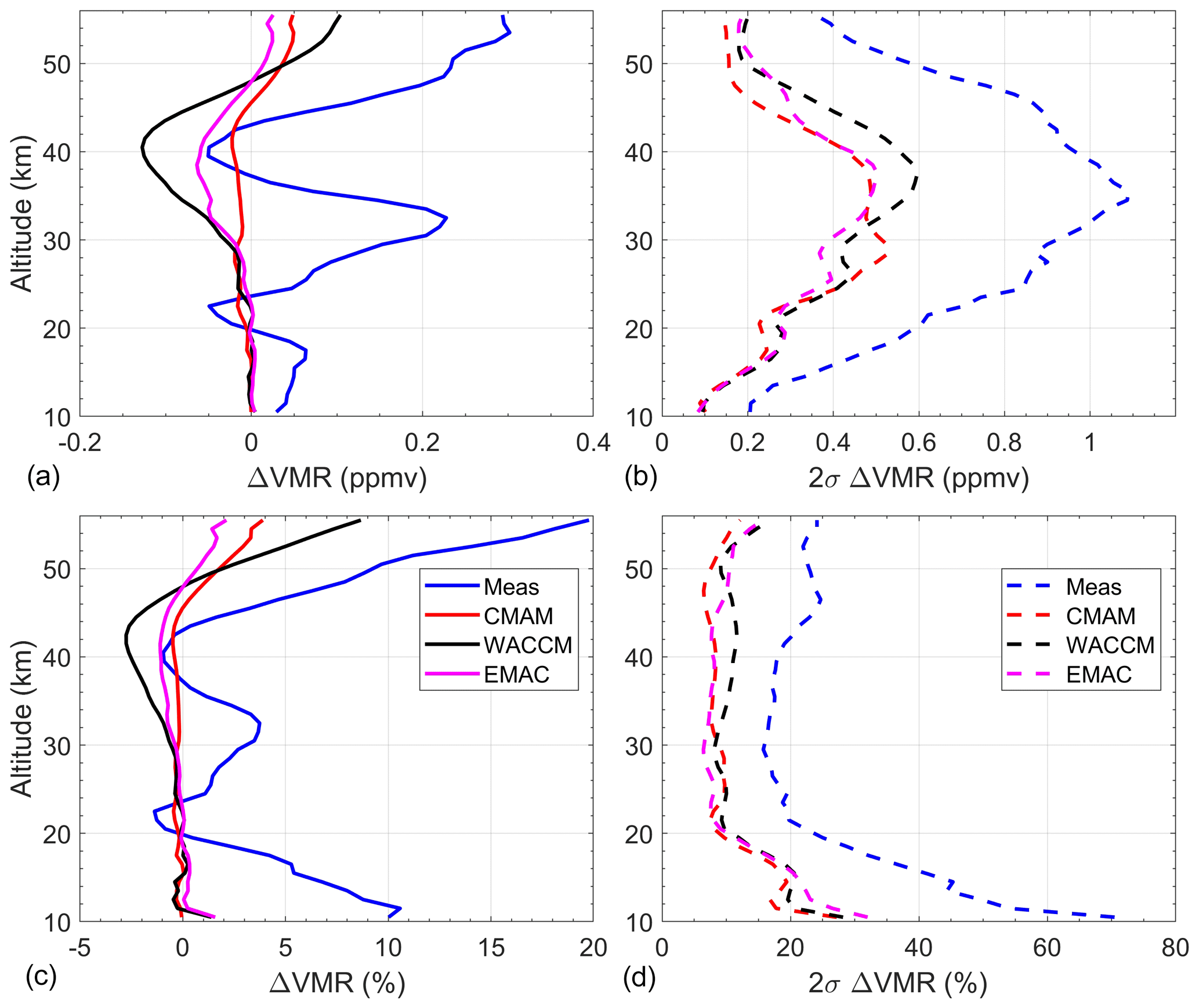
Figure 1Measured and simulated mean differences (a, c) between ACE-FTS and OSIRIS O3 and the corresponding 2σ variability (b, d). Profiles for all available times and latitudes with coincidence criteria of within 6 h and 500 km are used. Results shown for the differences (a, b) and relative differences (c, d).
All three models agree well in terms of geophysical variability. In absolute terms, all three profiles of 2σ variation increase from ∼ 0.1 ppmv at 10 km to on the order of 0.5–0.6 ppmv near 30–40 km and then decrease with altitude to ∼ 0.2 ppmv near 55 km. In relative terms, all three decrease from within 27 %–32 % near 10 km to 7 %–9 % near 21 km. Between 21 and 52 km, the simulated geophysical variability profiles are typically on the order of 7 %–11 %, with WACCM exhibiting the largest variability of 12 % at 42 km. Above 52 km, variability increases with altitude to 10 %–12 % at 55 km.
In order to estimate the uncertainty introduced by model sampling uncertainties (interpolation uncertainties and uncertainties introduced by assuming ACE-FTS altitude–pressure values for OSIRIS), the standard run WACCM data that were linearly interpolated in time and bilinearly interpolated to the measurement geolocations were compared with WACCMOL profiles (i.e., profiles from a WACCM run with output directly at the satellite observation times and geolocations). In this specific case, both WACCM and WACCMOL assumed altitude-independent geolocations (30 km tangent height values). Figure 2 shows the 2σ variability between coincident ACE-FTS and OSIRIS O3 profiles as determined by WACCM and WACCMOL at coincidence criteria of within 6 h and 500 km. The difference in geophysical variability between WACCM and WACCMOL is typically within ±1 % between 11 and 38 km and within ±2 % between 10 and 47 km. Above 47 km, the difference increases sharply up to 7 % near 55 km; however between 30 and 55 km that difference in absolute terms is on the order of 0.04–0.06 ppmv. These results suggest that in the upper stratosphere the interpolation method may be underestimating the magnitude of the geophysical variation.
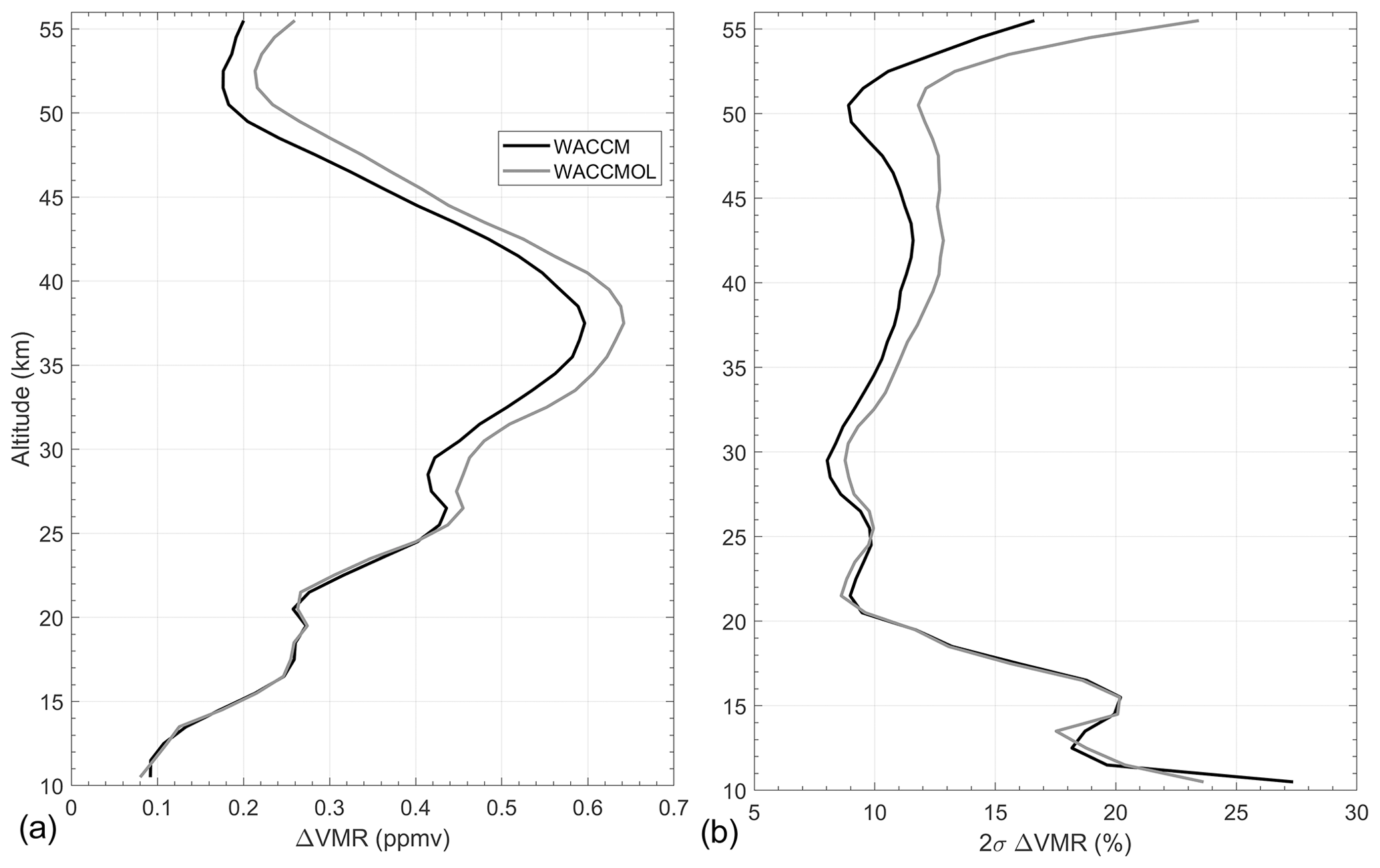
Figure 2Simulated 2σ variability (a) and relative 2σ variability (b) for ACE-FTS–OSIRIS-coincident O3 profiles when interpolating to measurement geolocations from WACCM grid (black) and using WACCMOL (WACCM output at observed locations; grey). Coincidence criteria of within 6 h and 500 km.
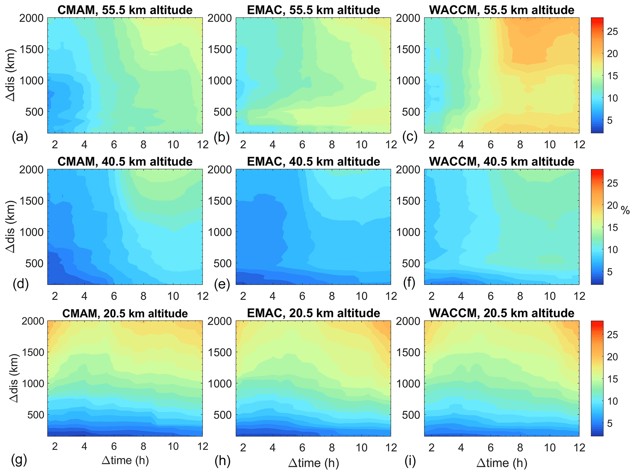
Figure 3Geophysical variability (2σ) between ACE-FTS and OSIRIS O3 derived from the simulated results of CMAM (a, d, g), EMAC (b, e, h), and WACCM (c, f, i), at altitudes of 20.5 km (g–i), 40.5 km (d–f), and 55.5 km (a–c). Calculations performed for time difference criteria of within 1.5 h to within 12 h in 0.5 h increments and distance difference criteria of within 150 km to within 2000 km in 50 km increments.
Simulated geophysical variability can also be determined for a range of coincidence criteria. Figure 3 shows the geophysical variability determined from CMAM, EMAC, and WACCM for all time difference criteria between within 1.5 h and within 12 h in 0.5 h increments and distance difference criteria between within 150 km and within 2000 km in 50 km increments. These were calculated for all three models at all altitude levels (10–56 km), and results are shown for altitude levels of 20.5, 40.5, and 55.5 km.
Again, all three models show very similar geophysical variability patterns for different coincidence criteria. At the lowest altitudes (e.g., 20.5 km), where there are relatively small diurnal variations, for any given distance criterion, geophysical variability tends to stay fairly constant regardless of the time criterion (up to within 12 h). Conversely, for any given time criteria, geophysical variability increases from ∼ 2 %–7 % at within 150 km to ∼ 16 %–23 % at within 2000 km. At the highest altitudes (e.g., 55.5 km), the opposite effect is seen. Since there is a significant diurnal effect, the simulated geophysical variability is fairly consistent at a given time criterion, regardless of the distance criterion; and at any given distance criterion, the geophysical variability typically increases from ∼ 6 %–12 % at within 1 h to 13 %–22 % at within 12 h. At intermediate altitudes (e.g., 40.5 km), where there is a moderate diurnal cycle, the geophysical variability tends to increase with both time and distance criteria. The variability increases from ∼ 2 %–5 % near within 1 h and 100 km to ∼ 12 %–15 % near within 12 h and 2000 km.

Figure 4Ensemble mean geophysical variability (2σ) between ACE-FTS and OSIRIS O3, as estimated from CMAM, EMAC, and WACCM data. Calculations performed for time difference criteria of within 1.5 to 12 h in 0.5 h increments and distance difference criteria of within 150 to 2000 km in 50 km increments. Black circles indicate the coincidence criteria optimized for the greatest number of coincident profiles with geophysical variability limited to 10 %.
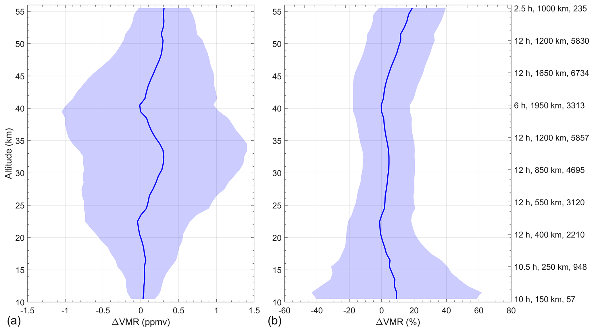
Figure 5Comparisons between ACE-FTS and OSIRIS O3 profile measurements at coincident criteria that, at each altitude, maximize the number of coincident profiles while keeping estimated geophysical variability below 10 %. Solid lines indicate the mean of the differences (a: absolute values; b: relative differences), and shaded regions are the corresponding 2σ variations from the means.
The mean of all three model results was taken to give ensemble mean values of the geophysical variability, shown in Fig. 4. These closely resemble the results described above, with geophysical variability being relatively independent of the time difference criterion at the lower altitude levels, relatively independent of the distance difference criterion at the higher altitude levels, and dependent on both at the intermediate altitude levels. When comparing O3 measurements between ACE-FTS and OSIRIS, these ensemble mean geophysical variability values can be used to optimize coincidence criteria. At each altitude level, “optimized” coincidence criteria can be chosen where there are the greatest number of coincident measured profiles with the estimated geophysical variability less than a desired value. For instance, the circle markers on the plots in Fig. 4 indicate “optimized criteria” where there are the greatest number of coincident ACE-FTS and OSIRIS profiles when the estimated geophysical variability is less than 10 %, and Fig. 5 shows results for comparisons between ACE-FTS and OSIRIS O3 profiles when using the optimized criteria for this chosen 10 % 2σ variability limit at each altitude. It should be noted that in Fig. 5, at some of the altitude levels below 17 km there were no coincidence criteria evaluated where geophysical variability was less than 10 %, and in those cases coincidence criteria of within 1.5 h and 150 km were used. The coincidence criteria can be optimized for any chosen limit of geophysical variability (10 % was chosen in this case), and naturally this could be done for any subset of seasons or latitudes within the collocated data. However, one drawback to having different coincidence criteria at each altitude, especially when making global comparisons, is that it can potentially add biases between altitudes due to changing seasonal and latitudinal sampling. Therefore, care must be taken to ensure that biases of this type are not being introduced.

Figure 6Comparison results between ACE-FTS and OSIRIS O3 for different coincidence criteria: (a) mean of the relative differences, (b) 2σ variation of the relative differences, and (c) number of coincident profiles. Optimized criteria are for less than 10 % geophysical variability above 17 km and less than 15 % below 17 km.
These results can be used not only to constrain the inherent geophysical variability in comparisons between satellite measurements but also to increase the number of usable coincident profiles. Figure 6 shows results of comparisons between ACE-FTS and OSIRIS O3 profiles for five different coincidence criteria: within 2 h and 250 km, within 6 h and 500 km, within 8 h and 1000 km, within 12 h and 2000 km, and criteria optimized at each altitude. The optimized criteria were such that above 17 km the maximum estimated geophysical variability was 10 % and below 17 km it was 15 %. At most altitudes, the bias between the two instruments is relatively independent of coincidence criteria and the profiles exhibit similar variations with altitude. Above 20 km, the differences between the biases given different coincidence criteria are typically on the order of 1 %–4 %. These differences are slightly larger below 20 km, where the maximum difference is 8 % between the 2 h and 250 km criteria and the 12 h and 2000 km criteria. The 2σ standard deviations of the relative differences, shown in Fig. 6b, exhibit greater variability with coincidence criteria. Between 20 and 40 km, the optimized criteria yield standard deviations that are typically better than all the other criteria, with the exception of within 2 h and 250 km below 14 km and between 20 and 42 km. However, with the criteria of 2h and 250 km only 279 coincident profiles (Fig. 5c) are being compared, whereas with the optimized criteria, 1900–5900 profiles are used in the comparisons, leading to a more robust result with a consistent estimate on the geophysical variability uncertainty. The increase in coincident profiles may not be necessary in this exact case where global data are being compared but would be useful in specific regions where there are fewer coincident profiles with which to compare. The greatest improvement to the standard deviations is in the 13–20 km region, where the optimized criteria lead to standard deviations on the same order as the 2 h and 250 km criteria but making use of 2–7 times more profiles and, again, providing an estimate on the geophysical variability uncertainty.
4.2 Hemispheric comparisons
It is also interesting to observe the difference in geophysical variability between the polar Northern Hemisphere (NH; poleward of 50∘ N) region and the polar Southern Hemisphere (SH; poleward of 50∘ S) region, where there is greater O3 variability in general. Figure 7 shows the same plots as those of Fig. 4 but for polar NH and SH data. At 20.5 km, at coincidence criteria of within 8 h and 1000 km, the ensemble mean geophysical variability in the NH is 8 %, whereas in the SH O3 concentrations are estimated to be over twice as variable, at 19 %.
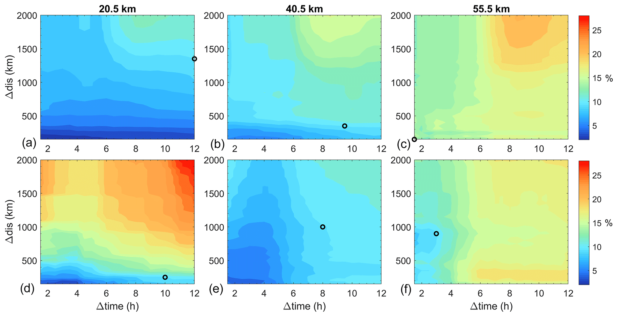
Figure 7Ensemble mean geophysical variability (2σ) between ACE-FTS and OSIRIS O3, as estimated from CMAM, EMAC, and WACCM data: (a–c) for 50–90∘ N and (d–f) for 50–90∘ S. Calculations performed for time difference criteria of within 1.5 h to within 12 h in 0.5 h increments and distance difference criteria of within 150 km to within 2000 km in 50 km increments. Black circles indicate the coincidence criteria optimized for the greatest number of coincident profiles with geophysical variability limited to 10 %.
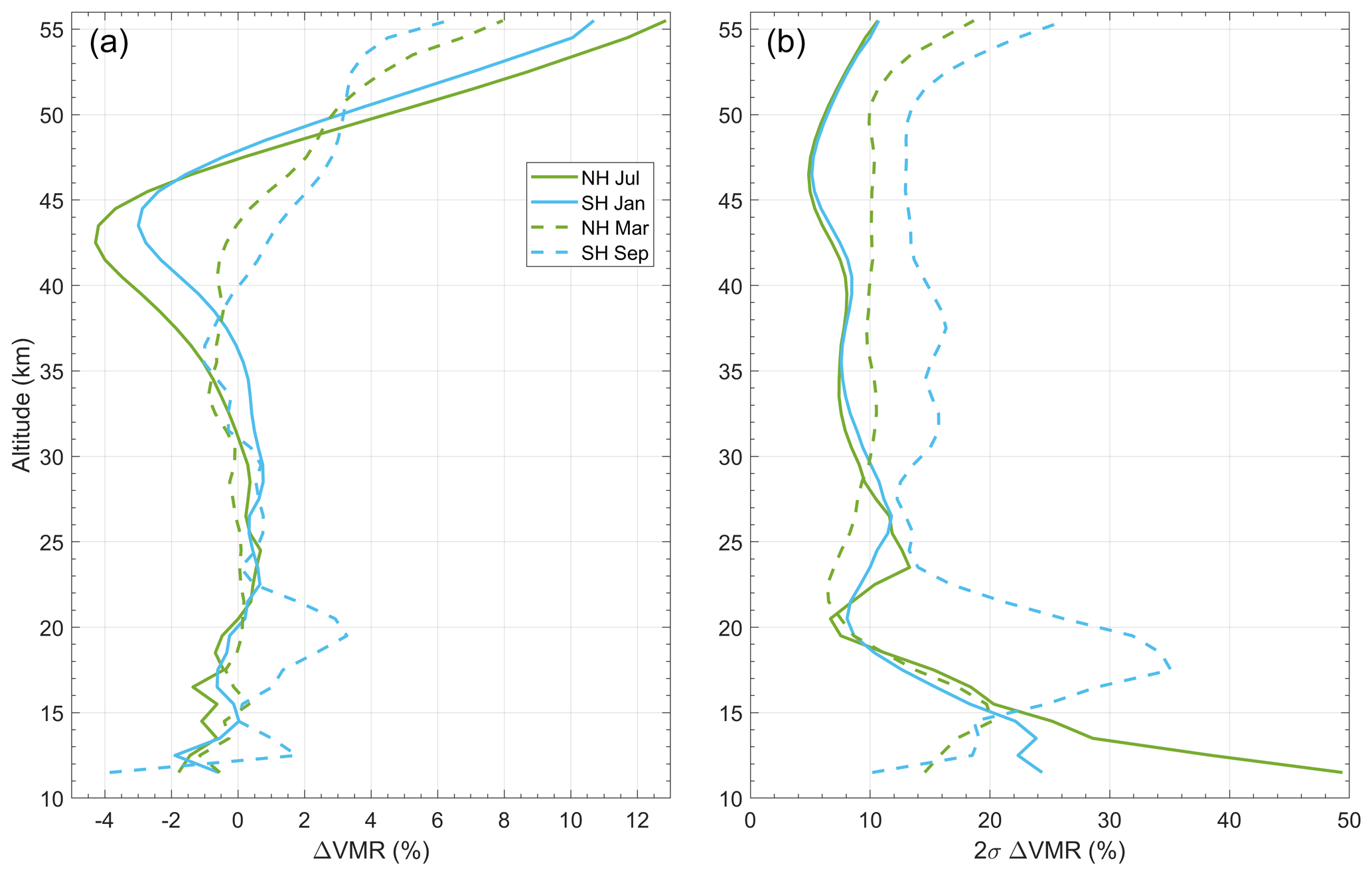
Figure 8Ensemble mean bias (a) and 2σ geophysical variability (b) between ACE-FTS and OSIRIS O3 in the polar regions at coincidence criteria of within 8 h and 1000 km, as estimated from CMAM, EMAC, and WACCM data.
Figure 8 shows the difference in ensemble mean bias and 2σ geophysical variability at coincidence criteria of 8 h and 1000 km binned by hemisphere and month. It shows that, unsurprisingly, there is a much larger difference between polar NH and SH in the stratosphere during the end of winter than at the beginning of summer. This is due to the stronger southern polar vortex.
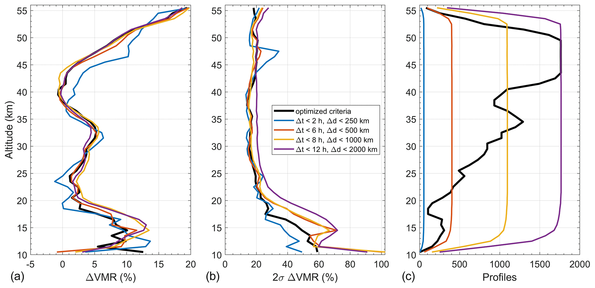
Figure 9The bias (a) and 2σ variability (b) of the relative differences between ACE-FTS and OSIRIS O3 profiles in the southern polar region at different coincidence criteria, including the optimized criteria for 10 % variability above 17 km and 15 % below 17 km and the corresponding number of coincident profiles (c).
Above 15 km in the summer months, when there is not a strong polar vortex, the NH and SH exhibit similar geophysical variability profiles, with variability on the order of 5 %–15 %. In the same altitude region in the SH spring, geophysical variability is much larger, due to the strong and prevalent southern polar vortex, which is just starting to break up with the onset of sunlight; and at laxer coincidence criteria, it is more likely that one instrument will be observing inside the southern polar vortex and the other outside the vortex, which can have different atmospheric conditions. The variability is on the order of 15 %–20 % above 22 km and peaks at 35 % near 18 km, where there is some of the most ozone depletion. As can be seen in Fig. 7a and d, in the lower stratosphere in the polar SH, the geophysical variability is more sensitive to the time coincidence criterion than in the polar NH. The NH geophysical variability above 30 km is also greater at the end of winter (∼ 5 %–10 %) than during the summer (∼ 10 %–15 %). This could be due to stronger planetary wave forcing in the NH (e.g., Butchart, 2014; de la Cámara et al., 2018) and/or stronger descent of NO and NO2 following sudden stratospheric warming events (e.g., Reddmann et al., 2010).
Figure 9 shows the estimated bias and the mean 2σ variability of the relative differences between ACE-FTS and OSIRIS O3 profiles in the polar SH for different coincidence criteria, including the optimized criteria for 10 % geophysical variability above 17 km and 15 % below 17 km. As with the global comparisons, the bias is largely unaffected by the choice of coincidence criteria. Between 20 and 42 km, all the coincidence criteria lead to similar variability profiles on the order of 15 %–20 %. Below 20 km, the optimized criteria tend to yield better variability results than the criteria of within 6 h and greater; however, they yield larger values than the 2 h and 250 km criteria. The benefits of the optimized criteria case in this region are that there is a consistent estimate of the geophysical variability and that it makes use of more coincident profiles – the 2 h and 250 km criteria have a maximum of only 54 profiles, whereas the optimized criteria make use of up to 307 profiles near 15 km.
This study used three different chemistry–climate models – CMAM, EMAC, and WACCM – that were run in specified-dynamics mode; i.e., meteorological fields were nudged towards observational data. The O3 data from these models were sampled at ACE-FTS and OSIRIS times and locations in order to estimate the geophysical variation (as characterized by the 2σ standard deviation of differences) inherent in the satellite O3 comparisons at varying coincidence criteria. The averages of the simulated values were taken in order to obtain ensemble mean values of the geophysical variation. Based on the differences in the estimated geophysical variation between WACCM and WACCMOL (WACCM output at observed locations), the interpolation method used in this study yields the most accurate results in the lower to mid-stratosphere, up to ∼ 25 km. Above 30 km the interpolation may lead to an underestimation of the geophysical variability on the order of 0.04–0.06 ppmv (a relative difference of up to 23 %).
When analyzing the global data, all three models show similar geophysical variability patterns based on coincidence criteria. In the lower stratosphere, the geophysical variation is, within the criteria limits, relatively independent of the time criterion and increases as the distance criterion is widened. In the upper stratosphere, where there is a stronger O3 diurnal cycle, the geophysical variation tends to be independent of the distance criterion and increases when the time criterion is increased. In the middle stratosphere, the geophysical variation tends to increase with increasing time and distance criteria. Ensemble mean values in the lower stratosphere show that geophysical variability is much larger in the high-latitude SH than in the high-latitude NH, except at very tight criteria (e.g., within 2 h and 200 km). This is due to the more consistent presence of the southern polar vortex, which often leads to coincident ACE-FTS and OSIRIS measurements sampling two different air masses (inside and outside the vortex). On average in the NH, geophysical variation decreases more strongly with altitude from 24 % at 12 km to 8 % at 20 km, whereas in the SH, geophysical variation is 28 % at 17 km and 20 % at 20 km. Also, in the polar SH in the lower stratosphere, geophysical variability does not tend to be time independent.
When comparing profiles from satellite data, the ensemble means of the simulated geophysical variability can be used to optimize the chosen coincidence criteria, allowing for a large number of coincident profiles while limiting the estimated variability to a desired quantity (on the scale of the measurement uncertainties). This method allows for relatively simple, consistent estimates of geophysical variability inherent in the comparison results and allows for making use of more coincident profiles, which is an advantage for solar occultation instruments that tend to have fewer observation profiles than sensors using other limb-viewing techniques. However, this does lead to different measurement times or locations being compared at different altitude levels and therefore care must be taken such that it does not lead to regional and/or seasonal sampling differences in the profiles of the comparison results, which could add spurious features. This technique of using the natural variability estimates in order to optimize the coincidence criteria can, however, also be used for data that are isolated to a single season or latitude range.
The sampled data sets and simulations used for these analyses are available (https://doi.org/10.5683/SP2/ZHGQOI, Sheese et al., 2020). The ACE-FTS Level 2 data can be obtained via the ACE-FTS website (registration required): http://www.ace.uwaterloo.ca (last access: 21 January 2021). The OSIRIS data can be obtained via http://odin-osiris.usask.ca (registration required, last access: 21 January 2021; https://doi.org/10.5281/zenodo.4110053, Roth, 2020). The CMAM30 data set can be downloaded via Environment and Climate Change Canada's climate modelling website: https://climate-modelling.canada.ca/climatemodeldata/cmam/output/CMAM/CMAM30-SD/ (CCCma, 2021).
The study was designed by PES, TvC, and KAW. PES wrote the paper. PES performed the analyses with contributions from FK. Satellite data used in this study were provided by CDB and DAD. Model simulations used in the study were provided by DP, DEK, and PJ. Valuable comments on the paper were provided by KAW, CDB, FK, DAD, DP, DEK, PJ, and TvC.
Thomas von Clarmann is associate editor of AMT but he has not been involved in the evaluation of this paper.
This article is part of the special issue “Towards Unified Error Reporting (TUNER)”. It is not associated with a conference.
This project was funded by the Canadian Space Agency (CSA). The Atmospheric Chemistry Experiment is a Canadian-led mission mainly supported by the CSA. We thank Peter Bernath for his leadership of the ACE mission. Odin is a Swedish-led satellite project funded jointly by Sweden (Swedish National Space Board), Canada (CSA), France (Centre National d'Études Spatiales), and Finland (Tekes), with support by the third-party mission programme of the European Space Agency (ESA). The ACE-FTS height-dependent latitudes and longitudes were obtained from the geolocation files on the ACE-FTS website (http://databace.scisat.ca, last access: 21 January 2021; registration required); the ACE-FTS level 2 O3 data were also obtained from that site. The OSIRIS level 1 height-dependent times, latitudes, and longitudes were obtained from the OSIRIS website (http://odin-osiris.usask.ca), as were the level 2 O3 data. We thank the CSA for financial support that made the development of the CMAM30 data set possible. The CMAM30 data set can be downloaded from http://climate-modelling.canada.ca/climatemodeldata/cmam/cmam30/index.shtml. The EMAC simulations have been performed at the German Climate Computing Centre (DKRZ) through support from the Bundesministerium für Bildung und Forschung (BMBF). DKRZ and its scientific steering committee are gratefully acknowledged for providing the HPC and data archiving resources for this consortial project ESCiMo (Earth System Chemistry integrated Modelling). WACCM is a component of the Community Earth System Model (CESM), which is supported by the National Science Foundation. We would like to acknowledge high-performance computing support from Cheyenne (https://doi.org/10.5065/D6RX99HX, last access: 21 January 2021) provided by NCAR's Computational and Information Systems Laboratory, sponsored by the National Science Foundation. We thank NASA Goddard Space Flight Center for the MERRA data (available freely online at http://disc.sci.gsfc.nasa.gov, last access: 21 January 2021).
This research has been supported by the Canadian Space Agency (contract no. 9F045-180034/001/MTB).
This paper was edited by Nathaniel Livesey and reviewed by two anonymous referees.
Adams, C., Bourassa, A. E., Bathgate, A. F., McLinden, C. A., Lloyd, N. D., Roth, C. Z., Llewellyn, E. J., Zawodny, J. M., Flittner, D. E., Manney, G. L., Daffer, W. H., and Degenstein, D. A.: Characterization of Odin-OSIRIS ozone profiles with the SAGE II dataset, Atmos. Meas. Tech., 6, 1447–1459, https://doi.org/10.5194/amt-6-1447-2013, 2013.
Aghedo, A. M., Bowman, K. W., Shindell, D. T., and Faluvegi, G.: The impact of orbital sampling, monthly averaging and vertical resolution on climate chemistry model evaluation with satellite observations, Atmos. Chem. Phys., 11, 6493–6514, https://doi.org/10.5194/acp-11-6493-2011, 2011.
Bacmeister, J. T., Kuell, V., Offermann, D., Riese, M., and Elkins, J. W.: Intercomparison of satellite and aircraft observations of ozone, CFC-11 and NOy using trajectory mapping, J. Geophys. Res., 104, 16379–16390, https://doi.org/10.1029/1999JD900173, 1999.
Bernath, P. F., McElroy, C. T., Abrams, M. C., Boone, C. D., Butler, M., Camy-Peyret, C., Carleer, M., Clerbaux, C., Coheur, P.-F., Colin, R., DeCola, P., DeMazière, M., Drummond, J. R., Dufour, D., Evans, W. F. J., Fast, H., Fussen, D., Gilbert, K., Jennings, D. E., Llewellyn, E. J., Lowe, R. P., Mahieu, E., McConnell, J. C., McHugh, M., McLeod, S. D., Michaud, R., Midwinter, C., Nassar, R., Nichitiu, F., Nowlan, C., Rinsland, C. P., Rochon, Y. J., Rowlands, N., Semeniuk, K., Simon, P., Skelton, R., Sloan, J. J., Soucy, M.-A., Strong, K., Tremblay, P., Turnbull, D., Walker, K. A., Walkty, I., Wardle, D. A., Wehrle, V., Zander, R., and Zou, J.: Atmospheric Chemistry Experiment (ACE): Mission overview, Geophys. Res. Lett., 32, L15S01, https://doi.org/10.1029/2005GL022386, 2005.
Boone, C. D., Nassar, R., Walker, K. A., Rochon, Y., McLeod, S. D., Rinsland, C. P., and Bernath, P. F.: Retrievals for the Atmospheric Chemistry Experiment Fourier-Transform Spectrometer, Appl. Optics, 44, 7218–7231, https://doi.org/10.1364/AO.44.007218, 2005.
Boone, C. D., Walker, K. A., and Bernath, P. F.: Version 3 Retrievals for the Atmospheric Chemistry Experiment Fourier Transform Spectrometer (ACE-FTS), The Atmospheric Chemistry Experiment ACE at 10: A Solar Occultation Anthology, A. Deepak Publishing, Hampton, Virginia, USA, 103–127, 2013.
Bourassa, A. E., McLinden, C. A., Bathgate, A. F., Elash, B. J., and Degenstein, D. A.: Precision estimate for Odin-OSIRIS limb scatter retrievals, J. Geophys. Res., 117, D04303, https://doi.org/10.1029/2011JD016976, 2012.
Bourassa, A. E., Roth, C. Z., Zawada, D. J., Rieger, L. A., McLinden, C. A., and Degenstein, D. A.: Drift-corrected Odin-OSIRIS ozone product: algorithm and updated stratospheric ozone trends, Atmos. Meas. Tech., 11, 489–498, https://doi.org/10.5194/amt-11-489-2018, 2018.
Brakebusch, M., Randall, C. E., Kinnison, D. E., Tilmes, S., Santee, M. L., and Manney, G. L.: Evaluation of Whole Atmosphere Community Climate Model simulations of ozone during Arctic winter 2004–2005, J. Geophys. Res.-Atmos., 118, 2673–2688, https://doi.org/10.1002/jgrd.50226, 2013.
Butchart, N.: The Brewer-Dobson circulation, Rev. Geophys., 52, 157–184, https://doi.org/10.1002/2013RG000448, 2014.
Canadian Centre for Climate Modelling and Analysis (CCCma): CMAM30 Data, available at: https://climate-modelling.canada.ca/climatemodeldata/cmam/output/CMAM/CMAM30-SD/, last access: 21 January 2021.
Chandran, A., Collins, R., and Harvey, V.: Stratosphere-mesosphere coupling during stratospheric sudden warming events, Adv. Space Res., 53, 1265–1289, https://doi.org/10.1016/j.asr.2014.02.005, 2014.
Danilin, M. Y., Santee, M. L., Rodriguez, J. M., Ko, M. K. W., Mergenthaler, J. M., Kumer, J. B., Tabazadeh, A., and Livesey, N. J.: Trajectory hunting: a case study of rapid chlorine activation in December 1992 as seen by UARS, J. Geophys. Res., 105, 4003–4018, https://doi.org/10.1029/1999JD901054, 2000.
Danilin, M. Y., Ko, M. K. W., Froidevaux, L., Santee, M. L., Lyjak, L. V., Bevilacqua, R. M., Zawodny, J. M., Sasano, Y., Irie, H., Kondo, Y., Russell, J. M., Scott, C. J., and Read, W. G.: Trajectory hunting as an effective technique to validate multiplatform measurements: analysis of the MLS, HALOE, SAGE-II, ILAS, and POAM-II data in October–November 1996, J. Geophys. Res., 107, 4420, https://doi.org/10.1029/2001JD002012, 2002a.
Danilin, M. Y., Ko, K. W., Bevilacqua, R. M., Lyjak, L. V., Froidevaux, L., Santee, M. L., Zawodny, J. M., Hoppel, K. W., Richard, E. C., Spackman, J. R., Weinstock, E. M., Herman, R. L., McKinney, K. A., Wennberg, P. O., Eisele, F. L., Stimpfle, R. M., Scott, C. J., Elkins, J. W., and Bui, T. V.: Comparison of ER-2 aircraft and POAM III, MLS, and SAGE II satellite measurements during SOLVE using traditional correlative analysis and trajectory hunting technique, J. Geophys. Res., 107, 8315, https://doi.org/10.1029/2001JD000781, 2002b.
Dee, D. P., Uppala, S. M., Simmons, A. J., Berrisford, P., Poli, P., Kobayashi, S., Andrae, U., Balmaseda, M. A., Balsamo, G., Bauer, P., Bechtold, P., Beljaars, A. C. M., van de Berg, L., Bidlot, J., Bormann, N., Delsol, C., Dragani, R., Fuentes, M., Geer, A. J., Haimberger, L., Healy, S. B., Hersbach, H., Hólm, E. V., Isaksen, L., Kållberg, P., Köhler, M., Matricardi, M., McNally, A. P., Monge-Sanz, B. M., Morcrette, J.-J., Park, B.- K., Peubey, C., de Rosnay, P., Tavolato, C., Thépaut, J.-N., and Vitart, F.: The ERA-Interim reanalysis: configuration and performance of the data assimilation system, Q. J. Roy. Meteor. Soc., 137, 553–597, https://doi.org/10.1002/qj.828, 2011.
Degenstein, D. A., Bourassa, A. E., Roth, C. Z., and Llewellyn, E. J.: Limb scatter ozone retrieval from 10 to 60 km using a multiplicative algebraic reconstruction technique, Atmos. Chem. Phys., 9, 6521–6529, https://doi.org/10.5194/acp-9-6521-2009, 2009.
de Grandpré, J., Beagley, S. R., Fomichev, V. I., Griffioen, E., McConnell, J. C., Medvedev, A. S., and Shepherd, T. G.: Ozone climatology using interactive chemistry: results from the Canadian Middle Atmosphere Model, J. Geophys. Res., 105, 26475–26492, https://doi.org/10.1029/2000JD900427, 2000.
de la Cámara, A., Abalos, M., and Hitchcock, P.: Changes in stratospheric transport and mixing during sudden stratospheric warmings. J. Geophys. Res., 123, 3356–3373, https://doi.org/10.1002/2017JD028007, 2018.
Dupuy, E., Walker, K. A., Kar, J., Boone, C. D., McElroy, C. T., Bernath, P. F., Drummond, J. R., Skelton, R., McLeod, S. D., Hughes, R. C., Nowlan, C. R., Dufour, D. G., Zou, J., Nichitiu, F., Strong, K., Baron, P., Bevilacqua, R. M., Blumenstock, T., Bodeker, G. E., Borsdorff, T., Bourassa, A. E., Bovensmann, H., Boyd, I. S., Bracher, A., Brogniez, C., Burrows, J. P., Catoire, V., Ceccherini, S., Chabrillat, S., Christensen, T., Coffey, M. T., Cortesi, U., Davies, J., De Clercq, C., Degenstein, D. A., De Mazière, M., Demoulin, P., Dodion, J., Firanski, B., Fischer, H., Forbes, G., Froidevaux, L., Fussen, D., Gerard, P., Godin-Beekmann, S., Goutail, F., Granville, J., Griffith, D., Haley, C. S., Hannigan, J. W., Höpfner, M., Jin, J. J., Jones, A., Jones, N. B., Jucks, K., Kagawa, A., Kasai, Y., Kerzenmacher, T. E., Kleinböhl, A., Klekociuk, A. R., Kramer, I., Küllmann, H., Kuttippurath, J., Kyrölä, E., Lambert, J.-C., Livesey, N. J., Llewellyn, E. J., Lloyd, N. D., Mahieu, E., Manney, G. L., Marshall, B. T., McConnell, J. C., McCormick, M. P., McDermid, I. S., McHugh, M., McLinden, C. A., Mellqvist, J., Mizutani, K., Murayama, Y., Murtagh, D. P., Oelhaf, H., Parrish, A., Petelina, S. V., Piccolo, C., Pommereau, J.-P., Randall, C. E., Robert, C., Roth, C., Schneider, M., Senten, C., Steck, T., Strandberg, A., Strawbridge, K. B., Sussmann, R., Swart, D. P. J., Tarasick, D. W., Taylor, J. R., Tétard, C., Thomason, L. W., Thompson, A. M., Tully, M. B., Urban, J., Vanhellemont, F., Vigouroux, C., von Clarmann, T., von der Gathen, P., von Savigny, C., Waters, J. W., Witte, J. C., Wolff, M., and Zawodny, J. M.: Validation of ozone measurements from the Atmospheric Chemistry Experiment (ACE), Atmos. Chem. Phys., 9, 287–343, https://doi.org/10.5194/acp-9-287-2009, 2009.
Fassò, A., Ignaccolo, R., Madonna, F., Demoz, B. B., and Franco-Villoria, M.: Statistical modelling of collocation uncertainty in atmospheric thermodynamic profiles, Atmos. Meas. Tech., 7, 1803–1816, https://doi.org/10.5194/amt-7-1803-2014, 2014.
Froidevaux, L., Kinnison, D. E., Wang, R., Anderson, J., and Fuller, R. A.: Evaluation of CESM1 (WACCM) free-running and specified dynamics atmospheric composition simulations using global multispecies satellite data records, Atmos. Chem. Phys., 19, 4783–4821, https://doi.org/10.5194/acp-19-4783-2019, 2019.
Gillett, N. P., Scinocca, J. F., Plummer, D. A., and Reader, M. C.: Sensitivity of climate to dynamically-consistent zonal asymmetries in ozone, Geophys. Res. Lett., 36, L10809, https://doi.org/10.1029/2009GL037246, 2009.
Guan, B., Waliser, D. E., Li, J.-L. F., and da Silva, A.: Evaluating the impact of orbital sampling on satellite–climate model comparisons, J. Geophys. Res.-Atmos., 118, 1–15, https://doi.org/10.1029/2012JD018590, 2013.
Hubert, D., Lambert, J.-C., Verhoelst, T., Granville, J., Keppens, A., Baray, J.-L., Bourassa, A. E., Cortesi, U., Degenstein, D. A., Froidevaux, L., Godin-Beekmann, S., Hoppel, K. W., Johnson, B. J., Kyrölä, E., Leblanc, T., Lichtenberg, G., Marchand, M., McElroy, C. T., Murtagh, D., Nakane, H., Portafaix, T., Querel, R., Russell III, J. M., Salvador, J., Smit, H. G. J., Stebel, K., Steinbrecht, W., Strawbridge, K. B., Stübi, R., Swart, D. P. J., Taha, G., Tarasick, D. W., Thompson, A. M., Urban, J., van Gijsel, J. A. E., Van Malderen, R., von der Gathen, P., Walker, K. A., Wolfram, E., and Zawodny, J. M.: Ground-based assessment of the bias and long-term stability of 14 limb and occultation ozone profile data records, Atmos. Meas. Tech., 9, 2497–2534, https://doi.org/10.5194/amt-9-2497-2016, 2016.
Jöckel, P., Kerkweg, A., Pozzer, A., Sander, R., Tost, H., Riede, H., Baumgaertner, A., Gromov, S., and Kern, B.: Development cycle 2 of the Modular Earth Submodel System (MESSy2), Geosci. Model Dev., 3, 717–752, https://doi.org/10.5194/gmd-3-717-2010, 2010.
Jöckel, P., Tost, H., Pozzer, A., Kunze, M., Kirner, O., Brenninkmeijer, C. A. M., Brinkop, S., Cai, D. S., Dyroff, C., Eckstein, J., Frank, F., Garny, H., Gottschaldt, K.-D., Graf, P., Grewe, V., Kerkweg, A., Kern, B., Matthes, S., Mertens, M., Meul, S., Neumaier, M., Nützel, M., Oberländer-Hayn, S., Ruhnke, R., Runde, T., Sander, R., Scharffe, D., and Zahn, A.: Earth System Chemistry integrated Modelling (ESCiMo) with the Modular Earth Submodel System (MESSy) version 2.51, Geosci. Model Dev., 9, 1153–1200, https://doi.org/10.5194/gmd-9-1153-2016, 2016.
Jonsson, A. I., de Grandpré, J., Fomichev, V. I., McConnell, J. C., and Beagley, S. R.: Doubled CO2-induced cooling in the middle atmosphere: Photochemical analysis of the ozone radiative feedback, J. Geophys. Res., 109, D24103, https://doi.org/10.1029/2004JD005093, 2004.
Khosrawi, F., Kirner, O., Sinnhuber, B.-M., Johansson, S., Höpfner, M., Santee, M. L., Froidevaux, L., Ungermann, J., Ruhnke, R., Woiwode, W., Oelhaf, H., and Braesicke, P.: Denitrification, dehydration and ozone loss during the 2015/2016 Arctic winter, Atmos. Chem. Phys., 17, 12893–12910, https://doi.org/10.5194/acp-17-12893-2017, 2017.
Kolonjari, F., Plummer, D. A., Walker, K. A., Boone, C. D., Elkins, J. W., Hegglin, M. I., Manney, G. L., Moore, F. L., Pendlebury, D., Ray, E. A., Rosenlof, K. H., and Stiller, G. P.: Assessing stratospheric transport in the CMAM30 simulations using ACE-FTS measurements, Atmos. Chem. Phys., 18, 6801–6828, https://doi.org/10.5194/acp-18-6801-2018, 2018.
Liu, J., Tarasick, D. W., Fioletov, V. E., McLinden, C., Zhao, T., Gong, S., Sioris, C., Jin, J. J., Liu, G., and Moeini, O.: A global ozone climatology from ozone soundings via trajectory mapping: a stratospheric perspective, Atmos. Chem. Phys., 13, 11441–11464, https://doi.org/10.5194/acp-13-11441-2013, 2013.
Llewellyn, E. J., Lloyd, N. D., Degenstein, D. A., Gattinger, R. L., Petelina, S. V., Bourassa, A. E., Wiensz, J. T., Ivanov, E. V., McDade, I. C., Solheim, B. H., McConnell, J. C., Haley, C. S., von Savigny, C., Sioris, C. E., McLinden, C. A., Griffioen, E., Kaminski, J., Evans, W. F. J., Puckrin, E., Strong, K., Wehrle, V., Hum, R. H., Kendall, D. J. W., Matsushita, J., Murtagh, D. P., Brohede, S., Stegman, J., Witt, G., Barnes, G., Payne, W. F., Piché, L., Smith, K., Warshaw, G., Deslauniers, D. L., Marchand, P., Richardson, E. H., King, R.A., Wevers, I., McCreath, W., Kyrola, E., Oikarinen, L., Leppelmeier, G. W., Auvinen, H., Mégie, G., Hauchecorne, A., Lefèvre, F., de La Nöe, J., Ricaud, P., Frisk, U., Sjoberg, F., von Schéele, F., and Nordh, L.: The OSIRIS instrument on the Odin spacecraft, Can. J. Phys., 82, 411–422, https://doi.org/10.1139/P04-005, 2004.
Loew, A., Bell, W., Brocca, L., Bulgin, C. E., Burdanowitz, J., Calbet, X., Donner, R. V., Ghent, D., Gruber, A., Kaminski, T., Kinzil, J., Klepp, C., Lambert, J.-C., Schaepman-Strub, G., Schröder, M., and Verhoelst, T.: Validation practices for satellite-based Earth observation data across communities, Rev. Geophys., 55, 779–817, https://doi.org/10.1002/2017RG000562, 2017.
Marsh, D. R., Mills, M. J., Kinnison, D. E., Lamarque, J.-F., Calvo, N., and Polvani, L. M.: Climate change from 1850 to 2005 simulated in CESM1(WACCM), J. Climate, 26, 7372–7391, https://doi.org/10.1175/JCLI-D-12-00558.1, 2013.
McLandress, C., Shepherd, T. G., Scinocca, J. F., Plummer, D. A., Sigmond, M., Jonsson, A. I., and Reader, M. C.: Separating the Dynamical Effects of Climate Change and Ozone Depletion. Part II: Southern Hemisphere Troposphere. J. Climate, 24, 1850–1868, https://doi.org/10.1175/2010JCLI3958.1, 2011.
McLandress, C., Scinocca, J. F., Shepherd, T. G., Reader, M. C., and Manney, G. L.: Dynamical control of the mesosphere by orographic and nonorographic gravity wave drag during the extended northern winters of 2006 and 2009, J. Atmos. Sci., 70, 2152–2169, https://doi.org/10.1175/JAS-D-12-0297.1, 2013.
Merkel, A. W., Harder, J. W., Marsh, D. R., Smith, A. K., Fontenla, J. M., and Woods, T. N.: The impact of solar spectral irradiance variability on middle atmospheric ozone, Geophys. Res. Lett., 38, L13802, https://doi.org/10.1029/2011GL047561, 2011.
Meul, S., Langematz, U., Oberländer, S., Garny, H., and Jöckel, P.: Chemical contribution to future tropical ozone change in the lower stratosphere, Atmos. Chem. Phys., 14, 2959–2971, https://doi.org/10.5194/acp-14-2959-2014, 2014.
Millán, L. F., Livesey, N. J., Santee, M. L., Neu, J. L., Manney, G. L., and Fuller, R. A.: Case studies of the impact of orbital sampling on stratospheric trend detection and derivation of tropical vertical velocities: solar occultation vs. limb emission sounding, Atmos. Chem. Phys., 16, 11521–11534, https://doi.org/10.5194/acp-16-11521-2016, 2016.
Morgenstern, O., Hegglin, M. I., Rozanov, E., O'Connor, F. M., Abraham, N. L., Akiyoshi, H., Archibald, A. T., Bekki, S., Butchart, N., Chipperfield, M. P., Deushi, M., Dhomse, S. S., Garcia, R. R., Hardiman, S. C., Horowitz, L. W., Jöckel, P., Josse, B., Kinnison, D., Lin, M., Mancini, E., Manyin, M. E., Marchand, M., Marécal, V., Michou, M., Oman, L. D., Pitari, G., Plummer, D. A., Revell, L. E., Saint-Martin, D., Schofield, R., Stenke, A., Stone, K., Sudo, K., Tanaka, T. Y., Tilmes, S., Yamashita, Y., Yoshida, K., and Zeng, G.: Review of the global models used within phase 1 of the Chemistry–Climate Model Initiative (CCMI), Geosci. Model Dev., 10, 639–671, https://doi.org/10.5194/gmd-10-639-2017, 2017.
Morris, G. A., Schoeberl, M. R., Sparling, L. C., Newman, P. A., Lait, L. R., Elson, L., Walters, J., Suttie, R. A., Roche, A., Kumer, J., and Russel, J. M.: Trajectory mapping and applications to data from the Upper Atmosphere Research Satellite, J. Geophys. Res., 100, 16491–16505, https://doi.org/10.1029/95JD01072, 1995.
Morris, G. A., Gleason, J. F., Ziemke, J., and Schoeberl, M. R.: Trajectory mapping: A tool for validation of trace gas observations, J. Geophys. Res., 105, 17875–17894, https://doi.org/10.1029/1999JD901118, 2000.
Reddmann, T., Ruhnke, R., Versick, S., and Kouker, W.: Modeling disturbed stratospheric chemistry during solar-induced NOx enhancements observed with MIPAS/ENVISAT, J. Geophys. Res., 115, D00I11, https://doi.org/10.1029/2009JD012569, 2010.
Rienecker, M. M., Suarez, M. J., Gelaro, R., Todling, R., Bacmeister, J., Liu, E., Bosilovich, M. G., Schubert, S. D., Takacs, L., Kim, G.-K., Bloom, S., Chen, J., Collins, D., Conaty, A., da Silva, A., Gu, W., Joiner, J., Koster, R. D., Lucchesi, R., Molod, A., Owens, T., Pawson, S., Pegion, P., Redder, C. R., Reichle, R., Robertson, F. R., Ruddick, A. G., Sienkiewicz, M., and Woollen, J.: MERRA: NASA's Modern-Era Retrospective Analysis for Research and Applications, J. Climate, 24, 3624–3648, https://doi.org/10.1175/JCLI-D-11-00015.1, 2011.
Roth, C. Z.: OSIRIS Ozone v5.07 (Version 5.07) [Data set], Zenodo, https://doi.org/10.5281/zenodo.4110053, 2020.
Roth, C. Z., Degenstein, D. A., Bourassa, A. E., and Llewellyn, E.J.: The retrieval of vertical profiles of the ozone number density using Chappuis band absorption information and a multiplicative algebraic reconstruction technique, Can. J. Phys., 85, 1225–1243, https://doi.org/10.1139/P07-130, 2007.
Rothman, L. S., Jacquemart, D., Barbe, A., Chris Benner, D., Birk, M., Browne, L. R., Carleer, M. R., Chackerian Jr, C., Chance, K., Coudert, L. H., Dana, V., Devi, V. M., Flaud, J. -M., Gamache, R. R., Goldman, A., Hartmann, J. -M., Jucks, K. W., Maki, A. G., Mandin, J. -Y., Massien, S. T., Orphal, J., Perrin, A., Rinsland, C. P., Smith, M. A. H., Tennyson, J., Tolchenov, R. N., Toth, R. A., Vander Auwera, J., Varanasiq, P., and Wagner, G.: The HITRAN 2004 molecular spectroscopic database, J. Quant. Spectrosc. Ra., 96, 139–204, https://doi.org/10.1016/j.jqsrt.2004.10.008, 2005.
Sakazaki, T., Shiotani, M., Suzuki, M., Kinnison, D., Zawodny, J. M., McHugh, M., and Walker, K. A.: Sunset–sunrise difference in solar occultation ozone measurements (SAGE II, HALOE, and ACE–FTS) and its relationship to tidal vertical winds, Atmos. Chem. Phys., 15, 829–843, https://doi.org/10.5194/acp-15-829-2015, 2015.
Scinocca, J. F., McFarlane, N. A., Lazare, M., Li, J., and Plummer, D.: Technical Note: The CCCma third generation AGCM and its extension into the middle atmosphere, Atmos. Chem. Phys., 8, 7055–7074, https://doi.org/10.5194/acp-8-7055-2008, 2008.
Sheese, P. E., Boone, C. D., and Walker, K. A.: Detecting physically unrealistic outliers in ACE-FTS atmospheric measurements, Atmos. Meas. Tech., 8, 741–750, https://doi.org/10.5194/amt-8-741-2015, 2015.
Sheese, P. E., Walker, K. A., Boone, C. D., McLinden, C. A., Bernath, P. F., Bourassa, A. E., Burrows, J. P., Degenstein, D. A., Funke, B., Fussen, D., Manney, G. L., McElroy, C. T., Murtagh, D., Randall, C. E., Raspollini, P., Rozanov, A., Russell III, J. M., Suzuki, M., Shiotani, M., Urban, J., von Clarmann, T., and Zawodny, J. M.: Validation of ACE-FTS version 3.5 NOy species profiles using correlative satellite measurements, Atmos. Meas. Tech., 9, 5781–5810, https://doi.org/10.5194/amt-9-5781-2016, 2016.
Sheese, P. E., Walker, K. A., Boone, C. D., Bernath, P. F., Froidevaux, L., Funke, B., Raspollini, P., and von Clarmann, T.: ACE-FTS ozone, water vapour, nitrous oxide, nitric acid, and carbon monoxide profile comparisons with MIPAS and MLS, J. Quant. Spectrosc. Ra., 186, 63–80, https://doi.org/10.1016/j.jqsrt.2016.06.026, 2017.
Sheese, P. E., Walker, K. A., Boone, C. D., Degenstein, D. A., Kolonjari, F., Plummer, D., Kinnison, D. E., Jöckel, P., and von Clarmann, T.: Data sets and simulations used for Model estimations of geophysical variability between satellite measurements of ozone profiles, Scholars Portal Dataverse, V2, https://doi.org/10.5683/SP2/ZHGQOI, 2020.
Sofieva, V. F., Kalakoski, N., Päivärinta, S.-M., Tamminen, J., Laine, M., and Froidevaux, L.: On sampling uncertainty of satellite ozone profile measurements, Atmos. Meas. Tech., 7, 1891–1900, https://doi.org/10.5194/amt-7-1891-2014, 2014.
SPARC: SPARC CCMVal Report on the Evaluation of Chemistry-Climate Models, edited by: Eyring, V., Shepherd, T., and Waugh, D., SPARC Report No. 5, WCRP-30/2010, WMO/TD – No. 40, available at: http://www.sparc-climate.org/publications/sparc-reports/ (last access: 21 January 2021), 2010.
Toohey, M., Hegglin, M. I., Tegtmeier, S., Anderson, J., Añel, J. A., Bourassa, A., Brohede, S., Degenstein, D., Froidevaux, L., Fuller, R., Funke, B., Gille, J., Jones, A., Kasai, Y., Krüger, K., Kyrölä, E., Neu, J. L., Rozanov, A., Smith, L., Urban, J., von Clarmann, T., Walker, K. A., and Wang, R. H. J.: Characterizing sampling biases in the trace gas climatologies of the SPARC Data Initiative, J. Geophys. Res.-Atmos., 118, 11847–11862, https://doi.org/10.1002/jgrd.50874, 2013.
Verhoelst, T., Granville, J., Hendrick, F., Köhler, U., Lerot, C., Pommereau, J.-P., Redondas, A., Van Roozendael, M., and Lambert, J.-C.: Metrology of ground-based satellite validation: co-location mismatch and smoothing issues of total ozone comparisons, Atmos. Meas. Tech., 8, 5039–5062, https://doi.org/10.5194/amt-8-5039-2015, 2015.
Weber, M., Dikty, S., Burrows, J. P., Garny, H., Dameris, M., Kubin, A., Abalichin, J., and Langematz, U.: The Brewer-Dobson circulation and total ozone from seasonal to decadal time scales, Atmos. Chem. Phys., 11, 11221–11235, https://doi.org/10.5194/acp-11-11221-2011, 2011.