Spectral correction of turbulent energy damping on wind lidar measurements due to spatial averaging

Continuous advancements in pulsed wind lidar technology have enabled compelling wind turbulence measurements within the atmospheric boundary layer with probe lengths shorter than 20 m and sampling frequency on the order of 10 Hz. However, estimates of the radial velocity from the back-scattered lidar signal are inevitably affected by an averaging process within each probe volume, generally modeled as a convolution between the true velocity projected along the lidar line-of-sight and an unknown weighting function representing the energy distribution of the laser pulse along the probe length. As a result, the spectral energy of the turbulent velocity fluctuations is damped within the inertial subrange, thus not allowing one to take advantage of the achieved spatio-temporal resolution of the lidar technology. We propose to correct the turbulent energy damping on the lidar measurements by reversing the effect of a low-pass filter, which can be estimated directly from the power spectral density of the along-beam velocity component. Lidar data acquired from three different field campaigns are analyzed to describe the proposed technique, investigate the variability of the filter parameters and, for one dataset, assess the corrected velocity variance against sonic anemometer data. It is found that the order of the low-pass filter used for modeling the energy damping on the lidar velocity measurements has negligible effects on the correction of the second-order statistics of the wind velocity. In contrast, the cutoff wavenumber plays a significant role in spectral correction encompassing the smoothing effects connected with the lidar probe length. Furthermore, the variability of the spatial averaging on wind lidar measurements is investigated for different wind speed, turbulence intensity, and sampling height. The results confirm that the effects of spatial averaging are enhanced with decreasing wind speed, smaller integral length scale and, thus, for smaller sampling height. The method proposed for the correction of the second-order turbulent statistics of wind-velocity lidar data is a compelling alternative to existing methods because it does not require any input related to the technical specifications of the used lidar system, such as the energy distribution over the laser pulse and lidar probe length. On the other hand, the proposed method assumes that surface-layer similarity holds.

1 Introduction

Over the last decades, wind Doppler light detection and ranging (lidar) technology has provided compelling features to perform wind turbulence measurements within the atmospheric boundary layer (ABL) for different scientific and industrial pursuits, such as air quality, meteorology (Spuler and Mayor, 2005; Emeis et al., 2007; Bodini et al., 2017), aeronautic transportation, and wind energy (Frehlich and Kelley, 2008; Zhan et al., 2020a, b). In the context of ABL turbulence, scanning Doppler wind lidars were assessed against other measurement techniques, such as sonic anemometers and scanning Doppler wind radars, during the eXperimental Planetary boundary layer Instrumentation Assessment (XPIA) campaign (Lundquist et al., 2017; Debnath et al., 2017a, b; Choukulkar et al., 2017; Debnath, 2018).

Different scanning strategies can be designed to characterize different properties of the ABL velocity field through lidar measurements (Sathe and Mann, 2013), while the highest spectral resolution is achievable by maximizing the sampling frequency and measuring over a fixed line of sight (LOS). Provided the use of a probe length, l, sufficiently small to perform wind measurements within the inertial sublayer, e.g., at a height from the ground, z, with l<2πz (Banerjee et al., 2015), turbulence statistics of the wind velocity field can be retrieved through fixed scans while providing a spectral characterization of the inertial sublayer (Iungo et al., 2013). 3D fixed-point measurements can be performed by retrieving the radial velocity measured simultaneously by three or more lidars intersecting at a fixed position (Mikkelsen et al., 2008; Carbajo et al., 2014). In Mann et al. (2009), auto- and cross-spectral densities for the three velocity components were estimated through multiple scanning lidar measurements.

Besides the easier deployment compared to the installation of classical meteorological towers, wind lidars tailored to investigations on atmospheric turbulence currently provide probe volumes smaller than 20 m along the direction of the laser beam and sampling frequency higher than 1 Hz, which are welcomed features for studies on ABL turbulence.

A Doppler wind lidar allows probing the atmospheric wind field utilizing a laser beam whose light is back-scattered in the atmosphere due to the presence of particulates suspended in the ABL. The velocity component along the laser-beam direction, denoted as radial or LOS velocity, is evaluated from the Doppler shift of the back-scattered signal. A pulsed Doppler wind lidar, like those used for the present work, emits laser pulses to perform quasi-simultaneous wind measurements at multiple distances from the lidar as the pulses travel in the atmosphere. The wind measurements performed over each probe volume can be considered as the convolution of the actual wind velocity field projected along the laser-beam direction with a weighting function representing the radial distribution of the energy associated with each laser pulse. Therefore, lidar measurements can be considered the result of low-pass filtering of the actual velocity field, where the characteristics of the low-pass filter are functions of the energy distribution of the laser pulse over the probe volume, probe length, and accumulation time (Frehlich et al., 1998; Sjöholm et al., 2009; Held and Mann, 2018).

A reduced variance of the wind velocity is generally measured with a Doppler wind lidar compared with that measured through a sonic anemometer due to the laser-pulse averaging and different size of the measurement volume. For single-point measurements performed with a Windcube 200S lidar and azimuth angle of the laser beam set equal to the mean wind direction, a variance reduction of 8 % was predicted for a gate length of 25 m, while it was increased up to 20 % for a gate length of 100 m (Cheynet et al., 2017).

Attenuation of the measured turbulent kinetic energy due to the averaging over each probe volume can be corrected through a spectral transfer function introduced in Mann et al. (2009). For fixed scans, by leveraging the Taylor's frozen-turbulence hypothesis (Taylor, 1938; Panofsky and Dutton, 1984), the velocity energy spectrum is recovered through the deconvolution of the radial velocity with the weighting function representing the energy of the laser pulse. The critical part of this correction method consists of the empirical definition of the weighting function and its representative length scale (Banakh and Werner, 2005; Lindelöw, 2008; Mann et al., 2009). As will be shown in this paper, corrections performed through this deconvolution procedure often do not provide a satisfactory accuracy for wind turbulence measurements.

Another method for spatial-averaging correction of wind lidar measurements was proposed in Brugger et al. (2016). By assuming a linear averaging over each range gate and a Gaussian shape of the energy along the laser pulse, this method estimates the corrected velocity variance and the outer scale of turbulence by leveraging the von Kármán model of the second-order structure function for the streamwise velocity (Von Kármán, 1948). The spatial averaging is included directly in the calculation of the structure function, following the work by Frehlich et al. (1998). In Brugger et al. (2016), compelling results were achieved comparing corrected lidar data with simultaneous and colocated data collected with an ultrasonic anemometer. However, these authors noticed residual systematic errors in the lidar corrected data, which might be related to the assumptions of the laser-pulse shape, the linear averaging process, or the von Kármán model of the structure function, which was originally formulated for isotropic neutrally stratified turbulence (Von Kármán, 1948).

In this work, a semiempirical procedure is proposed to correct the damping of turbulent kinetic energy associated with wavelengths comparable to the lidar probe length for turbulent velocity measurements collected within the atmospheric surface layer (ASL), which is defined as the lower portion of the ABL where momentum and thermal fluxes are assumed to be constant (Stull, 1988). The ASL height can be quantified through the analysis of the turbulent fluxes or the variance of the streamwise velocity as a function of height (Gryning et al., 2016). In contrast to the above-mentioned methods for the correction of the streamwise velocity variance for lidar spatial averaging (Mann et al., 2009; Sjöholm et al., 2009; Brugger et al., 2016), the correction method proposed in this paper does not require any a priori information about the technical specifications of the used lidar systems, such as probe length or shape of the laser pulse. The proposed method allows one to correct the second-order statistics of the streamwise velocity from spatial averaging by inverting the effects of a low-pass filter, whose characteristics are directly determined from the power spectral density (PSD) of the lidar measurements. It is noteworthy that this method leverages surface layer similarity (Stull, 1988); thus it can only be applied for wind lidar measurements collected within the ASL.

The remainder of this paper is organized as follows: the theoretical aspects of the correction procedure are discussed in Sect. 2, while in Sect. 3 the experimental campaigns performed to collect the various lidar datasets are described. In Sect. 4, an assessment of the proposed correction procedure is performed against sonic anemometry, while in Sect. 5 the correction procedure is tested for various lidar datasets. In Sect. 6, the spatial-averaging effects are investigated by varying the friction velocity, aerodynamic roughness length, and sampling height, thus for different mean wind speed and standard deviation. Finally, concluding remarks are reported in Sect. 7.

2 Correction procedure for the lidar velocity spectra

Surface-layer scaling is typically used for spectral models of the wind speed assuming that the velocity integral length scale is proportional to the height from the ground, z, and the Reynolds stresses can be normalized with the square of the friction velocity, u_τ. A classical approach to model the power spectral density of the streamwise velocity, S_u, is the following:

$$\begin{array}{}\text{(1)}& {\displaystyle \frac{f{S}_u\left(f\right)}{u_{\mathit{\tau }}^{\mathrm{2}}{\mathit{\varphi }}_{\mathit{ϵ}}}}={\displaystyle \frac{An}{{\left(\mathrm{1}+Bn\right)}^{\mathrm{5}/\mathrm{3}}}},\end{array}$$

where f is frequency, $n=fz/U$ is the reduced frequency, U is the mean advection velocity, and A and B are parameters estimated through best-fitting the premultiplied energy spectra of the lidar velocity signals with Eq. (1). The term ϕ_ϵ (≥1) represents a dimensionless dissipation for non-neutral atmospheric stability regimes, with ϕ_ϵ equal to 1 for neutrally stratified surface-layer flows (Kaimal et al., 1972). For this work, we only consider near-neutral atmospheric conditions and slight variations connected with atmospheric stability are embedded in the coefficient A.

The spectral model of Eq. (1) is typically referred to as the blunt model (Olesen et al., 1984) or Kaimal model (Kaimal et al., 1972; IEC, 2007; Worsnop et al., 2017; Risan et al., 2018), and the parameter A is typically assumed equal to 105 (Kaimal et al., 1972), later revised to 102 (Kaimal and Finnigan, 1994), and B equal to 33. It is noteworthy that within the inertial sublayer, the premultiplied spectra scale as $n^{-\mathrm{2}/\mathrm{3}}$, while the maximum value occurs for a reduced frequency equal to $\mathrm{1.5}/B$, which corresponds to the wavenumber $k_p=\mathrm{3}\mathit{\pi }/\left(Bz\right)$.

Considering the Cartesian reference frame ($x_{\mathrm{1}},x_{\mathrm{2}},x_{\mathrm{3}}$), where the coordinates are aligned with streamwise, transverse, and vertical directions, respectively, the wind speed measured by a pulsed Doppler wind lidar can be modeled as the convolution between the projection of the wind velocity $\mathbf{u}=(u_{\mathrm{1}},u_{\mathrm{2}},u_{\mathrm{3}})$ along the laser-beam direction, $\mathbf{n}=(n_{\mathrm{1}},n_{\mathrm{2}},n_{\mathrm{3}})$, with a weighting function, ϕ, representing the energy distribution of the laser pulse within a probe volume (Sjöholm et al., 2009; Mann et al., 2009; Cheynet et al., 2017):

$$\begin{array}{}\text{(2)}& v_{\mathrm{r}}\left(x\right)=\underset{-l/\mathrm{2}}{\overset{l/\mathrm{2}}{\int }}\mathit{\varphi }\left(s\right)\mathbf{u}(s+x)\cdot \mathbf{n}\mathrm{d}s,\end{array}$$

where v_r is the radial or LOS velocity measured along the laser-beam direction, n, at a radial distance x from the lidar. The probe length is l, while s is the radial position within the considered probe volume. The weighting function, ϕ, is normalized to unit integral. If the Doppler frequency is determined as the first moment of the signal PSD with the background subtracted appropriately, then the weighting function can be expressed as (Banakh and Werner, 2005; Mann et al., 2009; Cheynet et al., 2017)

$$\begin{array}{}\text{(3)}& {\mathit{\varphi }}_{\mathrm{1}}\left(s\right)={\displaystyle \frac{l-\left|s\right|}{l^{\mathrm{2}}}}.\end{array}$$

For the lidar Windcube 200S, the following weighting function can also be used (Lindelöw, 2008; Mann et al., 2009):

$$\begin{array}{}\text{(4)}& {\mathit{\varphi }}_{\mathrm{2}}\left(s\right)={\displaystyle \frac{\mathrm{3}(l-|s|{)}^{\mathrm{2}}}{\mathrm{2}{l}^{\mathrm{3}}}}.\end{array}$$

In the spectral domain, the Fourier transform of Eq. (3) is

$$\begin{array}{}\text{(5)}& {\mathit{\phi }}_{\mathrm{1}}={\displaystyle \frac{{\sin }^{\mathrm{2}}\left(\mathrm{0.5}kl\right)}{(\mathrm{0.5}kl{)}^{\mathrm{2}}}},\end{array}$$

while for Eq. (4) it is

$$\begin{array}{}\text{(6)}& {\mathit{\phi }}_{\mathrm{2}}={\displaystyle \frac{\mathrm{6}}{(kl{)}^{\mathrm{2}}}}\cdot \left[\mathrm{1}-{\displaystyle \frac{\sin \left(kl\right)}{kl}}\right],\end{array}$$

where $k=\mathrm{2}\mathit{\pi }f/U$ is the wavenumber evaluated through the Taylor's frozen-turbulence hypothesis (Taylor, 1938). As shown in Mann et al. (2009), the measured velocity spectrum, S_L, can be modeled as

$$\begin{array}{}\text{(7)}& S_L\left(k_{\mathrm{1}}\right)=n_i{n}_j\underset{-\mathrm{\infty }}{\overset{+\mathrm{\infty }}{\int }}\underset{-\mathrm{\infty }}{\overset{+\mathrm{\infty }}{\int }}\left|\mathit{\phi }\right(\mathbf{k}\cdot \mathbf{n}\left){|}^{\mathrm{2}}{\mathrm{\Phi }}_{ij}\right(\mathbf{k})\mathrm{d}{k}_{\mathrm{2}}\mathrm{d}{k}_{\mathrm{3}},\end{array}$$

where $\mathbf{k}=(k_{\mathrm{1}},k_{\mathrm{2}},k_{\mathrm{3}})$ is the wavenumber vector and summation over repeated indices is assumed. In Eq. (7), Φ_ij(k) is the spectral tensor obtained from the Fourier transform of the Reynolds stress tensor and φ(k⋅n) is the Fourier transform of the convolution function. When the laser beam stares along the mean wind direction with a relatively low elevation angle, namely with $\mathbf{n}\approx (\mathrm{1},\mathrm{0},\mathrm{0})$, the PSD of the radial velocity, S_L, is equal to the product between the spectrum of the actual radial velocity, ${\widehat{S}}_L\left(k_{\mathrm{1}}\right)$, and the square of the Fourier transform of the weighting function, φ(k₁):

$$\begin{array}{}\text{(8)}& S_L\left(k_{\mathrm{1}}\right)=\underset{-\mathrm{\infty }}{\overset{+\mathrm{\infty }}{\int }}\underset{-\mathrm{\infty }}{\overset{+\mathrm{\infty }}{\int }}\left|\mathit{\phi }\right(k_{\mathrm{1}}\left){|}^{\mathrm{2}}{\mathrm{\Phi }}_{ij}\right(\mathbf{k})\mathrm{d}{k}_{\mathrm{2}}\mathrm{d}{k}_{\mathrm{3}}=|\mathit{\phi }\left(k_{\mathrm{1}}\right){|}^{\mathrm{2}}{\widehat{S}}_L\left(k_{\mathrm{1}}\right).\end{array}$$

Equation (8) shows that the spectrum of the measured radial velocity, S_L, is equal to the true velocity spectrum, ${\widehat{S}}_L$, low-pass filtered with a certain transfer function. In this work, the latter is modeled as

$$\begin{array}{}\text{(9)}& {\stackrel{\mathrm{̃}}{\left|\mathit{\phi }\right|}}^{\mathrm{2}}\left(k\right)={\left[\mathrm{1}+{\left({\displaystyle \frac{k}{k_{\mathrm{Th}}}}\right)}^{\mathit{\alpha }}\right]}^{-\mathrm{1}},\end{array}$$

where α and k_Th represent the order and cutoff wavenumber, respectively, of a low-pass filter (Ogata, 2010). The symbol $\stackrel{\mathrm{̃}}{\cdot }$ is used to differentiate the analytical model of the low-pass filter from its empirical estimate through the ratio between the fitted Kaimal spectrum and the PSD of the lidar velocity, ${\mathit{\phi }}_{*}^{\mathrm{2}}$. These features of the low-pass filter and, thus, of the lidar measuring process, are functions of the lidar probe length, the elevation angle of the laser beam, the relative angle between wind direction and azimuth angle of the laser beam, accumulation time, and characteristics of the laser pulse. Therefore, it is highly challenging to predict these parameters a priori, while it is advisable to estimate α and k_Th directly from the specific lidar data under analysis. To this aim, we propose the following iterative procedure to correct the effects of the spatial averaging on wind lidar measurements, which is summarized in the flow chart of Fig. 1.

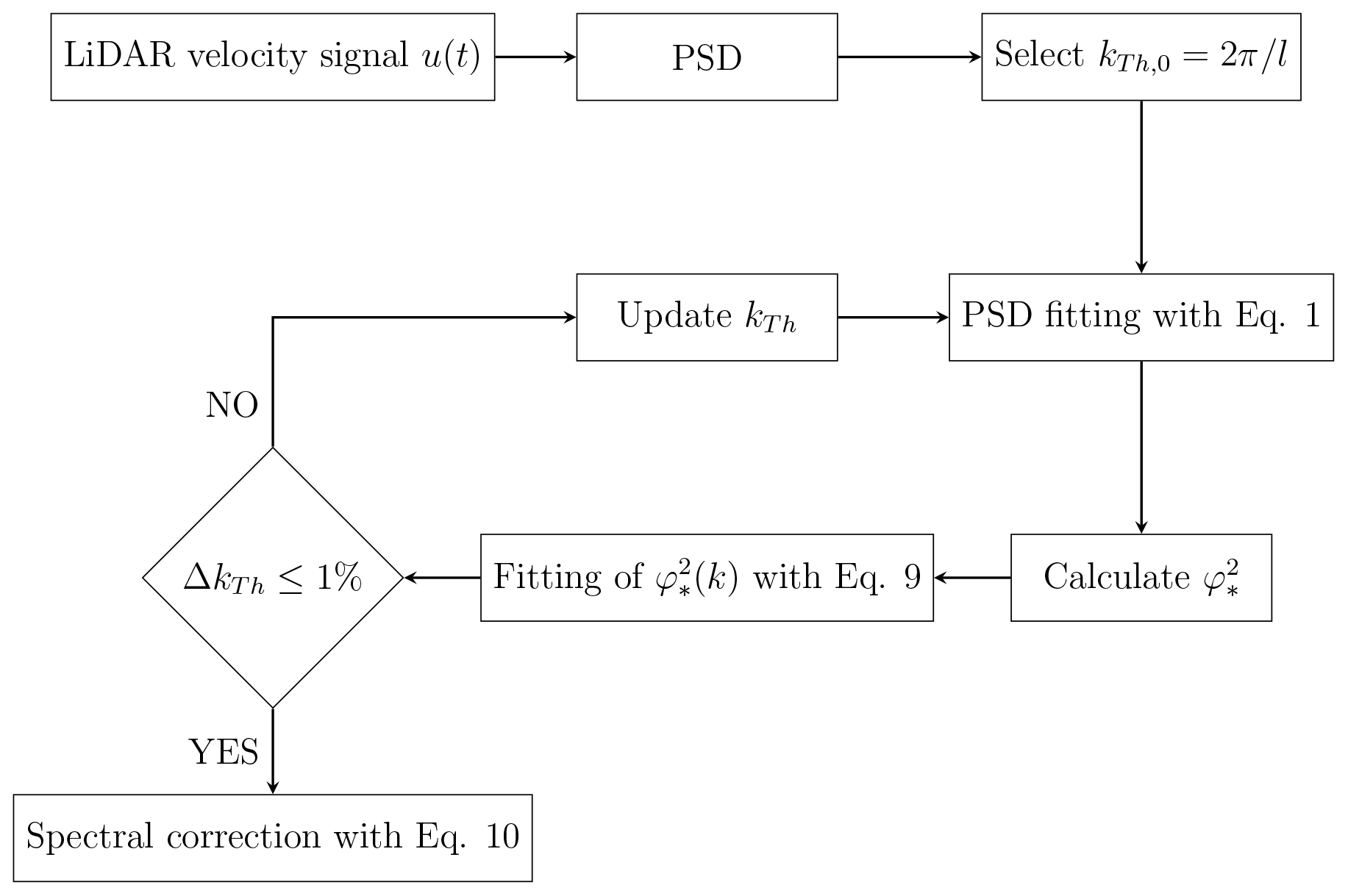
Figure 1 Flowchart for the iterative correction procedure of the lidar velocity measurements.

First, the premultiplied spectrum of the radial velocity projected in the horizontal mean wind direction is fitted with the spectral model of Eq. (1) only for wavenumbers smaller than $k_{\mathrm{Th},\mathrm{0}}=\mathrm{2}\mathit{\pi }/l$. Indeed, we expect to observe significant spatial-averaging effects for turbulent length scales smaller than the probe length, l. For wavenumbers higher than the selected cutoff value, the ratio between the fitted Kaimal spectrum and the PSD of the lidar velocity, ${\mathit{\phi }}_{*}^{\mathrm{2}}$, is calculated to quantify the effect of the energy damping due to the lidar measuring process. Subsequently, the lidar-to-Kaimal ratio, ${\mathit{\phi }}_{*}^{\mathrm{2}}$, is fitted with Eq. (9) through a least-square algorithm to estimate the filter order, α, and provide an updated value for the cutoff wavenumber, k_Th. This process is iterated until convergence on the parameter k_Th is achieved (for this work, the convergence condition imposed is a variation of k_Th smaller than 1 % of the previous value). If, during the iterative process, k_Th achieves a value equal to or smaller than that corresponding to the spectral peak, k_p, then the procedure is arrested and a warning is dispatched indicating that the correction procedure was not successful. This warning condition never occurred for all the data analyzed in this work. Furthermore, it should be considered that when k_Th achieves values close to k_p, the part of the velocity spectrum, S_u, used for the fitting procedure with Eq. (1) can be so limited to jeopardize the accuracy of the fitting procedure. Once convergence in k_Th is achieved, the corrected velocity spectrum, ${\stackrel{\mathrm{̃}}{S}}_L\left(k\right)$, is calculated as

$$\begin{array}{}\text{(10)}& {\stackrel{\mathrm{̃}}{S}}_L\left(k\right)={\displaystyle \frac{S_L\left(k\right)}{{\stackrel{\mathrm{̃}}{\mathit{\phi }}}^{\mathrm{2}}\left(k\right)}}.\end{array}$$

It is noteworthy that in contrast to existing models using predefined functions to correct the energy damping of the velocity fluctuations (see, e.g., Eqs. 5 and 6) (Sjöholm et al., 2009; Brugger et al., 2016; Cheynet et al., 2017), which require information about the lidar probe length and the energy distribution over a pulse, the proposed procedure calculates the characteristics of the damping on the lidar velocity signals directly from the experimental data, which leads, as will be shown in the following, to enhanced accuracy in the correction of the lidar velocity spectra. On the other hand, the proposed procedure leverages the surface-layer similarity for the Kaimal spectral model for the streamwise velocity and, thus, it can only be applied for wind lidar measurements collected within the ASL.

3 Experimental Setup and selected lidar datasets

The present study is based on wind lidar measurements collected from three different experimental campaigns. The first dataset was acquired during the period from 9–24 June 2018 at the Surface Layer Turbulence and Environmental Science Test (SLTEST), which is part of the U.S. Dugway Proving Ground facility in Utah (GPS location: 40^∘08^′07^′′ N, 113^∘27^′04^′′ W, UTC offset −6 h). Characterized by an elevation variability of 1 m every 13 km (Kunkel and Marusic, 2006; Metzger and Klewicki, 2001), this facility is located in the southwest of the Great Salt Lake and extends for 240 and 48 km along north–south and east–west directions, respectively. An aerial view of the SLTEST facility is reported in Fig. 2a. During the experiment, the prevailing wind direction was from the north-northeast.

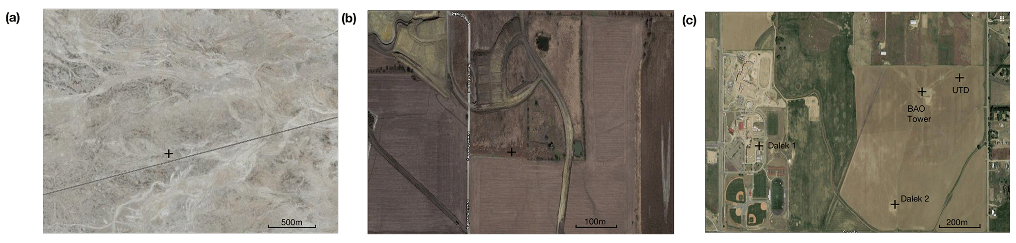
Figure 2 Aerial views of the test sites: (a) SLTEST facility; (b) Celina site; and (c) XPIA campaign at the Boulder Atmospheric Observatory. Source © Google Earth. Black crosses represent the instrument locations. In (c), each lidar is labeled with its respective name.

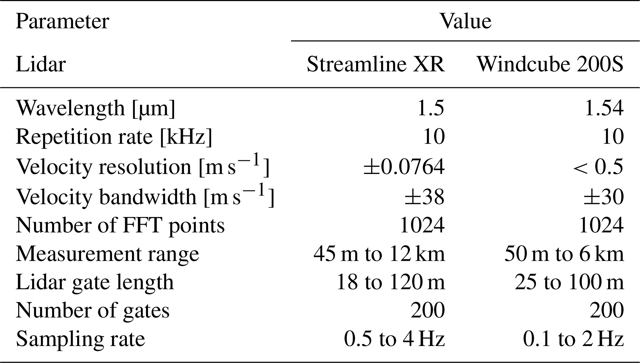
The second field campaign was carried out at a test site in Celina, TX (GPS location: 33^∘17^′35.3^′′ N, 96^∘49^′17.5^′′ W, UTC offset −5 h), which is a relatively flat terrain with a certain variability in land cover (Fig. 2b). For these two field campaigns, wind velocity measurements were performed with a Streamline XR scanning Doppler pulsed wind lidar manufactured by Halo Photonics, whose technical details are reported in Table 1. Lidar fixed scans were performed with an elevation angle between 1.98 and 10^∘, while the azimuth angle was set equal to the mean wind direction. The latter was monitored through vertical azimuth display (VAD) scans with an elevation of 25^∘ and a sampling period of about 90 s, or through Doppler beam swinging (DBS) scans. DBS or VAD scans were executed hourly to monitor variations in the mean wind direction, while the azimuth angle for the fixed scans was updated automatically at the end of each DBS or VAD scan through the feedback scan mode embedded in the lidar software and using the wind direction measured at the height of 53 m. To investigate possible variations of the averaging process related to the accumulation time, the sampling frequency of the fixed scans was varied between 0.5 and 3.3 Hz, while the range gate was always set equal to 18 m.

Table 1 Technical specifications of the pulsed scanning Doppler wind lidars used for this work, namely a Streamline XR by Halo Photonics and a Windcube 200S by Leosphere.

The third campaign considered in this study is the XPIA, performed during the period from 2 March–31 May 2015 at the Boulder Atmospheric Observatory (BAO) research facility in Erie, Colorado. For the XPIA campaign, 12 Campbell CSAT3 3D sonic anemometers were mounted on the BAO meteorological tower at heights of 50, 100, 150, 200, 250, and 300 m above the ground. Each height was monitored with two sonic anemometers pointing towards the northwest and southeast, respectively. Three velocity components and the temperature were recorded with a sampling rate of 20 Hz. For a complete description of the scanning strategies and the instruments utilized during the XPIA experiment see Lundquist et al. (2017). Figure 2c shows the locations of the lidars used.

In the present study, from the XPIA experiment we focus on tests performed during the period from 21–24 March 2015 with a Windcube 200S scanning Doppler pulsed wind lidar manufactured by Leosphere. Technical specifications of the Windcube 200S wind lidar are reported in Table 1. The lidar performed measurements by staring towards one of the sonic anemometers for a period of 14.5 min. A sequential scan at four different heights was done for every hour during each day; details of these tests are available in Debnath (2018). Simultaneous measurements performed with a scanning Doppler wind lidar and sonic anemometers are analyzed to assess the proposed spectral correction procedure of lidar measurements.

For the Celina and SLTEST field campaigns, the regime of the atmospheric stability was monitored through sonic anemometers mounted at a height of 3 m in the proximity of the lidar location. The sampling frequency of the sonic anemometer data was 20 Hz, while atmospheric stability was characterized through the Obukhov length calculated as follows (Monin and Obukhov, 1954):

$$\begin{array}{}\text{(11)}& L=-{\displaystyle \frac{{\mathit{\theta }}_{\mathrm{v}}{u}_{\mathit{\tau },\mathrm{S}}^{\mathrm{3}}}{\mathit{\kappa }g\stackrel{\mathrm{‾}}{w^{\prime }{\mathit{\theta }}_{\mathrm{v}}^{\prime }}}},\end{array}$$

where κ=0.41 is the von Kármán constant, g is the gravitational acceleration, $\stackrel{\mathrm{‾}}{w^{\prime }{\mathit{\theta }}_v^{\prime }}$ is the sensible heat flux, θ_v is the average virtual potential temperature (in Kelvin), and u_τ,S is the friction velocity calculated from sonic anemometer data as (Stull, 1988):

$$\begin{array}{}\text{(12)}& u_{\mathit{\tau },\mathrm{S}}={\left({\stackrel{\mathrm{‾}}{u^{\prime }{w}^{\prime }}}^{\mathrm{2}}+{\stackrel{\mathrm{‾}}{v^{\prime }{w}^{\prime }}}^{\mathrm{2}}\right)}^{\mathrm{1}/\mathrm{4}}.\end{array}$$

To avoid effects of thermal stratification and buoyancy on our analysis, only datasets acquired under near-neutral conditions are considered, which are selected by imposing the threshold $|z/L|\le \mathrm{0.05}$ (Kunkel and Marusic, 2006; Liu et al., 2017).

The lidar velocity signals undergo a quality control process to ensure statistical significance and accuracy of the measurements. Only datasets with a variability of the 10 min averaged wind direction within the range ±20^∘ have been considered to avoid significant offset between the lidar azimuth angle and the instantaneous wind direction (Hutchins et al., 2012).

The quality of the lidar signals is then checked based on the intensity of the back-scattered signal. For the Windcube 200S lidar, the samples with a carrier-to-noise ratio (CNR) higher than −25 dB are selected, while for the Streamline XR lidar data are analyzed only if the intensity of the back-scattered signal is higher than 1.01.

The statistical steadiness of the lidar signals is estimated for both first- and second-order statistics. For the mean velocity, the absolute percentage error is calculated as follows:

$$\begin{array}{}\text{(13)}& {\mathit{\epsilon }}_M={\displaystyle \frac{\frac{\mathrm{1}}{N}{\sum }_{j=\mathrm{1}}^N|U_j-U_{\mathrm{tot}}|}{U_{\mathrm{tot}}}},\end{array}$$

where U_j is the mean wind velocity as a function of height, z, calculated for the jth subperiod of the velocity signal with a duration of 5 min, U_tot is the mean wind velocity as a function of height for the entire velocity signal, while N is the total number of subperiods generated without overlapping. A similar parameter ε_σ is calculated for the second-order statistics (Foken and Wichura, 1996):

$$\begin{array}{}\text{(14)}& {\mathit{\epsilon }}_{\mathit{\sigma }}={\displaystyle \frac{\frac{\mathrm{1}}{N}{\sum }_{j=\mathrm{1}}^N\left({\mathrm{CV}}_j-{\mathrm{CV}}_{\mathrm{tot}}\right)}{{\mathrm{CV}}_{\mathrm{tot}}}},\end{array}$$

where CV_j is the variance of the jth subperiod with a duration of 5 min, while CV_tot is the variance of the signal over the entire period. For Celina and SLTEST campaigns, the parameters ε_M and ε_σ were calculated for 1 h periods, while for the XPIA deployment the whole 14.5 min record was analyzed. For quality control purposes, signals with ε_M≥15 % or ε_σ≥40 % are usually rejected (Foken and Wichura, 1996; Foken et al., 2004). The parameters ε_M and ε_σ are calculated for each range gate and their maximum values for the selected datasets are reported in Table 2.

Subsequently, a gradient-based procedure is used to remove outliers from the lidar radial velocity signals. Specifically, the partial derivative in time of the radial velocity is calculated through a second-order central finite-difference scheme, and velocity samples with absolute partial derivative larger than 15 times the respective median value calculated over the entire signal are marked as outliers and replaced through the inpaint-nans function available in Matlab (D'Errico, 2004). The used threshold value is selected based on a sensitivity analysis. Based on the above-mentioned quality-control procedure, five datasets were selected, whose details are reported in Table 2.

Table 2 Description of the selected datasets: Φ is the lidar elevation angle, f_S is the sampling frequency, l is the probe length, ϵ_M is the absolute percentage error on the mean velocity, ϵ_σ is the percentage error on the velocity variance, u_τ is the friction velocity, and z₀ is the aerodynamic roughness length. The last column reports the symbol used for each dataset.

The radial velocity, V_r, measured by a Doppler wind lidar, as explained in Sect. 2, is expressed as

$$\begin{array}{}\text{(15)}& V_{\mathrm{r}}=V_{\mathrm{h}}\cos (\mathit{\theta }-{\mathit{\theta }}_{\mathrm{w}})\cos \mathrm{\Phi }+W\sin \mathrm{\Phi },\end{array}$$

where θ and Φ are the lidar azimuth and elevation angles, respectively, θ_w is the wind direction, and V_h and W are the horizontal and vertical wind velocities, respectively. As previously mentioned, for the SLTEST and Celina field campaigns, lidar measurements were carried out with the azimuth angle equal to the mean wind direction and very low elevation angles (Table 2). Therefore, we can calculate an approximation of the horizontal wind speed as

$$\begin{array}{}\text{(16)}& U_{\mathrm{eq}}=V_{\mathrm{r}}/\cos \mathrm{\Phi },\end{array}$$

which is referred to as horizontal equivalent velocity. In the following, U_eq is considered to calculate the streamwise velocity spectrum. Furthermore, the variance of the radial velocity is the first-order approximation of the streamwise-velocity variance given the above-mentioned setup constraints (Eberhard et al., 1989; Sathe and Mann, 2013).

4 Assessment of the lidar spectral correction against sonic anemometry

In this section, the procedure proposed in Sect. 2 to correct the energy damping in the lidar velocity measurements due to the energy pulse distribution over the probe volume is assessed against sonic anemometry by leveraging the XPIA dataset, whose characteristics are summarized in Table 2. Lidar fixed scans were performed with an elevation angle of 5^∘ to have one range gate in the proximity of a sonic anemometer installed on the BAO tower at a height of 100 m. The lidar probe length used for that experiment was equal to 50 m, while the sampling rate was set equal to 2 Hz.

Based on the instantaneous wind direction measured by the sonic anemometer and neglecting the vertical velocity due to the very low elevation angle of the lidar laser beam, the horizontal equivalent velocity, U_eq, is calculated from the lidar radial velocity through Eq. (15) and it is reported in Fig. 3 with a blue line. The lidar equivalent velocity, U_eq, is then high-pass filtered to remove low-frequency non-turbulent velocity fluctuations, using the following spectral transfer function:

$$\begin{array}{}\text{(17)}& G(k;\mathit{\beta },k_{\mathrm{co}})={\displaystyle \frac{\mathrm{1}+\tanh \left[\mathit{\beta }\cdot \log \left(\frac{k}{k_{\mathrm{co}}}\right)\right]}{\mathrm{2}}},\end{array}$$

where k_co is the cutoff wavenumber, which should be smaller than k_p to avoid effects on the spectral peak. The parameter β is set equal to 100 to generate a sufficiently sharp filter across the cutoff wavenumber, k_co (Hu et al., 2020). The PSD of the velocity signal high-pass filtered with a cutoff wavenumber $k_{\mathrm{co}}=\mathrm{1.26}\times {\mathrm{10}}^{-\mathrm{3}}$ m⁻¹ is reported in Fig. 4a with a gray line.

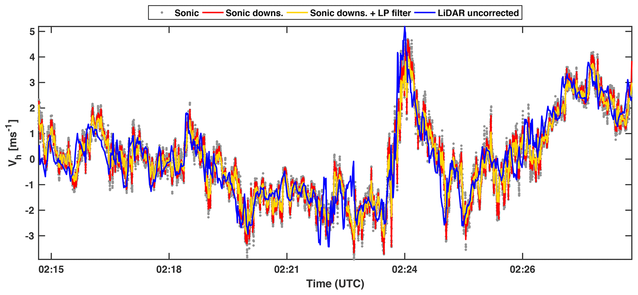
Figure 3 Subset of the horizontal velocity measured with a lidar and sonic anemometer from the XPIA dataset. The gray dots represent the original 20 Hz sampled sonic-anemometer data, the red line is the sonic anemometer signal downsampled at 2 Hz, the yellow line is the sonic anemometer signal after the convolution of Eq. (9), and the blue line is the lidar signal before the spectral correction.

Figure 4 Correction of the lidar velocity spectrum from the XPIA dataset: (a) velocity spectra of the raw lidar data (gray), lidar data after application of the denoising procedure (To et al., 2009) (light blue), lidar data after smoothing procedure (dark blue), Kaimal spectrum (black), and $-\mathrm{5}/\mathrm{3}$ slope (black dashed); (b) $|{\mathit{\phi }}_{*}{|}^{\mathrm{2}}$ (blue), $|{\mathit{\phi }}_{*}{|}^{\mathrm{2}}$ fitted with Eq. (9) (black); predictions from Eq. (5) (bright green) and Eq. (6) (dark green) are reported as well.

In case significant noise in the velocity spectra is observed in the proximity of the Nyquist wavenumber (see, e.g., Debnath (2018)), as for this velocity signal, a denoising procedure is then applied to remove possible noise effects on the velocity signals. Following the wavelet-transform-based procedure proposed by To et al. (2009), the velocity signal is decomposed in a 10-level orthogonal wavelet basis. For each level, a soft-threshold selection is applied to the wavelet coefficients to remove those related to noise. The estimated noise-free wavelet coefficients, d_jk, are calculated as

$$\begin{array}{}\text{(18)}& {\mathrm{d}}_{jk}=\left\{\begin{array}{ll}\mathrm{sgn}\left(w_{jk}\right)\left(\right|w_{jk}|-T_j)& \mathrm{if}\left|w_{jk}\right|>T_j\\ \mathrm{0}& \mathrm{otherwise}\end{array},\right.\end{array}$$

where $j=\mathrm{1},\mathrm{\dots },\mathrm{10}$ is the number of levels in the wavelet basis; $k=\mathrm{1},\mathrm{\dots },{\mathrm{2}}^j$, and w_jk are the coefficients of the discrete wavelet transform of the original signal. T_j represents a noise-based threshold for the jth level that for this work is set to (To et al., 2009)

$$\begin{array}{}\text{(19)}& T_j={\displaystyle \frac{\mathrm{med}\left(\right|w_{jk}\left|\right)}{\mathrm{0.67}}}\cdot \sqrt{\mathrm{2}\log {\mathrm{2}}^j},\end{array}$$

where med(⋅) stands for the median value. Finally, the denoised signal is reconstructed in time through the modified wavelet coefficients d_jk. The spectrum of the denoised lidar velocity signal is reported in Fig. 4a with a light-blue line.

For modeling purposes, the velocity spectra are then smoothed in the wavenumber domain following the Savitzky–Golay filter (Savitzky and Golay, 1964) by using a second-order polynomial function and windows with the width equal to int[10(160k)^0.5], where k is in m⁻¹ and int is rounded to the closest integer number (Balasubramaniam, 2005). The result is an increased level of smoothness moving towards the Nyquist wavenumber. The lidar velocity spectrum resulting from the denoising and smoothing procedures is reported in Fig. 4a with a blue line. The PSD of the lidar velocity is then fitted through the spectral model (Eq. 1) producing the following fitting parameters: A=23.3, B=24.7. The resulting Kaimal spectrum is plotted in Fig. 4a with a black line.

A deviation of the lidar velocity spectrum from the $-\mathrm{5}/\mathrm{3}$ scaling of the inertial subrange is observed due to the lidar measuring process over the probe volume. The ratio between the fitted Kaimal spectrum and the lidar velocity spectrum, $|{\mathit{\phi }}_{*}{|}^{\mathrm{2}}$ in Fig. 4b, is then fitted with Eq. 9 to estimate the low-pass filter of order α and cutoff wavenumber, k_Th. For this lidar velocity signal, α is equal to 0.774 and $k_{\mathrm{Th}}l/\left(\mathrm{2}\mathit{\pi }\right)\approx \mathrm{0.8}$, with an R² value of 0.702, which confirms the proposed model is a good approximation for the damping of the velocity fluctuations over the lidar probe volume. In Fig. 4b, the weighting functions of Eqs. (5) and (6) are also reported for a probe length l=50 m.

To assess the accuracy of the estimated low-pass filter in representing the lidar averaging process over a probe volume, first we apply the estimated low-pass filter to the simultaneous and colocated sonic anemometer velocity signal. The horizontal velocity retrieved from the sonic anemometer is first down-sampled with the sampling frequency of the lidar measurements, namely 2 Hz, using the Matlab function “decimate” with a finite-impulse response (FIR) low-pass filter with order equal to 10 (Weinstein, 1979). The resulting down-sampled velocity signal is reported with a red line in Fig. 3 and the respective PSD in Fig. 5a. Subsequently, the down-sampled sonic-anemometer signal is low-pass filtered with the filter of Eq. (9) modeled only using the lidar data (yellow line in Figs. 3 and 5a). The comparison in Fig. 3 of the sonic anemometer signal down-sampled and low-pass filtered with the lidar raw signal already highlights a very good agreement, which suggests that the energy damping carried out by the lidar pulse over the probe volume is well represented through the proposed low-pass filter. This feature is further corroborated by the respective spectra reported in Fig. 5a. Specifically, the spectrum of the LOS velocity has the same slope in the inertial subrange of the sonic-anemometer signal down-sampled and low-pass filtered, while some differences are observed for lower frequencies, which are most probably due to the different size of the measurement volume of the two instruments, namely 50 m for the lidar and 0.3 m for the sonic anemometer.

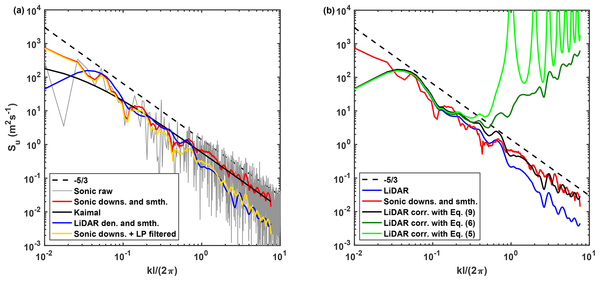
Figure 5 Comparison of lidar velocity data against sonic anemometry data for the XPIA dataset: (a) raw sonic anemometer data (gray), down-sampled and smoothed sonic anemometer (red), Kaimal model (black) tuned on the lidar velocity spectrum (blue), and sonic anemometer signal down-sampled and low-pass filtered (yellow); (b) lidar velocity spectrum (blue), down-sampled and smoothed sonic anemometer spectrum (red), and lidar spectrum corrected with Eqs. (9), (5), and (6) (black, bright green, and dark green lines, respectively).

The comparison between lidar and sonic anemometer data is now presented through a linear regression analysis, which is reported in Fig. 6. The lidar horizontal equivalent velocity, U_eq, is analyzed against the horizontal wind speed measured by the sonic anemometer before (Fig. 6a) and after (Fig. 6b) the low-pass filtering. All the linear regression parameters improve for the low-pass filtered sonic anemometer data: the slope increases from 0.878 to 0.962, the R-square value increases from 0.88 to 0.904, and the correlation coefficient, ρ, increases from 0.88 to 0.904.

Figure 6 Linear regression between lidar horizontal equivalent velocity, U_eq, and sonic anemometer horizontal velocity from the XPIA dataset: (a) raw data from the sonic anemometer and (b) sonic anemometer data down-sampled and low-pass filtered.

We now aim to correct the lidar velocity signal from the energy damping due to the laser pulse distribution over the probe volume. First, the lidar velocity spectrum is corrected by using the existing models of Eqs. (5) and (6) with l=50 m, i.e., the used lidar probe length. As shown in Figs. 4b and 5b, these correction methods largely over-estimate the turbulent energy for wavenumbers larger than k_Th or, in other words, the characteristic length scale should be smaller than the lidar probe length to provide reasonable spectral corrections. A possible explanation for the poor performance of these deconvolution models could be the presence of residual noise in the data, which is not accounted for in the models of Eqs. (5) and (6). Other factors, like the different probe length used for the XPIA campaign (l=50 m) in contrast to l=30 m used in the original study of this deconvolution model (Mann et al., 2009), are thought to have marginal effects on the estimation of the energy spectrum at higher frequencies.

According to the correction technique proposed in this paper, the lidar velocity spectrum can now be corrected for the averaging process by reversing the effect of the estimated low-pass filter through Eq. (10). The corrected velocity spectrum is reported in Fig. 5b with a black line. The velocity spectrum of the corrected lidar velocity signal clearly shows that the expected slope of $-\mathrm{5}/\mathrm{3}$ in the inertial subrange is recovered, while the spectral energy for lower wavenumbers is practically unchanged.

5 Variability of the low-pass filter parameters

For the SLTEST and Celina field campaigns, lidar velocity measurements were collected for periods between 2 and 3 h (see Table 2). The procedure used to obtain the streamwise velocity spectra is the following: for each lidar velocity signal, the high-pass filter of Eq. (17) is applied with a cutoff wavenumber k_co=0.001 m⁻¹ to remove low-frequency velocity fluctuations connected with atmospheric mesoscales. The PSD of each velocity signal is then calculated with the pwelch function implemented in Matlab (Welch, 1967) without window overlapping and window width corresponding to k_co. Subsequently, smoothing of the velocity spectra is carried out through the Savitzky–Golay filter, as detailed in the previous section (Savitzky and Golay, 1964; Balasubramaniam, 2005).

The mean values and variance of the lidar equivalent velocity are plotted in Fig. 7a and b, respectively. For the mean velocity field in Fig. 7a, while a logarithmic region is generally observed at the lower heights, a noticeable difference in terms of terrain roughness between the SLTEST and Celina sites results in different vertical intercepts and respective aerodynamic roughness length. The latter is estimated to be equal to 0.021 mm for SLTEST and, on average, 37 mm for the Celina site.

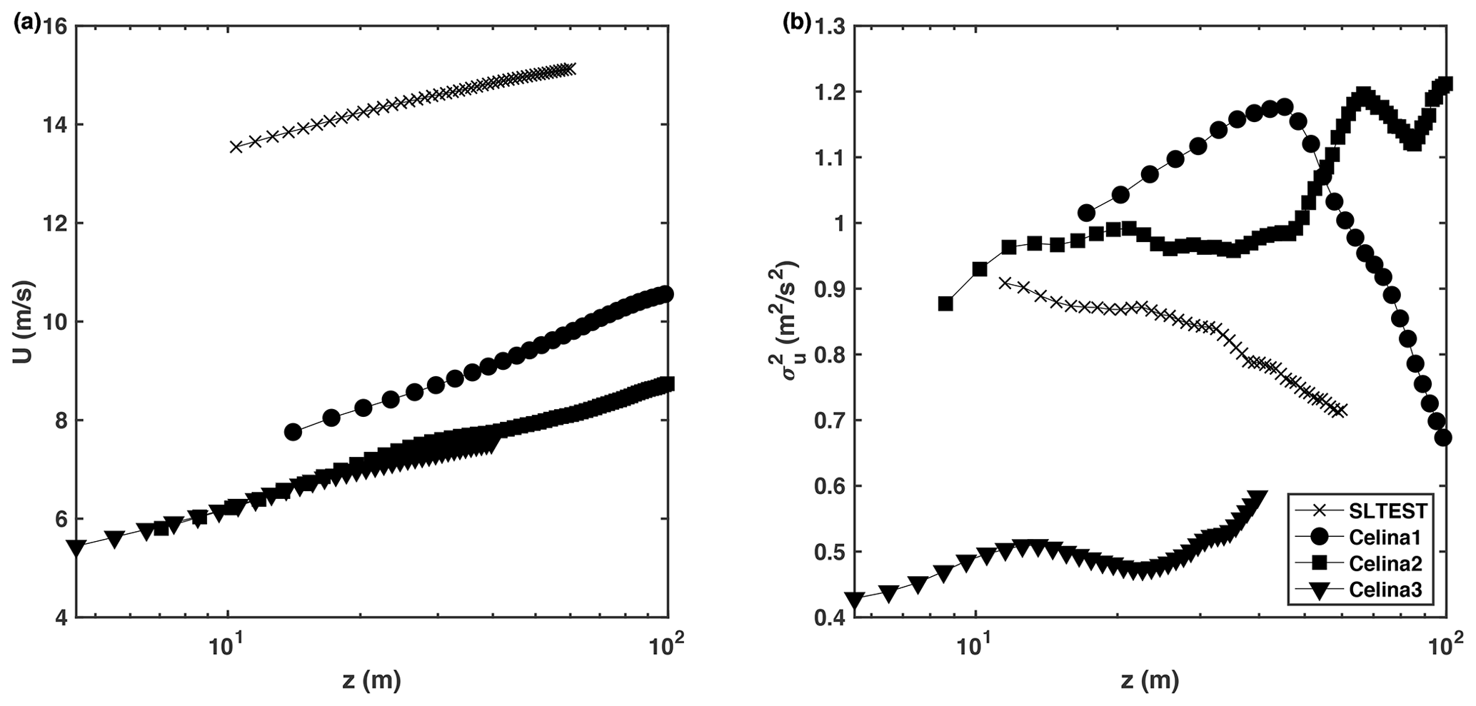
Figure 7 First- and second-order statistics of the equivalent velocity, U_eq, as a function of height for the various datasets: (a) mean value and (b) variance.

The vertical profiles of streamwise velocity variance are reported in Fig. 7b as a function of height. For the datasets collected at the Celina site, a general increase of the velocity variance is observed with increasing height. Specifically, for the dataset Celina1, after achieving a maximum value at height z≥40 m, a quasi-logarithmic reduction of the velocity variance is observed with increasing height, which is in agreement with previous laboratory and numerical studies of canonical boundary layer flows (Kunkel and Marusic, 2006; Meneveau and Marusic, 2013). A logarithmic reduction of the velocity variance with increasing height is also observed for the SLTEST dataset throughout the entire height range.

For the SLTEST dataset, the PSD of the lidar velocity signals acquired at the different gates from 10 up to 60 m with a vertical spacing of 1 m are plotted in Fig. 8. A departure from the expected $-\mathrm{5}/\mathrm{3}$ slope in the inertial subrange is observed for wavenumbers larger than 0.07 m⁻¹. The Kaimal spectra, which are obtained by fitting the measured lidar velocity spectra only for wavenumbers lower than the respective k_Th for each height, are reported in Fig. 9a for the lowest and highest range gates. The ratio between the lidar and Kaimal spectra, $|{\mathit{\phi }}_{*}{|}^{\mathrm{2}}$, is then calculated and fitted through Eq. (9) to estimate the order and cutoff wavenumber of the respective low-pass filter (Fig. 9b). For the lowest gate at a height of 10 m, the fitting procedure estimated α=5.08 and k_Th=0.065 m⁻¹, while for the highest range gate at a height of 60 m, α=4.16 and k_Th=0.066 m⁻¹.

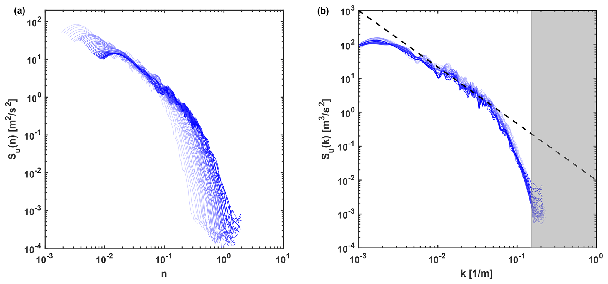
Figure 8 Velocity spectra for the SLTEST dataset at different heights: (a) spectra as a function of the reduced frequency, n, and (b) spectra as a function of the wavenumber, k. Line color is darker with increasing height. The black dashed line represents the $-\mathrm{5}/\mathrm{3}$ slope. In (b), the shaded area covers the noisy part of the velocity spectra.

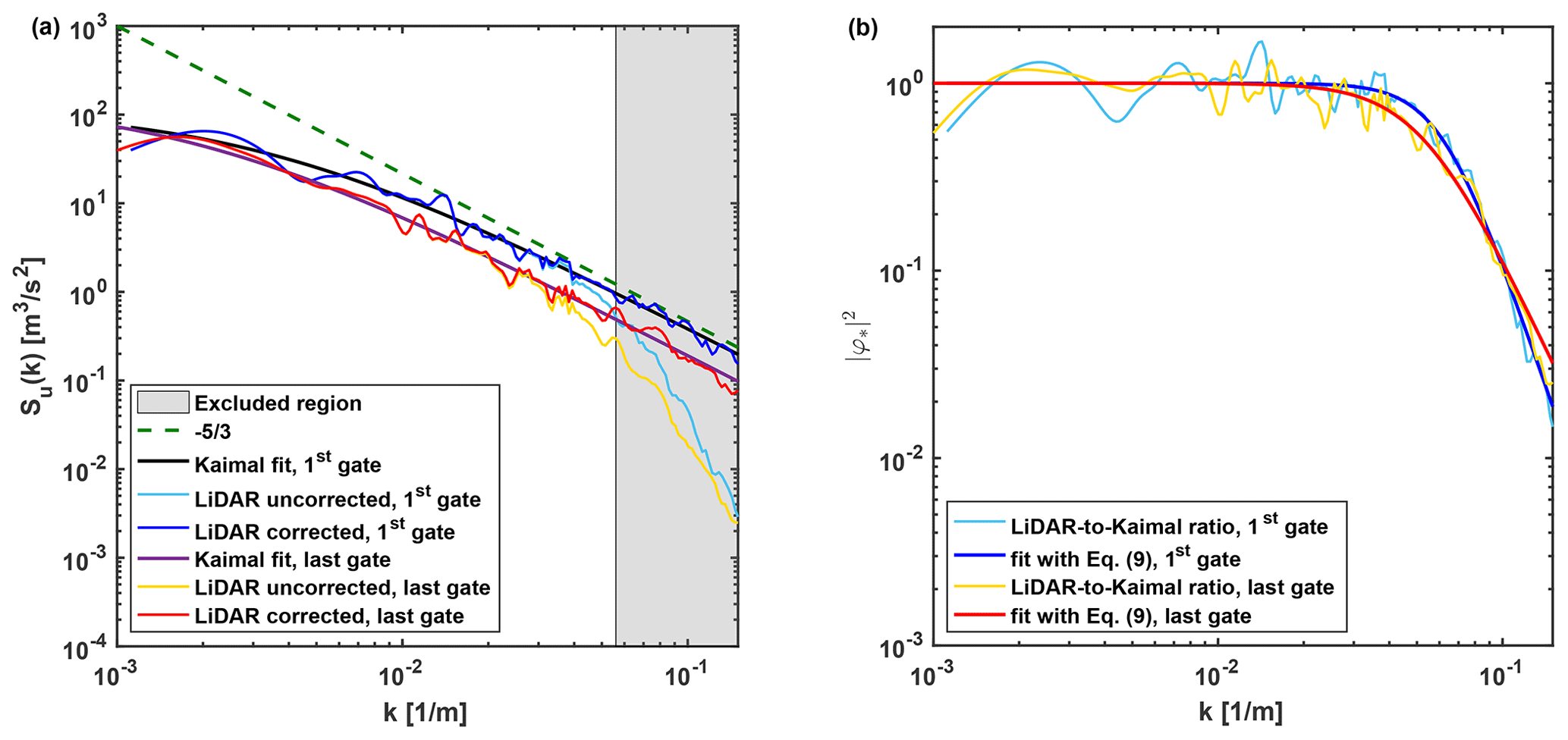
Figure 9 Lidar velocity signals from the SLTEST dataset acquired at z=10 m (first gate, dark and light blue lines) and z=60 m (last gate, red and yellow lines): (a) correction of the lidar spectra and (b) ratio between lidar and Kaimal spectra, ${\mathit{\phi }}_{*}^{\mathrm{2}}$, and low-pass filter fitted with Eq. (9).

Since the correction procedure is based on two consecutive best-fit operations, the robustness of the model is assessed for each lidar gate through the R-square value of the respective fitting procedure. All the datasets generally show a very good agreement between experimental data and the spectral model, i.e., $\mathrm{0.82}\le R^{\mathrm{2}}\le \mathrm{0.98}$, with the SLTEST dataset showing the highest level of agreement (R²≥0.96). Accuracy in modeling the actual energy damping due to the lidar measuring process through the low-pass filter of Eq. (9) is quantified through the R-square value of the fitting procedure of the experimental energy damping, ${\mathit{\phi }}_{*}^{\mathrm{2}}$, with the analytical model of Eq. (9). The resulting R-square values are always larger than 88 %, corroborating the good approximation for the proposed model.

The proposed spectral correction of the lidar measurements is now applied to all the datasets collected at the Celina and SLTEST sites (see Table 2). As explained in Sect. 2, the first step of the proposed procedure consists of fitting each velocity spectrum with the spectral model of Eq. (1). In the right column of Fig. 10, the results of this operation are reported for all the datasets of the SLTEST and Celina field campaigns. The spectral model (depicted with a red line) has been fitted on the uncorrected lidar spectrum (blue lines) using a cutoff wavenumber, k_Th, estimated for each velocity signal using the iterative procedure illustrated in Fig. 1. In the figures, line colors become darker with increasing height. For the sake of clarity, the fitted Kaimal spectrum is only shown for the highest lidar range gate.

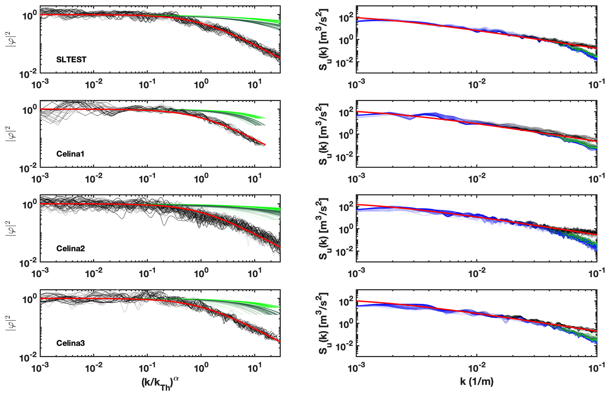
Figure 10 Correction of the lidar spectra. Left column: the black lines are ${\mathit{\phi }}_{*}^{\mathrm{2}}$ and the red line is the fitted low-pass filters of Eq. (9) for the highest range gate. Dark and light green lines represent the transfer function predicted by Eqs. (5) and (6). Right column: the blue lines are raw lidar spectra, the dark and light green lines are lidar spectra corrected with Eqs. (5) and (6), respectively, the red line is the fitted Kaimal spectrum for the highest range gate, and the black lines are the lidar spectra corrected with the proposed procedure of Fig. 1. Line colors become darker with increasing height.

The second step of the correction procedure consists of approximating the lidar-to-Kaimal spectral ratio with the low-pass filter of Eq. (9). Firstly, the energy ratio is quantified for each lidar range gate, as reported in the left column of Fig. 10. We can observe that the ratio always settles about the unit at the lowest range of the spectral domain, while it monotonically reduces from the cutoff wavenumber towards the Nyquist wavenumber, which is an effect of the lidar measuring process. By plotting $|{\mathit{\phi }}_{*}{|}^{\mathrm{2}}$ as a function of $(k/k_{\mathrm{Th}}{)}^{\mathit{\alpha }}$, all the estimated transfer functions practically collapse on the same curve for measurements collected at different heights. The latter is then compared with the sanalogues of Eqs. (5) and (6).

As the last step, to retrieve the corrected lidar velocity spectra, the original spectrum is divided by the modeled correction function, $|\stackrel{\mathrm{̃}}{\mathit{\phi }}{|}^{\mathrm{2}}$ (Eq. 10). These corrected lidar velocity spectra are reported in the right column of Fig. 10, where we can observe that the $-\mathrm{5}/\mathrm{3}$ slope of the inertial subrange is always recovered. The lidar spectra corrected with the models of Eqs. (5) and (6) are also reported to highlight the improved accuracy achieved through the proposed method. In particular, it is observed that the existing models of Eqs. (5) and (6) always underestimate the spectral energy attenuation; thus, for the actual choices of gate length and sampling rates, a data-driven approach is preferred to correct the lidar smoothing effect.

The corrected variance of the lidar velocity signals is compared with the respective quantity calculated for the raw lidar data in Fig. 11a. As expected, the wall-normal profile of the variance calculated as the integral of the deconvoluted spectrum is considerably larger than the respective value obtained from the convoluted spectrum, indicating that the underestimation related to the spatial averaging is significant. To quantify the effects of the spectral correction on the lidar data, the relative percentage increment of variance is calculated from the smallest frequency up to the noise-free high-frequency content as in Cheynet et al. (2017):

$$\begin{array}{}\text{(20)}& {\mathit{ϵ}}_{\mathit{\%}}={\displaystyle \frac{{\mathit{\sigma }}_{\mathrm{C}}^{\mathrm{2}}-{\mathit{\sigma }}_{\mathrm{U}}^{\mathrm{2}}}{{\mathit{\sigma }}_{\mathrm{C}}^{\mathrm{2}}}}\cdot \mathrm{100},\end{array}$$

where ${\mathit{\sigma }}_{\mathrm{C}}^{\mathrm{2}}$ and ${\mathit{\sigma }}_{\mathrm{U}}^{\mathrm{2}}$ are the corrected and uncorrected, respectively, streamwise velocity variance. The parameter ϵ_% is reported as a function of height in Fig. 11b. The underestimation in the velocity variance through the lidar measurements seems to change with the wall-normal location for the SLTEST dataset and the highest portion of Celina1 (z>30 m); for the remaining datasets, the percentage error does not change with height. To clarify this aspect, in the next section we will investigate the variability of the effects of the lidar spatial averaging for different mean wind speed, standard deviation, and sampling height.

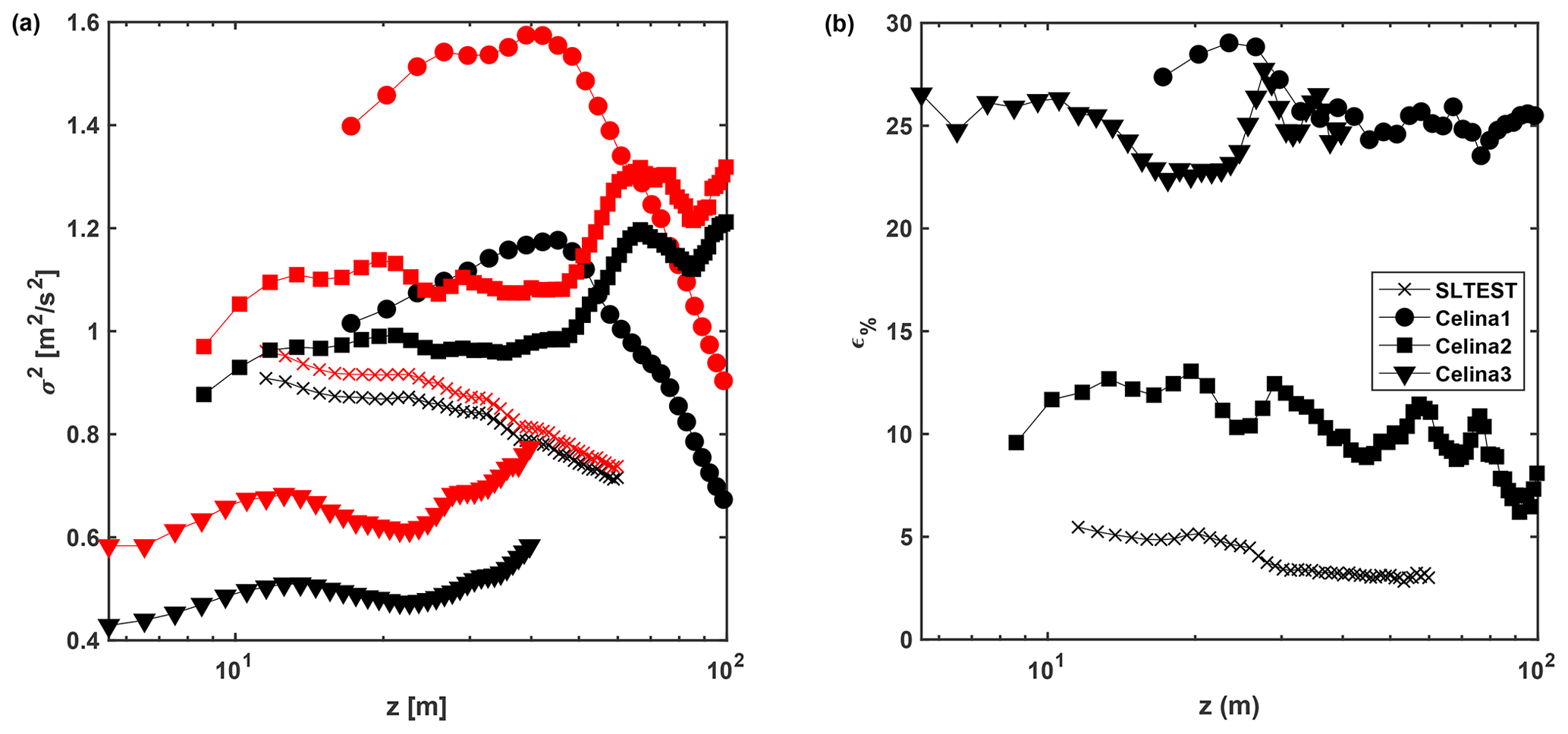
Figure 11 Correction of the second-order statistics: (a) variance before (black) and after (red) the lidar spectral correction and (b) percentage increment of the velocity variance(ϵ_%) achieved with the lidar spectral correction.

For the SLTEST dataset (see Table 2), the correction of the velocity variance obtained with the proposed method (red marker in Fig. 12a) is compared with those obtained from Eq. (5) (dark green symbols), Eq. (6) (light green marker), and the method of Brugger et al. (2016) (blue marker). For the latter, a probe length of 18 m and a full-width half-maximum (FWHM) of the laser pulse for the Streamline XR Doppler lidar equal to 35 m are used (Risan et al., 2018). Consistently with the spectra of Fig. 10, the correction methods of Eqs. (5) and (6) underestimate the effects of spatial averaging of the streamwise velocity variance and they do not allow the complete recovery of the $-\mathrm{5}/\mathrm{3}$ slope of the inertial subrange. The correction based on the structure function proposed by Brugger et al. (2016) leads to a variance distribution larger than what is estimated by the new method based on the Kaimal spectral model, yet with percentage correction in the same order of magnitude (Fig. 12b).

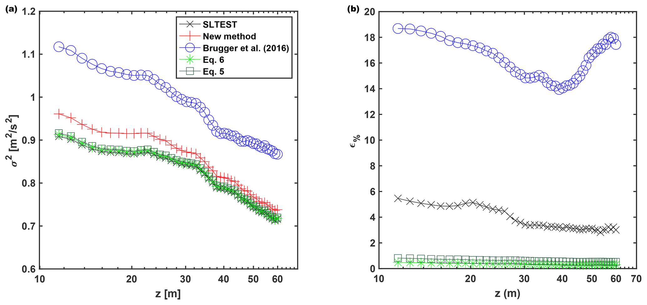
Figure 12 Correction of the streamwise velocity variance with different methods for the SLTEST dataset: (a) streamwise velocity variance and (b) percentage correction of the velocity variance, ϵ_%. The marker colors are black for the raw lidar data, red for the proposed method, light green for Eq. (6), dark green for Eq. (5), and blue for the method proposed by Brugger et al. (2016).

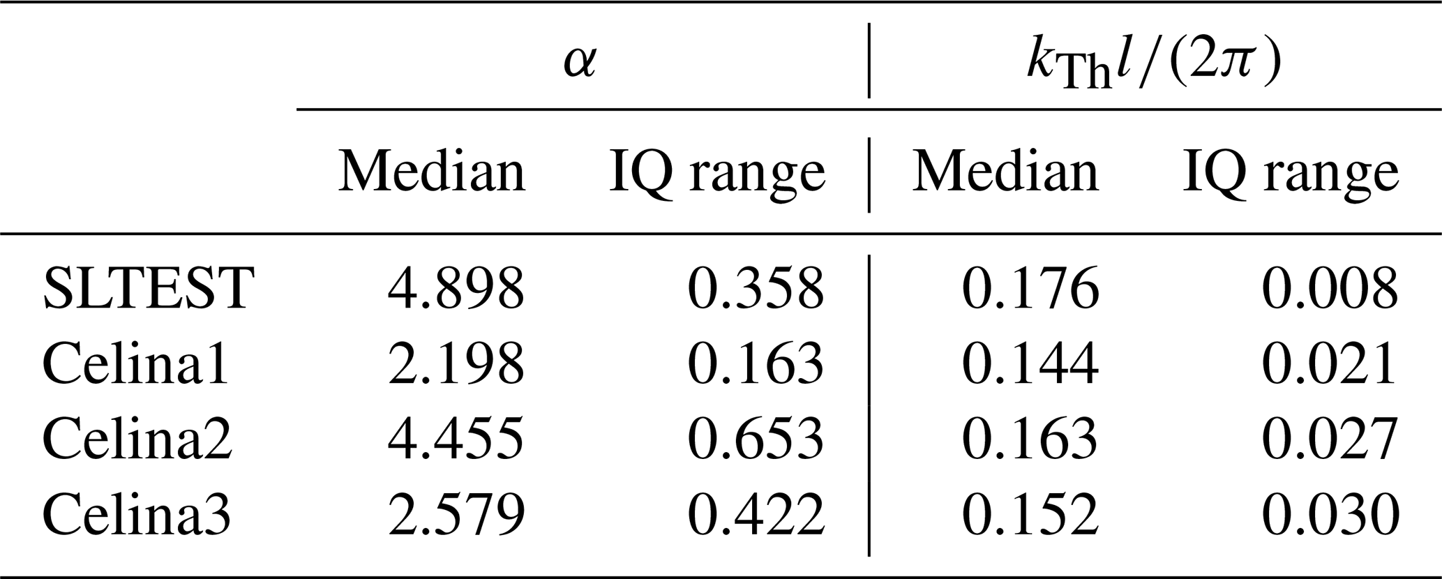
We now focus on the variability of the parameters of the low-pass filter of Eq. (9) among the various datasets. Median and interquartile (IQ) range calculated over the height for the various datasets are reported in Table 3 for both order, α, and cutoff wavenumber, k_Th, of the low-pass filter of Eq. (9). First, the order of the low-pass filter, α, is found to be roughly constant over the height for the Celina1 and Celina3 datasets, while it decreases with height for the SLTEST and Celina2 datasets. Among the various datasets analyzed, the filter order, α, has values from 2.2 up to 4.9, a variation entailing limited effects in the correction of the spatial averaging on the lidar measurements (not shown here for the sake of brevity). The mean IQ range of α among the various datasets is 0.399. The cutoff wavenumber of the low-pass filter, k_Th, is practically constant with height (mean IQ range of 0.022) and has a mean value among the various datasets of: $k_{\mathrm{Th}}l/\left(\mathrm{2}\mathit{\pi }\right)=$0.163.

Table 3 Median and interquartile (IQ) values of the estimated order, α, and cutoff wavenumber, k_Th, of the low-pass filter modeling the lidar spatial averaging for each dataset.

6 Variability in spatial filtering with mean wind speed, turbulence intensity, and sampling height

To investigate the effects of the spatial averaging on wind lidar measurements for different mean wind speed, turbulence intensity, and sampling height of the velocity signals, synthetic turbulent velocity spectra are generated using the spectral model of Eq. (1), while the energy damping connected with the lidar measuring process is estimated through Eq. (9) by using a filter order α=3 and (k_Thl)=0.95, in analogy to the respective experimental values reported in Table 3.

Within the inertial sublayer, namely for heights smaller than about 30 % of the surface layer height (Marusic et al., 2013), the mean streamwise velocity for near-neutral stability conditions can be modeled through the following logarithmic law (Monin and Obukhov, 1954; Stull, 1988):

$$\begin{array}{}\text{(21)}& U={\displaystyle \frac{u_{\mathit{\tau }}}{\mathit{\kappa }}}\log \left({\displaystyle \frac{z}{z_{\mathrm{0}}}}\right),\end{array}$$

where κ=0.41 is the von Kármán constant. Furthermore, we should expect a logarithmic decrease in the velocity variance with increasing wall-normal distance (Townsend, 1976), as follows:

$$\begin{array}{}\text{(22)}& {\displaystyle \frac{{\mathit{\sigma }}^{\mathrm{2}}}{u_{\mathit{\tau }}^{\mathrm{2}}}}=H_{\mathrm{1}}-G_{\mathrm{1}}\log \left({\displaystyle \frac{z}{\mathit{\delta }}}\right),\end{array}$$

where δ is the outer scale of turbulence, namely the boundary layer height, G₁=0.98 is the Townsend–Perry constant (Baars and Marusic, 2020), while H₁ might be dependent on the characteristics of the specific boundary layer flow under investigation. Previous field campaigns performed at the SLTEST site have quantified H₁=2.14 (Marusic et al., 2013).

According to the spectral model of Eq. (1), the velocity variance can be obtained by integrating S_u in the spectral domain, which leads to

$$\begin{array}{}\text{(23)}& {\displaystyle \frac{{\mathit{\sigma }}^{\mathrm{2}}}{u_{\mathit{\tau }}^{\mathrm{2}}}}=\underset{\mathrm{0}}{\overset{\mathrm{\infty }}{\int }}{\displaystyle \frac{A}{{\left(\mathrm{1}+Bn\right)}^{\mathrm{5}/\mathrm{3}}}}\mathrm{d}n={\displaystyle \frac{\mathrm{3}}{\mathrm{2}}}{\displaystyle \frac{A}{B}},\end{array}$$

where A and B vary with the sampling height.

The first analysis is performed by varying the friction velocity, u_τ, within the range between 0.1 and 0.7 m s⁻¹ with a step of 0.05 m s⁻¹, while keeping fixed the sampling height $z/\mathit{\delta }=\mathrm{0.3}$ (B=33 (Kaimal et al., 1972)) and $z_{\mathrm{0}}={\mathrm{10}}^{-\mathrm{4}}$ m. This study aims to investigate variations in lidar spatial averaging for mean wind speed within the range $U\in [\mathrm{3},\mathrm{23}]$ m s⁻¹, while keeping unchanged the turbulence intensity (TI = $\mathit{\sigma }/U=\mathrm{6.29}$ % at $z/\mathit{\delta }=\mathrm{0.3}$). The velocity standard deviation varies linearly with u_τ within the range $\mathit{\sigma }=[\mathrm{0.19},\mathrm{1.35}]$ m s⁻¹ (Eq. 22), and the respective values of the parameter A are calculated from Eq. (23). The probe length, l, is varied from 10 up to 100 m with a step of 10 m.

The parameter ϵ_%, which is defined in Eq. (20), is used to quantify the effects of the lidar spatial averaging on the variance of the wind velocity. In Fig. 13a, it is observed that, as expected, ϵ_% increases with increasing probe length, which indicates that the probe length is the main root cause of spatial averaging. Furthermore, it is noteworthy that for a given value of l, ϵ_% decreases with increasing u_τ and, thus, mean wind speed, U. Indeed, by fixing the probe length, the cutoff wavenumber, k_Th, representing the spatial averaging is, in turn, fixed while the reduction of ϵ_% with increasing U can be explained in the perspective of the Taylor frozen-turbulence hypothesis (Taylor, 1938). In other terms, with increasing U, a turbulent spectrum will shift towards lower wavenumbers (denominator in Eq. 1) and, thus, reduce the percentage of the spectral energy that is filtered for wavenumbers larger than k_Th.

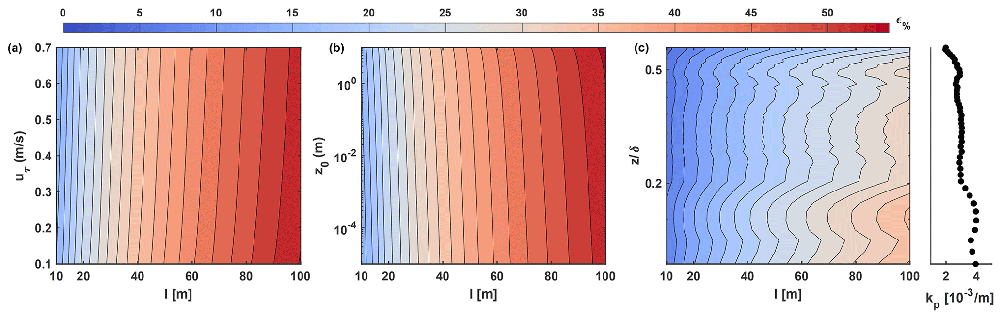
Figure 13 Variation of the percentage variance damping, ϵ_%, connected with the lidar spatial averaging for different probe lengths and wind conditions: (a) variability with the friction velocity, u_τ, (b) variability with the aerodynamic roughness length, z₀, and (c) variability with sampling height, z. The side panel of (c) reports the vertical profile of the parameter k_p estimated for the SLTEST dataset.

The second test case, whose results are reported in Fig. 13b, is performed by varying the aerodynamic roughness length within the range: $z_{\mathrm{0}}=[{\mathrm{10}}^{-\mathrm{5}},\mathrm{10}]$ m, while keeping fixed u_τ= 0.5 m s⁻¹, and sampling height $z/\mathit{\delta }=\mathrm{0.3}$ (B=33). In this case, variations of z₀ affect directly the mean velocity (Eq. 21), while the velocity standard deviation is unchanged (Eq. 22). Therefore, this study can be considered a test to investigate the effects on the lidar spatial averaging due to the variation of the wind turbulence intensity, which might be connected to different site terrain roughness, variations of wind direction, and atmospheric stability regime. Specifically, for a fixed probe length, an increase of aerodynamic roughness length leads to a reduction of the mean velocity for a given height and friction velocity, and a shift of the turbulent spectrum towards higher wavenumbers and, in turn, enhanced effects of the spatial averaging on the lidar measurements.

The last case study is performed for a given wind condition, namely with u_τ=0.5 m s⁻¹ and $z_{\mathrm{0}}={\mathrm{10}}^{-\mathrm{4}}$ m, and by varying the measurement height within the range $z/\mathit{\delta }=[\mathrm{0.1},\mathrm{0.6}]$. The vertical variability of the parameter $B=[\mathrm{65},\mathrm{228}]$ has been selected equal to that measured for the SLTEST dataset, and the respective values of the wavenumber of the spectral peak, k_p, are reported in the side panel of Fig. 13c. For each height, the velocity variance is calculated via Eq. (22) and the corresponding value of A is obtained through Eq. (23). The resulting percentage reduction of variance is plotted in Fig. 13c. For a fixed probe length, it is observed that ϵ_% generally decreases with height in a way similar to what has been observed experimentally in Fig. 11b, and the variations of ϵ_% are strongly dependent on the variations of the parameter k_p. In other words, with increasing height, the general reduction of k_p leads to a smaller percentage of the spectral energy of the velocity signal present for wavenumbers larger than k_Th, which is fixed once the lidar probe length is selected. Therefore, smaller effects of the lidar spatial averaging occur with increasing height for a given wind condition and probe length.

7 Conclusions

Pulsed Doppler wind lidar technology is gradually achieving compelling technical specifications, such as probe lengths smaller than 20 m and sampling frequencies higher than 1 Hz, which are instrumental to investigating atmospheric turbulence with length scales typical of the inertial subrange. However, the emission of a laser pulse over the probe volume to measure the radial velocity entails a spatial smoothing process leading to damping on the measured variance of the velocity fluctuations. Existing methods propose correcting the effects of spatial averaging on lidar measurements using as input technical specifications of the lidar systems used, such as probe length and pulse energy distribution, which might not be available and, thus, often approximated with analytical functions. According to previous works, and also confirmed through this study, existing methods have limited accuracy in correcting the lidar velocity fluctuations.

In this work, we have proposed to correct the measured lidar velocity signals by inverting the effects of a low-pass filter representing the energy damping on the velocity fluctuations due to the lidar measuring process. The filter characteristics, namely order and cutoff wavenumber, are directly estimated from the spectrum of the LOS velocity under investigation. Specifically, the spectrum of the lidar velocity signal is fitted through the Kaimal spectral model for streamwise turbulence only for wavenumbers lower than a cutoff value for which the slope of the lidar velocity spectrum is observed to deviate from the expected $-\mathrm{5}/\mathrm{3}$ slope typical of the inertial subrange. The ratio between the lidar and the Kaimal spectra is then fitted with the analytical expression of a low-pass filter to estimate the order and cutoff wavenumber. An iterative procedure is proposed to estimate order and cutoff wavenumber of the low-pass filter. The modeled low-pass filter is then reverted on the lidar data to correct the lidar measurements and produce more accurate second-order statistics and spectra of the streamwise wind velocity. It is noteworthy that the Kaimal spectral model leverages surface layer similarity and, thus, the proposed method can only be used for lidar measurements collected within the ASL. Specifically for this work, we performed fixed scans with low elevation angle (less than 10^∘) and azimuth angle equal to the mean wind direction to achieve good accuracy in the measurements of the streamwise velocity component, high vertical resolution (≈1 m), measurements up to the ASL height, and high sampling frequency (between 1 and 3.3 Hz).

For this study, the proposed method for correction of the lidar data has been applied to datasets collected during three different field campaigns and for one dataset the procedure has been assessed against simultaneous and colocated sonic anemometer data. For this case, it has been shown that the proposed procedure allows us to correct the second-order statistics of the lidar data to estimate a velocity variance comparable to that measured by a sonic anemometer. The compelling results obtained for the correction of the second-order statistics of lidar data corroborate the advantage of applying the proposed method, which does not require as input any information of the lidar system used, such as probe length and energy distribution over the laser pulse. In contrast to existing methods for the correction of lidar spatial averaging, all the method parameters are directly estimated from the collected lidar data. However, the proposed method can only be applied for lidar data collected within the ASL.

To better understand the role of the cutoff wavenumber and order of the low-pass filter representing the lidar energy damping, further analysis has been conducted on synthetic turbulent velocity spectra. This analysis has been performed by varying mean wind speed, turbulence intensity, and sampling height. This analysis has shown that the main parameter for efficiently correcting the lidar energy damping is the cutoff wavenumber of the low-pass filter, which is mainly affected by the probe length, while the velocity statistics are weakly affected by the filter order. Furthermore, the results have confirmed that for a given probe length, effects of spatial averaging are enhanced with decreasing wind speed, smaller integral length scale and, thus, for a lower sampling height.