Monitoring sudden stratospheric warmings using radio occultation: a new approach demonstrated based on the 2009 event

We introduce a new method to detect and monitor sudden stratospheric warming (SSW) events using Global Navigation Satellite System (GNSS) radio occultation (RO) data at high northern latitudes and demonstrate it for the well-known January–February 2009 event. We first construct RO temperature, density, and bending angle anomaly profiles and estimate vertical-mean anomalies in selected altitude layers. These mean anomalies are then averaged into a daily updated 5^∘ latitude × 20^∘ longitude grid over 50–90^∘ N. Based on the gridded mean anomalies, we employ the concept of threshold exceedance areas (TEAs), the geographic areas wherein the anomalies exceed predefined threshold values such as 40 K or 40 %. We estimate five basic TEAs for selected altitude layers and thresholds and use them to derive primary-, secondary-, and trailing-phase TEA metrics to detect SSWs and to monitor in particular their main-phase (primary- plus secondary-phase) evolution on a daily basis. As an initial setting, the main phase requires daily TEAs to exceed 3×10⁶ km², based on which main-phase duration, area, and overall event strength are recorded. Using the January–February 2009 SSW event for demonstration, and employing RO data plus cross-evaluation data from analysis fields of the European Centre for Medium-Range Weather Forecasts (ECMWF), we find the new approach has strong potential for detecting and monitoring SSW events. The primary-phase metric shows a strong SSW emerging on 20 January, reaching a maximum on 23 January and fading by 30 January. On 22–23 January, temperature anomalies over the middle stratosphere exceeding 40 K cover an area of more than 10×10⁶ km². The geographic tracking of the SSW showed that it was centered over east Greenland, covering Greenland entirely and extending from western Iceland to eastern Canada. The secondary- and trailing-phase metrics track the further SSW development, where the thermodynamic anomaly propagated downward and was fading with a transient upper stratospheric cooling, spanning until the end of February and beyond. Given the encouraging demonstration results, we expect the method to be very suitable for long-term monitoring of how SSW characteristics evolve under climate change and polar vortex variability, using both RO and reanalysis data.

1 Introduction

Sudden stratospheric warming events (SSWs) are strong and highly dynamic phenomena that often occur in the northern polar stratosphere (McInturff et al., 1978; Butler et al., 2015, Butler et al., 2018). Such events are characterized by a rapid increase of temperature (>30 to 40 K) in the middle and upper stratosphere, accompanied by vortex displacements or even splits (Charlton and Polvani, 2007). Occurrence of SSWs is generally believed to be caused by tropospheric planetary waves which penetrate into the stratosphere, mediated by the Quasi-Biennial Oscillation (QBO) and the Southern Oscillation (SO) in the tropics (Thompson et al., 2002; Labitzke and Kunze, 2009). Such waves influence the stratospheric polar vortex and cause a warming in the upper stratosphere and mesosphere.

The warming will propagate gradually downward and cause an anomalous widespread warming that persists for several weeks (Baldwin and Dunkerton, 2001; Hitchcock and Shepherd, 2013; Dhaka et al., 2015; Newman et al., 2018). Following the initial warming, a cold anomaly forms in the upper stratosphere that also causes an elevated stratopause (Siskind et al., 2007; Manney et al., 2008; Hitchcock and Shepherd, 2013). The tropical atmosphere is found to be influenced as well (Kodera et al., 2011; Yoshida and Yamazaki, 2011; Dhaka et al., 2015). Cooling can be observed in the tropical stratosphere, and also the tropopause is found to be altered (Yoshida and Yamazaki, 2011; Dhaka et al., 2015). Furthermore, gravity wave activity, cirrus cloud formation, and the electron density of the ionosphere are all found to be affected by SSWs (Eguchi and Kodera, 2010; Yue et al., 2010; Sathishkumar and Sridharan, 2011; Kohma and Sato, 2014). Due to such strong impacts and far-reaching teleconnections of SSWs, it is hence important to detect and monitor SSW events in a robust and reliable way.

The observation and detection of SSWs require evenly distributed and accurate height-resolved observations of the stratosphere at high latitudes. However, robust techniques providing high-quality observations in these remote regions are notoriously sparse. Past research studies mainly used radiosonde, rocketsonde, conventional satellite, or reanalysis data to study SSWs (McInturff et al., 1978; Charlton and Polvani, 2007; Manney et al., 2008, 2009; Hitchcock and Shepherd, 2013). However, both radiosondes and rocketsondes cannot provide evenly distributed observations due to their mostly land-limited properties. Furthermore, since they are vulnerable to radiation biases and constrained by elevation limits, few radiosondes can provide data above 30 km (Butler et al., 2015).

With the advent of the satellite era, it became possible to put passive sounding instruments, such as microwave limb sounders and infrared radiometers, on satellites to observe the atmosphere (e.g., Manney et al., 2008, 2009). Due to the movements of the satellites, observations are globally distributed, in principle. However, satellite passive sounding data come in the form of radiances, and no unique solution then exists, in terms of the radiative transfer equation, to accurately convert radiances to height-resolved temperature or winds, which are key variables for SSW monitoring (McInturff et al., 1978; Manney et al., 2008). Therefore, the fitness for purpose of measurements from these instruments is limited.

With the development of atmospheric data assimilation systems, reanalysis data have become quite a reliable data source for long-term atmospheric analysis, due to their advantages of regularly distributed data in space and time and their capability to provide data up into the mesosphere (Charlton and Polvani, 2007; Yoshida and Yamazaki, 2011; Butler et al., 2018). However, reanalysis data may have inhomogeneities and irregularities in the long term, due to observation system updates and varying analysis biases in sparsely observed domains, which may limit their long-term stability in monitoring SSWs and possible changes in their characteristics due to climate change and interannual variability (Butler et al., 2015).

As a consequence of the limitations of classical observations and reanalysis data, there is currently no standard definition of SSWs. Early definitions were usually based on temperature increases and wind reversals. An often used early definition was provided by McInturff in 1978, presented in one of the reports of World Meteorological Organization (WMO) Commission for Atmospheric Sciences (CAS). (1) A stratospheric warming can be called minor if a significant temperature increase is observed of at least 25 K in a week or less at any stratospheric level in any area of the wintertime hemisphere and if criteria for major warmings are not met. (2) A stratospheric warming can be said to be major if at 10 mb or below the latitudinal mean temperature increase poleward from 60^∘ and an associated circulation reversal is observed. This definition dominated over the 1980s and 1990s, though the detailed interpretations could be different, e.g., using observations below 10 mb or using wind observations at 65^∘ N.

With the development of observation techniques, several new definitions for characterizing SSWs have been proposed. Butler et al. (2015) conducted a detailed literature review on the definitions of SSW and discussed as many as nine often used definitions of SSWs, such as zonal-mean zonal winds at 10 hPa and 60^∘ latitude (Christiansen, 2001; Charlton and Polvani, 2007), polar-cap-averaged geopotential height anomalies at 10 hPa (e.g., Thompson et al., 2002), empirical orthogonal functions (EOFs) of gridded pressure-level data of geopotential height anomalies (Baldwin and Dunkerton, 2001), zonal wind anomalies (Limpasuvan et al., 2004), or temperature anomalies (e.g., Kuroda and Kodera, 2004; Hitchcock and Shepherd, 2013; Hitchcock et al., 2013). Each definition has unique characteristics and application purposes; e.g., EOFs of height anomalies focus more on the stratosphere–troposphere coupling.

One of the most commonly used SSW definitions in recent studies is the one based on zonal-mean zonal wind at 60^∘ N. This definition has been used in several previous studies, though interpretation could be slightly different (e.g., Andrews et al., 1987; Labitzke and Naujokat, 2000), described in detail by Charlton and Polvani (2007) (denoted as CP07 hereafter). According to the CP07 definition, a major midwinter warming occurs when the zonal-mean zonal winds at 60^∘ N and 10 hPa become easterly during winter, defined here as November–March (NDJFM). The first day on which the daily mean zonal-mean zonal wind at 60^∘ N and 10 hPa becomes easterly is defined as the central date of the warming. Once SSW events have been identified, they are classified into polar vortex displacements or split ones by identifying the number and relative sizes of cyclonic vortices during the evolution of the warming.

From the above, we can find that it would be impossible to find a single definition to serve every purpose to describe every event perfectly. However, it is still important to find a standard definition for the purposes of statistical assessments, based on historical data and future climate simulations. Butler et al. (2015) suggest that with the development of observation techniques, it is time again to propose a standard definition of SSWs. The new definition should be proposed primarily for the purpose of describing polar winter variability. Secondly, it should be easily calculated and applicable to reanalysis and model outputs, both in post-processing and in real time. Finally, the new definition should not be highly sensitive to details, such as an exact latitude, background climatology, threshold wind speed, spatial extent, or pressure level.

Since the early 2000s, Global Navigation Satellite System (GNSS) radio occultation (RO) has become a new and reliable data source for weather and climate studies (e.g., Kursinski et al., 1997; Steiner et al., 2001; Hajj et al., 2002; Anthes, 2011; Steiner et al., 2011). The RO technique uses GNSS receiver instruments on low Earth orbit satellites to receive GNSS signals for active atmospheric limb sounding in occultation geometry. As the signals propagate through the atmosphere, they are phase-delayed and bent in their path, due to vertical refractivity gradients determined by density and temperature changes. Building on these properties, accurate bending angle profiles can be retrieved from RO signal phase delays, which are highly stable during the measurement time of vertically scanning from the mesopause into the troposphere (setting events) or from the troposphere into the mesopause (rising events) of just about 1 min, called an RO event. The bending angle profile is then converted to a refractivity profile (via an Abel transform), which is directly proportional to the density profile in the stratosphere (refractivity equation), from which then the pressure profile (via hydrostatic integration) and finally the temperature profile (via equation of state) are derived.

The vertical resolution of RO in the stratosphere is about 1 km, supporting height-resolved studies, and validation results against radiosonde and (re)analysis data suggest that RO data are of small discrepancy to these in the upper troposphere and lower stratosphere (Scherllin-Pirscher et al., 2011a, b; Ladstädter et al., 2015). Finally, RO data can be combined without the need of intercalibration, which makes them very suitable for climate-related studies (Foelsche et al., 2011; Steiner et al., 2011, 2013, 2020). Due to these distinctive advantages, RO data have been successfully used in many weather and climate studies and are hence a promising data source also for detecting and monitoring SSWs. Since continuous multi-satellite RO data started in 2006 (see Sect. 2 below), the geographic data coverage is sufficiently dense for monitoring and analyzing regional-scale phenomena such as SSWs. Complementary to reanalysis datasets, which also offer dense coverage, RO reprocessing datasets hence feature an accurate and long-term stable observational data record of climate benchmark quality (Steiner et al., 2020), allowing for stable conditions for SSW monitoring over decades. Therefore, given the high complementarity of these observations to reanalysis (Bosilovich et al., 2013; Parker, 2016; Simmons et al., 2020), RO data fulfill the requirements presented by Butler et al. (2015) well.

A couple of studies have used RO data to analyze SSW already. For example, Wang and Alexander (2009) have used RO to study SSW influences on gravity waves during events in 2007–2008. Yue et al. (2010) and Lin et al. (2012) have used RO data to study ionospheric variations related to the 2009 SSW event. Klingler (2014) has used RO data to examine the temperature changes during the 2009 SSW event and compared the results to data from the European Centre for Medium-Range Weather Forecasts (ECMWF), while Dhaka et al. (2015) have used them to study the dynamical coupling between polar and tropical regions during this event.

In this study, we use RO data to introduce a new method to detect and monitor SSW events. As a demonstration case, the January–February 2009 SSW event was used, since this is well known from other studies (such as the ones just cited above), and therefore context knowledge is good. As a cross-check and for evaluation of robustness, ECMWF analysis data are also used, and the results are compared to those with RO data. The paper is arranged as follows. Section 2 introduces the data and methodology. Section 3 introduces the detection and monitoring results. Section 4 provides our conclusions.

2 Data and methodology

2.1 Radio occultation data

Continuous RO data started in 2001 with the Challenging Mini-satellite Payload mission (CHAMP; Wickert et al., 2001), followed by the Gravity Recovery and Climate Experiment (GRACE; Wickert et al., 2005), the Constellation Observing System for Meteorology, Ionosphere, and Climate (COSMIC; Schreiner et al., 2007), the European Meteorological Operational satellites (MetOp; Luntama et al., 2008), the Chinese FengYun-3C operational satellite (Sun et al., 2018), and others. These missions, especially the launch of the COSMIC mission in 2006, which was a constellation of six satellites, have ensured as of 2006 a sufficient coverage with RO event observations for regional-scale studies such as of SSWs.

In this study, we use the atmospheric RO profile data from the Wegener Center for Climate and Global Change (WEGC), processed by its latest Occultation Processing System version 5.6 (denoted as OPSv5.6 hereafter). Several studies that introduced, validated, and evaluated these OPSv5.6 data (e.g., Ladstädter et al., 2015; Schwärz et al., 2016; Angerer et al., 2017; Scherllin-Pirscher et al., 2017) as well as intercomparison to other RO center datasets (Steiner et al., 2020) show that the OPSv5.6 stratospheric profiling data of interest in this study are of high quality for the purpose. For a detailed discussion of quality aspects of the OPSv5.6 data, we refer to Angerer et al. (2017). We use the high-quality-flagged temperature, density, and bending angle profiles over January–February 2009, the time period of our demonstration study, in the northern high latitude study domain of 50–90^∘ N.

Figure 1 illustrates the distribution of RO events on 23 January 2009 and the number of RO events we used per day over January–February 2009. Figure 1a shows the distribution of RO observations in the study domain from 50^∘ N to the North Pole, within which strong warmings were found by previous studies of the SSW event (Labitzke and Kunze, 2009; Harada et al., 2010; Kodera et al., 2011; Taguchi et al., 2011). It can be seen that most of the polar region is covered by RO observations. Similarly, high observation density also applies to the other days of the study period. Figure 1b shows that daily numbers of RO events within the three successively smaller polar-cap regions 50–90, 60–90, and 70–90^∘ N are within about 500–700, 300–400, and 150–200 RO events per day, respectively. This is typical for the RO observation period as of 2006 and sufficiently dense for robust SSW monitoring as we will see.

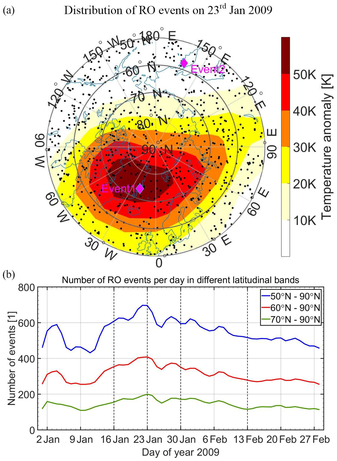
Figure 1 Illustrative distribution of RO event locations on 23 January 2009 (black dots), overplotted on the middle-stratosphere temperature anomaly of the day (a), and number of RO events per day in the latitudinal bands of 50–90^∘ N (blue), 60–90^∘ N (red), and 70–90^∘ N (green), during January and February of 2009 (b). In (a), “Event 1” represents an RO event with a large temperature anomaly, and “Event 2” one with small anomaly (diamond symbols), as used in the subsequent Figs. 2 and 3.

2.2 ECMWF analysis data

As mentioned in Sect. 1, a robust SSW definition should not only be applied to observation data, but also be readily applicable to (re)analysis and model outputs with their regular-gridded datasets. Therefore, we also use operational analysis data from the ECMWF over the same study period for a cross-check and demonstration of the applicability of our new approach also to such gridded datasets. The ECMWF analysis fields used are based on T42L91 resolution (sampled at 2.5^∘ latitude × 2.5^∘ longitude grids and 91 hybrid-pressure vertical levels up to about 80 km) and at the four time layers 00:00, 06:00, 12:00, and 18:00 UTC each day. This corresponds to roughly 300 km horizontal resolution that is similar to RO in the stratosphere (e.g., Kursinski et al., 1997). The 91 vertical levels correspond to about 1 km resolution in the tropopause region and gradually coarser resolution across the stratosphere, up to several kilometers in the mesosphere (Untch et al., 2006).

ECMWF data are used for a cross-check in two variants. The first variant is to use the RO-collocated analysis profiles, extracted by interpolation from the analysis fields to the RO event locations, together with the OPSv5.6 RO profiles. We apply the approach in the same way to these collocated analysis profiles as to the RO profiles. We note that while the density and temperature profiles derive directly from analysis field interpolations, the bending angle profiles are obtained from forward modeling (abelian transform from refractivity profiles) in the OPSv5.6 system.

The second variant is that we directly use the ECMWF analysis data at their regularly gridded resolution of 2.5^∘ × 2.5^∘, and with four time layers per day, which makes the averaging into coarser bins straightforward in this case and hence enables us to clearly assess possible (under-)sampling biases if brought in by the limited RO events' coverage, given that we intend a monitoring on a daily basis. At the same time this prepares the use of the new method with reanalysis data, such as the new European Reanalysis ERA5 (Hersbach et al., 2019, 2020; Simmons et al., 2020), foreseen in parallel to the use with RO data from over recent decades in future long-term application.

2.3 SSW detection and monitoring method

Table 1 illustrates the methodology of our SSW detection. The first step is to generate RO temperature, density, and bending angle anomaly profiles using individual RO profiles minus collocated climatological profiles, with the latter extracted from long-term gridded RO climatology fields interpolated to RO locations as described in (1), (2), and (3) of Table 1. Temperature anomalies are calculated as absolute values, while density and bending angle anomalies are calculated as relative (percentage) values, by dividing the absolute-value anomaly profiles by the collocated climatological profiles. In order to avoid the impacts of background model on bending angles, we used the non-optimized bending angle in our study. Anomalies of various atmospheric parameters have been successfully used in lots of research studies for SSW detection, cloud-top altitude detection and atmospheric blocking (Hitchcock and Shepherd, 2013; Biondi et al., 2015, 2017; Brunner et al., 2016). The long-term climatology was constructed monthly using RO data of the same months over 2007 to 2017. It is based on a 2.5^∘ latitude × 2.5^∘ longitude grid. At each of the grid centers, RO profiles within 300 km of the same month over the 11-year period are used for averaging. Sensitivity tests show that our constructed RO climatology shows only small differences to climatologies calculated using ECMWF analysis data. Based on the climatology, for our time period used as a January–February average, collocated climatological profiles can be obtained through a vertical and horizontal interpolation.

Table 1 Basic parameters and methodology of the new SSW monitoring approach (all parameters (4)–(18) updated daily; the boldfaced font in (4)–(16) shows the key parameters for the monitoring as also shown in Figs. 6 and 7).

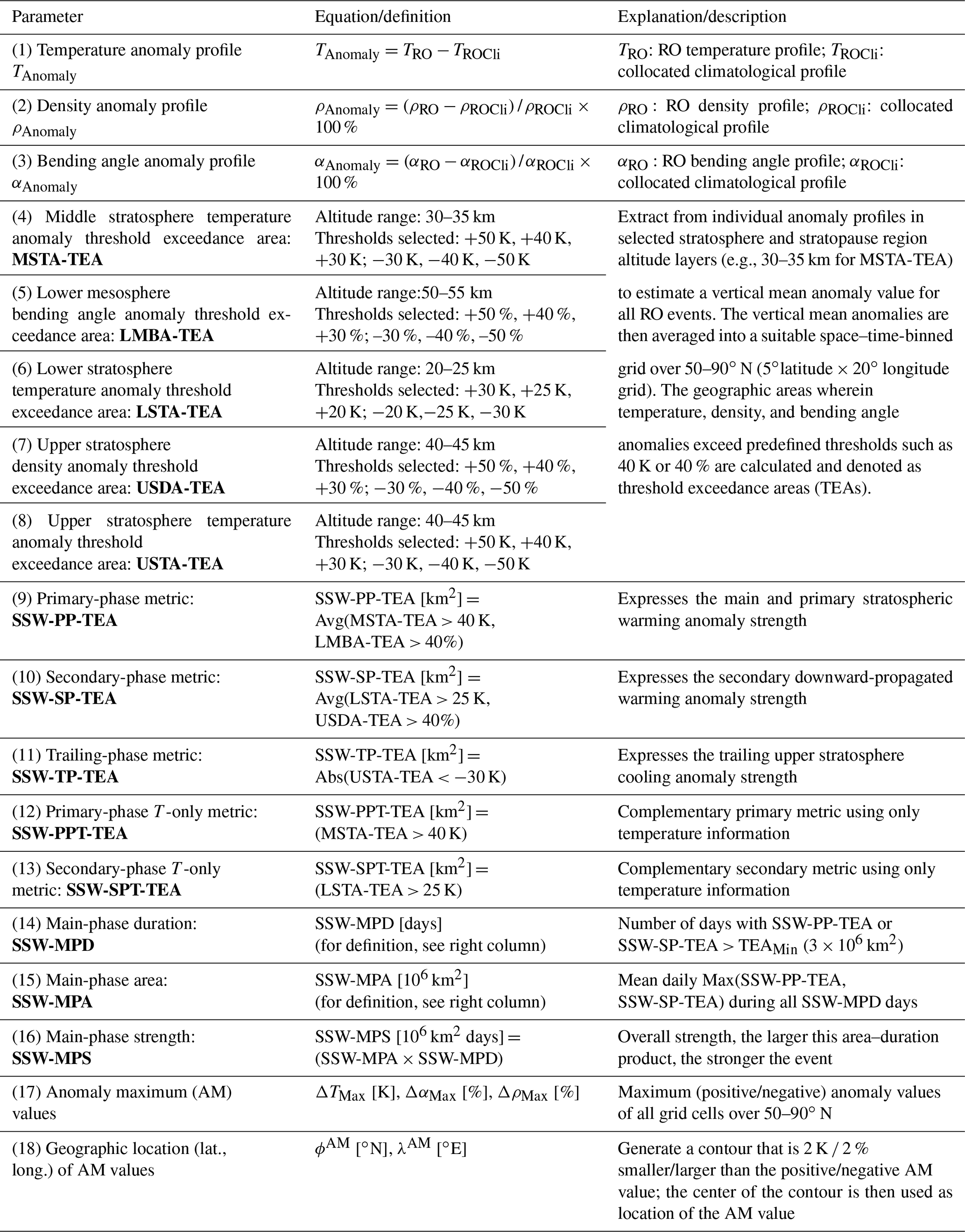
Figure 2 shows RO profiles and their anomaly profiles of two exemplary RO events as indicated in Fig. 1. Figure 2a, c, e show that RO profiles of Event 1, which is located in the area with the most warming, deviate more from climatological profiles than that of Event 2, located in an area with less warming. Anomaly profiles shown in Fig. 2b, d, f illustrate consistent larger anomalies of Event 1.

Figure 2 Event 1 and Event 2 temperature (a, b), density (c, d), and bending angle (e, f) profiles from RO and their collocated climatological profiles RO_Cli (a, c, e), together with the corresponding anomaly profiles (b, d, f), the latter computed according to Table 1, (1)–(3).

The next steps are to generate five basic daily updated thresholds exceedance areas (TEAs) as described in (4)–(8) of Table 1. The TEA is the geographic area wherein RO gridded mean anomalies of the day exceed predefined thresholds such as 40 K or  40 %. The first step of calculating the TEA is to calculate vertical mean anomaly values of selected stratospheric altitude ranges. The vertical mean anomalies are then averaged into geographic bins on a 5^∘ latitude × 20^∘ longitude grid on a daily basis over the observation area 50–90^∘ N, with grid points on latitude circles from 50 to 90^∘ N and on longitude meridians from 0 to 340^∘ E (9 × 18 grid points in total; those at 90^∘ N formally 18 points).

In order to allow for more RO events coming in, for a reliable statistical averaging, we use overlapping bin areas on the 5^∘ × 20^∘ grid as well as also including time-wise, with lower weight, the neighboring days of the given day. The latitudinal extent of the bins is set to be 10^∘ (±5^∘ about grid point latitude) for all latitude circles. Longitudinal bin extents Δλ are determined to be 30^∘ (±15^∘ about grid point longitude) at the 50^∘ N grid line and then gradually expand with increasing latitude in line with meridian convergence as $\mathrm{\Delta }{\mathit{\lambda }}_{\mathit{\phi }}=\mathrm{\Delta }{\mathit{\lambda }}_{{\mathrm{50}}^{{}^{\circ }}}\frac{\cos \left(\mathrm{50}{}^{\circ }\right)}{\cos \mathit{\phi }}$, where φ denotes the grid point latitudes from 50 to 85^∘ N. At 90^∘ N (North Pole), we just directly average data from 85^∘ N to the pole over all longitudes (and formally assign this average to all 18 grid points at 90^∘ N). The temporal extent is set to be 3 d (±1 d about given day), with the data of the 2 neighboring days getting a weight of 0.25 only, while those of the given day are weighted by 0.5. In this way, the daily sampling is indeed still meaningful, while we statistically improve the robustness of the average profiles by enabling a bigger ensemble of profiles for the weighted averaging, by taking 3 d windows. Detailed sensitivity tests showed that these selections of gridding and of spatial and temporal extents are reasonable and robust. They would allow for a more reliable statistical calculation but not blur the dynamic evolution of the SSW. Based on this averaging scheme, the number of RO profiles available per grid bin for the daily updated averaging ranges from 60 to more than 120 profiles.

To examine various atmospheric layers, five basic TEAs are calculated, i.e., MSTA-TEA (middle stratosphere temperature anomaly TEA); LMBA-TEA, (lower mesosphere bending angle anomaly TEA); LSTA-TEA (lower stratosphere temperature anomaly TEA); USDA-TEA (upper stratosphere density anomaly TEA); and USTA-TEA (upper stratosphere temperature anomaly TEA). The altitude ranges for calculating these TEAs are selected according to the response altitude ranges of the three anomalies and also the utilities of the TEAs in formulating the metrics. Response altitude ranges are regarded as the altitude ranges where anomalies show distinct increases and decreases to reflect with good sensitivity the thermodynamic changes caused by an SSW event.

Based on our inspections of small ensembles of individual RO anomaly profiles and also results of Sect. 3.1 on polar-mean anomaly profiles, the response altitude ranges for calculating the five TEAs are carefully selected according to their utilities in measuring SSW. MSTA-TEA and LMBA-TEA are used to capture the sudden warming and are therefore calculated using temperature anomalies of 30–35 km and bending angle anomalies of 50–55 km. LSTA-TEA and USDA-TEA are used to examine the downward-propagated warming, and therefore they are calculated using temperature and density anomalies in lower response altitude ranges, i.e., 20–25 km for LSTA-TEA and 40–45 km for USDA-TEA. Finally, USTA-TEA is used to capture the upper stratospheric cooling in the SSW trailing phase and is calculated using temperature anomalies of 40–45 km.

As the thresholds for calculating these five TEAs, we use those defined in Table 1, (4)–(8); for example, the thresholds for MSTA are 30, 40, and 50 K as seen therein. The selection of these thresholds was mainly guided by results on the polar-mean and regional-mean anomalies shown in Sect. 3.1 and 3.2. We examined the temporal variations of the magnitudes of warming and cooling of the five TEAs by sensitivity checks and finally chose suitable thresholds as summarized in Table 1 for the analysis of this 2009 event. Figure 3 illustrates our selection of height ranges of anomaly profiles for calculating the five TEAs based on representative example profiles. The short vertical lines represent vertical mean values in corresponding altitude ranges. For this RO event, temperature vertical mean anomalies at the 40–45, 30–35, and 20–25 km ranges are about 30, 60, and 15 K, respectively. The density vertical mean anomaly at 40–45 km is near 50 %, and the bending angle vertical mean anomaly at 50–55 km is near 70 %.

Figure 3 Temperature (blue), density (green) and bending angle (red) anomaly profiles of Event 1 (same as in Figs. 1 and 2), with the horizontal gray lines delineating the altitude layers chosen for calculating the five basic TEAs (Table 1, (4)–(8)) and the colored vertical thick lines indicating the vertical mean anomaly values in corresponding altitude layers.

Based on the five TEAs, we formulated our SSW metrics as defined in Table 1, (9)–(13), where (9)–(11) are the preferred metrics, and (12)–(13) are fallback metrics for (9)–(10), requiring only temperature as a variable. First is the SSW primary-phase metric SSW-PP-TEA (9), used to express the main and primary sudden stratospheric warming anomaly strength. It is calculated by averaging the exceedance areas MSTA-TEA > 40 K and LMBA-TEA > 40%. The secondary-phase metric SSW-SP-TEA (10) is used to express the downward-propagated warming anomaly strength and is estimated by averaging the areas LSTA-TEA > 25 K and USDA-TEA > 40%. The trailing-phase metric SSW-TP-TEA (11) expresses the trailing upper stratospheric cooling anomaly strength and is estimated using the area USTA-TEA <−30 K. The thresholds for formulating the metrics are selected based on the condition that the TEAs calculated for the chosen thresholds can suitably capture the main features of warming or cooling of the SSW event.

The preferred primary- and secondary-phase metrics (9) and (10) are constructed as a two-variable estimate (combining temperature and bending angle/density TEAs), since we find them more robust for characterizing the main phase of the SSW than single-variable metrics. However, users who prefer a simplified approach, or who only have stratospheric temperature profiles or fields available (within 20 to 45 km), can use the temperature-only metrics (12)–(13) instead, which do not include the averaging with the TEAs co-estimated from the bending angle (9) or density (10).

Based on the three metrics, either (9)–(11) or (12)–(13) and (11), we can finally detect a SSW event and monitor the strength of the event. We introduce three SSW indicators for this purpose as defined in Table 1, (14)–(16). The first is the main-phase duration, SSW-MPD, which indicates the duration of the SSW warming anomaly based on the primary- and secondary-phase metrics. This indicator is estimated by counting the number of days, with either the SSW-PP-TEA or the SSW-SP-TEA being larger than a minimum exceedance area TEA_Min. The latter is set to the plausible value of 3×10⁶ km² in this demonstration study (an area of ∼1000 km effective radius around the center location) and may become somewhat adjusted in longer term application. The second indicator is the main-phase area, SSW-MPA, which represents the mean daily threshold exceedance area during the main-phase duration. Combining these two indicators into an area–duration product yields the main-phase strength, SSW-MPS, as the third and overall indicator of the severity of the SSW, enabling a classification into weak, medium, and strong events for example.

In a follow-on work using long-term RO and reanalysis datasets, these indicators will be used to detect SSW events, for example by requiring a minimum main-phase duration of 7 d or so to qualify as an SSW and to record the strength of the events. However, the specific thresholds for our metrics and indicators for SSW detection, monitoring, and classification can only be determined after the new approach is applied to longer term data containing multiple events.

Below we demonstrate the utility to do so, both for profile-based RO and gridded analysis data, for the January–February 2009 SSW event. In addition to demonstrating the detection and monitoring approach, we also demonstrate the parallel possibility intrinsic in our TEA-based approach to dynamically track the geographic movements of any event of interest. For this purpose we introduce the parameters anomaly maximum/minimum (AM) value, and the location of these AM values, which can be used to locate the warming/cooling centers and their geographic track for the five basic TEAs. For convenience, Table 1, (17)–(18), lists and also briefly explains these auxiliary parameters.

3 Results and discussion

Section 3.1 presents temporal evolution of polar-cap mean RO anomaly profiles to have a general understanding of the characteristics of RO anomalies. Section 3.2 shows the distribution of RO gridded mean anomalies on several selected days for providing insight on the basic space–time dynamics tracked by the approach. Section 3.3 introduces our detection results of the January–February 2009 SSW demonstration event in terms of the five basic TEAs at selected thresholds and also discusses the SSW metrics of the event.

3.1 Polar-cap mean anomalies

Figure 4 shows the temporal evolution of polar-cap (60–90^∘ N) mean temperature, density, and bending angle anomaly profiles of RO data and collocated ECMWF data during the days of January and February 2009. RO temperature, density, and bending angle anomalies in their response altitude ranges show clear positive anomalies (>10 K/>10 %) from 18 January that quickly increase up to more than 30 K/40 % on 22–23 January and then quickly decrease. Such rapid increase and decrease of positive anomalies indicate a strong and rapid warming in the middle stratosphere. The positive anomalies propagate downwards to lower altitude levels (lower stratosphere for temperature, middle stratosphere for density and bending angle) and cause longer lasting anomalous conditions there till the end of February.

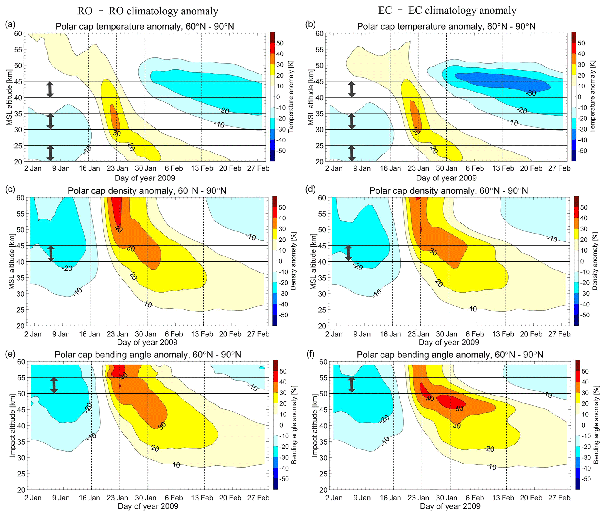
Figure 4 Temporal evolution of polar-cap (60–90^∘ N) mean temperature (a, b), density (c, d), and bending angle (e, f) anomaly profiles from RO (a, c, e), complemented by the corresponding anomalies from the ECMWF analysis data (b, d, f). The vertical dashed lines indicate 4 d selected for showing anomaly distributions in Fig. 5, and the horizontal lines in the panels delineate those altitude layers chosen for the respective variables to help compute the TEA metrics as presented in Fig. 3.

Before the sudden and rapid warming, negative anomalies are found for all the three parameters, indicating a moderate precursor cooling of the stratosphere. The cooling signal is imprinted more strongly in the density and bending angle anomalies in the upper stratosphere and lower mesosphere than observed in temperature over the lower and middle stratosphere. After the sudden warming, negative (cooling) anomalies are again found at higher altitude levels than altitude levels, showing the sudden and rapid warming, with a particular strong imprint in upper stratosphere temperature, where its fingerprint lasts many weeks, while the altitude of maximum cooling exhibits a slow downward propagation. Related to the chosen altitude layers for computing the five TEAs, we can see that they are defined so that they can capture the SSW evolution from the initial phase to the trailing phase well.

Comparing the RO-profile-based anomalies with the ECMWF-analysis-based anomalies, we find that both the magnitudes and dynamical variations of the anomalies from the two datasets are generally consistent below about 45 km. The differences are found above 45 km, where RO data show larger positive density and bending angle anomalies during the sudden warming and smaller negative temperature anomalies compared to ECMWF data, from early February after the sudden warming. These increased differences are attributable to both datasets for the following reasons: (1) ECMWF data are of sparse vertical resolution and with limited constraint from assimilated data above 50 km (e.g., Untch et al., 2006; Simmons et al., 2020), degrading their accuracy; (2) RO data accuracy reaches a somewhat higher level in bending angle and density profiles (errors < 1 % to about 50–60 km) and a lower level in temperature (<1 % to about 40 km) (e.g., Steiner et al. 2020), so that also for these data the accuracy degrades above 45 km. In the follow-on work using long-term datasets with a range of SSW events, we will analyze the different qualities of RO and (re)analysis datasets more closely, including for different RO processing and (re)analysis variants.

3.2 Spatial and temporal variations of RO anomalies

Figure 5 shows distributions of MSTA, USDA, and USTA anomalies over 50–90^∘ N on the 4 exemplary days of 16, 23, and 30 January and 13 February 2009, depicting the space–time dynamics of the SSW event during different phases of its evolution.

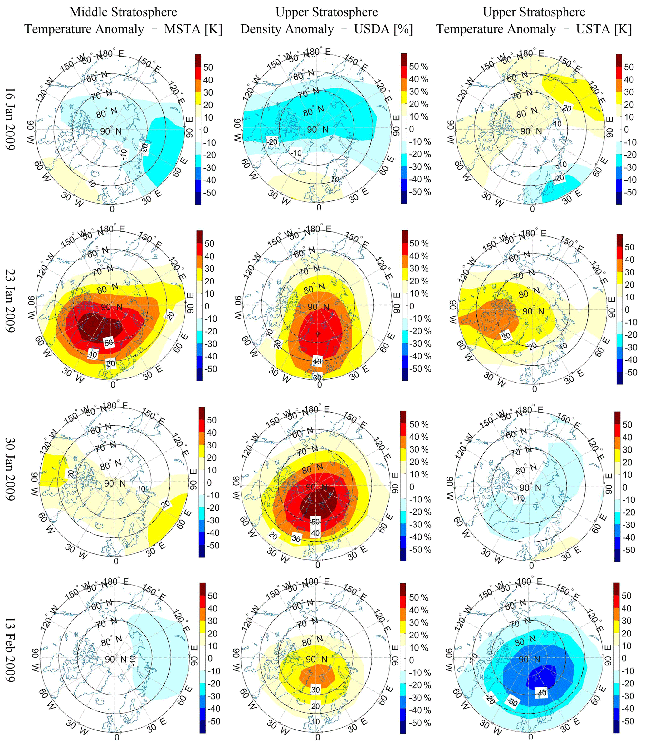
Figure 5 Middle stratosphere temperature anomaly (MSTA; left column), upper stratosphere density anomaly (USDA; middle column), and upper stratosphere temperature anomaly (USTA; right column) on the 4 exemplary days of 16, 23, and 30 January and 13 February 2009, illustrating the space–time dynamics of the SSW event in these three anomaly quantities.

Looking at MSTA results, temperature anomalies are generally negative in most of the regions on 16 January, with values up to near −30 K. Positive anomalies emerge over the northern part of the Atlantic Ocean (0–60^∘ W, 50–55^∘ N). From that day on, positive anomalies move towards higher latitudinal regions (this can be seen from map results of other days not shown here and from tracking of TEA AM values discussed in Sect. 3.3 below). The magnitudes of the anomalies increase, and the area of warming enlarges during the week after. This indicates an increase of the strength of the warming.

On 23 January, positive MSTA values dominate the whole polar-cap region across the Atlantic sector, from over North America to over Europe. The warmest region is found centered on Greenland, with anomalies exceeding 50 K. Results in this section (and in Sect. 3.3 below) indicate that 23 January 2009 is the warmest day of this SSW event. With the further progression of time, positive anomalies decrease, indicating a decrease of the strength of the warming. On 30 January, smaller anomalies of up to 20 K are found. On 13 February, which is 3 weeks after the warmest day, negative anomalies of up to −10 K are found. Results of the LMBA (not shown) confirm that variations of bending angle anomalies are generally consistent with temperature anomalies, confirming the capability of the RO bending angle to serve as a valuable support variable for monitoring SSWs, since this RO variable is observed accurately to better than 1 % up to about 60 km altitude (see Sect. 3.1).

USDA results, which are well suited to capturing the downward-propagated positive anomalies, show largest anomalies at the end of January. The warmest region is found from over eastern Greenland to oceanic regions north of Russia. On 13 February, large positive anomalies still occupy most of the polar region, indicating a long-lasting warming effect caused by the SSW. The USTA results show positive (warming) anomalies on the initial 2 d illustrated. However, on 30 January, cooling anomalies are found to occupy most of the polar region. On 13 February, the magnitude of the cooling anomalies increases to more than −40 K, and the area of strong cooling is enlarged. This indicates a strong upper stratospheric cooling, with maximum cooling centered over the oceanic part north of Russia.

3.3 SSW detection and monitoring results

Figure 6 shows the temporal evolution of the MSTA-TEA, LMBA-TEA, LSTA-TEA, USDA-TEA, and USTA-TEA results that instructively exhibit the threshold exceedance area changes during the SSW event. The geographic tracking of maximum (positive and negative) anomaly (AM) values is also shown. MSTA-TEA and LMBA-TEA results (first two rows) are generally of similar characteristics, with positive anomalies emerging from 17/18 January, which then quickly increase to maximum values on 22/23 January. MSTA-TEAs are found to be largest on 22 January, amounting for threshold exceedance areas over 30, 40, and 50 K to 20, 10, and 5×10⁶ km², respectively. LMBA-TEA values are found to be largest on 23 January, with areas exceeding the 30 %, 40 %, and 50 % thresholds, amounting to 20, 15, and 10×10⁶ km².

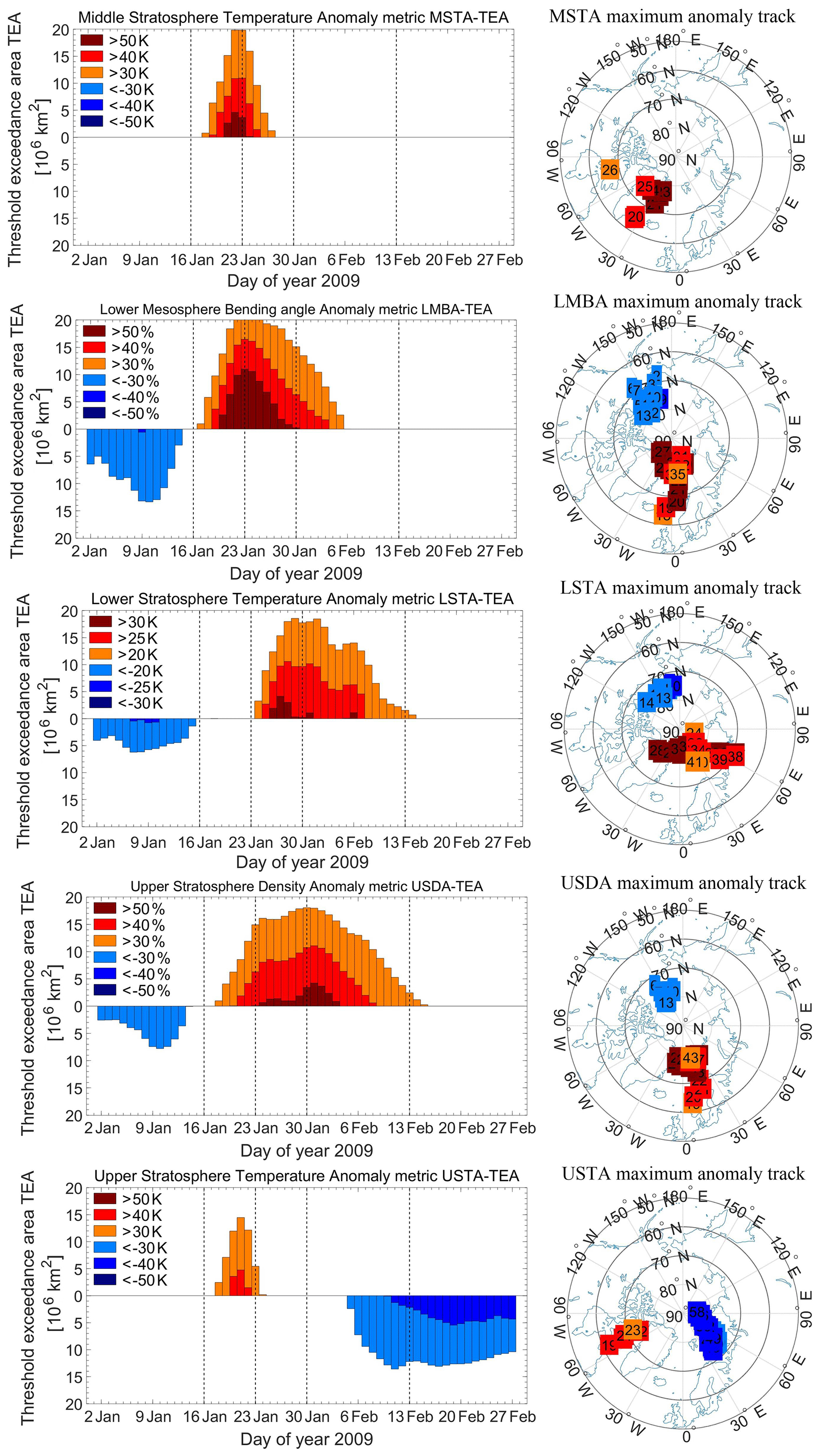
Figure 6 Time evolution of the daily MSTA, LMBA, LSTA, USDA, and USTA (from top to bottom) threshold exceedance areas (TEAs) during the SSW event, using thresholds according to Table 1, (4)–(8) (left column). For complementary space–time dynamics information, geographic tracks and magnitude classes (color scheme of left panels, numbering by day of year) of maximum positive/negative anomaly values are shown for days with TEAs with smallest thresholds >3×10⁶ km² (right column).

After the maximum value day, both MSTA-TEA and LMBA-TEA quickly decrease to zero. Such quick increase and decrease of the two metrics further reflect the sudden and rapid warming character of the SSW. Before the sudden warming, LMBA exhibits negative (cooling) anomalies as a precursor signal, with the TEA exceeding −30 % amounting to about 13×10⁶ km². The negative anomalies show a tendency of increasing and reaching maximum on 10 January and then gradually decrease in approach of the beginning of the sudden warming. After the sudden warming, there is a phase of silence, where no strong positive/negative anomalies (exceeding ± 30 K $/$ %) are found. The right panels show the tracking of AM values, indicating the movement of warming and cooling centers. It can be seen that the warming was centered over the east of Greenland, covering Greenland entirely and extending from western Norway to eastern Canada. During the most warmed days, the center locations of MSTA-TEA and LMBA-TEA AM values are close.

LSTA-TEA and USDA-TEA results are generally consistent in their evolution pattern as well, with most warming days found near the end of January and early February. Compared to the sharp increase and decrease of positive anomalies of MSTA-TEA and LMBA-TEA, the increase and decrease of LSTA-TEA and USDA-TEA are smoother, with maximum warming days somewhat delayed. The numbers of days showing positive (warming) anomalies are more than for MSTA-TEA and LMBA-TEA, indicating a longer lasting warming at the lower stratospheric altitude levels. The locations of AM values of the warming anomalies are centered over northern Russia. Negative (cooling) anomalies are found from early to middle January and are strongest over the oceanic part northeast of Russia. The USTA-TEA results, finally, show strong cooling anomalies from early February throughout the month until the end of February (end of this demonstration study analysis period). From the middle to the end of February, the TEAs that exceed a cooling of −30 and −40 K amount to about 13 and 5×10⁶ km², respectively. The cooling centers are found over the oceanic part north of Russia. These results are consistent with the strong upper stratospheric cooling in the SSW trailing phase found by a range of previous studies (e.g., Manney et al., 2008; Dhaka et al., 2015; Hitchcock and Shepherd, 2013).

Figure 7 depicts the overall results for our SSW metrics that we suggest practically using for the detection and monitoring of SSW events. Geographic tracks of the metric-relevant temperature anomalies are shown as well. The first day on which the primary-phase metric SSW-PP-TEA exceeds 3×10⁶ km² is 20 January. From this day on, SSW-PP-TEA increases quickly up to a maximum on 23 January and then quickly decreases to be smaller than 3×10⁶ km² on 31 January. The secondary-phase metric SSW-SP-TEA exceeds 3×10⁶ km² as of 23 January, increases to a maximum on 31 January, and then gradually decreases to be smaller than 3×10⁶ km² on 8 February. SSW-PP-TEA and SSW-SP-TEA comprise our defined main phase, i.e., where either or both of these two metrics exceed 3×10⁶ km².

The number of days of this main phase, our defined main-phase duration SSW-MPD, is found to be 19 d for this January–February 2009 demonstration event. The mean TEA over the main-phase duration, our defined main-phase area SSW-MPA, is 8.64×10⁶ km² for this event. Multiplying duration and area yields the SSW's main-phase strength SSW-MPS, amounting to 164.2×10⁶ km² days for this event. This clearly highlights that this SSW event extended over an area of near 2000 km effective radius around the center location for more than 2 weeks, a major part of the polar cap north of 50^∘ N. In line with previous studies on this particular event, and also with our recent preliminary studies on several other events, the values of main-phase duration and also of the strength indicate that this is a very strong SSW event.

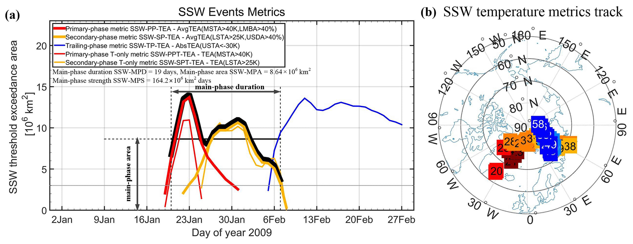
Figure 7 Time evolution of the daily primary-phase (heavy red), secondary-phase (heavy yellow), trailing-phase (light blue), primary-phase temperature-only (light red), and secondary-phase temperature-only (light yellow) metrics, respectively (a), shown for daily TEAs exceeding a TEA_Min of 3×10⁶ km² (plus a day before and after). The main-phase metrics envelope for computing the main-phase area and duration (heavy black) and the related area, duration, and strength indicator results are depicted as well (numeric results in legend), and the TEA_Min threshold is indicated (gray horizontal line). For complementary space–time dynamics information, the geographic tracks and magnitude classes of the three metric-relevant temperature anomalies (MSTA red, LSTA yellow, USTA blue) are also shown for days with TEAs > TEA_Min (b; style as in the right column of Fig. 6).

Summarizing relevant definitions, the first day of the main phase is defined as the start day of the detected event, and the end of the main phase is defined as its final day. The center day is defined as the day with a maximum TEA value of the primary metric, i.e., 23 January of this demonstration event. The trailing metric SSW-TP-TEA (blue in Fig. 7) is an auxiliary metric to capture the long-lasting upper stratospheric cooling in the wake of the event. For this January–February 2009 event, the SSW-TP-TEA exceeds 3×10⁶ km² from 6 February, then gradually increases to a maximum of near 13×10⁶ km² around middle February, and then gradually decreases to about 10×10⁶ km² at the end of the study period (end of February).

As introduced in Sect. 2.3, a simplified fallback of the approach is to use temperature as the only variable for the metric estimation. Hence we also illustrate in Fig. 7 the results for which the primary- and secondary-phase metrics are computed from temperature only (the trailing-phase metric is temperature-only anyway). These two simplified metrics are generally seen to be consistent with the preferred dual variable-based metrics, but it is visible that they appear somewhat more “volatile” and less robust in the sense that they exhibit more short-scale time variation. Follow-on work for a longer term data record with a range of SSW events will analyze these characteristics in more detail.

Figure 7b shows that the main warming tracked by SSW-PPT-TEA (red) emerges from near Iceland and extends to Greenland and moves towards higher latitudinal regions. The lower stratosphere warming (yellow/orange), tracked by SSW-SPT-TEA, is found to be emerging at the high latitudinal regions of Greenland and moving towards the northern part of Russia. The upper stratospheric cooling (blue) tracked by SSW-SPT-TEA is found to be mainly at the high latitudinal oceanic region north of Russia.

These detection and monitoring results have been cross-tested using RO-collocated profiles from ECMWF analysis and also the regularly sampled ECMWF analysis fields as alternative data sources for these datasets. The results from both datasets (not separately shown) are found to be generally consistent for this demonstration event with the detection results using RO data. This indicates that, on an individual SSW event basis, RO observational data are of comparable utility to ECMWF (re)analysis data to monitor the event, and the influence of sampling uncertainty is small. This verifies that the new approach can be readily applied to both observational and (re)analysis data (and also model output data). As discussed in the Introduction (Sect. 1), and along with the analysis data description (Sect. 2.2), follow-on work on long-term records next needs to show how the possible advantages in long-term stability and accuracy of the RO data play out or not in SSW detection and monitoring in comparison to reanalysis data.

To summarize, the metrics proposed in this study for monitoring the SSW events can satisfy the conditions well that Butler et al. (2015) suggest for proposing a standard definition (see Sect. 1). Firstly, our approach captures the sudden warming of the main phase and also its downward propagation into the lower stratosphere well, as well as the cooling occurring after the warming phase in the upper stratosphere. Secondly, the approach can be used for both RO and other suitable profile data, and likewise for reanalysis data, and can be applied for both post-processing and in real time. Finally, the new approach uses anomalies over several height layers, and TEAs over a larger area, and hence the detection and monitoring results are not sensitive to details such as exact latitude or pressure level.

Potential further refinements of the thresholds for our metrics will be determined from recently started follow-on work on multiple SSW events, using longer term data over recent decades, both from RO and reanalysis. This refinement work and testing based on a whole ensemble of SSW events with different characteristics will also complete the assessment of meeting those requirements noted by Butler et al. (2015) that relate to identifying the independence of closely timed events, the classification type (like split-type or displacement-type), and distinction of various strengths (minor, major, etc.).

4 Conclusions

In this study, we introduced a new approach to detect and monitor SSW events based on RO temperature, density, and bending angle anomaly profiles over 50–90^∘ N and demonstrated it for the well-known January–February 2009 event. The approach tracks the evolution by daily updates and is shown to be equally applicable to gridded (re)analysis data and, given the same type of gridded field structure, also to model output data.

Based on constructed anomaly profiles for the three variables temperature, density, and bending angle, we employed the concept of threshold exceedance area (TEA), which is the geographic area wherein absolute or relative anomaly values exceed predefined threshold values, as the basis for formulating SSW metrics. Computing TEAs based on anomalies in selected stratospheric altitude layers, and using adequate threshold values (mainly 40 K $/$ 40 %), we formulated three SSW detection and monitoring metrics. As a simplified fallback, the metrics can be computed alternatively from profiles or fields of temperature only.

The primary-phase metric is to examine the initial main-phase of warming caused by SSW events. The secondary-phase metric is to examine the further main phase of downward-propagated warming effects during the SSW. The trailing-phase metric is an auxiliary metric to co-examine the upper stratospheric cooling in the wake of an SSW. Based on the two main-phase metrics, we introduced three key indicators for SSW detection and monitoring. The first is the main-phase duration, recording the number of days of SSW warming that exceed a defined minimum TEA (initially set to 3×10⁶ km², corresponding to an area of about 1000 km effective radius around the center location). The second is the average daily main-phase TEA during main-phase duration, which is to quantify the average spatial extent of the event. The third is the area–duration product of the first two, termed main-phase strength, which expresses the overall strength and severity of the event.

For complementary space–time dynamics information, the approach also enables, for the selected anomaly variables, daily tracking of the maximum anomaly values and of the related geographic center location of the event. In combination with the daily TEA estimates, this also quantifies the approximate effective radius of the SSW-induced anomalies around the center location.

Applying the new approach for demonstration to the January–February 2009 SSW event, the detection and monitoring results find, where it is comparable, similar characteristics to previous studies using other approaches and datasets. We found that the SSW emerged from about 20 January and reached a maximum on 23 January and then faded by 31 January. In terms of our three indicators, the duration of the main phase of this SSW was 19 d, with an average main-phase area of 8.64×10⁶ km², yielding a main-phase strength of 164.2×10⁶ km² days. This indicates that it is a very strong SSW event, for which pronounced anomalies (>40 K $/$ >40 % >25 K) extended over an area of more than 2000 km effective radius around the center location for about 3 weeks, a major part of the polar cap north of 60^∘ N. The geographic tracking of the SSW showed that it was centered over east Greenland, covering Greenland entirely and extending from western Norway to eastern Canada. Cross-check application of the approach using ECMWF analysis data showed results generally consistent with these results from RO data. This verifies the approach to be readily applied to both irregular profile-based observational and to regular grid-based (re)analysis and model data.

Based on the encouraging demonstration in this study, follow-on work will apply the method to long-term RO and reanalysis datasets (RO overlapping 2006–2020 with reanalyses over 1979–2020) and assess its utility for long-term SSW monitoring. In this way, the most suitable settings to use for the duration, area, and overall strengths indicators for robust SSW detection, monitoring, and classification can be determined. In addition, we will be able to learn how the possible advantages in long-term stability and accuracy of the RO data play out or not in SSW monitoring in comparison to reanalysis data, including for different variants of RO processing and reanalysis. Overall, we expect the approach to be valuable for monitoring how SSW characteristics unfold event by event but also, and in particular, how they possibly vary under transient climate change and how they are in teleconnection to lower latitude regions.