Applying machine learning methods to detect convection using Geostationary Operational Environmental Satellite-16 (GOES-16) advanced baseline imager (ABI) data

An ability to accurately detect convective regions is essential for initializing models for short-term precipitation forecasts. Radar data are commonly used to detect convection, but radars that provide high-temporal-resolution data are mostly available over land, and the quality of the data tends to degrade over mountainous regions. On the other hand, geostationary satellite data are available nearly anywhere and in near-real time. Current operational geostationary satellites, the Geostationary Operational Environmental Satellite-16 (GOES-16) and Satellite-17, provide high-spatial- and high-temporal-resolution data but only of cloud top properties; 1 min data, however, allow us to observe convection from visible and infrared data even without vertical information of the convective system. Existing detection algorithms using visible and infrared data look for static features of convective clouds such as overshooting top or lumpy cloud top surface or cloud growth that occurs over periods of 30 min to an hour. This study represents a proof of concept that artificial intelligence (AI) is able, when given high-spatial- and high-temporal-resolution data from GOES-16, to learn physical properties of convective clouds and automate the detection process.

A neural network model with convolutional layers is proposed to identify convection from the high-temporal resolution GOES-16 data. The model takes five temporal images from channel 2 (0.65 µm) and 14 (11.2 µm) as inputs and produces a map of convective regions. In order to provide products comparable to the radar products, it is trained against Multi-Radar Multi-Sensor (MRMS), which is a radar-based product that uses a rather sophisticated method to classify precipitation types. Two channels from GOES-16, each related to cloud optical depth (channel 2) and cloud top height (channel 14), are expected to best represent features of convective clouds: high reflectance, lumpy cloud top surface, and low cloud top temperature. The model has correctly learned those features of convective clouds and resulted in a reasonably low false alarm ratio (FAR) and high probability of detection (POD). However, FAR and POD can vary depending on the threshold, and a proper threshold needs to be chosen based on the purpose.

1 Introduction

Artificial intelligence (AI) is flourishing more than ever as we live in the era of big data and increased processing power. Atmospheric science, with vast quantities of satellite and model data, is not an exception. In fact, numerical weather prediction and remote sensing are ideally suited to machine learning as weather forecasts can be generated on demand, and satellite data are available around the globe (Boukabara et al., 2019). Applying machine learning to forecast models can be beneficial in many ways. It can improve computational efficiency of model physics parameterizations (Krasnopolsky et al., 2005) as well as the development of new parameterizations (O'Gorman and Dwyer, 2018; Brenowitz and Bretherton, 2018; Beucler et al., 2019; Gentine et al., 2018; Rasp et al., 2018; Krasnopolsky et al., 2013). On the other hand, applying machine learning techniques to satellite data can help overcome limitations with both pattern recognition and multi-channel information extraction.

Detecting convective regions from satellite data is of great interest as convection-resolving models begin to be applied on global scales. Historically, these models were only regional, and surface radars within dense radar networks were used. Radars are useful because of the direct relationship between radar reflectivity and precipitation rates and their ability to provide vertical information about convective systems. However, ground-based radars are not available over oceanic or mountainous regions, and radars on polar-orbiting satellites have been limited to very narrow swaths. Therefore, many studies have suggested methods for using geostationary visible and infrared imagery that has good temporal and spatial coverage.

Visible and infrared data from geostationary satellites are available nearly anywhere and in near-real time. They have provided an enormous quantity of weather data, but due to the lack of vertical information, their use in forecasting has been limited largely to providing cloud top temperature or atmospheric-motion vectors in regions without convection (Benjamin et al., 2016). Some studies have tried to identify convective regions using these sensors by finding overshooting tops (Bedka et al., 2010, 2012; Bedka and Khlopenkov, 2016) or enhanced-V features (Brunner et al., 2007). However, since not all the convective clouds have such features and never until they reach a very mature stage, some studies have tried to detect broader convective regions by using lumpy cloud top surfaces (Bedka and Khlopenkov, 2016). Studies have also looked at convective initiation by observing rapidly decreasing cloud top heights (Mecikalski et al., 2010; Sieglaff et al., 2011) but were limited by tracking problems when only 15, 30, or even just 60 min data were available.

Current operational geostationary satellites, the Geostationary Operational Environmental Satellite-R (GOES-R) series, foster the use of visible and infrared sensors in detecting convection as their spatial and temporal resolutions are much improved from their predecessors. Currently operational GOES-16 and GOES-17 carry the advanced baseline imager (ABI), whose 16 channels comprise wavelengths from visible to infrared. Data are collected every 10 min over the full disk area, 5 min over contiguous United States (CONUS), and every minute in mesoscale sectors defined by the National Weather Service as containing significant weather events. When humans look at image loops of reflectance data with such high temporal resolution, most can point at convective regions because they know from past experiences that bubbling clouds resemble bubbling pots of water that imply convective heating. A recent study by Lee et al. (2020) uses several features of convective clouds such as high reflectance, low brightness temperature (T_b), and lumpy cloud top surface to detect convection from GOES-16 data in the mesoscale sector. In their method, respective thresholds for reflectance, T_b, and lumpiness are determined empirically. Here we seek to automate the process of detecting convection using AI, which, provided with the same type of information that humans use in this decision process, might be able to learn similar strategies as humans. Thus this study applies machine learning techniques to detect convection using high-temporal-resolution visible and infrared data in the ABI.

Machine learning and in particular neural networks are emerging in many remote sensing applications for clouds (Mahajan and Fataniya, 2020). Application of neural networks has led to more use of geostationary satellite data in cloud-related products such as cloud type classification or rainfall rate estimation, which has been challenging in the past (Bankert et al., 2009; Afzali Gorooh et al., 2020; Hayatbini et al., 2019; Hirose et al., 2019). Especially using GOES-16, raining clouds are detected by Liu et al. (2019) with a deep neural network model, and radar reflectivity is estimated by Hilburn et al. (2020) using a model with convolutional layers. Spectral information from several channels in geostationary satellites has been useful to deduce cloud physics along with the spatial context that can be extracted using convolutional layers.

Machine learning techniques have recently been viewed as solving every existing problem without the need for physical insight, but in practice, physical knowledge of the system is usually essential to solve problems effectively. These properties that are associated with mature convection have temporal aspects, continuously high reflectance, and high or growing cloud top height and bubbling cloud top surface over time. Therefore, these time-evolving properties are considered when selecting and processing the input and output dataset as well as when constructing the model setup.

This study explores a machine learning model with a convolutional neural network (CNN) architecture to detect convection from GOES-16 ABI data. The model is trained using Multi-Radar Multi-Sensor (MRMS), one of the radar-based products, as outputs. After training, the model results of the validation and testing dataset are compared to examine its detection skill, and two scenes from the testing data are presented to further explore which feature of convection the model uses to detect convective regions.

Features that distinguish this work from existing work are as follows: (1) studies using machine learning with geostationary satellite data are typically designed for the goal of rainfall rate estimations or classification of various cloud types, while our goal is to detect convection so that appropriate heating can be added to initiate convection in the forecast model; (2) we feed temporal sequences of GOES-16 imagery into the neural network model to provide the algorithm with the same information a human would find useful to detect the bubbling texture in GOES-16 imagery indicative of convection; (3) we use a two-step loss function approach which makes the model's performance less sensitive to threshold choice.

2 Data

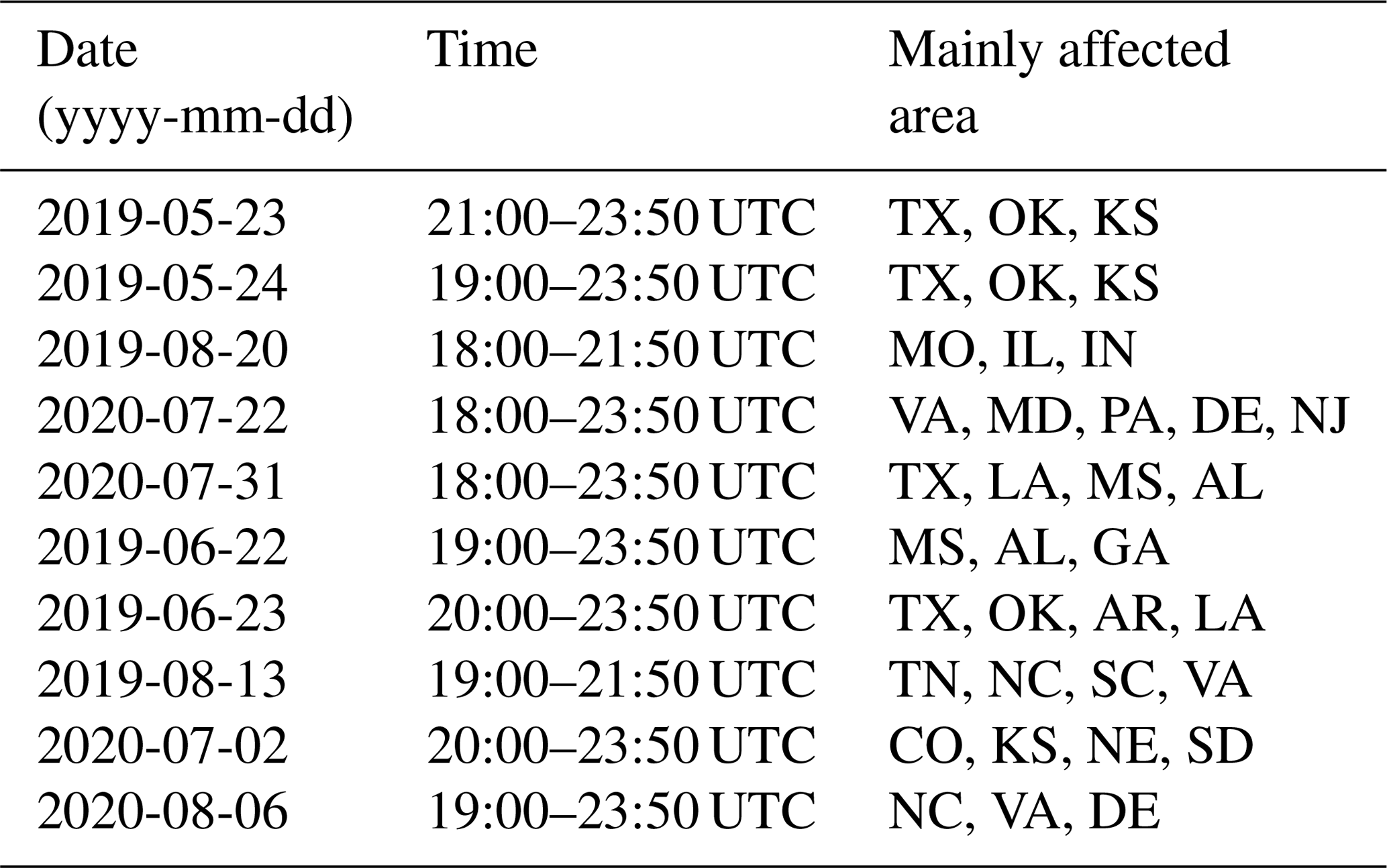
GOES-16 ABI data are used as inputs to the CNN model, while the outputs are obtained from the Multi-Radar Multi-Sensor (MRMS) dataset. Three independent datasets are prepared for training, validation, and testing. Data are collected over the central and eastern part of CONUS, where GOES-16 focuses on. Tables 1 and 2 list the time and location of 20 significant weather events to span a broad set of deep-convective storms that are used to create the dataset. Input data are obtained every 20 min so that the dataset contains the overall evolution of convection, from convective initiation to the mature stage of convection. As shown in the table, training data are selected mostly over the southern and eastern part of CONUS to effectively train the model with higher quality of radar data over those regions. A total of 19 987 training data are collected from 10 convective cases in Table 1, but only 10 019 images that contain raining scenes are used during the training, and the remaining scenes are discarded. This is done to force the model to focus more on distinguishing between the convective core and surrounding stratiform clouds rather than training with redundant non-precipitation scenes. For validation and testing, a total of 9192 and 7914 data samples are collected, respectively, each from five convective cases in Table 2. Similarly to training data, around half of both validation and testing datasets are clear regions, but no scenes are discarded in that case, whether they contain rain or not.

Table 1 A description of 10 convective cases used for training data. M1 and M2 refer to mesoscale sector 1 and 2 domain.

Table 2 A description of 10 convective cases used for validation (upper five) and testing (lower five) data.

2.1 The Geostationary Operational Environmental Satellite R series (GOES-R)

The GOES-R series, consisting of GOES-16 and GOES-17, carries the ABI with 16 channels. Channel 2 is referred to as the “red” band, and its central wavelength is at 0.65 µm. It has the finest spatial resolution, of 0.5 km, and therefore provides the most detailed image for a scene. Any data with a sun zenith angle higher than 65^∘ are removed, and reflectance data at this channel are divided by the cosine of the sun zenith angle to normalize the reflectance data. Since normalized reflectance values rarely exceed 2, any data with a reflectance value greater than 2 are truncated at 2. All data are subsequently scaled to a range from 0 to 1. Although we can observe bubbling from reflectance images on channel 2 (0.65 µm), additional T_b data can effectively remove some low cumulus clouds that appear bright. These clouds are not distinguishable from high clouds in the visible image, but they appear distinct in an infrared T_b map. Therefore, T_b data on channel 14 are also inserted as input for the AI model. Note that the spatial resolution of channel 14 is 2 km, i.e., 4 times coarser than that of channel 2. Channel 14 is a “longwave window” band, and its central wavelength is located at 11.2 µm. This channel is usually used to retrieve cloud top temperature and therefore is used to eliminate low cumulus clouds. Channel 14 data are also scaled linearly from 0 to 1, corresponding to a minimum value of 180 K and a maximum value of 320 K.

Mesoscale-sector data cover 1000 km × 1000 km domains, but the entire image is not used as an input. They are divided into smaller images to train the model more efficiently with a lower number of weights in the model and reduced clear sky regions that are not useful during training. Input data of channels 2 and 14 are created by separating the whole image into multiple 64 km × 64 km images corresponding to 128 × 128 and 32 × 32 pixels on channels 2 and 14, respectively. We refer to these small images as tiles. Each input sample then consists of five consecutive tiles on channel 2, at a 2 min interval, and five consecutive tiles on channel 14, also at a 2 min interval, but at a lower resolution.

2.2 Multi-Radar Multi-Sensor (MRMS)

MRMS data, developed at NOAA's National Severe Storms Laboratory, are produced combining radar data with atmospheric environmental data as well as satellite, lightning, and rain gauge data (Zhang et al., 2016). They have a spatial resolution of 1 km, and the data are provided every 2 min. “PrecipFlag”, one of the available variables in MRMS, classifies surface precipitation into seven categories: (1) warm stratiform rain, (2) cool stratiform rain, (3) convective rain, (4) tropical–stratiform rain mix, (5) tropical–convective rain mix, (6) hail, and (7) snow. A detailed description of the classification can be found in Zhang et al. (2016). The classification goes beyond using a simple reflectivity threshold as it considers vertically integrated liquid, composite reflectivity, and reflectivity at 0 or −10 ^∘C according to the radar's horizontal range. In addition, the quality of the product is further improved by effectively removing trailing stratiform regions with high reflectivity or regions with a bright band or melting graupel (Qi et al., 2013).

This radar-based product is used as output or truth with slight modifications. Since our model is set up to produce a binary classification of either convection or non-convection, the seven MRMS categories are reconstructed into two classes. Precipitation types of convective rain, tropical–convective rain mix, and hail are assigned as convection, and everything else is assigned as non-convection, excluding grid points with snow class. A value of either 0 (non-convective) or 1 (convective) is assigned to each grid point of the 128 × 128 tile (64 × 64 km) after applying a parallax correction with an assumed constant cloud top height of 10 km. Five MRMS data with 2 min intervals are combined to produce one output map for the model, and grid points are assigned to 1 if the grid point is assigned as convective at least once during the five time steps. In order to remove low-quality data, only the data with a “radar quality index” (RQI) greater than 0.5 are used in the study.

As mentioned in the beginning of this section, non-precipitating scenes that are not classified to any of the precipitation types are removed during training. Otherwise, the number of non-convective scenes greatly exceeds the number of convective scenes, and misclassification penalties calculated from misclassified convective cases have less of an impact on updating the model.

3 Machine learning model

The problem we are trying to solve can be interpreted as an image-to-image translation problem, namely converting the GOES-R images to a map indicating convective regions. Neural networks have been shown to be a powerful tool for this type of task. A neural network can be thought of as a function approximator that learns from a large number of input–output data pairs to emulate the mapping from input to output. Just like a linear regression model seeks to learn a linear approximation from input to output variables, neural networks seek to achieve approximations that are non-linear and might capture highly complex input–output relationships.

Convolutional neural networks (CNNs) are a special type of neural network developed for working with images, designed to extract and utilize spatial patterns in images. CNNs have different layer types that implement different types of image operations, four of which are used here, namely convolution (C), pooling (P), upsampling (U), and batch normalization (BN) layers. Convolution layers implement the type of mask and convolution operation as used in classic image processing. However, in classic image processing the masks are predefined to achieve a specific purpose, such as smoothing or edge detection, while the masks in convolutional layers have adjustable mask values that are trained to match whatever functionality is needed. Pooling layers are used to reduce the resolution of an image. For example, a so-called “maxpooling” layer of size 2 × 2 takes non-overlapping 2 × 2 patches of an image and maps each to a single pixel containing the maximum value of the 2 × 2 patch. Upsampling layers seek to invert pooling operations. For example, an upsampling layer of size 2 × 2 expands the resolution of an image by replacing each original pixel by a 2 × 2 patch through interpolation. Obviously, as information is lost in the pooling operation – an upsampling layer alone cannot invert a pooling layer – it just restores the image dimension, but additional convolution layers are needed to help fill in the remaining information. Batch normalization layers apply normalization to intermediate results in the CNN, namely enforcing constant means and variances at the input of a CNN layer, to avoid extremely large or small values, which in turn tends to speed up neural network training (Kohler et al., 2018).

The type of CNN used here is an encoder–decoder model. Encoder–decoder models take as input one or more images and feed them through sequential layers (C, P, and U) that transform the image into a series of intermediate images that finally lead to one or more images at the output. Encoder–decoder models use an encoder section with several convolution and pooling layers that reduces image dimension in order to extract spatial patterns of increasing size from the input images. The encoder is followed by a decoder section with several convolution and upsampling layers that expands the low-resolution intermediate images back into the original input image size while also expanding it in a different representation, such as converting the GOES-16 images to a map indicating convective regions.

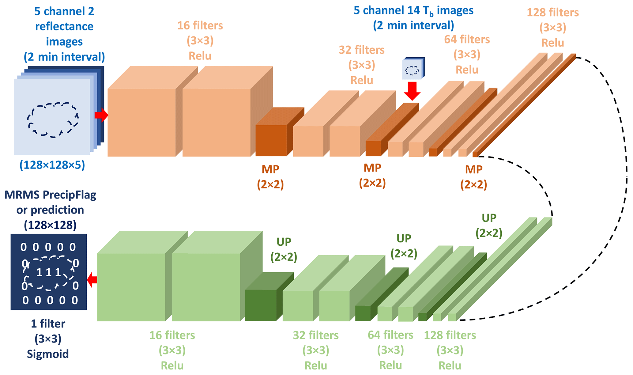
Figure 1 Description of the encoder–decoder model; 3 × 3 represents the dimensions of a filter used in convolutional layers. MP refers to the maxpooling layer, and UP refers to the upsampling layer, both with a window size of 2 × 2. Starting from five channel 2 images (upper left), the encoder section is presented in the upper row, with the additional five channel 14 images entering after the second maxpooling layer. The decoder section is shown in the lower row from right to left, with the output layer at the end (lower left).

Here an encoder–decoder model is built to produce a map of convective regions from two sets of five consecutive GOES-R images with a 2 min interval: one set from channel 2 (0.65 µm) and the other from channel 14 (11.2 µm). The encoder–decoder model is implemented using the framework of TensorFlow and Keras. Figure 1 shows the architecture of the encoder–decoder model and a model summary is shown in Table A1. Note that each convolution layer in Fig. 1 is followed by a batch normalization layer. Those batch normalization layers are not shown in Fig. 1 to keep the schematic simple but are listed in Table A1. In the input layer, only the reflectance data are read in. After two sets of two convolution layers (the first set with 16 filters and the second set with 32 filters), each set followed by a maxpooling layer, the spatial resolution of the feature maps is reduced to the same resolution as the T_b data. The T_b data are added at that point to the 32 feature maps from the previous layer, producing 37 feature maps. After another two sets of two convolution layers (each set, respectively, with 64 and 128 filters), each set followed again by one maxpooling layer, we reach the bottleneck layer of the model, i.e., the layer with the most compressed representation of the input. The bottleneck layer is the end of the encoder section of the model, and the beginning of the decoder section. The decoder section consists of four sets of two convolution layers (with a decreasing number of 128, 64, 32, and 16 filters). The first three sets of convolution layers are each followed by an upsampling layer, but the last set is followed by a transposed convolution layer with one filter to match with the 2D output. The single transposed convolution layer used here contains both upsampling and a convolution layer. Every layer uses the rectified linear unit (ReLu) activation function, except for the last transposed convolution layer, which uses a sigmoid function instead. A sigmoid function is chosen for the last layer so that the model produces a 128 × 128 map with continuous values between 0 and 1. These continuous values imply how close each pixel is to being non-convective (0) or convective (1). The values rarely reach 1, and therefore, a threshold has to be set to determine whether a grid point is convective or not. A higher threshold can increase the accuracy of the model, but more convective regions can be missed. Using different thresholds is discussed in the next section.

A neural network is trained; i.e., its parameters are optimized such that it minimizes a cost function that measures how well the model fits the data. It is very important to choose this cost function, generally called loss function for neural networks, to accurately represent the performance we want to achieve. Generally, binary cross-entropy is used for a binary classification problem, but since there is no clear boundary between convective and non-convective clouds, using a discrete value of either 0 or 1 seemed too strict, and experiments confirmed that the model did not appear to learn much when binary cross-entropy was used. Loss functions that produce continuous values are therefore used instead, resulting in continuous output values between 0 and 1, which can then (loosely) be interpreted to indicate the confidence of the neural network that a cloud is convective vs. non-convective. This approach produces better results for this application and provides additional confidence information. We investigate using a standard or two-step training approach, as described below. The standard approach minimizes a single loss function throughout the entire training. In this case, we use the mean square error (MSE) as the loss function, which penalizes misses and false alarms equally:

$$\begin{array}{}\text{(1)}& \mathrm{Loss}=\mathrm{MSE}=\sum {\left(y_{\mathrm{true}}-y_{\mathrm{predicted}}\right)}^{\mathrm{2}},\end{array}$$

where y_true is the true output image, y_predicted is the predicted output image, and the sum extends over all pixels of the true or predicted image.

The two-step training approach also starts out using the MSE as a loss function (Eq. 1). However, once the MSE on the validation data converges to a low steady value that no longer improves (which is determined by looking at the convergence plot of the loss function and the number of overlapping grid points between true and predicted convective regions as well as the sum of each true and predicted convective region), the neural network training resumes with the loss function in Eq. (2), which adds an extra penalty when the model misses convective regions (but not when it overestimates), in an effort to reduce missed regions:

$$\begin{array}{}\text{(2)}& \mathrm{Loss}=\mathrm{MSE}+\sum \mathrm{Maximum}\left(\left(y_{\mathrm{true}}-y_{\mathrm{predicted}}\right),\mathrm{0}\right),\end{array}$$

where the sum again extends over all pixels of the true/predicted image. The additional term in Eq. (2) is a positive for all pixels where the prediction is too small and 0 otherwise; thus it is expected to guide the model to detect more convective regions. The idea of using two different loss functions for coarse training and subsequent fine-tuning or, more generally, to adjust loss functions throughout different stages of training is discussed in more detail for example by Bu et al. (2020).

When using only MSE as the loss function, the model reaches convergence fairly fast after around 15 epochs, and the performance stays fairly constant after that; i.e., the model is not sensitive to the number of epochs trained beyond initial convergence. We use convergence plots, i.e., plots of loss values over epochs, to ensure each model has indeed reached this convergence. One model is trained with the standard approach (Eq. 1) and using the root mean square propagation (RMSprop) method as an optimizer (Sun, 2019) and run for 15 epochs, which shows convergence in the loss. Another model is trained with the two-step approach and the same optimizer, RMSprop. This model is first trained using MSE as the loss function (Eq. 1) for 50 epochs and then trained again using Eq. (2) for 18 epochs. In additional experiments (not shown here), similar results were obtained in the two-step approach using only 15 epochs rather than 50. A different number of epochs is used in the second model when training with MSE, but 50 is used to ensure that the model is well converged, even though the number of epochs does not matter much after 15. Results using both models are compared in the next section. Detailed evaluation of the results is only presented for the two-step approach as that represents our preferred model.

4 Results

4.1 Overall performance using a standard approach and two-step approach

In order to evaluate the detection skill of the model, the false alarm ratio (FAR), probability of detection (POD), success ratio (SR), and critical success index (CSI) are calculated for the training, validation, and testing dataset. FAR, POD, SR, and CSI can be calculated from the equations below.

$$\begin{array}{}\text{(3)}& {\displaystyle }\mathrm{FAR}={\displaystyle \frac{\mathrm{false}\mathrm{alarms}}{\mathrm{hits}+\mathrm{false}\mathrm{alarms}}}\text{(4)}& {\displaystyle }\mathrm{POD}={\displaystyle \frac{\mathrm{hits}}{\mathrm{hits}+\mathrm{misses}}}\text{(5)}& {\displaystyle }\mathrm{SR}=\mathrm{1}-\mathrm{FAR}={\displaystyle \frac{\mathrm{hits}}{\mathrm{hits}+\mathrm{false}\mathrm{alarms}}}\text{(6)}& {\displaystyle }\mathrm{CSI}={\displaystyle \frac{\mathrm{hits}}{\mathrm{hits}+\mathrm{false}\mathrm{alarms}+\mathrm{misses}}}\end{array}$$

“Hits” are grid points that are classified as convective both by the model and MRMS. Considering slight mismatch due to different views by GOES and MRMS, hits are defined for a grid point deemed convective by the CNN model if MRMS assigns convective within 2.5 km (five grid points apart) even if MRMS classifies as non-convective at the actual grid point. “Misses” are grid points that are assigned as convective by MRMS but not by the model within 2.5 km. “False alarms” are grid points that are predicted as convective by the model but not by MRMS within 2.5 km. Figure 2 shows a performance diagram (Roebber, 2009) for a model using the two-step training approach demonstrating the effect of different thresholds for the training and validation dataset. As shown in the figure, there is a trade-off between fewer false alarms and more correctly detected regions. A higher threshold prevents the model from resulting in high FAR, but at the same time, POD becomes lower, and vice versa. Compared to SR and POD of 0.86 and 0.45 from Lee et al. (2020), who use GOES-16 data as well, POD is much improved.

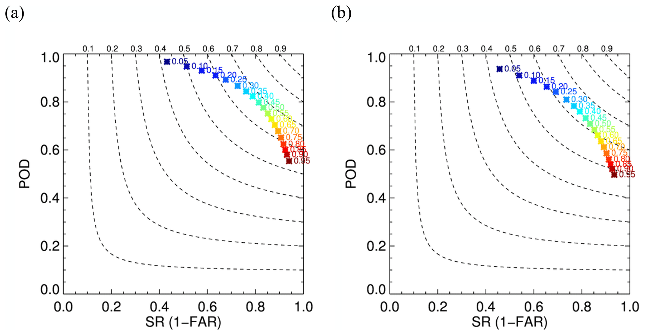
Figure 2 Performance diagrams using the two-step training approach for the (a) training and (b) testing dataset. Numbers next to the symbol are thresholds used to get corresponding SR and POD. Dashed lines represent CSI contours with labels at the top.

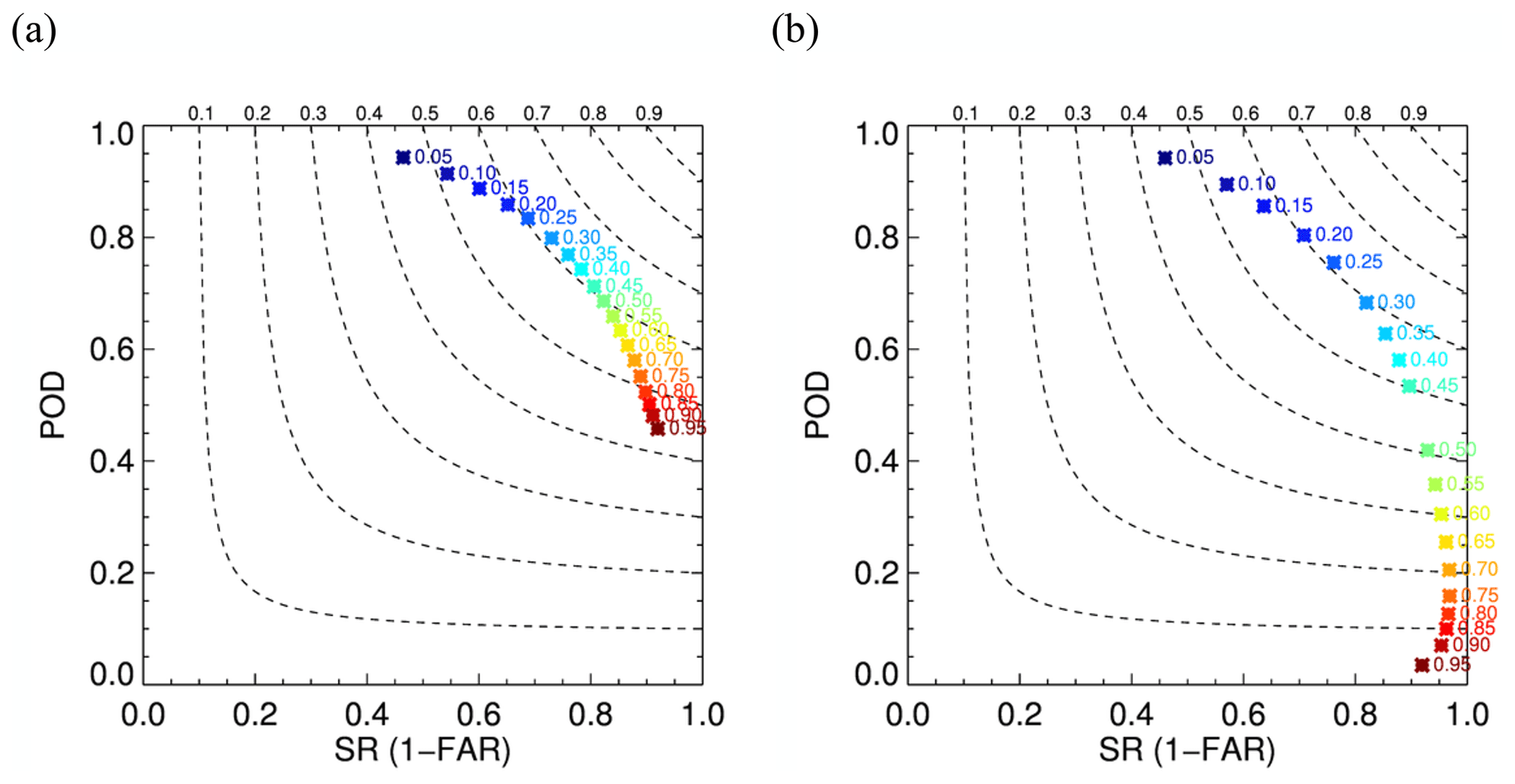
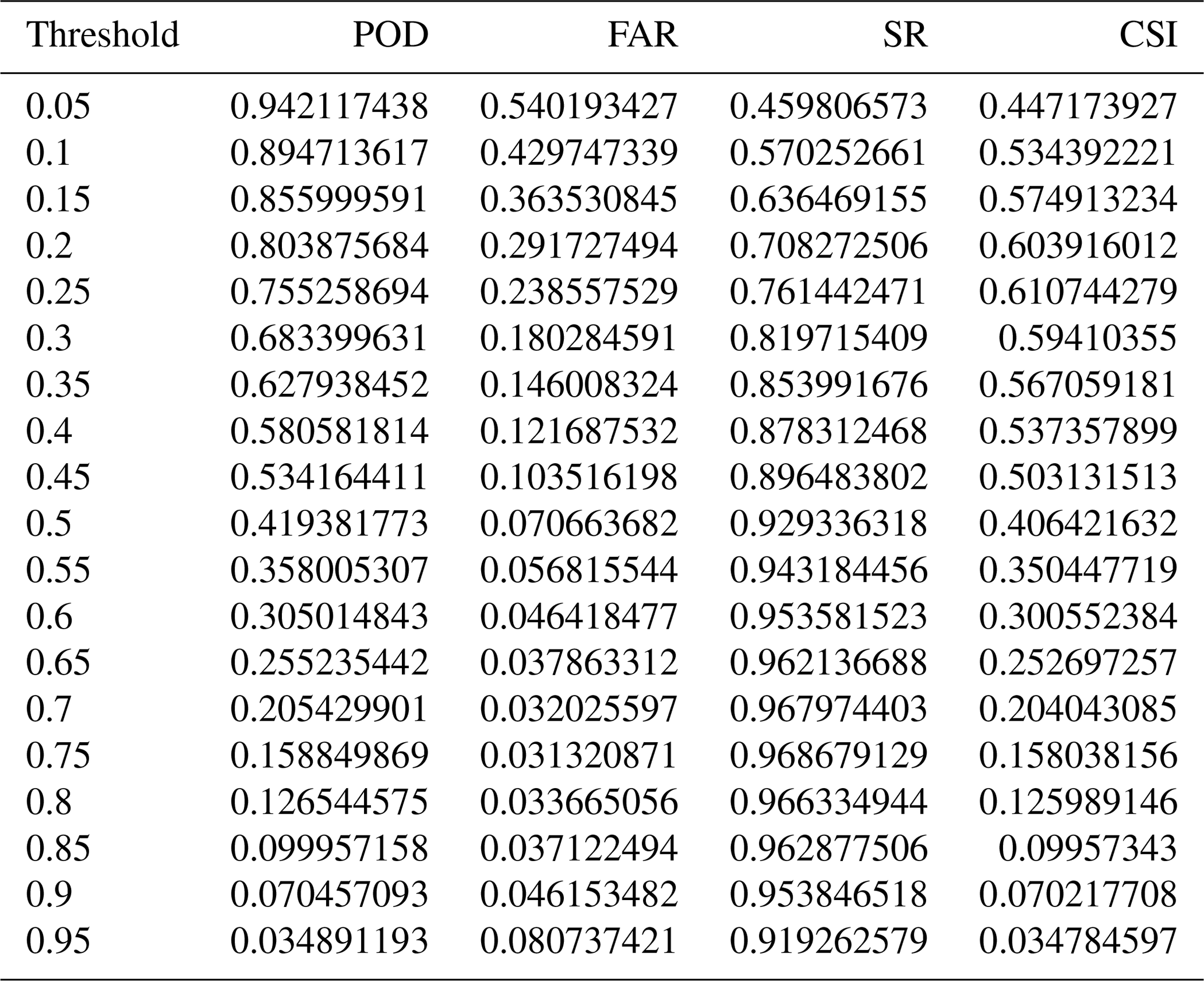
Figure 3 Performance diagrams using a model trained with the (a) two-step training approach and (b) standard approach the for testing dataset. Numbers next to the symbol are thresholds used to get corresponding SR and POD. Dashed lines represent CSI contours with labels at the top. The maximum CSI value is (a) 0.62 and (b) 0.61. CSI above 0.6 is achieved in panel (a) for thresholds from 0.25 to 0.45 and in panel (b) only for thresholds from 0.2 to 0.25. POD, FAR, SR, and CSI for all thresholds shown here are provided in Tables A2 and A3.

To compare results using the additional term in the loss function, a performance diagram for the testing dataset is shown in Fig. 3a for the same two-step model as in Fig. 2, together with a performance diagram using a model trained using the standard approach (only using MSE) in Fig. 3b. Figure 3a and b show similar curves and thus similar detection skills, but the model trained with the standard approach needs a lower threshold to achieve a similar detection skill. In Fig. 3b, SR starts to degrade as the threshold becomes higher than 0.75, indicating that grid points with higher values, which are supposed to have the highest possibility of being convective, might be falsely detected ones in the model. This effect is also observed in the two-step model for extremely large thresholds (higher than 0.95), but those are not shown in Fig. 3a. The two-step model has a slightly higher maximal CSI value, of 0.62, than the model trained with the standard approach, which has CSI of 0.61. Even though adding the second term in Eq. (2) does not seem to improve the overall detection skill significantly, the resulting two-step model has less variation in FAR and POD between the thresholds, and more thresholds in the two-step model show CSI exceeding 0.6. We thus prefer the two-step model as it delivers good performance without being overly sensitive to the specific threshold choice, so it is likely to perform more robustly across different datasets. Only results using the two-step model are further discussed.

The overall FAR and POD using the two-step approach are similar for the validation (Fig. 2b) and testing dataset (Fig. 3a), which implies that the model is consistent, but they tend to fluctuate between different convective cases. Further examination of what the model has learned to identify convection is conducted by taking a closer look at two different scenes from the testing dataset in the following subsection. For each scene, results using different thresholds are presented, and several tiles in the scene are shown for discussion.

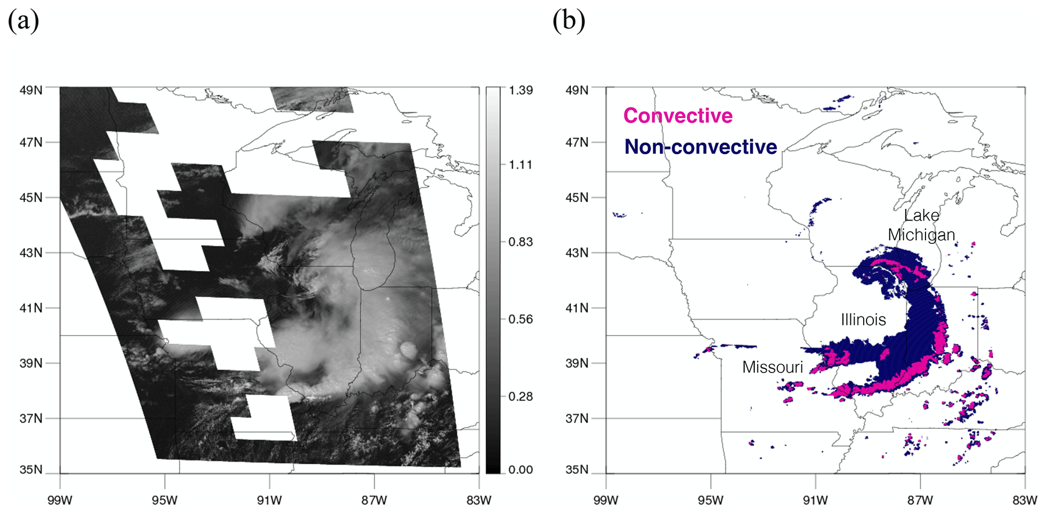
Figure 4 A scene at 19:00 UTC on 20 August 2019. (a) Visible imagery on channel 2 from GOES-16. (b) Precipitation type (convective or non-convective) classified by the MRMS PrecipFlag product. Tiles that do not appear on the map (missing square regions) are excluded due to low RQI.

Figure 5 Predicted convective regions by the model using a threshold of (a) 0.5 and (b) 0.3. Colors represent a scale of being convective (1 being convective and 0 being non-convective). The colored boxes in panel (b) indicate six scenes selected for further study, namely two scenes that are correctly identified as convection (green boxes), two scenes detected using the threshold of 0.3 but not of 0.5 (yellow boxes), and two scenes missed at both thresholds (red boxes).

4.2 Exploring results for different scenes

Figure 4a shows GOES-16 visible imagery on channel 2 on 20 August 2019 when an eastward-moving low-pressure system produced torrential rain. As described earlier, each input scene is divided into small non-overlapping tiles of 128 × 128 pixels each, as shown in Fig. 4a. Tiles with lower radar quality were eliminated from the dataset, represented as blank tiles in Fig. 4a. Each input tile is transformed separately by the neural network into an output tile of equal size and location that indicates convective and non-convective regions within the tile. These transformed tiles are then plotted in their corresponding locations, resulting in the output for an entire scene, as shown in Fig. 4b. While it is possible that the tiled approach might lead to discontinuities at tile boundaries, it does not look too discontinuous, just that sometimes a small portion of a cloud is left out in the adjacent tile, but this issue can be further improved in the future. Comparing with convective regions (pink) assigned by MRMS PrecipFlag in Fig. 4b, convective clouds in the south of Missouri and Illinois or over Indiana show clear bubbling features, while some over the Lake Michigan do not. This is reflected in the results using different thresholds as the lower threshold tends to allow less bubbling regions to be convective. FAR and POD when using 0.5 are 11.0 % and 51.4 %, while they are 15.0 % and 67.7 % with 0.3. Additional detection made by 0.3 that contributed to increase in POD mostly occurred in less bubbling regions. Convective regions predicted by the model using two different thresholds of 0.5 and 0.3 are shown in Fig. 5a and b, respectively. Colored regions in Fig. 5 are convective regions predicted by the model, and the colors represent a scale of how close it is to being convective (values close to 1 are more convective, and values close to 0 are more stratiform). It is evident from the figures that using 0.3 as the threshold detects more convective regions than using 0.5. The colored boxes in Fig. 5b indicate six scenes selected for further study, namely two scenes that are correctly identified as convection (green boxes), two scenes detected using the threshold of 0.3 but not of 0.5 (yellow boxes), and two scenes missed at both thresholds (red boxes).

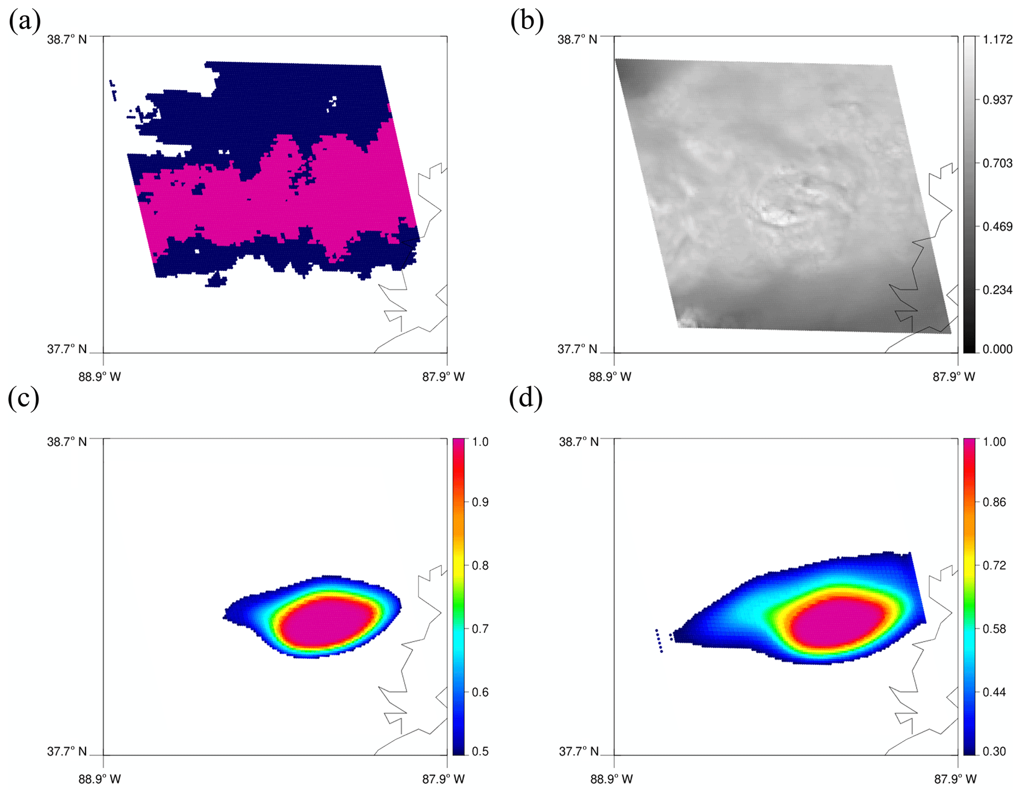
Figure 6 A 128 × 128 tile corresponding to the left yellow box in Fig. 5b. (a) MRMS PrecipFlag. (b) Reflectance on channel 2. (c) Predicted convective regions using 0.5. (d) Predicted convective regions using 0.3.

As mentioned above, the two yellow boxes in Fig. 5b are regions that are missed by the model using a threshold of 0.5 but detected by the model using 0.3. Figure 6 shows a map of MRMS PrecipFlag, reflectance, and predicted results corresponding to the 128 × 128 tile of the yellow box on the left. In Fig. 6c, some of the rainbands around 38^∘ N are missed, but they appear in Fig. 6d with the threshold of 0.3. Figure 7 shows a scene for the right yellow box. Again, more regions with less bubbling are predicted as convective with the threshold of 0.3.

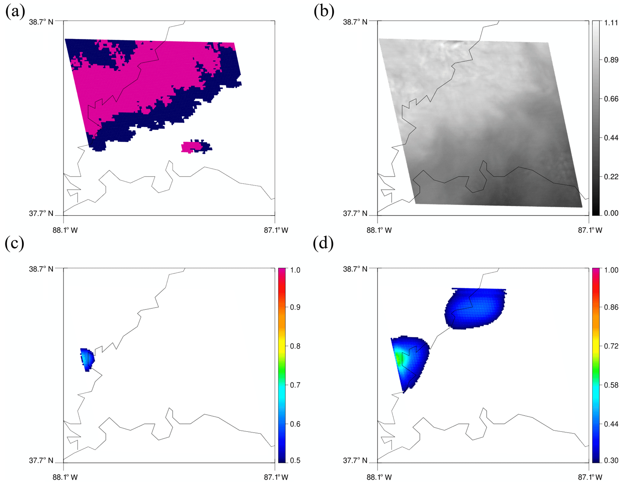
Figure 7 Same as Fig. 6 but for the right yellow box in Fig. 5b.

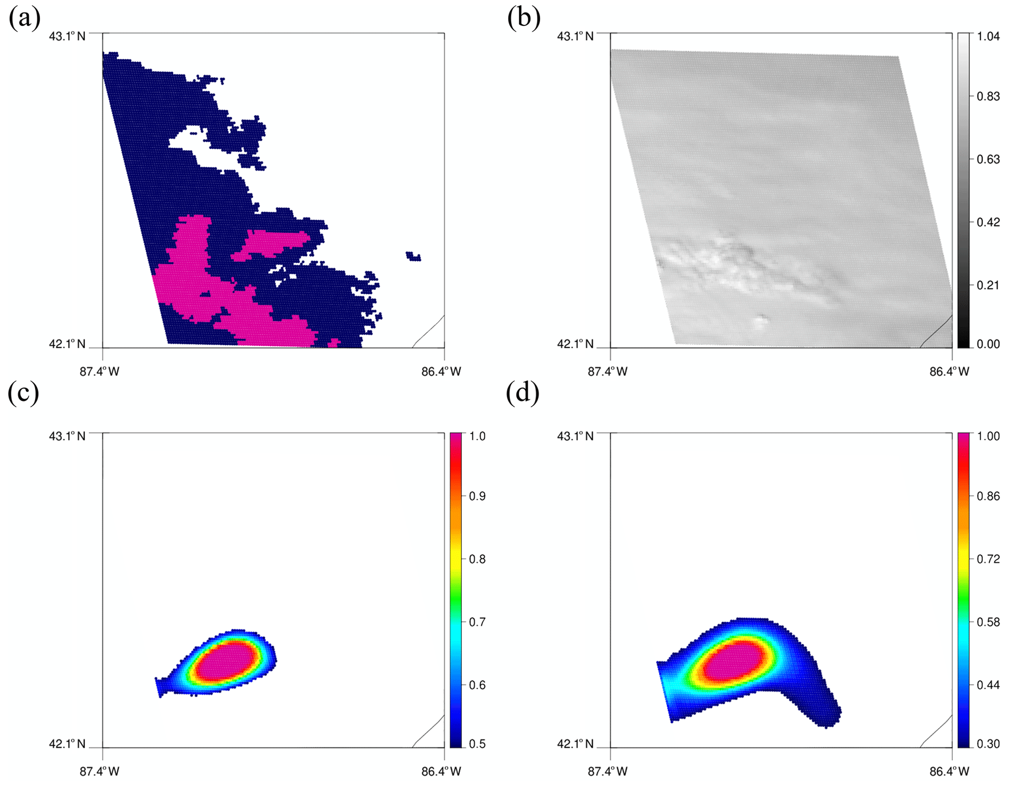
Figure 8 Same as Fig. 6 but for the upper green box in Fig. 5b.

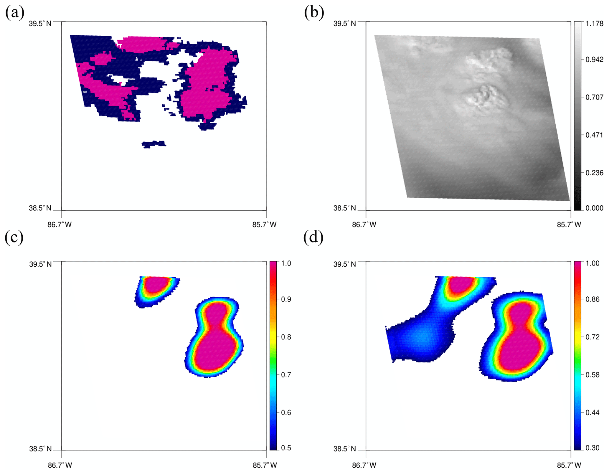
Figure 9 Same as Fig. 6 but for the lower green box in Fig. 5b.

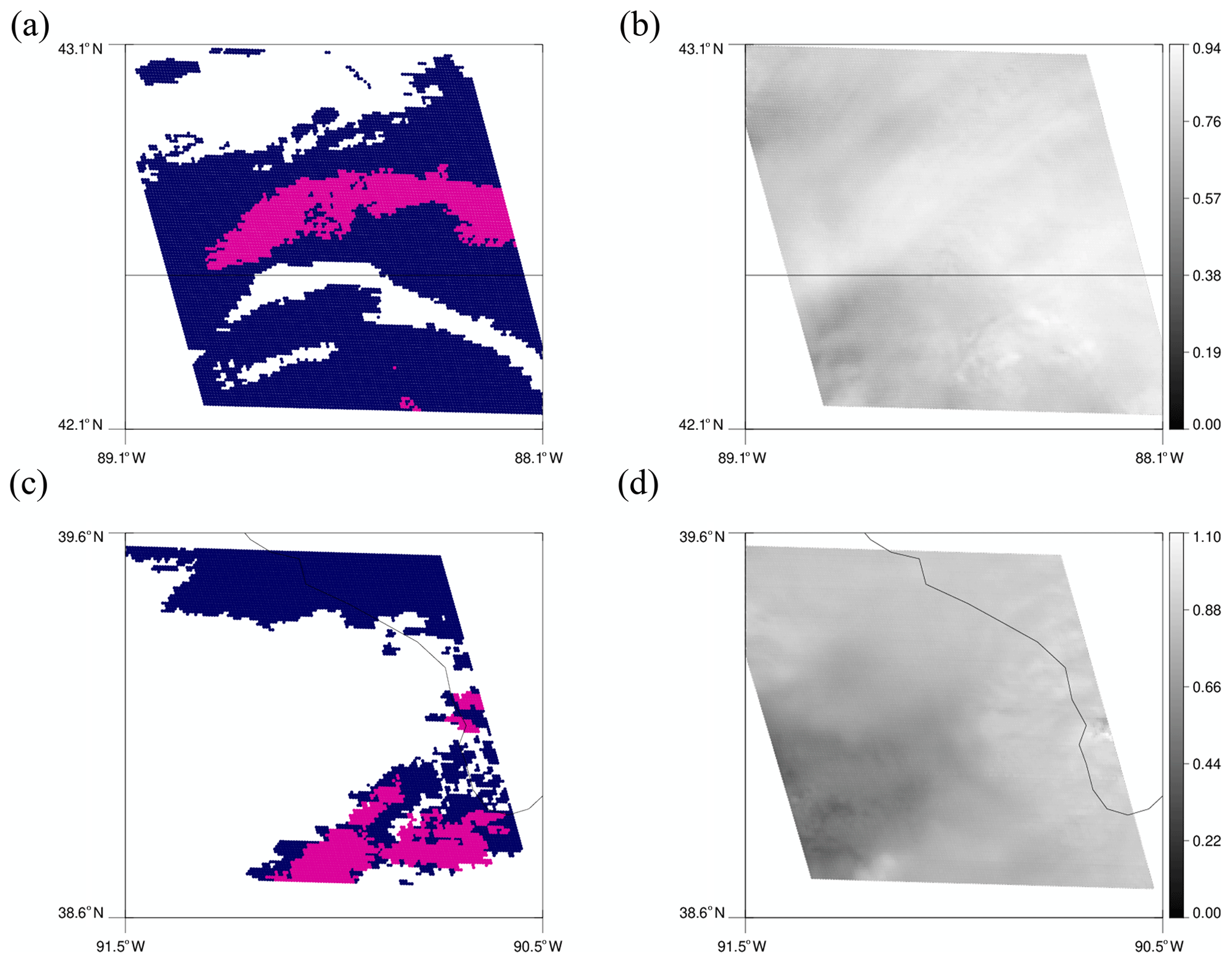
Figure 10 (a) MRMS PrecipFlag and (b) reflectance on channel 2 of the upper red box in Fig. 5b. (c) MRMS PrecipFlag and (d) reflectance on channel 2 of the lower red box in Fig. 5b.

The two green boxes in Fig. 5b are regions that are correctly predicted by the model using both thresholds. Figure 8 shows 128 × 128 tiles for the upper green box. Although the predicted regions do not perfectly align with convective regions in MRMS, each model still predicts high values in contiguous regions around the bubbling area. Convective clouds in the lower green box show clear bubbling and even overshooting top in Fig. 9b. Predicted convection using 0.5 as the threshold matches well with the bubbling regions in Fig. 9c, while using 0.3 in Fig. 9d predicts broader regions as convective. The region on the left in Fig. 9d that is additionally predicted by using 0.3 does not actually show bubbling, but MRMS also assigns it to be convective as well. Therefore, it seems that the model also learned other features that make the scene convective such as high reflectance or low T_b.

Nevertheless, some regions are still missed even with the lower threshold, and they are shown in red boxes. Figure 10a and b display MRMS PrecipFlag and the reflectance image of the 128 × 128 tile of the upper red box. While a long convective rainband is shown in the MRMS PrecipFlag, no bubbling is observed in the reflectance image even though the reflectance appears high. In addition, the lower part of convection in the lower red box (Fig. 10c and d) is also totally missed in the model prediction due to no bubbling observed in the reflectance image. These examples suggest that the model mostly looks for the bubbling feature of convective clouds to make a decision.

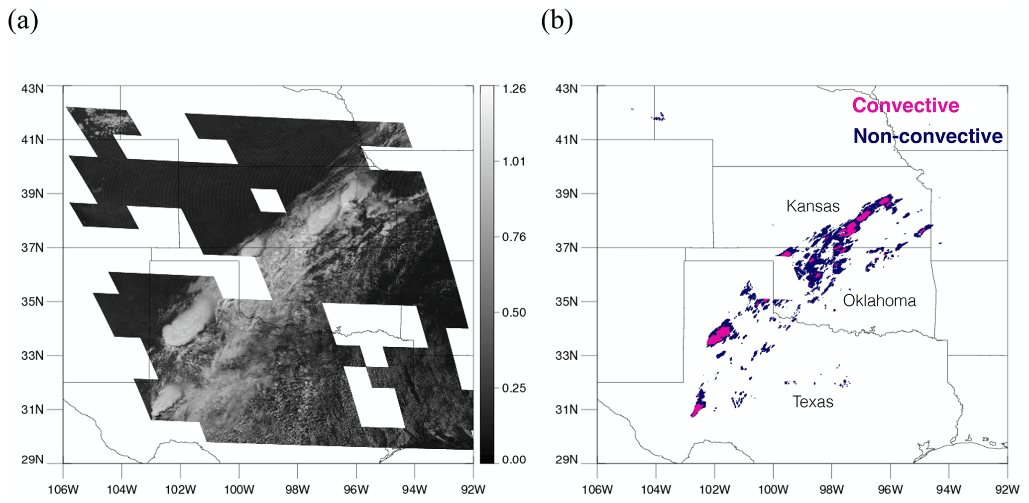
Figure 11 A scene at 19:00 UTC on 24 May 2019. (a) Visible imagery on channel 2 from GOES-16. (b) Precipitation type (convective or non-convective) classified by the MRMS PrecipFlag product. Again, tiles that do not appear on the map (missing square regions) are excluded due to low RQI.

Figure 12 Predicted convective regions by the model using a threshold of (a) 0.5 and (b) 0.3. Colors represent a scale of being convective (1 being convective and 0 being non-convective).

Another scene on 24 May 2019 is presented in Fig. 11. Severe storms occurred over Texas, Oklahoma, and Kansas, producing hail over Texas. Unlike the previous case, most convective clouds show clear bubbling, and accordingly, FAR is very low, and POD is very high in this case, even with the threshold of 0.5. With 0.5, FAR and POD are 11.0 % and 89.0 %, and they increase to 23.9 % and 95.7 % by using 0.3, respectively. More increase in FAR than in POD seems to imply that it might be wrong to use 0.3 in this case. However, the increase is mostly from detecting broader regions of mature convective clouds, and since they are farther from the convective core, sometimes they do not overlap with MRMS convective regions. In addition, earlier detection by the model than MRMS contributes to the increase. MRMS tends to define early convection as stratiform before it classifies as convective due to its low reflectivity. Convective regions in the blue boxes in Fig. 12b are such regions that did not have strong enough echoes yet to be classified as convective by MRMS, but later they are assigned as convective from 19:12 UTC once they start to produce intense precipitation. Convective regions in green boxes in Fig. 12b are additional correctly detected regions but only with the threshold of 0.3.

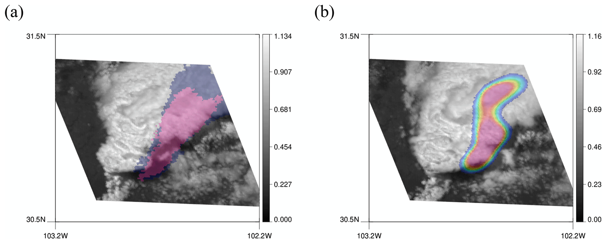
Figure 13 A 128 × 128 tile corresponding to the red box in Fig. 12a. (a) MRMS PrecipFlag on top of the first reflectance image. (b) Predicted convective regions using a threshold of 0.5 on top of the last reflectance image.

Furthermore, in some true positive cases, interesting patterns are observed. Convection in the red box in Fig. 12a is one of the true positive cases that are classified as convective by both the model and MRMS. The location of predicted convective regions matches well with MRMS. However, once the 128 × 128 tiles of MRMS and model detection are overlaid on the reflectance image, the detection area is not precisely on top of the bubbling convective core but slightly askew. In Fig. 13a and b, MRMS PrecipFlag and model prediction are plotted on top of the first and the last reflectance image, respectively, to show the temporal evolution of the convective cloud. Both MRMS and the model assign convection in the region a little to the right of the convective core and even in the dark area shadowed by the mature convective cloud. This is expected from MRMS as lumpy cloud top surfaces do not always perfectly match with precipitating location due to sheared structure of the cloud, and two instruments have different views (radar from below and satellite from above), but it is surprising that the model does predict convection in the same location as in MRMS. The model seemed to have learned about the displacement in locations and figured out where to predict convection from the radar perspective. Although it is not ideal that the prediction is not made in the bubbling area, these results can be beneficial when this product is used in the short-term forecast to initiate the convection as it resembles the radar product.

4.3 Training the model with different combinations of input variables

The model developed in this study is constructed based on the hypothesis that the high-temporal resolution data that are related to cloud properties would lead to detection of convection. Results from previous sections show that the model can predict convective regions fairly well, and thus in this section, more experiments are conducted with the same model setup but with different combinations of input variables to examine which information was most useful during training. Figure 14 shows the resulting performance diagrams. In one experiment, a model is trained using only channel 2 reflectance to assess the impact of adding channel 14 T_b (Fig. 14b). In another set of experiments, a model is trained using both channel 2 reflectance and channel 14 T_b but using only a single image (no temporal information; Fig. 14c), using two images (8 min intervals; Fig. 14d), and using three images (4 min intervals; Fig. 14e) to assess the impacts of using different-temporal-resolution data. Excluding channel 14 T_b (Fig. 14b) lowers the performance significantly compared to results in Fig. 14a (same as Fig. 3a), and using one static image (Fig. 14c) also shows a slight degradation. On the other hand, using different-temporal-resolution data in Fig. 14d and 14e shows comparable results to Fig. 14a, reaching CSI of 0.6 in some threshold cases. While no significant benefits were observed for the current neural network architecture for the highest temporal resolutions, we believe that this may be due to the relatively simple CNN architecture used here. Proposed future work includes investigation of more sophisticated neural network architectures for extracting spatio-temporal features, such as the convolutional long short-term memory (convLSTM) architecture.

Figure 14 (a) Performance diagram in Fig. 3a is shown here for ease of comparison. Performance diagrams using (b) only channel 2 reflectance images, (c) one static image, (d) two images with 8 min intervals, and (e) three images with 4 min intervals.

5 Conclusion

An encoder–decoder-type machine learning model is constructed to detect convection using GOES-16 ABI data with high spatial and temporal resolutions. The model uses five temporal images from channel 2 reflectance data and channel 14 T_b data as inputs and is trained with the MRMS PrecipFlag as outputs. Low FAR and high POD are achieved by the model, considering that they are calculated in 0.5 km resolution. However, FAR and POD can vary depending on the threshold chosen by the user. Higher POD is accompanied by higher FAR, but it was shown that some of the additional false alarms were not totally wrong because they are usually either the extension of mature convective clouds or earlier detection by the model. Earlier detection by the model actually raises the question of whether the model is well trained for early convection. If early convections were in the training dataset with a label of stratiform, then the model could learn early convective features as the feature of stratiform. However, it seemed that the model was able to correctly learn bubbling as the main feature of convection due to much larger portions of mature convective regions in the dataset.

Unlike typical objects in classic training images for image processing, e.g., cats and dogs, which have clear edges and do not change their shapes, clouds have ambiguous boundaries and varying shapes as they grow and decay. These properties of clouds make the classification problem harder. However, bubbling features of convective clouds are usually very clear in high-spatial- and high-temporal-resolution data, and the model was able to sufficiently learn the spatial context over time within the high-resolution data, which led to good detection skill. FAR and POD presented in this study are shown to be better than results applying non-machine learning methods to GOES-16 data. These results show that using GOES (or similar sensors) for identifying convective regions during the short-term forecast can be beneficial, especially over regions where radar data are not available, although this method is limited to daytime only due to the use of visible channels.

Appendix A

Table A1 Model summary of the encoder–decoder model.

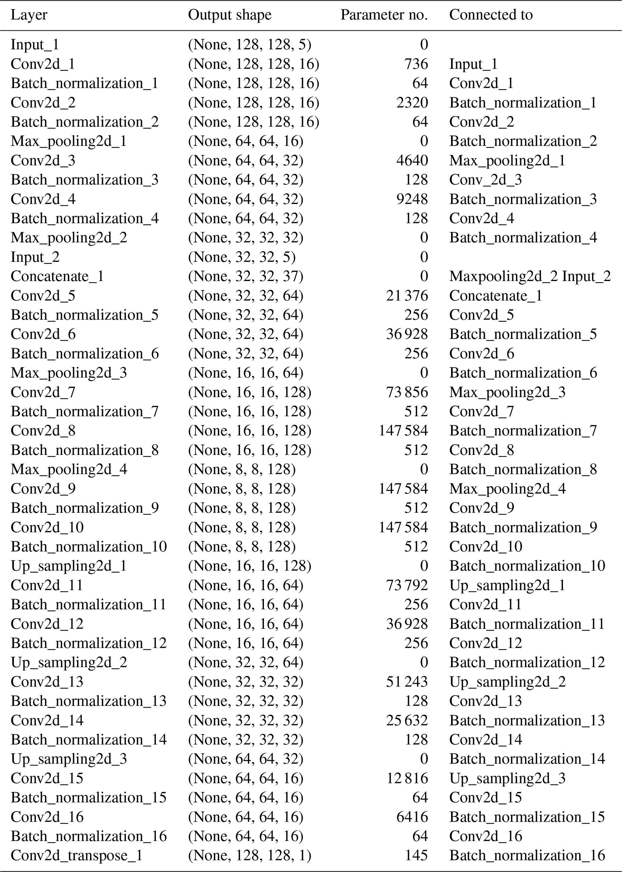
Table A2 POD, FAR, SR, and CSI values for using different thresholds in the two-step training model.

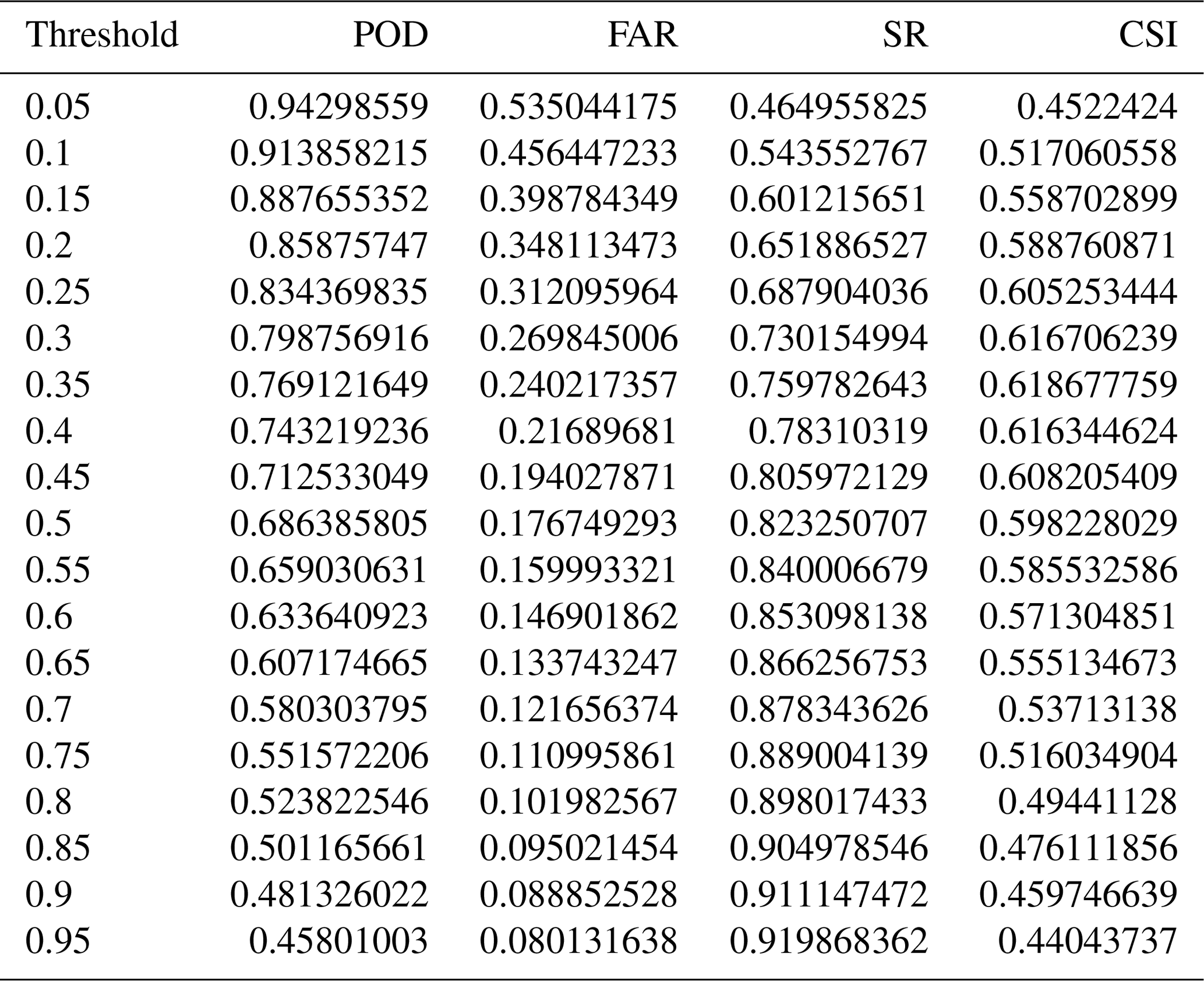
Table A3 POD, FAR, SR, and CSI values for using different thresholds in the standard training model.