the Creative Commons Attribution 4.0 License.
the Creative Commons Attribution 4.0 License.
 | 12 Apr 2021
Reducing cloud contamination in aerosol optical depth (AOD) measurements
Verena Schenzinger
Axel Kreuter
We propose a new cloud screening method for sun photometry that is designed to effectively filter thin clouds. Our method is based on a k-nearest-neighbour algorithm instead of scanning time series of aerosol optical depth. Using 10 years of data from a precision filter radiometer in Innsbruck, we compare our new method and the currently employed screening technique. We exemplify the performance of the two routines in different cloud conditions. While both algorithms agree on the classification of a data point as clear or cloudy in a majority of the cases, the new routine is found to be more effective in flagging thin clouds. We conclude that this simple method can serve as a valid alternative for cloud detection, and we discuss the generalizability to other observation sites.
- Article
(1729 KB) - Full-text XML
- BibTeX
- EndNote


Sun photometry is one of the longest-employed and robust measurement techniques for total column aerosol optical depth (AOD) retrieval (Holben et al., 1998, 2001). AOD is the most comprehensive aerosol parameter for radiative forcing studies and serves as the ground-truth for validation of satellite data. Various surface-based networks such as AERONET (Holben et al., 2001), SKYNET (Takamura and Nakajima, 2004), and the WMO Global Atmosphere Watch programme GAW-PFR (Kazadzis et al., 2018) conduct measurements of AOD at a high time resolution, providing data for local short- and long-term aerosol studies. As the calculation of AOD from photometer measurements is based on the assumption of a cloud-free path between instrument and sun, the identification and removal of cloud-contaminated data are some of the most important prerequisites for high-quality AOD data.
The most widely used algorithm by Smirnov et al. (2000) sets a threshold on the temporal variation of AOD, assuming a higher variation in the presence of clouds, as one of its flagging criteria. It was developed and employed in AERONET, as well as adapted for GAW-PFR (Kazadzis et al., 2018). While this method reliably flags thick clouds, detection of optically thin clouds exhibiting small AOD changes, i.e. below the threshold, is not possible. This limitation introduces a bias towards higher AOD (Chew et al., 2011; Huang et al., 2011), as well as a bias in the Ångström parameters, which indicate particle size.
To remedy this problem without additional manual quality control, Giles et al. (2019) revised the Smirnov et al. (2000) algorithm (see Table 2 of Giles et al., 2019, for specifics). They include aureole scans in their cloud screening routine which utilize the increased forward-scattering behaviour of thin clouds for their identification. This is suitable for instruments that measure sky radiance in addition to direct sun. However, the procedure takes time and is only viable within AERONET where these instruments are employed, whereas it is not applicable for precision filter radiometers operated within other networks, such as GAW-PFR.
Therefore, we developed a new algorithm that can identify thin clouds, and it works with direct sun measurements only. The main idea is that aerosol optical depth and microphysical properties (represented by the Ångström parameters, Gobbi et al., 2007) show little and slow variation within a day, while clouds introduce outliers and stronger fluctuations in these parameters.
Instead of scanning the time series of these variables, we examine their density in a four-dimensional space with a k-nearest-neighbour algorithm. This principle is well established in the fields of machine learning and data mining as an efficient way to identify outliers in data (Ramaswamy et al., 2000). In the context of AOD measurements, clear sky will lead to regions of high density or short distance between points, whereas clouds will result in less-dense regions or outliers.
2.1 Instrument and raw data
We use a precision filter radiometer (PFR) developed by the Physikalisch-Meteorologisches Observatorium Davos / World Radiation Center (PMOD WRC) for the GAW network (Wehrli, 2005) with four channels (368, 412, 501, 864 nm) and a field of view of 1.2∘. The instrument is set up on top of a 10-storey university building in Innsbruck, Austria (47∘15′ N, 11∘24′ E). Our operational guidelines are based on the ones of GAW, and the instrument is calibrated by PMOD. But our site runs independently of the network. In additional to the minutely (every minute) PFR reading with an acquisition time of about 2 s, we measure the air temperature and pressure at the site and monitor the overall cloud conditions with an all-sky camera taking pictures every 10 min.
2.2 Processing and filtering
First steps in quality control include the removal of data points where any of the four voltages is negative. Furthermore, flags are introduced if the sun tracker records a value higher than 15 arcsec or an ambient temperature above 310 K.
After the initial filtering, aerosol optical depth (AOD) is calculated from the voltage measurements. Starting from the Lambert–Beer law, the aerosol optical depth is derived as
where V(λ) represents the measurements, V0(λ) the calibration factors, R the Sun–Earth distance, and m the air mass in the path between instrument and sun.
Several atmospheric constituents contribute to the optical depth, one of which is aerosols (indicated by subscript a). Other factors (subscript o) which are taken into account in our calculation are Rayleigh scattering (Kasten and Young, 1989; Bodhaine et al., 1999), ozone (Komhyr et al., 1989), and NO2 (Valks et al., 2011). We use climatological values for O3 and NO2, as well as temperature and pressure measured on site. Resulting unphysical values (negative or infinite) of the aerosol optical depth at any wavelength are discarded.
At each time step, we perform a linear and a quadratic fit (indicated with subscripts l and q respectively) to τa(λ) at all four wavelengths to derive the Ångström parameters (Ångström, 1929, 1964; King and Byrne, 1976; O'Neill et al., 2001, 2003).
The spectral slope αl of the linear fit and the spectral curvature γq of the quadratic fit are used in further analysis and referred to without the subscript hereafter.
2.3 Cloud flagging
The next step in quality control of the data is the flagging of potentially cloud-contaminated data points. Figure 1 shows the basic principle of the presently employed scheme and the proposed new method.
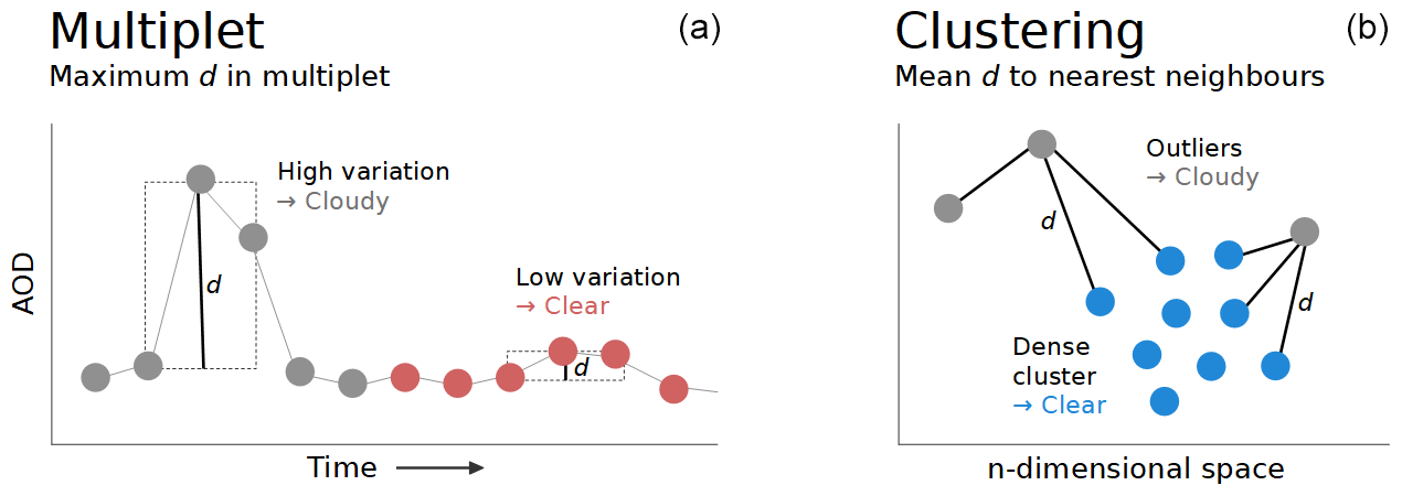
Figure 1Schematics of the cloud screening methods. (a) The Multiplet method evaluates the difference between the maximum and minimum AOD value of a set number of consecutive data points. (b) The Clustering method calculates the mean distance to k nearest neighbours in an n-dimensional space. Points for which a certain threshold of the respective measure d (indicated with the solid black lines) is passed will be identified as cloudy. These points are coloured in grey, whereas the clear points are coloured red/blue for Multiplet/Clustering.
Currently, our operational routine is based on the criteria laid out in Smirnov et al. (2000), with some minor adaptions due to the higher measurement frequency according to Wuttke et al. (2012). Data points for which the air mass exceeds a value of 6 are considered cloudy. For lower air mass, the main criterion for filtering data points is the difference between the maximum and minimum AOD value within a multiplet of consecutive data points (Smirnov et al., 2000, uses a triplet, whereas we look at a quintuplet), which cannot exceed a set value. For our site, we use a limit of 0.02 if AOD is lower than 0.2; otherwise we use 0.03. This threshold is balanced to filter clouds while retaining real AOD variations. Further limits are set on the standard deviation of AOD within a day and the second time derivative of the time series. Out of these parameters, the multiplet criterion is the most relevant (more than 99 % of the flagged points), so we will refer to the currently employed method as the “Multiplet” routine hereafter.
Instead of stepwise scanning time series, our new routine performs one calculation for all currently available data points. We use a k-nearest-neighbour algorithm to establish the 20 closest points for each of our measurements P0 in a four-dimensional space. Then the mean Euclidian distance between P0 and its neighbours is calculated (referred to as d20), and P0 is identified as cloudy if this distance exceeds a threshold. This method is usually used to identify clusters of data points; hence, we will call it the “Clustering” routine.
The dimensions used are the aerosol optical depth at 501 nm, its first derivative with respect to time, and the two Ångström parameters α and γ. The first two cover temporal variations of one wavelength, and the last two cover changes in the spectrum. To ensure that these parameters are comparable in order of magnitude (and therefore of equal weight in calculating the distance), the Ångström parameters derived from Eqs. (2) and (3) are divided by a factor of 10. Furthermore, the finite-difference time derivative of the AOD, , is used in units of 1 per 5 min (i.e. the value is divided by 12 when t is in hours), which is analogous to checking the AOD variation within a quintuplet of minutely measurements.
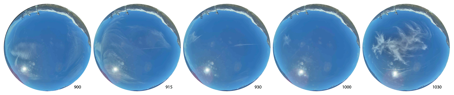
Figure 2Sky camera pictures at 15 min time resolution (time in UTC) for the time series shown in Fig. 3.
Points affected by a track error will not be considered in the set of possible nearest neighbours. If this leads to less than 20 valid measurements, the number of nearest neighbours k will be reduced accordingly down to a minimum value of 5 points in real-time analysis. To account for the lower number of nearest neighbours, the calculated distance is then multiplied by to make it comparable to the original d20 measure. Similarly, if the number of data points identified as clear on one particular day is lower than 30, the Clustering routine is rerun with 10 nearest neighbours during post-processing to ensure retention of a high number of data points.
To establish the threshold for possible cloud contamination, we calculate the distribution of d20 on about 150 clear days. We estimate a limit from this continuous distribution, which is further fine-tuned on benchmark days. These were selected as representatives of different sky conditions and examples of unidentified thin clouds by a human observer of the AOD time series, α–γ diagrams, and sky camera reference. An example (12 March 2020) is given in Figs. 2 and 3, with additional examples in Fig. A1. We show the four dimensions of our space, as well as the resulting d20 of our data points and the sky camera pictures for better illustration of the time series. Both algorithms pick up the thin clouds around 09:15 UTC, but only Clustering determines some smaller contrails between 09:30 and 10:00 as cloudy.

Figure 3Three hours of an example day (12 March 2020) to illustrate the Clustering method: time series of the four dimensions used, as well as the time series of the distance measure d20. Colour of the rectangles codes for the flagging of the data point (see legend). For the distance measure d20, points below the threshold, i.e. categorized as clear by Clustering, are coloured dark grey, and cloudy points are in light grey.
As can be seen from the d20 time series in Fig. 3, there is no clear distinction between the two states (cloudy/clear) but rather a continuous spectrum of values that has to be divided to best fit the two categories. A lower threshold value will classify the ambiguous points as cloudy but also risks a higher number of false positives and therefore lower overall data retention, which matters for error of mean values calculated from the data. Similarly, a higher threshold will cause more false negatives, i.e. cloud-contaminated points to be identified as clear. We set the d20 threshold to 0.012 considering these aspects on our clear reference and benchmark days.
To assess the performance of the Clustering routine, we will compare it to the Multiplet routine, using the last 10 years of measurements (2010–2019), with 3330 d of measurements in total. Of these days, 1906 are found to have clear data points by at least one routine.
To exemplify the similarities and differences between the two routines, Fig. 4 shows days with different cloud and aerosol conditions: clear, intermittent thick clouds, intermittent thin clouds, a combination of passing thick and thin clouds, Saharan dust, and volcanic ash. Depicted are the time series of AOD at 501 nm as well as a scatterplot of the parameters α and γ for 5 d. Additional examples are shown in Fig. A1.
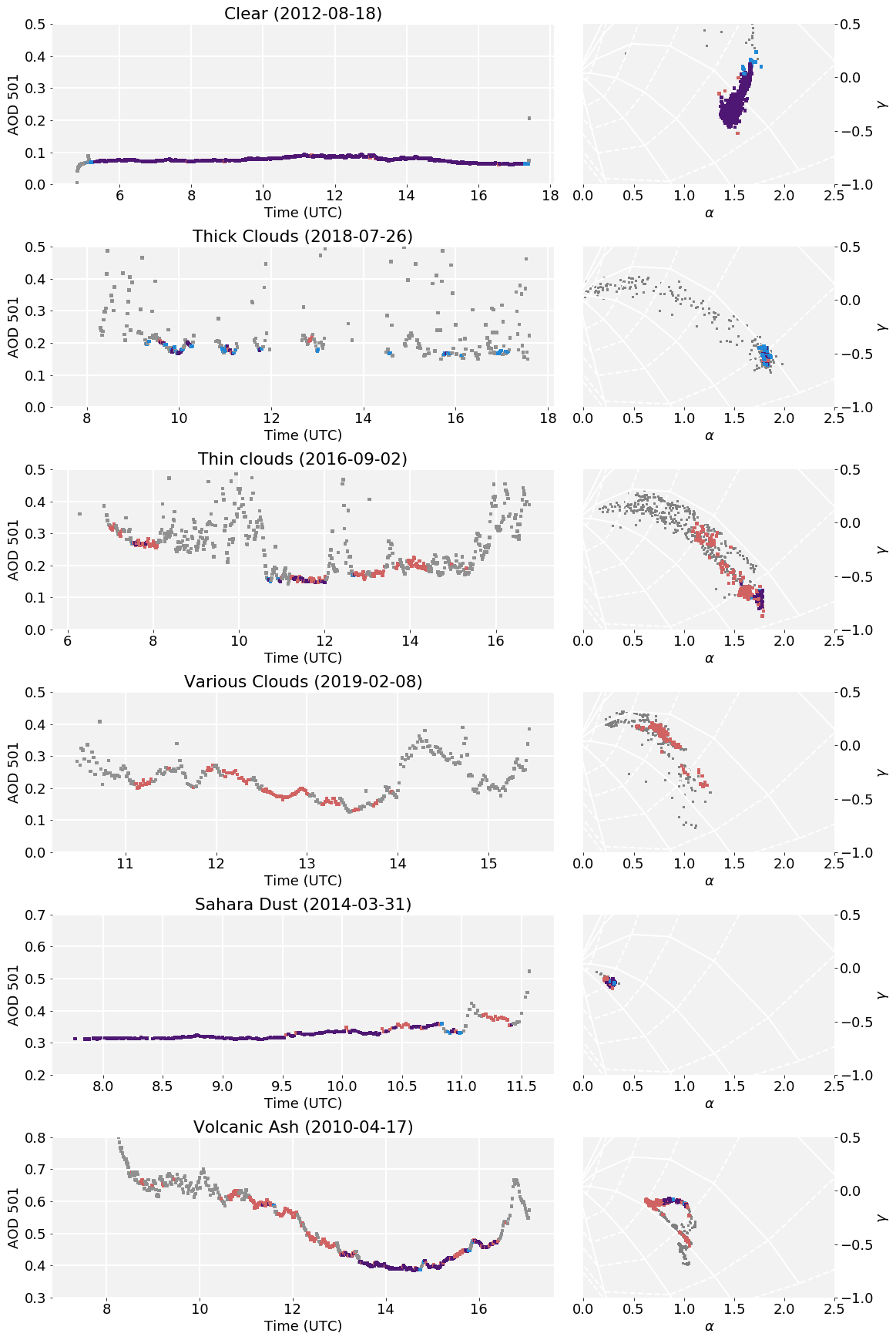
Figure 4Comparison of cloud flagging routines on selected days with different cloud conditions as signified in the respective title. Colours are as in Fig. 3. Left: time series of AOD at 501 nm, Right: α–γ plots. The solid white lines show different particle radii, and the dotted white lines show different fine mode fractions; grid adapted from Gobbi et al. (2007). Note the different x axis scales for the time series.
On a clear day, the routines agree very well, as expected. Clustering retains more points at the beginning and end of the day, which get picked up by limiting the air mass in the Multiplet routine. On the other hand, some slight outliers in α and γ get flagged by Clustering. The difference in daily mean is smaller than the measurement error.
When thick clouds are passing, with just short intervals of clear sky in between, Multiplet hardly identifies these as such. As Clustering takes all available data into account, it can assign points as clear even if the immediately preceding and consecutive point are deemed cloudy. Despite flagging less points, Clustering lowers the daily mean τ501 by 0.008 in this case, which is of similar magnitude as our measurement error.
On a day with lots of thin clouds (mainly contrails), the differences between the two routines are pronounced: a few relatively high AOD points in the morning (around 08:00 UTC) pass Clustering, as do points during midday (between 10:00 and 12:00 UTC). These points, which are spectrally very similar, are indeed cloud free, as confirmed by pictures from the sky camera. Multiplet, however, filters less points as cloudy, which show cloud contamination as a decrease in the fine mode fraction in the α–γ plane. For this day, the Clustering minus Multiplet difference of daily mean τ501 is −0.027, which is of the order of possible bias of Multiplet reported by Chew et al. (2011).
Another example of Clustering being more rigorous in cloud flagging can be seen on the day labelled with “Various Clouds”. There were several optically thick clouds passing, which get identified correctly, but neither their thin edges nor the optically thin clouds on that day get picked up by the Multiplet routine. This day gets correctly eliminated by Clustering despite Multiplet marking 89 data points as clear.
Occasionally, Saharan dust can get transported to Austria (e.g. Ansmann et al., 2003). Despite unusually high AOD, both routines correctly identify most of the data as cloud free. Daily mean τ501 is slightly lower (−0.005) when using Clustering, but this is still of the order of the calibration error.
One very unusual event is depicted last: after the eruption of Eyjafjallajökull in Iceland in April 2010, its ash plume was dispersed over Europe (Schäfer et al., 2011). It exhibits high AOD and similar particle radii and fine mode fraction as Saharan dust. Clustering flags more data due to the high variation in AOD with time but still retains data in the afternoon after about 13:00 UTC. Unfortunately, we do not have pictures available to estimate whether the data in the morning were cloud free and should therefore be retained. Clustering lowers daily mean τ501 significantly, leading to −0.057 absolute and −12 % relative difference. However, such an event is rare enough to be manually cloud screened if necessary.
Overall, the Clustering routine flags more data than the Multiplet routine, albeit not necessarily the same data points. A more detailed comparison can be seen in Fig. 5. The Multiplet routine identifies about 47.6 % of data points as cloudy and Clustering about 50.5 %, which is a realistic value considering the amount of sunshine hours Innsbruck receives on average (Stadt Innsbruck, 2019).
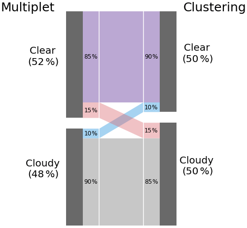
Figure 5Comparison of flagging by the two routines. The height of each area is proportional to the total number of data points in each category. Grey: both routines classify as cloudy, Red/blue/purple: Multiplet/Clustering/both classify as clear.

Figure 6Histogram of the Clustering minus Multiplet difference in daily mean of AOD at 501 nm (a) and of α (b). Negative/positive values mean that the daily mean is lower/higher when screened by Clustering.
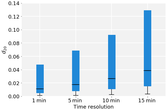
Figure 7Comparison of the distribution of d20 for different time resolutions over 10 years. The bars extend from the 25th to the 75th percentiles; the minimum and median of the distributions are indicated in black. Note that the maxima are higher than the graph range and therefore not shown.
As the main objective of the new algorithm was to filter thin clouds which previously passed the quality criteria, a higher number of flagged data points overall is expected. On the other hand, Clustering can flag isolated outliers without flagging the preceding and succeeding points of the multiplet, which lowers the number of flagged points. In 88 % of all cases, the two methods agree in the (non-)assignment of a cloud flag. Nonetheless, about 10 % of the data deemed cloudy by Multiplet are not flagged by Clustering, whereas 15 % of the data passing the Multiplet criteria are identified as cloudy by Clustering.
The mean AOD values of all clear points based on Multiplet flagging are , , , and . The respective values based on Clustering do not differ significantly, which is partly due to the low number of data points on which the routines disagree.
On daily timescales, Clustering eliminates 169 d for which Multiplet would still find valid data points. On the other hand, there are only 10 d where the opposite is the case. Nonetheless, there are more than 1000 d without clear data in the 10-year record. The number of data points on the days which are disregarded by Clustering ranges between 1 and 89. Most of these days would therefore not be considered in further analysis in other measurement networks (Kazadzis et al., 2018; Giles et al., 2019) either. Furthermore, as shown in Fig. 4, some of these days should be eliminated as they are indeed cloud contaminated.
Clustering leads to lower daily mean AOD on about 63 % of the days (Fig. 6). The mean difference is −0.0029 for , which is of the order of the calibration error (0.005 to 0.01, depending on wavelength and air mass). However, on particular days this difference can range from −0.08 to 0.04 in absolute numbers or −62 % to +27 % relative to the values based on Multiplet screening. Similarly, Clustering leads to higher mean α on 67 % of the days. Averaged over 10 years of data, this leads to an increment in by 0.02. In extreme cases, the difference can be as high as Both distributions are indicative of Clustering flagging thin clouds which Multiplet cannot properly detect.
Finally, we investigate the performance of the proposed method at lower time resolution. We subsampled the time series to 5, 10, and 15 min and analysed the resulting data with the same settings for the algorithm. Key parameters of the resulting d20 distribution from the whole 10-year data record are shown in Fig. 7. The coarser the time resolution, the higher the minimum and median d20 values and interquartile range. This is mainly due to the overall density of points decreasing, thus increasing the mean distance to the nearest neighbours. Furthermore, the values of the first time derivative will be lower, so the relative weight of this dimension decreases.
To account for the changes in density, there are two possible adjustments: lower the number of nearest neighbours or set a higher cloud flagging threshold. As an example of the latter, we show the time series on 12 March 2020 (same as in Fig. 3) at four different time resolutions in Fig. A2. With increasing the d20 threshold to 0.019, 0.027, and 0.042 respectively for 5, 10, and 15 min resolution, a very similar flagging behaviour can be achieved at all time resolutions.
We presented a new approach for flagging cloud-contaminated data points from sun photometer measurements by treating them as outliers or region of low density in a four-dimensional space. Our routine only needs one semi-empirically derived threshold and direct sun measurements for assigning a cloud flag. The method tackles shortcomings of the currently employed routine based on Smirnov et al. (2000) in the presence of optically thin clouds, such as cirrus and contrails, which lead to systematic bias of higher instant AOD values. Reducing this bias contributes to an improvement of long-term statistics and trend analysis of aerosol conditions.
While fewer data points are retained overall, which is expected from being able to filter thin clouds, the Clustering routine does not just flag more but different data points (Fig. 5). As there is an ambiguity in the transition between humidified aerosols and clouds (Koren et al., 2007), an exact discrimination between false positives and negatives for either routine is not possible. Nonetheless, the new routine leads to lower AOD and higher α in the long-term mean, which indicates a reduction of cloud contamination bias.
Detailed comparison with the previously employed cloud screening routine showed that both methods agree in their classification for the vast majority of cases (Fig. 5). Still, Clustering reduces mean AOD for most of the days in our testing period (Fig. 6). The daily mean AOD at 501 nm averaged over the last 10 years is lowered by 0.0029, which is comparable to instrument precision (Wuttke et al., 2012). However, on single days Clustering reduces daily mean by more than 0.02 (up to 0.08), which is the same magnitude as reported as bias of the Multiplet routine by Chew et al. (2011) and exceeds the error of the instrument and trace gas optical depth. Together with specific example days (Figs. 4 and A1), this supports the notion that Clustering corrects some cloudy points of the Multiplet routine to clear while flagging some of its erroneously clear points as cloudy. The small difference in the long-term mean is partly due to the specific cloud conditions in Innsbruck and could therefore be much larger in regions with higher prevalence of thin clouds.
Due to the nature of the Clustering routine, it needs at least k measurements to serve as possible nearest neighbours. In our case, we chose k=20, although dynamic adaptions can be made if there are less points available. As the accuracy of the algorithm increases with a higher number of data points, it is ideal for post-processing. Nonetheless, it can be used for real-time analysis as well, given that erroneously cloudy points can be corrected to clear when more data become available but not the other way round (i.e. points identified as clear once will be labelled as clear regardless of additional measurements).
While the four dimensions considered in the Clustering routine account for variations of one specific wavelength and in the spectrum, the question arises as to whether these can be reduced even further. Especially γ, which has the highest error of the variables (Gobbi et al., 2007), might be a candidate. Initial independence tests using mutual conditional information as a measure (Runge et al., 2019) show a strong association with α and γ. However, outliers in γ can appear independently of α, which is why we kept γ as a dimension and therefore data constraint.
So far we have tested the algorithm only for our instrument in Innsbruck. It performs well in different cloud and aerosol conditions, as shown in Fig. 4, and is able to alleviate AOD bias in the presence of thin clouds. For the application at other measurement sites, the time resolution of the data needs to be considered, as lower measurement frequency leads to lower data density and therefore higher mean distances between points (Figs. A2 and 7). Nonetheless, adaptations regarding the number of nearest neighbours, the relative weight of the different dimensions, or the d20 threshold can be easily done to optimize cloud detection with other instruments as well.
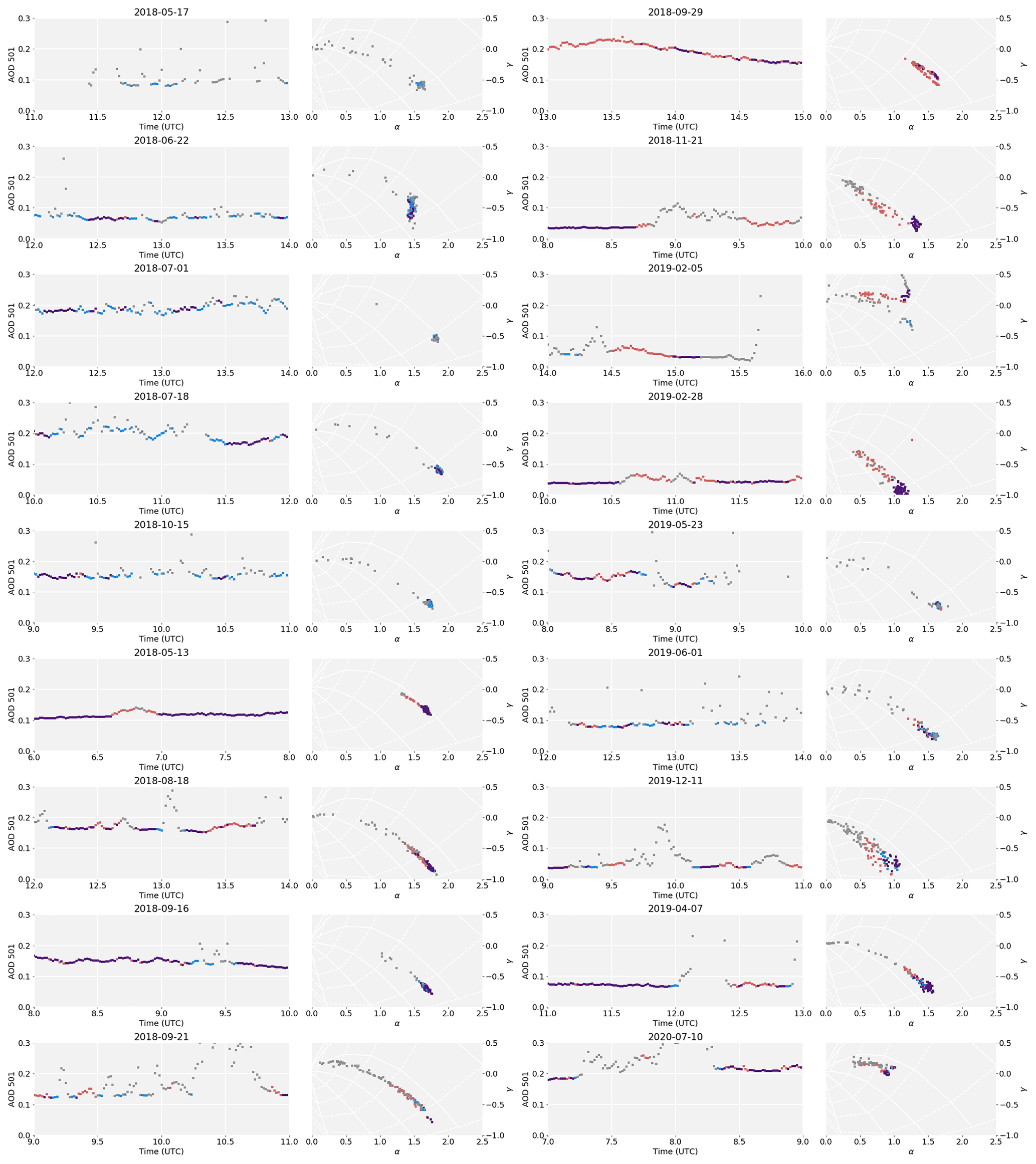
Figure A1The 2 h excerpts from selected days (in addition to Fig. 4). The first five examples highlight cases where Clustering flags much less than Multiplet; the others show the performance in the presence of thin clouds. Both categories are ordered by date.
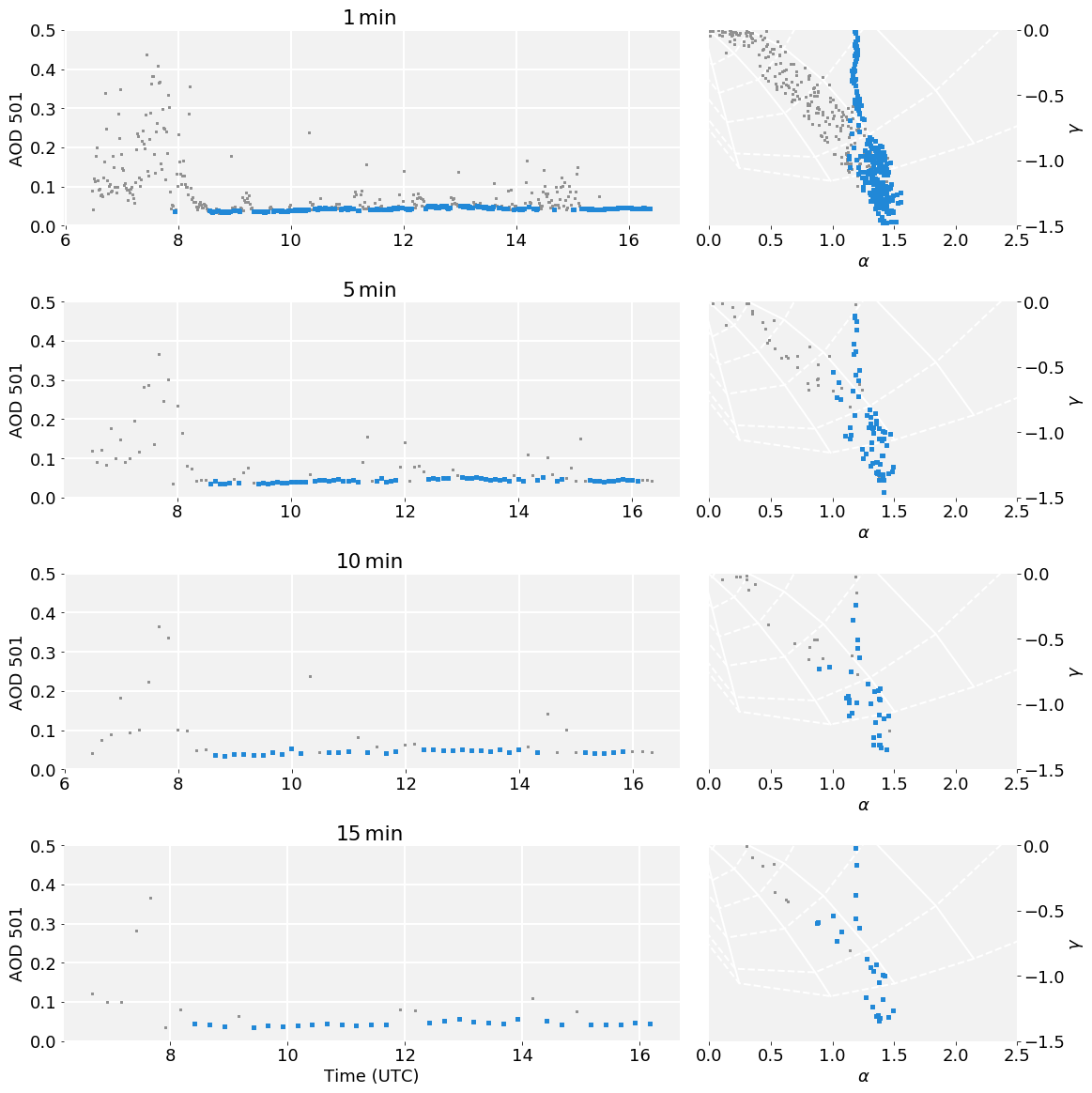
Figure A2Time series of AOD at 501 nm and α–γ plots at the original 1 min resolution, as well as 5, 10, and 15 min subsampling. Note that the initial data point was chosen randomly, so the 10 and 15 min resolutions are not a further subset of the 5 min resolution. Grey squares indicate cloudy points and blue clear ones. The cloud detection threshold was set to 0.019, 0.027, and 0.042 for the lower time resolutions.
The data and code that support the findings of this study are available from the corresponding author, Verena Schenzinger, upon request.
VS designed, implemented, and evaluated the Clustering algorithm. AK provided the raw data record. Both authors participated in writing, figure design, and interpretation of the results.
The authors declare that they have no conflict of interest.
This paper was edited by Gerd Baumgarten and reviewed by two anonymous referees.
Ångström, A.: On the Atmospheric Transmission of Sun Radiation and on Dust in the Air, Geogr. Ann., 11, 156–166, https://doi.org/10.1080/20014422.1929.11880498, 1929. a
Ångström, A.: The parameters of atmospheric turbidity, Tellus, 16, 64–75, https://doi.org/10.3402/tellusa.v16i1.8885, 1964. a
Ansmann, A., Bösenberg, J., Chaikovsky, A., Comerón, A., Eckhardt, S., Eixmann, R., Freudenthaler, V., Ginoux, P., Komguem, L., Linné, H., Márquez, M. Á. L., Matthias, V., Mattis, I., Mitev, V., Müller, D., Music, S., Nickovic, S., Pelon, J., Sauvage, L., Sobolewsky, P., Srivastava, M. K., Stohl, A., Torres, O., Vaughan, G., Wandinger, U., and Wiegner, M.: Long-range transport of Saharan dust to northern Europe: The 11–16 October 2001 outbreak observed with EARLINET, J. Geophys. Res.-Atmos., 108, 4783, https://doi.org/10.1029/2003JD003757, 2003. a
Bodhaine, B. A., Wood, N. B., Dutton, E. G., and Slusser, J. R.: On Rayleigh Optical Depth Calculations, J. Atmos. Ocean. Tech., 16, 1854–1861, https://doi.org/10.1175/1520-0426(1999)016<1854:ORODC>2.0.CO;2, 1999. a
Chew, B. N., Campbell, J. R., Reid, J. S., Giles, D. M., Welton, E. J., Salinas, S. V., and Liew, S. C.: Tropical cirrus cloud contamination in sun photometer data, Atmos. Environ., 45, 6724–6731, https://doi.org/10.1016/j.atmosenv.2011.08.017, 2011. a, b, c
Giles, D. M., Sinyuk, A., Sorokin, M. G., Schafer, J. S., Smirnov, A., Slutsker, I., Eck, T. F., Holben, B. N., Lewis, J. R., Campbell, J. R., Welton, E. J., Korkin, S. V., and Lyapustin, A. I.: Advancements in the Aerosol Robotic Network (AERONET) Version 3 database – automated near-real-time quality control algorithm with improved cloud screening for Sun photometer aerosol optical depth (AOD) measurements, Atmos. Meas. Tech., 12, 169–209, https://doi.org/10.5194/amt-12-169-2019, 2019. a, b, c
Gobbi, G. P., Kaufman, Y. J., Koren, I., and Eck, T. F.: Classification of aerosol properties derived from AERONET direct sun data, Atmos. Chem. Phys., 7, 453–458, https://doi.org/10.5194/acp-7-453-2007, 2007. a, b, c
Holben, B., Eck, T., Slutsker, I., Tanré, D., Buis, J., Setzer, A., Vermote, E., Reagan, J., Kaufman, Y., Nakajima, T., Lavenu, F., Jankowiak, I., and Smirnov, A.: AERONET – A Federated Instrument Network and Data Archive for Aerosol Characterization, Remote Sens. Environ., 66, 1–16, https://doi.org/10.1016/S0034-4257(98)00031-5, 1998. a
Holben, B. N., Tanré, D., Smirnov, A., Eck, T. F., Slutsker, I., Abuhassan, N., Newcomb, W. W., Schafer, J. S., Chatenet, B., Lavenu, F., Kaufman, Y. J., Castle, J. V., Setzer, A., Markham, B., Clark, D., Frouin, R., Halthore, R., Karneli, A., O'Neill, N. T., Pietras, C., Pinker, R. T., Voss, K., and Zibordi, G.: An emerging ground-based aerosol climatology: Aerosol optical depth from AERONET, J. Geophys. Res.-Atmos., 106, 12067–12097, https://doi.org/10.1029/2001JD900014, 2001. a, b
Huang, J., Hsu, N. C., Tsay, S.-C., Jeong, M.-J., Holben, B. N., Berkoff, T. A., and Welton, E. J.: Susceptibility of aerosol optical thickness retrievals to thin cirrus contamination during the BASE-ASIA campaign, J. Geophys. Res.-Atmos., 116, D08214, https://doi.org/10.1029/2010JD014910, 2011. a
Kasten, F. and Young, A. T.: Revised optical air mass tables and approximation formula, Appl. Optics, 28, 4735–4738, https://doi.org/10.1364/AO.28.004735, 1989. a
Kazadzis, S., Kouremeti, N., Nyeki, S., Gröbner, J., and Wehrli, C.: The World Optical Depth Research and Calibration Center (WORCC) quality assurance and quality control of GAW-PFR AOD measurements, Geosci. Instrum. Method. Data Syst., 7, 39–53, https://doi.org/10.5194/gi-7-39-2018, 2018. a, b, c
King, M. D. and Byrne, D. M.: A Method for Inferring Total Ozone Content from the Spectral Variation of Total Optical Depth Obtained with a Solar Radiometer, J. Atmos. Sci., 33, 2242–2251, https://doi.org/10.1175/1520-0469(1976)033<2242:AMFITO>2.0.CO;2, 1976. a
Komhyr, W. D., Grass, R. D., and Leonard, R. K.: Dobson spectrophotometer 83: A standard for total ozone measurements, 1962–1987, J. Geophys. Res.-Atmos., 94, 9847–9861, https://doi.org/10.1029/JD094iD07p09847, 1989. a
Koren, I., Remer, L. A., Kaufman, Y. J., Rudich, Y., and Martins, J. V.: On the twilight zone between clouds and aerosols, Geophys. Res. Lett., 34, L08805, https://doi.org/10.1029/2007GL029253, 2007. a
O'Neill, N. T., Eck, T. F., Holben, B. N., Smirnov, A., Dubovik, O., and Royer, A.: Bimodal size distribution influences on the variation of Angstrom derivatives in spectral and optical depth space, J. Geophys. Res.-Atmos., 106, 9787–9806, https://doi.org/10.1029/2000JD900245, 2001. a
O'Neill, N. T., Eck, T. F., Smirnov, A., Holben, B. N., and Thulasiraman, S.: Spectral discrimination of coarse and fine mode optical depth, J. Geophys. Res.-Atmos., 108, 4559, https://doi.org/10.1029/2002JD002975, 2003. a
Ramaswamy, S., Rastogi, R., and Shim, K.: Efficient Algorithms for Mining Outliers from Large Data Sets, SIGMOD Rec., 29, 427–438, https://doi.org/10.1145/335191.335437, 2000. a
Runge, J., Nowack, P., Kretschmer, M., Flaxman, S., and Sejdinovic, D.: Detecting and quantifying causal associations in large nonlinear time series datasets, Sci. Adv., 5, eaau4996, https://doi.org/10.1126/sciadv.aau4996, 2019. a
Schäfer, K., Thomas, W., Peters, A., Ries, L., Obleitner, F., Schnelle-Kreis, J., Birmili, W., Diemer, J., Fricke, W., Junkermann, W., Pitz, M., Emeis, S., Forkel, R., Suppan, P., Flentje, H., Gilge, S., Wichmann, H. E., Meinhardt, F., Zimmermann, R., Weinhold, K., Soentgen, J., Münkel, C., Freuer, C., and Cyrys, J.: Influences of the 2010 Eyjafjallajökull volcanic plume on air quality in the northern Alpine region, Atmos. Chem. Phys., 11, 8555–8575, https://doi.org/10.5194/acp-11-8555-2011, 2011. a
Smirnov, A., Holben, B., Eck, T., Dubovik, O., and Slutsker, I.: Cloud-Screening and Quality Control Algorithms for the AERONET Database, Remote Sens. Environ., 73, 337–349, https://doi.org/10.1016/S0034-4257(00)00109-7, 2000. a, b, c, d, e
Stadt Innsbruck: Monats- und Jahressummen der Sonnenscheindauer seit 1906, available at: https://www.innsbruck.gv.at/data.cfm?vpath=redaktion/ma_i/allgemeine_servicedienste/statistik/dokumente38/meteorologischebeobachtungen/monatsjahressonnenscheindauerseit1906pdf (last access: 25 March 2021), 2019. a
Takamura, T. and Nakajima, T.: Overview of SKYNET and its activities, Optica Pura y Aplicada, 37, 3303–3308, 2004. a
Valks, P., Pinardi, G., Richter, A., Lambert, J.-C., Hao, N., Loyola, D., Van Roozendael, M., and Emmadi, S.: Operational total and tropospheric NO2 column retrieval for GOME-2, Atmos. Meas. Tech., 4, 1491–1514, https://doi.org/10.5194/amt-4-1491-2011, 2011. a
Wehrli, C.: GAWPFR: A Network of Aerosol Optical Depth Observatioins with Precision Filter Radiometers, in: WMO/GAW experts workshop on a clobal surface-based network for long term observations of column aerosol optical properties, edited by: Baltensperger, U., Barrie, L., and Wehrli, C., no. 162 in GAW Report, World Meteorological Organization (WMO), available at: https://library.wmo.int/doc_num.php?explnum_id=9299 (last access: 28 March 2021), 36–39, 2005. a
Wuttke, S., Kreuter, A., and Blumthaler, M.: Aerosol climatology in an Alpine valley, J. Geophys. Res.-Atmos., 117, D20202, https://doi.org/10.1029/2012JD017854, 2012. a, b