Error analyses of a multistatic meteor radar system to obtain a three-dimensional spatial-resolution distribution

In recent years, the concept of multistatic meteor radar systems has attracted the attention of the atmospheric radar community, focusing on the mesosphere and lower thermosphere (MLT) region. Recently, there have been some notable experiments using such multistatic meteor radar systems. Good spatial resolution is vital for meteor radars because nearly all parameter inversion processes rely on the accurate location of the meteor trail specular point. It is timely then for a careful discussion focused on the error distribution of multistatic meteor radar systems. In this study, we discuss the measurement errors that affect the spatial resolution and obtain the spatial-resolution distribution in three-dimensional space for the first time. The spatial-resolution distribution can both help design a multistatic meteor radar system and improve the performance of existing radar systems. Moreover, the spatial-resolution distribution allows the accuracy of retrieved parameters such as the wind field to be determined.

1 Introduction

The mesosphere and lower thermosphere (MLT) is a transition region from the neutral to the partially ionized atmosphere. It is dominated by the effects of atmospheric waves, including planetary waves, tides and gravity waves. It is also a relatively poorly sampled part of the Earth's atmosphere by ground-based instruments. One widely used approach to sample this region is the meteor radar technique. The ablation of incoming meteors in the MLT region, i.e., ∼ 80–110 km, creates layers of metal atoms, which can be observed from the ground by photometry or lidar (Jia et al., 2016; Xue et al., 2013). During meteor ablation, the trails caused by small meteor particles provide a strong atmospheric tracer within the MLT region that can be continuously detected by meteor radars regardless of weather conditions. Consequently, the meteor radar technique has been a powerful tool for studying the MLT region for decades (Hocking et al., 2001; Holdsworth et al., 2004; Jacobi et al., 2008; Stober et al., 2013; Yi et al., 2018). Most modern meteor radars are monostatic, and this has two main limitations in retrieving the complete wind fields. Firstly, limited meteor rates and relatively low measurement accuracies necessitate that all measurements in the same height range are processed to calculate a “mean” wind. Secondly, classic monostatic radars retrieve winds based on the assumption of a homogenous wind in the horizontal and usually zero wind in the vertical direction.

The latter conditions can be partly relaxed if the count rates are high and the detections are distributed through a representative range of azimuths. If this is the case, a version of a velocity–azimuth display (VAD) analysis can be applied by expanding the zonal and meridional winds using a truncated Taylor expansion (Browning and Wexler, 1968). This is because each valid meteor detection yields a radial velocity in a particular viewing direction of the radar. The radar is effectively a multi-beam Doppler radar where the “beams” are determined by the meteor detections. If there are enough suitably distributed detections in the azimuth in a given observing period, the Taylor expansion approach (using Cartesian coordinates) yields the mean zonal and meridional wind components (u₀,v₀), the horizontal divergence $\left(\frac{\partial u}{\partial x}+\frac{\partial v}{\partial y}\right)$, and the stretching $\left(\frac{\partial u}{\partial x}-\frac{\partial v}{\partial y}\right)$ and shearing $\left(\frac{\partial u}{\partial y}+\frac{\partial v}{\partial x}\right)$ deformations of the wind fields from an analysis of the radial velocities. However, because the radar can only retrieve the wind projection in the radial direction as measured from the radar, the vorticity $\left(\frac{\partial v}{\partial x}-\frac{\partial u}{\partial y}\right)$ of the wind fields is not available. This is common to all monostatic radar systems, and a discussion of measurable parameters in the context of multiple fixed-beam upper-atmosphere Doppler radars is given by (Reid, 1987). Even when relaxing the assumption of a homogeneous wind fields and using the more advanced volume velocity processing (VVP) (Philippe and Corbin, 1979) to retrieve the wind fields, the horizontal gradients of the wind fields cannot be recovered due to the lack of vorticity information. To obtain a better understanding of the spatial variation of the MLT region wind fields, larger area observations (and hence higher meteor count rates) and sampling of the observed area from different viewing angles are needed. An extension of the classic monostatic meteor technique is required to satisfy these needs.

To resolve the limitations outlined above, the concept of multistatic meteor radar systems, such as MMARIA (multistatic and multifrequency agile radar for investigations of the atmosphere) (Stober and Chau, 2015) and SIMO (single-input multiple-output) (Spargo et al., 2019), MIMO (multiple-input multiple-output radar) (Chau et al., 2019; Dorey et al., 1984) have been designed and implemented (Stober et al., 2018). Multistatic systems can utilize the forward scatter of meteor trails, thus providing another perspective for observing the MLT. Multistatic meteor radar systems have several advantages over classic monostatic meteor radars, such as obtaining higher-order wind field information and covering wider observation areas. There have been some particularly innovative studies using multistatic meteor radar systems in recent years. For example, by combining MMARIA and the continuous wave multistatic radar technique (Vierinen et al., 2016), Stober et al. (2018) built a five-station, seven-link multistatic radar network covering an approximately 600 km × 600 km observing region over Germany to retrieve an arbitrary non-homogenous wind field with a 30 km × 30 km horizontal resolution. Chau et al. (2017) used two adjacent classic monostatic specular meteor radars in northern Norway to obtain horizontal divergence and vorticity. Other approaches, such as coded continuous-wave meteor radar (Vierinen et al., 2019) and the compressed sense method in MIMO sparse-signal recovery (Urco et al., 2019) are described in the corresponding references.

Analyzing spatial resolution limits is a fundamental but difficult topic for meteor radar systems. Meteor radar systems transmit and then receive radio waves reflected from meteor trails using a cluster of receiving antennas, commonly five antennas, as in the Jones et al. (1998) configuration. By analyzing the cross-correlations of the signals received on several pairs of antenna, the angle of arrival (AoA) of each return can be determined. The AoA is described by the zenith angle θ and azimuth angle ϕ. By measuring the wave propagation time from the meteor trail, range information can be determined. Most meteor radar systems rely on specular reflections from meteor trails. Thus, by combining the AoA and the range information and then using geometric analysis, the location of a meteor trail can be determined. Accurately locating the meteor trail specular point (MTSP hereinafter) is important since atmospheric parameter retrieval (such as the wind field or the temperature) depends on the location information of meteor trails. The location accuracy, namely the spatial resolution, determines the reliability of the retrieved parameters. For multistatic meteor radar systems that can relax the assumption of a homogenous horizontal wind field, the location accuracy becomes a more important issue because the horizontal spatial resolution affects the accuracy of the retrieved horizontal wind field.

Although meteor radar systems have developed well experimentally in recent years, the reliability of the retrieved atmospheric parameters still requires further investigation for both the monostatic and multistatic meteor radar cases. In an attempt to investigate errors in two radar techniques, Wilhelm et al. (2017) compared 11 years of MLT region wind data from a partial reflection (PR) radar with colocated monostatic meteor radar winds and determined the “correction factors” required to bring the winds into agreement. Spargo et al. (2019) reported a similar study for two locations for data obtained over several years. While the comparisons are interesting, partial reflection radars operating in the medium-frequency (MF) band and lower high-frequency (HF) band produce a height-dependent bias in the measured winds (see, e.g., Reid, 2015), which limits the ability to estimate errors in the meteor winds by comparing them. However, the PR radar technique is one of very few that provides day and night coverage and data rates in the MLT comparable to that of meteor radars.

Meteor radars have largely replaced PR radars for MLT studies and are generally regarded as providing reference-quality winds. It is essential then to know the reliability of atmospheric parameters determined by meteor radars, and to do this some quantitative error analyses are necessary.

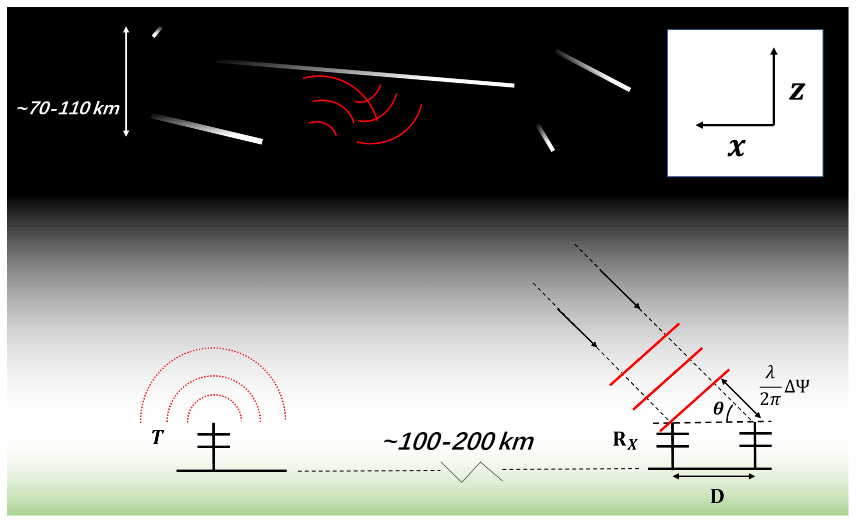
Figure 1 Schematic diagram of the simplified bistatic configuration used in Hocking's vertical resolution analysis (Hocking, 2018). The two receiving antennas and the transmitting antenna are collinear. The analysis is in a two-dimensional vertical section through the baseline joining the antennas. The radio wave is scattered from a few Fresnel zones that are several kilometers in length around the specular point on the meteor trail and are received by the receiving antennas. The cross-correlation analysis between the receiving antennas can be used to solve for the AoAs. Because the radio wave is reflected from a region a few Fresnel zones in length, the measured phase difference between the receiver antenna pairs to deviates from the ideal phase difference. This deviation from the ideal phase difference is one of the error sources in the PDME. In this work, we solve for the ideal phase difference associated with the AoA directed to the MTSP.

A number of recent studies have discussed AoA measurement errors for meteor radars (Kang, 2008; Vaudrin et al., 2018; Younger and Reid, 2017). These studies focus on the phase errors in receiver antenna pairs; see Younger and Reid (2017) for the monostatic case and Vaudrin et al. (2018) for a more general case that included multistatic meteor radars. Hocking (2018) used another approach and developed a vertical resolution analysis method for the two-dimensional bistatic case. The Hocking method (HM hereinafter) simplifies the error propagation process in the receiving antennas and puts emphasis on how a bistatic meteor radar configuration affects the vertical resolution in a vertical section. It does not consider the radial distance measuring error. In this paper, we consider the more general three-dimensional case and determine the spatial distribution of both the horizontal and vertical resolution uncertainties.

We analyze the multistatic meteor radar resolution distribution in a three-dimensional space for both vertical and horizontal resolution for the first time. This spatial resolution is a prerequisite for evaluating the reliability of retrieved atmospheric parameters, such as the wind field and the temperature.

2 Analytical method

2.1 Brief introduction

The HM will be introduced briefly here to help the reader understand our generalization. In the HM, measurement errors that affect the vertical resolution can be classified into two types: one caused by the zenith angle measuring error δθ and one caused by the pulse length effect on the vertical resolution. The receiving array is a simple antenna pair that is collinear with the baseline (Fig. 1). The HM calculates the vertical resolution in a two-dimensional vertical section that passes through the baseline. The receiver antenna pair is equivalent to one receiver arm in a Jones configuration that is comprised of three collinear antennas usually with a 2λ\2.5λ spacing. The phase difference of the received radio wave between the receiving antenna pair is denoted as ΔΨ. In meteor radar systems, there is generally an “acceptable” phase difference measuring error (PDME hereinafter) δ(ΔΨ). A higher value of δ(ΔΨ) means that more detected signals will be judged as meteor events but with more misidentifications and bigger errors as well. δ(ΔΨ) is set to approximately 30^∘ (Hocking, 2018; Younger and Reid, 2017) in most meteor radar systems. In the HM, the zenith angle measuring error δθ is due to δ(ΔΨ) and δ(ΔΨ) is a constant. Therefore, the error propagation in the receiver is very simple, and δθ is inversely proportional to the cosine of the zenith angle.

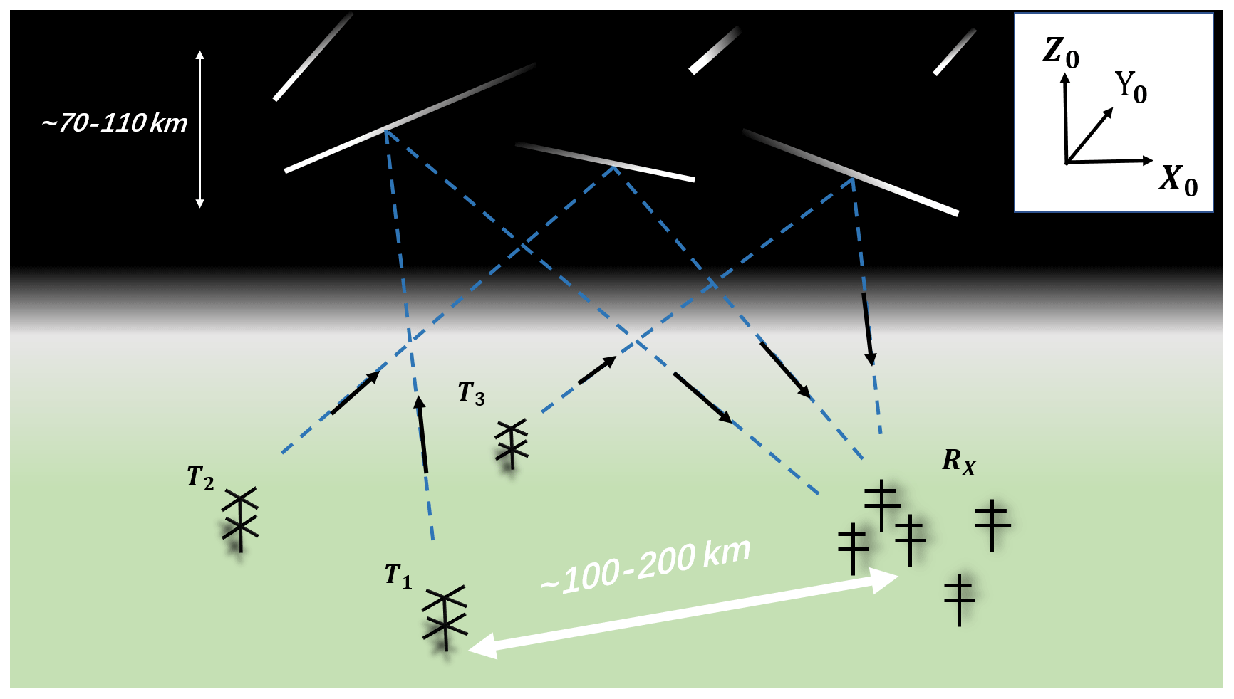
Figure 2 Schematic diagram of a multistatic meteor radar system using SIMO (single-input and multi-output). There are three transmitters (T₁, T₂ and T₃) and one receiver (R_X) in the picture. The transmitter–receiver distance is typically 100–200 km. X₀, Y₀ and Z₀ represent the east, north and up directions of the receiving antenna. Over 90 % of the received energy comes from about 1 km around the specular point of the meteor trail, which is slightly less than the length of the central Fresnel zone (Ceplecha et al., 1998).

We now introduce our analytical method. Our method considers a multistatic system with multiple transmitters and one receiving array in three-dimensional space as shown in Fig. 2. The receiving array is in the Jones configuration, that is, “cross-shaped”, but it may also be “T-shaped” or “L-shaped”. The five receiver antennas are in the same horizontal plane and constitute two orthogonal antenna arms. To avoid a complex error propagation process in the receiving array and to place emphasis on multistatic configurations, the PDMEs in the two orthogonal antenna arms (δ(ΔΨ₁) and δ(ΔΨ₂)) are constants. Therefore, the AoA measuring errors (including the zenith and azimuth angle measuring errors δθ, δϕ, respectively) can be expressed as simple functions of zenith and azimuth angle. The radial distance is the distance between the MTSP and the receiver, which is denoted as R_s. R_s can be determined by combining the AoA, baseline length d_i and the radio wave propagation path length R (Stober and Chau, 2015). The geometry is shown in Fig. 4a. α is the angle between the baseline (i.e.,X_i axis) and the line from the receiver to the MTSP (denoted as point A). If α, d_i and R are known, R_s can be calculated easily using the cosine law as follows:

$$\begin{array}{}\text{(1)}& R_{\mathrm{s}}={\displaystyle \frac{R^{\mathrm{2}}-d_i^{\mathrm{2}}}{\mathrm{2}(R-d_i\cos \mathit{\alpha })}}.\end{array}$$

A multistatic configuration will influence the accuracy of R_s (denoted as δR_s). This is because α, d and R are determined by the multistatic configuration. We consider the error term δR_s in our method, which is ignored in the HM. δR_s is a function of the AoA measuring errors (δθ and δϕ) and the radio wave propagation path length measuring error (denoted as δR). δR is caused by the measuring error of the wave propagation time δt, which is approximately 21 µs (Kang, 2008). Thus, δR can be set as a constant and the default value in our program is $\mathit{\delta }R=c\mathit{\delta }t=\mathrm{6.3}\mathrm{km}$. It is worth noting that the maximum unambiguous range for pulse meteor radars is determined by the pulse repetition frequency (PRF) (Hocking et al., 2001; Holdsworth et al., 2004). For multistatic meteor radars utilizing forward scatter, the maximum unambiguous range is $c/\text{PRF}$ (where c is the speed of light). For the area where R exceeds the maximum unambiguous range, δR is set to positive infinity.

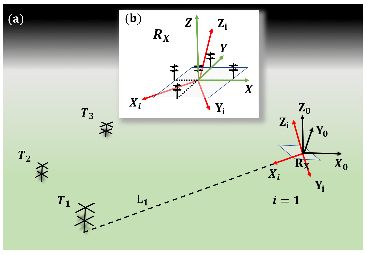
Figure 3 (a) Schematic diagram of the three coordinate systems used in this work. X_iY_iZ_i is a class of coordinate systems whose X_i axis points to transmitter i, with $i=\mathrm{1},\mathrm{2},\mathrm{3}$. X₀Y₀Z₀ is the ENU coordinate system to which all errors are compared. (b) Magnified plot of the receiving array. XYZ is fixed on the receiver horizontal plane. The x and y axes are collinear with the two arms of the antenna array.

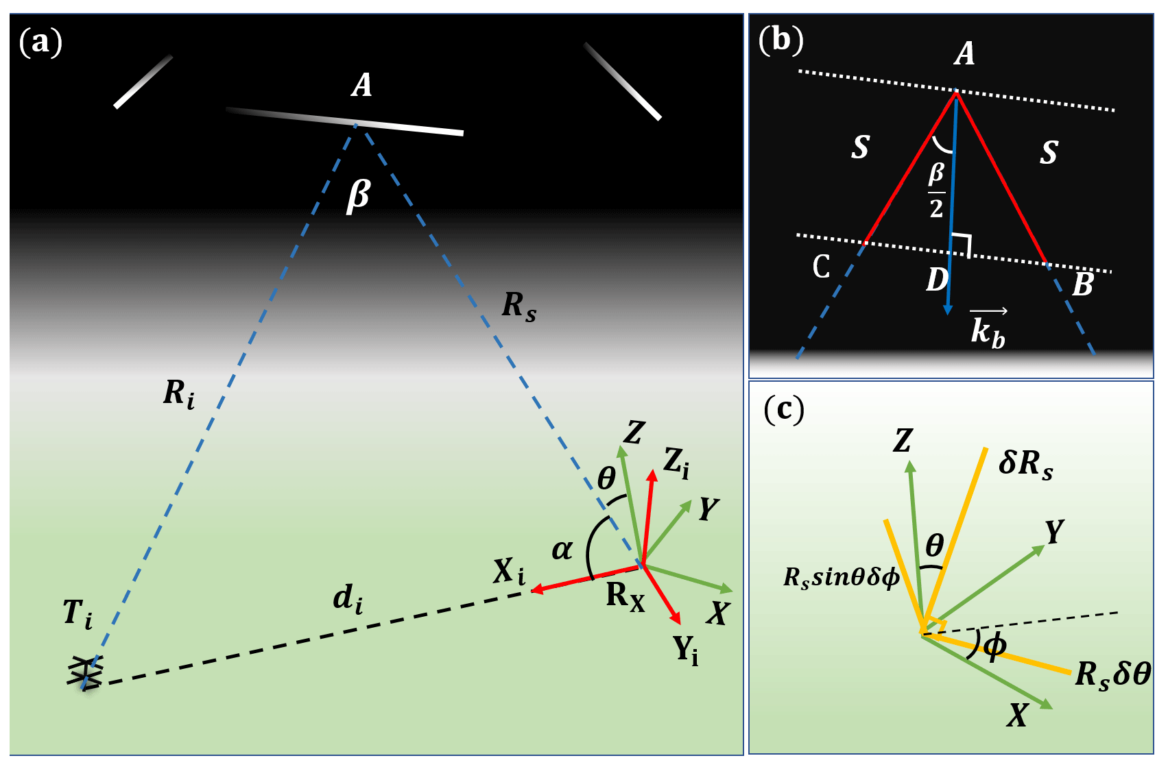
Figure 4 (a) Schematic diagram of the forward-scatter geometry for the radar link between T_i and R_X. Point A is the MTSP. (b) Magnified plot of specular point A. The red line represents a radio wave pulse, and S is the half-pulse length. k_b is the Bragg vector, which halves the forward-scatter angle β. (c) Schematic diagram of E₁ in XYZ, which can be decomposed into three orthogonal vectors.

2.2 Three kinds of coordinate systems and their transformations

To better depict the multistatic system configuration, three kinds of right-hand coordinate systems need to be established, as shown in Fig. 3. These are X₀Y₀Z₀, X_iY_iZ_i and XYZ. X₀Y₀Z₀ is the ENU (east–north–up) coordinate system where the X₀, Y₀ and Z₀ axes represent the east, north and up directions, respectively. Another two coordinate systems are established to facilitate different error propagations. All types of errors need to be transformed to the ENU coordinate system X₀Y₀Z₀ in the end. Coordinate system XYZ is established to depict the spatial configuration of the receiving array and has its the origin of XYZ there, as shown in Fig. 3. The z axis is collinear with the antenna boresight and perpendicular to the horizontal plane on which the receiving array lies. The x and y axes are collinear with the arms of the two orthogonal antenna arrays. AoAs will be represented in XYZ for convenience. Inspection of Fig. 4 indicates that it is convenient to analyze the range information in a plane that goes through the baseline and the MTSP. Thus, a coordinate system X_iY_iZ_i is established for a transmitter T_i. The coordinate origins of X_iY_iZ_i are all on the receiving array. We stipulate that the X_i axis points to transmitter i (T_i). Each pair T_i and receiver R_X constitute a radar link, which is referred to as L_i. The range-related information for each L_i will be calculated in X_iY_iZ_i. Different types of errors need to propagate to and be compared in X₀Y₀Z₀, which is convenient for retrieving wind fields.

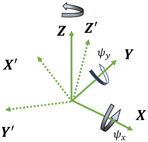
We stipulate that clockwise rotation satisfies the right-hand corkscrew rule. By rotating ${\mathit{\psi }}_x^{X,i}$, ${\mathit{\psi }}_y^{Y,i}$ and ${\mathit{\psi }}_z^{Z,i}$ about the x, y and z axes, respectively, one can transform XYZ to X_iY_iZ_i. It is worth mentioning that X_iY_iZ_i is non-unique because any rotation about X_i axis can obtain another satisfactory X_iY_iZ_i. Hence, ${\mathit{\psi }}_x^{X,i}$ can be set to any value. Similarly, by rotating ${\mathit{\psi }}_x^{\mathrm{i},\mathrm{0}}$, ${\mathit{\psi }}_y^{i,\mathrm{0}}$ and ${\mathit{\psi }}_z^{i,\mathrm{0}}$ about the x, y and z axes, respectively, one can transform X_iY_iZ_i to X₀Y₀Z₀. To realize the coordinate transformation between these three coordinate systems, a coordinate rotation matrix ${\mathbf{A}}_{\mathbf{R}}({\mathit{\psi }}_x,{\mathit{\psi }}_y,{\mathit{\psi }}_z)$ is introduced. Using A_R, one can transform the coordinate point or vector presentation from one coordinate system to another. The details of the coordinate rotation matrix ${\mathbf{A}}_{\mathbf{R}}({\mathit{\psi }}_x,{\mathit{\psi }}_y,{\mathit{\psi }}_z)$ can be found in Appendix A.

2.3 Two types of measuring errors

The analytical method of the spatial resolution for each radar link is the same. The difference between these radar links is only the value of the six coordinate rotation angles (${\mathit{\psi }}_x^{X,i}$, ${\mathit{\psi }}_y^{Y,i}$ and ${\mathit{\psi }}_z^{Z,i};{\mathit{\psi }}_x^{i,\mathrm{0}}$, ${\mathit{\psi }}_y^{i,\mathrm{0}}$ and ${\mathit{\psi }}_z^{i,\mathrm{0}}$) and the baseline distance d_i. The spatial-resolution-related measurement errors that will cause location errors of the MTSP can be classified into two types: E₁ is caused by measurement errors at the receiver, and E₂ is due to the pulse length. These two errors are mutually independent. Hence, the total error (E_total) can be expressed as follows:

$$\begin{array}{}\text{(2)}& E_{\text{total}}^{\mathrm{2}}=E_{\mathrm{1}}^{\mathrm{2}}+E_{\mathrm{2}}^{\mathrm{2}}.\end{array}$$

E₁ is related to three indirect measuring errors. They are zenith, azimuth and radial distance measuring errors, denoted as δθ, δϕ and δR_s, respectively. In XYZ, E₁ can be decomposed into three orthogonal error vectors using δθ, δϕ and δR_s (see Fig. 4c), which we now explain in more detail. PDMEs, i.e., δ(ΔΨ₁) and δ(ΔΨ₂), are caused by some practical factors, such as phase calibration mismatch and the fact that the specular point is not actually a point but is a few Fresnel zones in length. A meteor radar system calculates phase differences between different pairs of antenna through cross-correlation and then fits them to get the most likely AoAs. Therefore, the system needs to be assigned a tolerance value of δ(ΔΨ₁) and δ(ΔΨ₂). Different meteor radar systems have different AoA fit algorithms and thus different AoA measuring error distributions. To analyze the spatial resolution for a SIMO meteor radar system as generally as possible and to avoid tedious error propagation at the receiving array, we start the error propagation from δ(ΔΨ₁) and δ(ΔΨ₂) and set them as constants. AoA measuring errors δθ and δϕ can then be expressed as follows:

$$\begin{array}{}\text{(3)}& {\displaystyle }& {\displaystyle }\mathit{\delta }\mathit{\theta }={\displaystyle \frac{\mathit{\lambda }}{\mathrm{2}\mathit{\pi }{D}_{\mathrm{1}}}}{\displaystyle \frac{\cos \mathit{\varphi }}{\cos \mathit{\theta }}}\mathit{\delta }\left(\mathrm{\Delta }{\mathrm{\Psi }}_{\mathrm{1}}\right)+{\displaystyle \frac{\mathit{\lambda }}{\mathrm{2}\mathit{\pi }{D}_{\mathrm{2}}}}{\displaystyle \frac{\sin \mathit{\varphi }}{\cos \mathit{\theta }}}\mathit{\delta }\left(\mathrm{\Delta }{\mathrm{\Psi }}_{\mathrm{2}}\right),\text{(4)}& {\displaystyle }& {\displaystyle }\mathit{\delta }\mathit{\varphi }={\displaystyle \frac{\mathit{\lambda }}{\mathrm{2}\mathit{\pi }{D}_{\mathrm{2}}}}{\displaystyle \frac{\cos \mathit{\varphi }}{\sin \mathit{\theta }}}\mathit{\delta }\left(\mathrm{\Delta }{\mathrm{\Psi }}_{\mathrm{2}}\right)-{\displaystyle \frac{\mathit{\lambda }}{\mathrm{2}\mathit{\pi }{D}_{\mathrm{1}}}}{\displaystyle \frac{\sin \mathit{\varphi }}{\sin \mathit{\theta }}}\mathit{\delta }\left(\mathrm{\Delta }{\mathrm{\Psi }}_{\mathrm{1}}\right),\end{array}$$

where λ is the radio wavelength, D₁ and D₂ are the length of the two orthogonal antenna arms, and θ and ϕ are the zenith angle and the azimuth angle, respectively. The details can be found in Appendix A. It is worth noting that δθ and δϕ are not mutually independent. The expectation value of their product is not identical to zero unless $\frac{E\left({\mathit{\delta }}^{\mathrm{2}}\left(\mathrm{\Delta }{\mathrm{\Psi }}_{\mathrm{1}}\right)\right)}{D_{\mathrm{1}}^{\mathrm{2}}}$ is equal to $\frac{E\left({\mathit{\delta }}^{\mathrm{2}}\left(\mathrm{\Delta }{\mathrm{\Psi }}_{\mathrm{2}}\right)\right)}{D_{\mathrm{2}}^{\mathrm{2}}}$. δR_s can be expressed as a function of δR, δθ and δϕ as follows:

$$\begin{array}{}\text{(5)}& \begin{array}{rl}\mathit{\delta }{R}_{\mathrm{s}}& =F(\mathit{\delta }R,\mathit{\delta }\mathit{\theta },\mathit{\delta }\mathit{\varphi })\\ & =f_R(\mathit{\theta },\mathit{\varphi })\mathit{\delta }R+f_{\mathit{\theta }}(\mathit{\theta },\mathit{\varphi })\mathit{\delta }\mathit{\theta }+f_{\mathit{\varphi }}(\mathit{\theta },\mathit{\varphi })\mathit{\delta }\mathit{\varphi }.\end{array}\end{array}$$

$f_R(\mathit{\theta },\mathit{\varphi }),f_{\mathit{\theta }}(\mathit{\theta },\mathit{\varphi })$ and f_ϕ(θ,ϕ) are the weighting functions of δR_s. The details about the weighting function and deduction can be found in Appendix A. Inspection of Fig. 4c indicates that E₁ can be decomposed into three orthogonal error vectors in coordinate XYZ, denoted as δR_s, R_sδθ and R_ssin θδϕ. These three vectors can be expressed in XYZ as follows:

$$\begin{array}{}\text{(6)}& {\displaystyle }& {\displaystyle }\mathit{\delta }{\mathit{R}}_{\mathbf{s}}=\mathit{\delta }{R}_{\mathrm{s}}(\sin \mathit{\theta }\cos \mathit{\varphi },\sin \mathit{\theta }\sin \mathit{\varphi },\cos \mathit{\theta }{)}^{\mathrm{T}},\text{(7)}& {\displaystyle }& {\displaystyle }{\mathit{R}}_{\mathbf{s}}\mathit{\delta }\mathit{\theta }=R_{\mathrm{s}}\mathit{\delta }\mathit{\theta }(\cos \mathit{\theta }\cos \mathit{\varphi },\cos \mathit{\theta }\sin \mathit{\varphi },-\sin \mathit{\theta }{)}^{\mathrm{T}},\text{(8)}& {\displaystyle }& {\displaystyle }{\mathit{R}}_{\mathbf{s}}\mathbf{sin}\mathit{\theta }\mathit{\delta }\mathit{\varphi }=R_{\mathrm{s}}\sin \mathit{\theta }\mathit{\delta }\mathit{\varphi }(-\sin \mathit{\varphi },\cos \mathit{\varphi },\mathrm{0}{)}^{\mathrm{T}}.\end{array}$$

E₂ is related to the radio wave propagation path. A pulse might be reflected anywhere within a pulse length (see Fig. 4b). This causes a location error in the MTSP, represented as an error vector DA. D is the median point of the isosceles triangle ΔABC's side BC. The representation of the error vector DA can be solved in X_iY_iZ_i by using geometrical relationships as follows:

$$\begin{array}{}\text{(9)}& \begin{array}{rl}\mathit{D}\mathit{A}=(& {\displaystyle \frac{(\mathrm{2}-a_{\mathrm{1}}-a_{\mathrm{2}})x_i+d_i(a_{\mathrm{2}}-\mathrm{1})}{\mathrm{2}}},{\displaystyle \frac{(\mathrm{2}-a_{\mathrm{1}}-a_{\mathrm{2}})y_i}{\mathrm{2}}},\\ & {\displaystyle \frac{(\mathrm{2}-a_{\mathrm{1}}-a_{\mathrm{2}})z_i}{\mathrm{2}}}{)}^{\mathrm{T}},\end{array}\end{array}$$

where S is the half-pulse length and $a_{\mathrm{1}}=\frac{R_{\mathrm{s}}-S}{R_{\mathrm{s}}}$. $a_{\mathrm{2}}=\frac{R_i-S}{R_i}$. d_i is the baseline length. $(x_i,y_i,z_i)$ is the coordinate value of a MTSP (point A in Fig. 4) in X_iY_iZ_i. More details can be found in Appendix A.

2.4 Transformation to ENU coordinates

Thus far, two types of errors in different coordinate systems have been introduced. Now they need to be transformed to ENU coordinates X₀Y₀Z₀ in order to compare different radar links and to analyze the wind fields. E₁-related error vectors, which are three orthogonal vectors δR_s, R_sδθ, and R_ssin θδϕ, are represented in XYZ as Eqs. (6)–(8) and need to be transformed from XYZ to X₀Y₀Z₀ to project δR_s, R_sδθ and R_ssin θδϕ towards the X₀Y₀Z₀ axis, respectively, and reassemble them to form three new error vectors in the X₀Y₀Z₀ axis. Using the coordinate rotation matrix ${{\mathbf{A}}_{\mathbf{R}}}^{(XYZ,X_{\mathrm{0}}{Y}_{\mathrm{0}}{Z}_{\mathrm{0}})}={\mathbf{A}}_{\mathbf{R}}({\mathit{\psi }}_x^{i,\mathrm{0}},{\mathit{\psi }}_y^{i,\mathrm{0}},{\mathit{\psi }}_z^{i,\mathrm{0}})\cdot {\mathbf{A}}_{\mathbf{R}}({\mathit{\psi }}_x^{X,i},{\mathit{\psi }}_y^{Y,i},{\mathit{\psi }}_z^{Z,i})$ and Eqs. (6)–(8), the unit vectors of those three vectors can be represented in X₀Y₀Z₀ as follows:

$$\begin{array}{}\text{(10)}& \begin{array}{rl}& \left(\begin{array}{ccc}{\mathrm{X}}_{\mathrm{0}}^{\prime }\left(\mathit{\delta }{R}_{\mathrm{s}}\right)& {\mathrm{X}}_{\mathrm{0}}^{\prime }\left(\mathit{\delta }\mathit{\theta }\right)& {\mathrm{X}}_{\mathrm{0}}^{\prime }\left(\mathit{\delta }\mathit{\varphi }\right)\\ {\mathrm{Y}}_{\mathrm{0}}^{\prime }\left(\mathit{\delta }{R}_{\mathrm{s}}\right)& {\mathrm{Y}}_{\mathrm{0}}^{\prime }\left(\mathit{\delta }\mathit{\theta }\right)& {\mathrm{Y}}_{\mathrm{0}}^{\prime }\left(\mathit{\delta }\mathit{\varphi }\right)\\ {\mathrm{Z}}_{\mathrm{0}}^{\prime }\left(\mathit{\delta }{R}_{\mathrm{s}}\right)& {\mathrm{Z}}_{\mathrm{0}}^{\prime }\left(\mathit{\delta }\mathit{\theta }\right)& {\mathrm{Z}}_{\mathrm{0}}^{\prime }\left(\mathit{\delta }\mathit{\varphi }\right)\end{array}\right)={{\mathbf{A}}_{\mathbf{R}}}^{(XYZ,X_{\mathrm{0}}{Y}_{\mathrm{0}}{Z}_{\mathrm{0}})}\\ & \cdot \left(\begin{array}{ccc}\sin \mathit{\theta }\cos \mathit{\varphi }& \cos \mathit{\theta }\cos \mathit{\varphi }& -\sin \mathit{\varphi }\\ \sin \mathit{\theta }\sin \mathit{\varphi }& \cos \mathit{\theta }\sin \mathit{\varphi }& \cos \mathit{\varphi }\\ \cos \mathit{\theta }& -\sin \mathit{\theta }& \mathrm{0}\end{array}\right).\end{array}\end{array}$$

${\left({\mathbf{X}}_{\mathbf{0}}^{\mathbf{\prime }}\mathbf{\left(}\mathit{\delta }{\mathit{R}}_{\mathbf{s}}\mathbf{\right)}\mathbf{,}{\mathit{Y}}_{\mathbf{0}}^{\mathbf{\prime }}\mathbf{\left(}\mathit{\delta }{\mathit{R}}_{\mathbf{s}}\mathbf{\right)}\mathbf{,}{\mathit{Z}}_{\mathbf{0}}^{\mathbf{\prime }}\mathbf{\left(}\mathit{\delta }{\mathit{R}}_{\mathbf{s}}\mathbf{\right)}\right)}^{\mathbf{T}}$, ${\left({\mathit{X}}_{\mathbf{0}}^{\mathbf{\prime }}\mathbf{\left(}\mathit{\delta }\mathit{\theta }\mathbf{\right)}\mathbf{,}{\mathit{Y}}_{\mathbf{0}}^{\mathbf{\prime }}\mathbf{\left(}\mathit{\delta }\mathit{\theta }\mathbf{\right)}\mathbf{,}{\mathit{Z}}_{\mathbf{0}}^{\mathbf{\prime }}\mathbf{\left(}\mathit{\delta }\mathit{\theta }\mathbf{\right)}\right)}^{\mathbf{T}}$, and ${\left({\mathit{X}}_{\mathbf{0}}^{\mathbf{\prime }}\mathbf{\left(}\mathit{\delta }\mathit{\varphi }\mathbf{\right)}\mathbf{,}{\mathit{Y}}_{\mathbf{0}}^{\mathbf{\prime }}\mathbf{\left(}\mathit{\delta }\mathit{\varphi }\mathbf{\right)}\mathbf{,}{\mathit{Z}}_{\mathbf{0}}^{\mathbf{\prime }}\mathbf{\left(}\mathit{\delta }\mathit{\varphi }\mathbf{\right)}\right)}^{\mathbf{T}}$ are unit vectors of δR_s, R_sδθ, and R_ssin θδϕ in X₀Y₀Z₀, respectively. The 3×3 matrix on the left-hand side of Eq. (10) is denoted as P_ij for $i,j=\mathrm{1},\mathrm{2},\mathrm{3}$.

From Eqs. (6)–(8) and Fig. 4c, we see that the length of those three vectors (the error values) is δR_s, R_sδθ, R_ssin θδϕ as a function of δR, δθ, δϕ. In order to reassemble them to form new error vectors, transformation of δθ and δϕ into two independent errors δ(ΔΨ₁) and δ(ΔΨ₂) is needed because δθ and δϕ are not independent. Using Eqs. (3) and (4), one can transform vector ${\left(\mathit{\delta }R,\mathit{\delta }\mathit{\theta },\mathit{\delta }\mathit{\varphi }\right)}^{\mathrm{T}}$ into three independent measuring errors δR, δ(ΔΨ₁) and δ(ΔΨ₂). Thus, ${\left(\mathit{\delta }{R}_{\mathrm{s}},R_{\mathrm{s}}\mathit{\delta }\mathit{\theta },R_{\mathrm{s}}\sin \mathit{\theta }\mathit{\delta }\mathit{\varphi }\right)}^{\mathrm{T}}$ can be expressed as follows:

$$\begin{array}{}\text{(11)}& \begin{array}{rl}\left(\begin{array}{c}\mathit{\delta }{R}_{\mathrm{s}}\\ R_{\mathrm{s}}\mathit{\delta }\mathit{\theta }\\ R_{\mathrm{s}}\sin \mathit{\theta }\mathit{\delta }\mathit{\varphi }\end{array}\right)& =\left(\begin{array}{ccc}{f}_R(\mathit{\theta },\mathit{\varphi })& f_{\mathit{\theta }}(\mathit{\theta },\mathit{\varphi })& f_{\mathit{\varphi }}(\mathit{\theta },\mathit{\varphi })\\ \mathrm{0}& R_{\mathrm{s}}& \mathrm{0}\\ \mathrm{0}& \mathrm{0}& R_{\mathrm{s}}\sin \mathit{\theta }\end{array}\right)\\ & \cdot \left(\begin{array}{ccc}\mathrm{1}& \mathrm{0}& \mathrm{0}\\ \mathrm{0}& \frac{\frac{\mathit{\lambda }}{\mathrm{2}\mathit{\pi }}}{\cos \mathit{\theta }}\frac{\cos \mathit{\varphi }}{D_{\mathrm{1}}}& -\frac{\frac{\mathit{\lambda }}{\mathrm{2}\mathit{\pi }}\sin \mathit{\varphi }}{\sin \mathit{\theta }{D}_{\mathrm{1}}}\\ \mathrm{0}& \frac{\frac{\mathit{\lambda }}{\mathrm{2}\mathit{\pi }}}{\cos \mathit{\theta }}\frac{\sin \mathit{\varphi }}{D_{\mathrm{2}}}& \frac{\frac{\mathit{\lambda }}{\mathrm{2}\mathit{\pi }}\cos \mathit{\varphi }}{\sin \mathit{\theta }{D}_{\mathrm{2}}}\end{array}\right)\\ & \cdot \left(\begin{array}{c}\mathit{\delta }R\\ \mathit{\delta }\left(\mathrm{\Delta }{\mathrm{\Psi }}_{\mathrm{1}}\right)\\ \mathit{\delta }\left(\mathrm{\Delta }{\mathrm{\Psi }}_{\mathrm{2}}\right)\end{array}\right).\end{array}\end{array}$$

The product of the first and the second term on the right-hand side of Eq. (11) is a 3×3 matrix, denoted as W_ij for $i,j=\mathrm{1},\mathrm{2},\mathrm{3}$. From Eq. (11), we see that the three error values δR_s, R_sδθ and R_ssin θδϕ are the linear combinations of δR, δ(ΔΨ₁),and δ(ΔΨ₂) with their corresponding linear coefficients W_1j, W_2j and W_3j. Those three error values can be projected toward new directions (e.g., the X₀Y₀Z₀ axis) by using P_ij. It worth noting that in a new direction the same basis's projected linear coefficients from different error values should be used to calculate their sum of squares (SS). Following this, the square root of SS will be used as a new linear coefficient for that basis in the new direction. For example, in X₀ directions, basis δ(ΔΨ₁)'s projected linear coefficients are ${\mathrm{X}}_{\mathrm{0}}^{\prime }\left(\mathit{\delta }{R}_{\mathrm{s}}\right)W_{\mathrm{12}}$, ${\mathrm{X}}_{\mathrm{0}}^{\prime }\left(\mathit{\delta }\mathit{\theta }\right)W_{\mathrm{22}}$ and ${\mathrm{X}}_{\mathrm{0}}^{\prime }\left(\mathit{\delta }\mathit{\varphi }\right)W_{\mathrm{32}}$ from δR_s, R_sδθ and R_ssin θδϕ, respectively. Therefore, the new linear coefficient for δ(ΔΨ₁) in the X₀ direction is $W_{{\mathrm{X}}_{\mathrm{0}}^{\prime }}^{\mathit{\delta }\left(\mathrm{\Delta }{\mathrm{\Psi }}_{\mathrm{1}}\right)}=\pm \sqrt{{\left({\mathrm{X}}_{\mathrm{0}}^{\prime }\left(\mathit{\delta }{R}_{\mathrm{s}}\right)W_{\mathrm{12}}\right)}^{\mathrm{2}}+{\left({\mathrm{X}}_{\mathrm{0}}^{\prime }\left(\mathit{\delta }\mathit{\theta }\right)W_{\mathrm{22}}\right)}^{\mathrm{2}}+{\left({\mathrm{X}}_{\mathrm{0}}^{\prime }\left(\mathit{\delta }\mathit{\varphi }\right)W_{\mathrm{32}}\right)}^{\mathrm{2}}}$. Similarly, one can get δR and δ(ΔΨ₂)'s new linear coefficients in ${\mathrm{X}}_{\mathrm{0}}^{\prime }$, denoted as $W_{{\mathrm{X}}_{\mathrm{0}}^{\prime }}^{\mathit{\delta }R}$ and $W_{{\mathrm{X}}_{\mathrm{0}}^{\prime }}^{\mathit{\delta }\left(\mathrm{\Delta }{\mathrm{\Psi }}_{\mathrm{2}}\right)}$. Thus, the true error value in the X₀ direction is $W_{{\mathrm{X}}_{\mathrm{0}}^{\prime }}^{\mathit{\delta }R}\mathit{\delta }R+W_{{\mathrm{X}}_{\mathrm{0}}^{\prime }}^{\mathit{\delta }\left(\mathrm{\Delta }{\mathrm{\Psi }}_{\mathrm{1}}\right)}\mathit{\delta }\left(\mathrm{\Delta }{\mathrm{\Psi }}_{\mathrm{1}}\right)+W_{{\mathrm{X}}_{\mathrm{0}}^{\prime }}^{\mathit{\delta }\left(\mathrm{\Delta }{\mathrm{\Psi }}_{\mathrm{2}}\right)}\mathit{\delta }\left(\mathrm{\Delta }{\mathrm{\Psi }}_{\mathrm{2}}\right)$. Because δR, δ(ΔΨ₁), and δ(ΔΨ₂) are mutually independent, E₁ is related to the mean squared error (MSE) values in the X₀ direction, denoted as δ₍₁₎X₀ and can be expressed as ${\mathit{\delta }}_{\left(\mathrm{1}\right)}{X}_{\mathrm{0}}=\pm$ $\sqrt{{\left(W_{X_{\mathrm{0}}^{\prime }}^{\mathit{\delta }R}\mathit{\delta }R\right)}^{\mathrm{2}}+{\left(W_{X_{\mathrm{0}}^{\prime }}^{\mathit{\delta }\left(\mathrm{\Delta }{\mathrm{\Psi }}_{\mathrm{1}}\right)}\mathit{\delta }\left(\mathrm{\Delta }{\mathrm{\Psi }}_{\mathrm{1}}\right)\right)}^{\mathrm{2}}+{\left(W_{X_{\mathrm{0}}^{\prime }}^{\mathit{\delta }\left(\mathrm{\Delta }{\mathrm{\Psi }}_{\mathrm{2}}\right)}\mathit{\delta }\left(\mathrm{\Delta }{\mathrm{\Psi }}_{\mathrm{2}}\right)\right)}^{\mathrm{2}}}$.

In short, E₁-related errors in ENU coordinate's three axis directions (denoted as δ₍₁₎X₀, δ₍₁₎Y₀ and δ₍₁₎Z₀) can be expressed in the form of a matrix as follows:

$$\begin{array}{}\text{(12)}& \left(\begin{array}{c}{\mathit{\delta }}_{\left(\mathrm{1}\right)}^{\mathrm{2}}{X}_{\mathrm{0}}\\ {\mathit{\delta }}_{\left(\mathrm{1}\right)}^{\mathrm{2}}{Y}_{\mathrm{0}}\\ {\mathit{\delta }}_{\left(\mathrm{1}\right)}^{\mathrm{2}}{Z}_{\mathrm{0}}\end{array}\right)=P_{ij}^{\mathrm{2}}\cdot W_{ij}^{\mathrm{2}}\cdot \left(\begin{array}{c}{\mathit{\delta }}^{\mathrm{2}}R\\ {\mathit{\delta }}^{\mathrm{2}}\left(\mathrm{\Delta }{\mathrm{\Psi }}_{\mathrm{1}}\right)\\ {\mathit{\delta }}^{\mathrm{2}}\left(\mathrm{\Delta }{\mathrm{\Psi }}_{\mathrm{2}}\right)\end{array}\right).\end{array}$$

The E₂-related error vector DA needs transformation from X_iY_iZ_i to X₀Y₀Z₀. Therefore, E₂-related errors in the ENU coordinate's three axis directions (denoted as δ₍₂₎X₀, δ₍₂₎Y₀ and δ₍₂₎Z₀) can be expressed in the form of a matrix as follows:

$$\begin{array}{}\text{(13)}& \left(\begin{array}{c}{\mathit{\delta }}_{\left(\mathrm{2}\right)}{X}_{\mathrm{0}}\\ {\mathit{\delta }}_{\left(\mathrm{2}\right)}{Y}_{\mathrm{0}}\\ {\mathit{\delta }}_{\left(\mathrm{2}\right)}{Z}_{\mathrm{0}}\end{array}\right)=\pm {\mathbf{A}}_{\mathbf{R}}({\mathit{\psi }}_x^{i,\mathrm{0}},{\mathit{\psi }}_y^{i,\mathrm{0}},{\mathit{\psi }}_z^{i,\mathrm{0}})\cdot \mathit{D}\mathit{A}.\end{array}$$

E₁ and E₂ are mutually independent. By using Eq. (1), the total MSE values in ENU coordinate's three axis directions (denoted as δ_totalX₀, δ_totalY₀ and δ_totalZ₀) can be expressed in the form of matrix as follows:

$$\begin{array}{}\text{(14)}& \left(\begin{array}{c}{\mathit{\delta }}_{\text{total}}^{\mathrm{2}}{X}_{\mathrm{0}}\\ {\mathit{\delta }}_{\text{total}}^{\mathrm{2}}{Y}_{\mathrm{0}}\\ {\mathit{\delta }}_{\text{total}}^{\mathrm{2}}{Z}_{\mathrm{0}}\end{array}\right)=\left(\begin{array}{c}{\mathit{\delta }}_{\left(\mathrm{1}\right)}^{\mathrm{2}}{X}_{\mathrm{0}}\\ {\mathit{\delta }}_{\left(\mathrm{1}\right)}^{\mathrm{2}}{Y}_{\mathrm{0}}\\ {\mathit{\delta }}_{\left(\mathrm{1}\right)}^{\mathrm{2}}{Z}_{\mathrm{0}}\end{array}\right)+\left(\begin{array}{c}{\mathit{\delta }}_{\left(\mathrm{2}\right)}^{\mathrm{2}}{X}_{\mathrm{0}}\\ {\mathit{\delta }}_{\left(\mathrm{2}\right)}^{\mathrm{2}}{Y}_{\mathrm{0}}\\ {\mathit{\delta }}_{\left(\mathrm{2}\right)}^{\mathrm{2}}{Z}_{\mathrm{0}}\end{array}\right).\end{array}$$

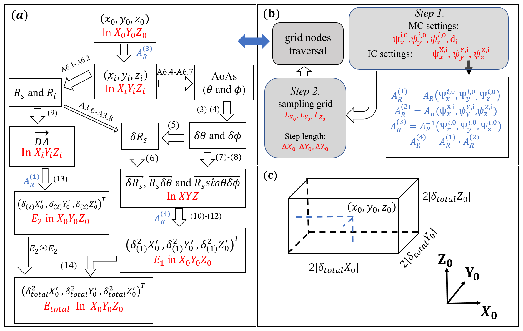
Figure 5 (a) The flow chart of the location error calculation process for a point in X₀Y₀Z₀. The notation beside the arrows represents the corresponding equations (black) or coordinate rotation matrix (blue) in the paper. ⊙ is the Hadamard product. Thus, E₂⊙E₂ will yield $({\mathit{\delta }}_{\left(\mathrm{2}\right)}^{\mathrm{2}}{X}_{\mathrm{0}},{\mathit{\delta }}_{\left(\mathrm{2}\right)}^{\mathrm{2}}{Y}_{\mathrm{0}},{\mathit{\delta }}_{\left(\mathrm{2}\right)}^{\mathrm{2}}{Z}_{\mathrm{0}}{)}^{\mathrm{T}}$. (b) The flow chart of the program to calculate the location errors distributions for a radar link L_i. This process includes parameters settings for a radar link, the generation of the sampling grid nodes and the traversing of all the nodes. For each node, the program uses the calculation method described in (a). MC is the multistatic configuration, and IC is the interferometer (receiving antenna) configuration. (c) Schematic diagram of the relationship between the spatial resolution and the total location errors of the MTSP. For a detected point in space, the MSE of MTSP's location errors is ±|δ_totalX₀|, ±|δ_totalY₀| and ±|δ_totalZ₀| in the zonal, meridional and vertical directions, respectively. This means that the actual specular point might occur in a region that forms a $\mathrm{2}\mathrm{|}{\mathit{\delta }}_{\text{total}}{X}_{\mathrm{0}}\mathrm{|}\times \mathrm{2}\mathrm{|}{\mathit{\delta }}_{\text{total}}{Y}_{\mathrm{0}}\mathrm{|}\times \mathrm{2}\mathrm{|}{\mathit{\delta }}_{\text{total}}{Z}_{\mathrm{0}}\mathrm{|}$ cube and that the detected point is on the centroid of this cube.

In conclusion, for a radar link L_i and a MTSP represented as $(x_{\mathrm{0}},y_{\mathrm{0}},z_{\mathrm{0}})$ in the ENU coordinate system X₀Y₀Z₀, as sketched in Fig. 4a, the location errors of this point in east, north and up directions (±δ_totalX₀, ±δ_totalY₀ and ±δ_totalZ₀) can be calculated as follows: firstly, for a point $(x_{\mathrm{0}},y_{\mathrm{0}},z_{\mathrm{0}})$ in ${\mathrm{X}}_{\mathrm{0}}^{\prime }{Y}_{\mathrm{0}}^{\prime }{\mathrm{Z}}_{\mathrm{0}}^{\prime }$, use A_R to transform it to X_iY_iZ_i and denote it as $(x_i,y_i,z_i)$. Following this, in X_iY_iZ_i calculate the AoA (θ and ϕ) and the range information (R_s and R_i). Details of AoA and range calculation can be found in Appendix A. It is worth noting that the AoA is given by the angles relative to the axes of XYZ. Secondly, in XYZ use the AoA and Eqs. (3)–(8) to calculate E₁'s three orthogonal error vectors shown in Fig. 4c; in X_iY_iZ_i use the range information and Eq. (9) to calculate E₂'s error vector DA, as shown in Fig. 4b. Thirdly, project E₁'s three error vectors to X₀Y₀Z₀ by using Eq. (10) and use Eqs. (11)–(12) to reassemble them to calculate E₁-related MSE values in the direction of X₀Y₀Z₀; use Eq. (13) to transform the E₂ error vector from X_iY_iZ_i to X₀Y₀Z₀. Finally, use Eq. (14) to get the total location errors of a MTSP in $(x_{\mathrm{0}},y_{\mathrm{0}},z_{\mathrm{0}})$. Figure 5a shows the flow chart for the process we have just described.

3 Results and discussion

The program to study the method we have described above is written in the Python language and is presented in the Supplement. To calculate a special configuration of a multistatic radar system, we initially need to set six coordinate transformation angles (${\mathit{\psi }}_x^{X,i}$, ${\mathit{\psi }}_y^{Y,i}$ and ${\mathit{\psi }}_z^{Z,i};{\mathit{\psi }}_x^{i,\mathrm{0}}$, ${\mathit{\psi }}_y^{i,\mathrm{0}}$ and ${\mathit{\psi }}_z^{i,\mathrm{0}}$) and the baseline length d_i for each radar link L_i. For example, ${\mathit{\psi }}_x^{i,\mathrm{0}}={\mathit{\psi }}_y^{i,\mathrm{0}}=\mathrm{0}$, ${\mathit{\psi }}_z^{i,\mathrm{0}}=\mathrm{30}{}^{\circ }$ and d_i=250 km means that transmitter T_i is 250 km, 30^∘ east by south of the receiver R_X. Further, ${\mathit{\psi }}_x^{X,i}=\mathrm{5}$^∘, ${\mathit{\psi }}_y^{Y,i}=\mathrm{0}$, ${\mathit{\psi }}_z^{Z,i}=\mathrm{0}$ means one receiver arm (y axis) points to 60^∘ east by north with a 5^∘ elevation. The detection area of interest for a multistatic meteor radar is usually from 70 to 110 km in height and around 300 km × 300 km in the horizontal. In our program, this area needs to be divided into a spatial grid for sampling. The default value of the sampling grid length is 1 km in height and 5 km in the meridional and zonal directions. After selecting the desired settings, the program steps though the sampling grid nodes and calculates the location errors at each node as described in Fig. 5a. Figure 5b describes the parameter settings and the transversal calculation process. For a given setting of radar link L_i, the program will output the squared values of E₁-related, E₂-related and total MSE values ($E_{\text{total}}^{\mathrm{2}}$: ${\mathit{\delta }}_{\text{total}}^{\mathrm{2}}{X}_{\mathrm{0}},{\mathit{\delta }}_{\text{total}}^{\mathrm{2}}{Y}_{\mathrm{0}},{\mathit{\delta }}_{\text{total}}^{\mathrm{2}}{Z}_{\mathrm{0}}$; $E_{\mathrm{1}}^{\mathrm{2}}$: ${\mathit{\delta }}_{\left(\mathrm{1}\right)}^{\mathrm{2}}{X}_{\mathrm{0}}$, ${\mathit{\delta }}_{\left(\mathrm{1}\right)}^{\mathrm{2}}{Y}_{\mathrm{0}},{\mathit{\delta }}_{\left(\mathrm{1}\right)}^{\mathrm{2}}{Z}_{\mathrm{0}}$; $E_{\mathrm{2}}^{\mathrm{2}}$: ${\mathit{\delta }}_{\left(\mathrm{2}\right)}^{\mathrm{2}}{X}_{\mathrm{0}},{\mathit{\delta }}_{\left(\mathrm{2}\right)}^{\mathrm{2}}{Y}_{\mathrm{0}},{\mathit{\delta }}_{\left(\mathrm{2}\right)}^{\mathrm{2}}{Z}_{\mathrm{0}}$). The location errors can be positive or negative, and thus the spatial resolutions are twice the absolute value of the location errors. For an example, see Fig. 5c. For a detected MTSP, represented as $(x_{\mathrm{0}},y_{\mathrm{0}},z_{\mathrm{0}})$ in X₀Y₀Z₀, with ${\mathit{\delta }}_{\text{total}}^{\mathrm{2}}{X}_{\mathrm{0}},{\mathit{\delta }}_{\text{total}}^{\mathrm{2}}{Y}_{\mathrm{0}}$ and ${\mathit{\delta }}_{\text{total}}^{\mathrm{2}}{Z}_{\mathrm{0}}$ equal to 25, 16 and 9 km², respectively, the actual position of the MTSP could occur in an area that is ± 5, ± 4 and ± 3 km around $(x_{\mathrm{0}},y_{\mathrm{0}},z_{\mathrm{0}})$ with equal probability. Consequently, the zonal, meridional and vertical resolutions are 10, 8 and 6 km, respectively.

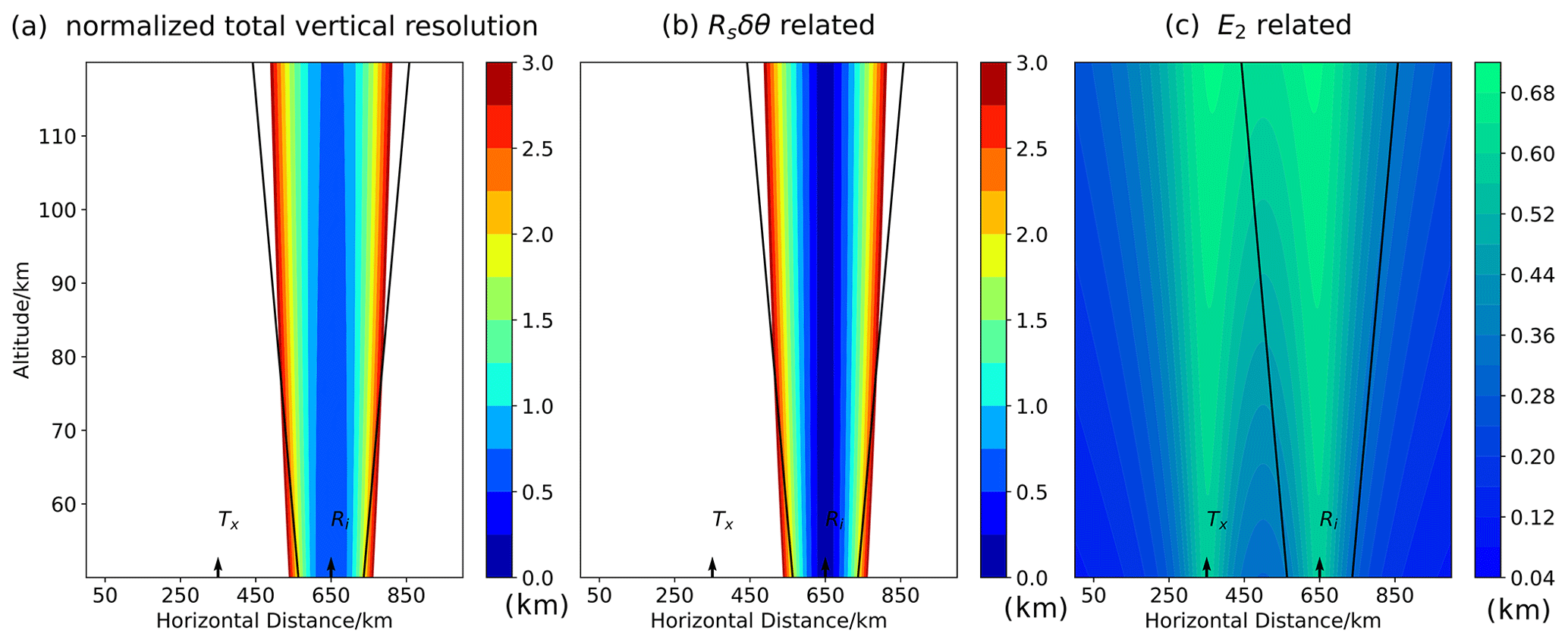
Figure 6 The normalized vertical resolution distribution in a vertical section from 50 to 120 km height when the error term “δR_s” is ignored. Panels (a–c) are the total, R_sδθ-related and E₂-related normalized resolution distributions, respectively. These results are the same as those produced in Hocking's work (Hocking, 2018). The two black arrows represent the positions right above the transmitter (Tx) and the receiver (Rx) and the transmitter–receiver separation is 300 km. The region between the two oblique black lines is the sampling volume for the receiving array because the elevation angle is beyond 30^∘ to reduce influence from potential mutual antenna coupling or from other obstacles in the surrounding area. Except the region at large elevation angles (i.e., 90^∘), the E₂-related resolution values are much lower than the R_sδθ-related errors. The R_sδθ-related resolution distribution only depends on the receiving antennas. Thus, the total vertical resolution distribution is nearly unchanged with the variation of the transmitter–receiver distance. Normalized resolution values that exceed 3 km (which correspond 12 km vertical resolution) are not shown.

The HM analyzes the vertical resolution (corresponding to δZ₀ in our paper) in a two-dimensional vertical section (corresponding to the X₀Z₀ plane in our paper). To compare with Hocking's work, ${\mathit{\psi }}_z^{i,\mathrm{0}}$ is set to 180^∘, and the other five coordinate transformation angles are all set to zero with d equal to 300 km. The half-pulse length S is set to 2 km and δ(ΔΨ₁) to 35^∘. Calculating in the X₀Y₀ plane only should have degraded our method into Hocking's two-dimensional analysis method but does not because the HM method ignores δR_s. In fact, the HM considers only E₂ and R_sδθ in the X₀Y₀ plane. Consequently, we need to further set f_R(θ,ϕ), f_θ(θ,ϕ) and f_ϕ(θ,ϕ) to be zero. When this is done, our method degrades into the HM. Hocking's results are shown as the absolute value of vertical location error normalized relative to the half-pulse width $\mathrm{|}\mathit{\delta }{Z}_{\mathrm{0}}\mathrm{|}/S$. Hereinafter, $\mathrm{|}E\mathrm{|}/S$ is referred to as the normalized spatial resolution, such as δ₍₁₎X₀ and δ_totalY₀, where E represents the location errors in a direction. Thus, the spatial resolutions are 2S times the normalized spatial resolutions.

Our normalized vertical resolution distributions are shown in Fig. 6a and are the same as those presented in Hocking's work (Hocking, 2018). The distribution of R_sδθ-related, E₂-related and total normalized vertical resolution distributions are shown in Fig. 6 from left to right, respectively. In most cases, E₂ is an order of magnitude smaller than R_sδθ. Only in the region directly above the receiver does E₂ have the same magnitude as R_sδθ. In other words, only in the region directly above the receiver can E₂ influence the total resolution. E₂ is related to the bistatic configuration but R_sδθ is not. Therefore, in the HM, the distribution of the total vertical resolution varies slightly with d. After adding the error term δR_t, which is related to the bistatic configuration, the normalized total vertical spatial-resolution distribution changes more obviously with d, as the first two rows in Fig. 7 show. The region between the two black lines represents the sampling volume for the receiver where the elevation angle is beyond 30^∘. As the transmitter–receiver distance becomes longer, resolutions in this sampling volume are not always acceptable. In the first row of Fig. 7, the transmitter–receiver distance is 300 km and about half of the region between the two black lines has normalized vertical resolution values larger than 3 km. Because our analytical method can obtain spatial resolutions in three-dimensional space, the third row of Fig. 7 shows the horizontal section at 90 km altitude for the second row of Fig. 7.

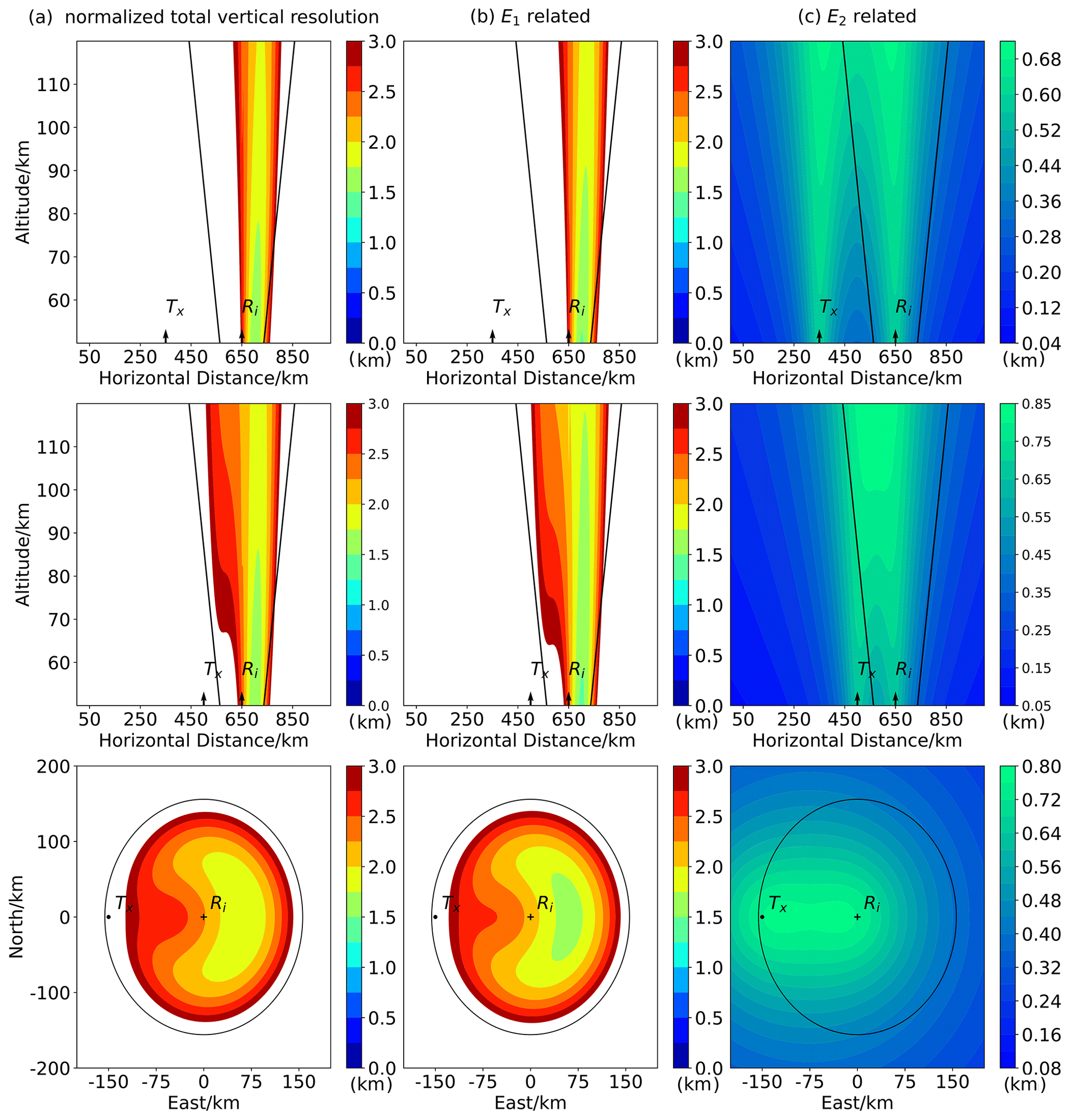
Figure 7 The normalized vertical resolution distribution using the analytical method described in this paper. The first and second rows represent a vertical section of height from 50 to 120 km. The third row represents the horizontal section at 90 km, and the receiving array is at the origin, with positive coordinate values representing the eastward or northward directions. The first row has the same parameters settings as Fig. 6 and is used to compare with Fig. 6. The E₁-related resolution will change with the transmitter–receiver configuration because it considers the error term “δR_s”. Thus, the total vertical resolution will change with the transmitter–receiver configuration. With the transmitter–receiver distance varying from 300 km (the first row) to 150 km (the second row), the total vertical resolution distribution is clearly changed. The third row is the perspective to the horizontal section at 90 km altitude for the second row. Normalized resolution values that exceed 3 km are not shown.

To get a perspective on the spatial-resolution distribution in three-dimensional space, Fig. 8 shows the normalized zonal, meridional and vertical spatial-resolution distributions for a multistatic radar link whose transmitter–receiver separation is 180 km and the transmitter is 30^∘ south by east of the receiver. The classic monostatic meteor radar is a special case of a multistatic meteor radar system whose the baseline length is zero. By setting the transmitter–receiver distance to be zero in our program, a monostatic meteor radar's spatial resolution can also be obtained. In this case, the spatial-resolution distributions are highly symmetrical and correspond to the real characteristics of monostatic meteor radar (this is not shown here but can be found in Fig. S1 in the Supplement). In the discussion above, the receiver and transmitter antennas are all coplanar. By varying ${\mathit{\psi }}_x^{X,i}$, ${\mathit{\psi }}_y^{Y,i}$ and ${\mathit{\psi }}_z^{Z,i}$ in our program, non-coplanar receiver–transmitter antenna situations can also be studied. Slightly tilting the receiver horizontal plane (for example, set ${\mathit{\psi }}_x^{X,i}={\mathit{\psi }}_y^{Y,i}=\mathrm{5}{}^{\circ }$) causes the horizontal spatial distributions to change (see Figs. S2 and S3 in the Supplement). In practice, the Earth's curvature and local topography will lead to tilts in the receiver horizontal plane. This kind of tilt should be taken into account for multistatic meteor radar systems, and details relating to the parameter selections for this can be found in the Supplement.

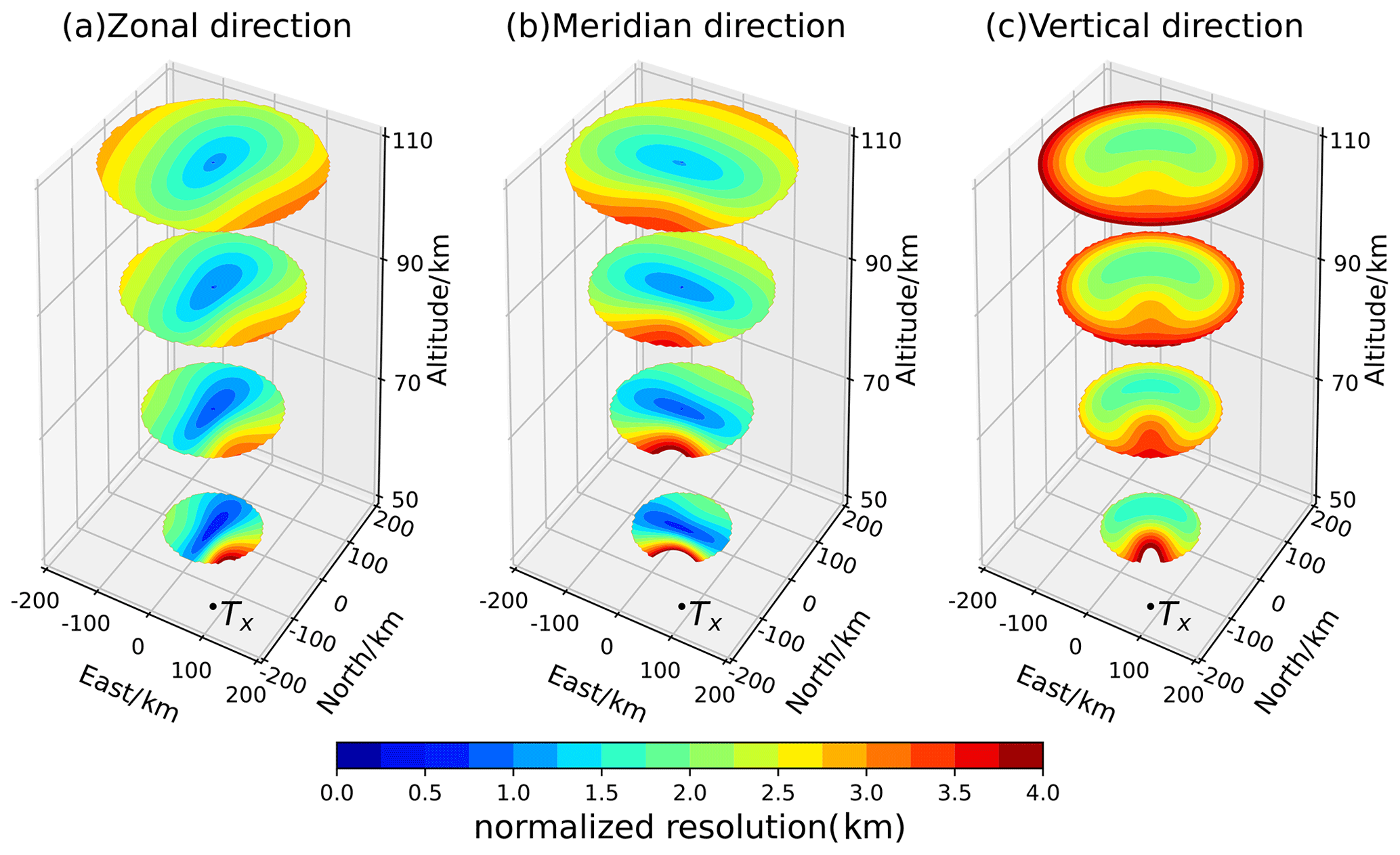
Figure 8 The 3D contour plot of the normalized resolution distribution for a multistatic radar link whose baseline length is 180 km and whose transmitter is 30^∘ south by east of the receiver. The black dots represent the position right above the transmitter, and the receiving array is at the origin of the axes. Panels (a–c) are the normalized resolution distributions in the zonal, meridional and vertical directions, respectively. The subplot's four slice circles from bottom to top are the horizontal section at 50, 70, 90 and 110 km height, respectively. The region whose elevation angle of the receiver is less than 30^∘ is not shown, and therefore the slice circles become larger from the bottom to the top. Normalized resolution values that exceed 4 km (which corresponds to 16 km resolution) are not shown.

The AoA error propagation process has been simplified to yield Eqs. (3) and (4) by using constant PDMEs. This is for the sake of providing the most general example of our method. If the analysis of AoA errors were to start from the original received voltage signals (e.g., Vaudrin et al., 2018), the error propagation process would depend on the specific receiver interferometer configuration and the specific signal processing method. The approach used here can be applied to different receiver antenna configurations or new signal processing algorithms. This would involve substitution of δ(ΔΨ₁) and δ(ΔΨ₂) into other mutually independent measuring errors to suit the experimental arrangement and then establishing a new AoA error propagation to obtain δθ and δϕ. This means rewriting the second and third term in Eq. (11) to the determine a new AoA error propagation matrix and new mutually independent measuring errors, respectively.

It worth noting that except for using the PDMEs as the start of the error propagation, all the analytical processes are built on mathematical error propagations. PDMEs include uncontrolled errors, such as those resulting from the returned wave being scattered from a few Fresnel zones along the meteor trail, phase calibration inaccuracy and noise. However, there are other error sources in practice. For example, aircraft or lightning interference and fading clutter from obstacles can cause further measurement errors in the AoA. These issues are related to actual physical situations and are beyond the scope of this text.

Knowing the valid observational volume for meteor detections and the errors associated with each detection is vital for a meteor radar system as it determines which meteors can be used to calculate wind velocities and also the uncertainties associated with the winds themselves. To reduce the influence of mutual antenna coupling or ground clutter, the elevation angle of a detection should be above a threshold, with 30^∘ being typically used, and this sets the basic valid observational volume. Within this, the normalized vertical resolution varies, and in Figs. 7 and S4 in the Supplement only the areas of normalized vertical resolution with values below 3 km are shown, which we argue represents an acceptable sampling volume. In addition, as the transmitter–receiver distance increases, the sampling volume becomes smaller and the vertical resolution in this volume is reduced. This effect limits the practically usable transmitter–receiver distances for multistatic meteor radars.

The geometry of the multistatic meteor radar case also impacts on the ability of the radar to measure the Doppler shifts associated with drifting meteor trails within the observational volume. This is because the measured Doppler shift is produced by the component of the wind field in the direction of the Bragg vector, which in the multistatic configuration is divergent from the receiver's line of sight (see e.g., Spargo et al., 2019). The smaller the angle between the Bragg vector and the wind fields is, the larger the Doppler shift (and the higher the SNR) will be. This means that within the observational volume, the angular diversity of the Bragg vector should be taken into account in the wind retrieval process. A discussion of wind retrievals is beyond the scope of this text and will be considered in future work.

4 Conclusions

In this study, we have presented preliminary results from an analytical error method analysis of multistatic meteor radar system measurements of angles of arrival. The method can calculate the spatial resolution (the spatial uncertainty) in the zonal, meridional and vertical directions for an arbitrary receiving antenna array configuration in three-dimensional space. A given detected MTSP is located within the spatial-resolution volume with an equal probability. Higher values of spatial-resolution mean that this region needs more meteor counts or longer averaging to obtain a reliable accuracy. Our method shows that the spatial configuration of a multistatic system will greatly influence the spatial-resolution distribution in ENU coordinates and thus will in turn influence the retrieval accuracy of atmospheric parameters such as the wind field. The multistatic meteor radar system's spatial-resolution analysis is a key point in analyzing the accuracy of retrieved wind and other parameters. The influence of the spatial resolution on wind retrieval will be discussed in future work.

Multistatic radar systems come in many types, and the work in this paper considers only single-input (single-antenna transmitter) and multi-output (five-antenna interferometric receiver) pulse radar systems. Although the single-input multi-output (SIMO) pulse meteor radar is a classic meteor radar system, other meteor radar systems, such as continuous-wave radar systems and MISO (multiple-antenna transmitter and single-antenna receiver), also show good experimental results. Using different types of meteor radar systems to constitute a meteor radar network is the future trend, and so we will add the spatial-resolution analysis of other system types using our method in the future. We will also validate and apply the spatial-resolution analysis in the horizontal wind determination to a multistatic meteor radar system that will be soon be installed in China.

Appendix A

A1 Coordinates rotation matrix

For a right-handed rectangular coordinate system XYZ, we rotate clockwise Ψ_x about the x axis to obtain a new coordinate. We specify that clockwise rotation satisfies the right-hand screw rule. A vector in XYZ, denoted as $(x,y,z{)}^{\mathrm{T}}$, is represented as $(x^{\prime },y^{\prime },z^{\prime }{)}^{\mathrm{T}}$ in the new coordinate. The relationship between $(x,y,z{)}^{\mathrm{T}}$ and $(x^{\prime },y^{\prime },z^{\prime }{)}^{\mathrm{T}}$ is as follows:

$$\begin{array}{}\text{(A1)}& \left(\begin{array}{c}{x}^{\prime }\\ y^{\prime }\\ z^{\prime }\end{array}\right)={\mathbf{A}}_{\mathbf{x}}\left({\mathit{\psi }}_x\right)\left(\begin{array}{c}x\\ y\\ z\end{array}\right)=\left(\begin{array}{ccc}\mathrm{1}& \mathrm{0}& \mathrm{0}\\ \mathrm{0}& \cos {\mathit{\psi }}_x& \sin {\mathit{\psi }}_x\\ \mathrm{0}& -\sin {\mathit{\psi }}_x& \cos {\mathit{\psi }}_x\end{array}\right)\left(\begin{array}{c}x\\ y\\ z\end{array}\right).\end{array}$$

Similarly, we rotate Ψ_y clockwise about the y axis to obtain a new coordinate. The presentation for a vector in new coordinates and the original can be linked by a matrix, A_y(ψ_y):

$$\begin{array}{}\text{(A2)}& {\mathbf{A}}_{\mathbf{y}}\left({\mathit{\psi }}_y\right)=\left(\begin{array}{ccc}\cos {\mathit{\psi }}_y& \mathrm{0}& -\sin {\mathit{\psi }}_y\\ \mathrm{0}& \mathrm{1}& \mathrm{0}\\ \sin {\mathit{\psi }}_y& \mathrm{0}& \cos {\mathit{\psi }}_y\end{array}\right),\end{array}$$

we rotate Ψ_z clockwise about the z axis to obtain a new coordinate. The presentation for a vector in new coordinates and original can be linked by a matrix A_z(ψ_z):

$$\begin{array}{}\text{(A3)}& {\mathbf{A}}_{\mathbf{z}}\left({\mathit{\psi }}_z\right)=\left(\begin{array}{ccc}\cos {\mathit{\psi }}_z& \sin {\mathit{\psi }}_z& \mathrm{0}\\ -\sin {\mathit{\psi }}_z& \cos {\mathit{\psi }}_z& \mathrm{0}\\ \mathrm{0}& \mathrm{0}& \mathrm{1}\end{array}\right).\end{array}$$

For any two-coordinate systems XYZ and $X^{\prime }{Y}^{\prime }{Z}^{\prime }$ with co-origin, one can always rotate Ψ_x, Ψ_y and ψ_z clockwise in the order of the x, y and z axes, respectively, transforming XYZ to $X^{\prime }{Y}^{\prime }{Z}^{\prime }$ (Fig. A1). The presentation for a vector in $X^{\prime }{Y}^{\prime }{Z}^{\prime }$ and XYZ can be linked by a matrix, ${\mathbf{A}}_{\mathbf{R}}({\mathit{\psi }}_x,{\mathit{\psi }}_y,{\mathit{\psi }}_z)$.

$$\begin{array}{}\text{(A4)}& \begin{array}{rl}& {\mathbf{A}}_{\mathbf{R}}({\mathit{\psi }}_x,{\mathit{\psi }}_y,{\mathit{\psi }}_z)={\mathbf{A}}_{\mathbf{z}}\left({\mathit{\psi }}_z\right){\mathbf{A}}_{\mathbf{y}}\left({\mathit{\psi }}_y\right){\mathbf{A}}_{\mathbf{x}}\left({\mathit{\psi }}_x\right)\\ & =\left(\begin{array}{cc}\cos {\mathit{\psi }}_y\cos {\mathit{\psi }}_z& \sin {\mathit{\psi }}_x\sin {\mathit{\psi }}_y\cos {\mathit{\psi }}_z+\cos {\mathit{\psi }}_x\sin {\mathit{\psi }}_z\\ -\cos {\mathit{\psi }}_y\sin {\mathit{\psi }}_z& -\sin {\mathit{\psi }}_x\sin {\mathit{\psi }}_y\sin {\mathit{\psi }}_z+\cos {\mathit{\psi }}_x\cos {\mathit{\psi }}_z\\ \sin {\mathit{\psi }}_y& -\sin {\mathit{\psi }}_x\cos {\mathit{\psi }}_y\end{array}\right.\\ & \left.\begin{array}{c}-\cos {\mathit{\psi }}_x\sin {\mathit{\psi }}_y\cos {\mathit{\psi }}_z+\sin {\mathit{\psi }}_x\sin {\mathit{\psi }}_z\\ \cos {\mathit{\psi }}_x\sin {\mathit{\psi }}_y\sin {\mathit{\psi }}_z+\sin {\mathit{\psi }}_x\cos {\mathit{\psi }}_z\\ \cos {\mathit{\psi }}_x\cos {\mathit{\psi }}_y\end{array}\right)\end{array}\end{array}$$

Figure A1 Schematic diagram of Coordinates rotation.

Figure A2 The receiving array geometry (only three antennas are shown for clarity).

We call ${\mathbf{A}}_{\mathbf{R}}({\mathit{\psi }}_x,{\mathit{\psi }}_y,{\mathit{\psi }}_z)$ the coordinate rotation matrix.

A2 AoA measuring errors

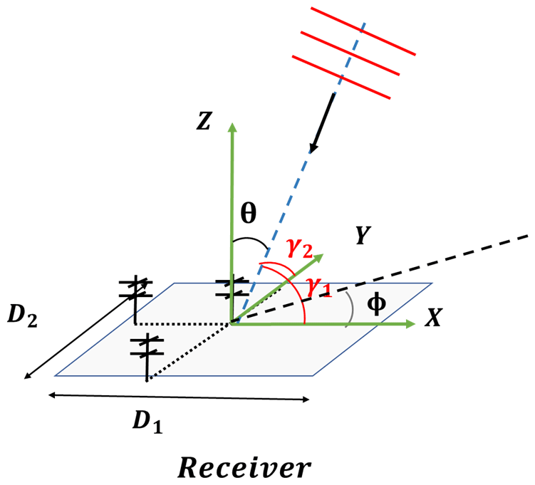
In coordinate XYZ, AoAs includes zenith angle θ and azimuth angle ϕ. In the plane wave approximation, the radio wave is at angle γ₁ and γ₂ with an antenna array (Fig. A2). There is a phase difference ΔΨ₁ and ΔΨ₂ between two antennas (Fig. 1). ΔΨ₁ and ΔΨ₂ can be expressed as follows:

$$\begin{array}{}\text{(A5)}& {\displaystyle }& {\displaystyle }\mathrm{\Delta }{\mathrm{\Psi }}_{\mathrm{1}}={\displaystyle \frac{\mathrm{2}\mathit{\pi }{D}_{\mathrm{1}}\cos {\mathit{\gamma }}_{\mathrm{1}}}{\mathit{\lambda }}},\text{(A6)}& {\displaystyle }& {\displaystyle }\mathrm{\Delta }{\mathrm{\Psi }}_{\mathrm{2}}={\displaystyle \frac{\mathrm{2}\mathit{\pi }{D}_{\mathrm{2}}\cos {\mathit{\gamma }}_{\mathrm{2}}}{\mathit{\lambda }}}.\end{array}$$

Using γ₁, γ₂ the AoA can be expressed as follows:

$$\begin{array}{}\text{(A7)}& {\displaystyle }& {\displaystyle }{\cos }^{\mathrm{2}}{\mathit{\gamma }}_{\mathrm{1}}+{\cos }^{\mathrm{2}}{\mathit{\gamma }}_{\mathrm{2}}+{\cos }^{\mathrm{2}}\mathit{\theta }=\mathrm{1},\text{(A8)}& {\displaystyle }& {\displaystyle }\tan \mathit{\varphi }={\displaystyle \frac{\cos {\mathit{\gamma }}_{\mathrm{2}}}{\cos {\mathit{\gamma }}_{\mathrm{1}}}},\end{array}$$

or in another expression:

$$\begin{array}{}\text{(A9)}& {\displaystyle }& {\displaystyle }\cos {\mathit{\gamma }}_{\mathrm{1}}=\sin \mathit{\theta }\cos \mathit{\varphi },\text{(A10)}& {\displaystyle }& {\displaystyle }\cos {\mathit{\gamma }}_{\mathrm{2}}=\sin \mathit{\theta }\sin \mathit{\varphi },\end{array}$$

substitute cos γ₁ and cos γ₂ in Eqs. (A7) and (A8) by using Eqs. (A5) and (A6):

$$\begin{array}{}\text{(A11)}& {\displaystyle }& {\displaystyle }{\cos }^{\mathrm{2}}\mathit{\theta }=\mathrm{1}-{\left({\displaystyle \frac{\mathit{\lambda }}{\mathrm{2}\mathit{\pi }}}\right)}^{\mathrm{2}}\left({\displaystyle \frac{{\mathrm{\Delta }}^{\mathrm{2}}{\mathrm{\Psi }}_{\mathrm{1}}}{D_{\mathrm{1}}^{\mathrm{2}}}}+{\displaystyle \frac{{\mathrm{\Delta }}^{\mathrm{2}}{\mathrm{\Psi }}_{\mathrm{2}}}{D_{\mathrm{2}}^{\mathrm{2}}}}\right),\text{(A12)}& {\displaystyle }& {\displaystyle }\ln \left(\tan \mathit{\varphi }\right)=\ln \left(D_{\mathrm{1}}\mathrm{\Delta }{\mathrm{\Psi }}_{\mathrm{2}}\right)-\ln \left(D_{\mathrm{2}}\mathrm{\Delta }{\mathrm{\Psi }}_{\mathrm{1}}\right).\end{array}$$

Equations (A11) and (A12) link the phase difference with the AoA and expanding θ and ϕ, ΔΨ₁ and ΔΨ₂ to the first order.

$$\begin{array}{}\text{(A13)}& {\displaystyle }\begin{array}{rl}& \mathrm{2}\cos \mathit{\theta }\sin \mathit{\theta }\mathit{\delta }\mathit{\theta }\\ & ={\left({\displaystyle \frac{\mathit{\lambda }}{\mathrm{2}\mathit{\pi }}}\right)}^{\mathrm{2}}\cdot \left[{\displaystyle \frac{\mathrm{2}\mathrm{\Delta }{\mathrm{\Psi }}_{\mathrm{1}}\mathit{\delta }\left(\mathrm{\Delta }{\mathrm{\Psi }}_{\mathrm{1}}\right)}{D_{\mathrm{1}}^{\mathrm{2}}}}+{\displaystyle \frac{\mathrm{2}\mathrm{\Delta }{\mathrm{\Psi }}_{\mathrm{2}}\mathit{\delta }\left(\mathrm{\Delta }{\mathrm{\Psi }}_{\mathrm{2}}\right)}{D_{\mathrm{2}}^{\mathrm{2}}}}\right]\end{array}\text{(A14)}& {\displaystyle }\mathit{\delta }\mathit{\varphi }={\displaystyle \frac{\sin \mathit{\varphi }\cos \mathit{\varphi }}{\mathrm{\Delta }{\mathrm{\Psi }}_{\mathrm{2}}}}\mathit{\delta }\left(\mathrm{\Delta }{\mathrm{\Psi }}_{\mathrm{2}}\right)-{\displaystyle \frac{\sin \mathit{\varphi }\cos \mathit{\varphi }}{\mathrm{\Delta }{\mathrm{\Psi }}_{\mathrm{1}}}}\mathit{\delta }\left(\mathrm{\Delta }{\mathrm{\Psi }}_{\mathrm{1}}\right)\end{array}$$

For Eqs. (A13) and (A14), substitute ΔΨ₁ and ΔΨ₂ using Eqs. (A5), (A6) and (A9), (A10) to the functions of θ, ϕ. Now Eqs. (3) and (4) have been proven. If the zenith angle $\mathit{\theta }=\mathrm{0}{}^{\circ }$, we stipulate that $\frac{\cos \mathit{\varphi }}{\sin \mathit{\theta }}$ and $\frac{\sin \mathit{\varphi }}{\sin \mathit{\theta }}$ are 1.

A3 Radial distance measuring error

Expanding R_s, R and cos α in Eq. (1) to the first order, δR_s can be expressed as a function of δR and δ(cos α):

$$\begin{array}{}\text{(A15)}& \begin{array}{rl}\mathit{\delta }{R}_{\mathrm{s}}& ={\displaystyle \frac{R^{\mathrm{2}}-\mathrm{2}Rd\cos \mathit{\alpha }+d^{\mathrm{2}}}{\mathrm{2}(R-d\cos \mathit{\alpha }{)}^{\mathrm{2}}}}\mathit{\delta }R\\ & +{\displaystyle \frac{d(R^{\mathrm{2}}-d^{\mathrm{2}})}{\mathrm{2}(R-d\cos \mathit{\alpha }{)}^{\mathrm{2}}}}\mathit{\delta }\left(\cos \mathit{\alpha }\right),\end{array}\end{array}$$

where α is the angle between R_s and the X_i axis. We denote the zenith and azimuth angles in coordinate X_iY_iZ_i as θ^′ and ϕ^′, respectively. The relationship between α and θ^′, i.e., ϕ^′, is

$$\begin{array}{}\text{(A16)}& \cos \mathit{\alpha }=\sin {\mathit{\theta }}^{\prime }\cos {\mathit{\varphi }}^{\prime }.\end{array}$$

Using the coordinate rotation matrix ${\mathbf{A}}_{\mathbf{R}}({\mathit{\psi }}_x^{X,i},{\mathit{\psi }}_y^{Y,i},{\mathit{\psi }}_z^{Z,i})$ and $\sin {\mathit{\theta }}^{\prime }\cos {\mathit{\varphi }}^{\prime }$ can be expressed as the function of AoA:

$$\begin{array}{}\text{(A17)}& \begin{array}{rl}\sin {\mathit{\theta }}^{\prime }\cos {\mathit{\varphi }}^{\prime }& =A_{\mathrm{11}}\sin \mathit{\theta }\cos \mathit{\varphi }+A_{\mathrm{12}}\sin \mathit{\theta }\sin \mathit{\varphi }\\ & +A_{\mathrm{13}}\cos \mathit{\theta }.\end{array}\end{array}$$

A_ij represent the elements in matrix ${\mathbf{A}}_{\mathbf{R}}({\mathit{\psi }}_x^{X,i},{\mathit{\psi }}_y^{Y,i},{\mathit{\psi }}_z^{Z,i}$) for $i,j=\mathrm{1},\mathrm{2},\mathrm{3}$.

Using Eqs. (A16) and (A17), δ(cos α) can be expressed as a function of δθ and δϕ as follows:

$$\begin{array}{}\text{(A18)}& \begin{array}{rl}& \mathit{\delta }\left(\cos \mathit{\alpha }\right)\\ & =(A_{\mathrm{11}}\cos \mathit{\theta }\cos \mathit{\varphi }+A_{\mathrm{12}}\cos \mathit{\theta }\sin \mathit{\varphi }-A_{\mathrm{13}}\sin \mathit{\theta })\mathit{\delta }\mathit{\theta }\\ & +(-A_{\mathrm{11}}\sin \mathit{\theta }\sin \mathit{\varphi }+A_{\mathrm{12}}\sin \mathit{\theta }\cos \mathit{\varphi })\mathit{\delta }\mathit{\varphi }.\end{array}\end{array}$$

Finally, δR_s can be expressed as the function of $\mathit{\delta }R,\mathit{\delta }\mathit{\theta },\mathit{\delta }\mathit{\varphi }$ as follows.

$$\begin{array}{}\text{(A19)}& \begin{array}{rl}\mathit{\delta }{R}_{\mathrm{s}}=& F(\mathit{\delta }R,\mathit{\delta }\mathit{\theta },\mathit{\delta }\mathit{\varphi })=f_R(\mathit{\theta },\mathit{\varphi })\mathit{\delta }R+f_{\mathit{\theta }}(\mathit{\theta },\mathit{\varphi })\mathit{\delta }\mathit{\theta }\\ & +f_{\mathit{\varphi }}(\mathit{\theta },\mathit{\varphi })\mathit{\delta }\mathit{\varphi }\end{array}\end{array}$$

$$\begin{array}{}\text{(A20)}& \begin{array}{rl}& f_R(\mathit{\theta },\mathit{\varphi })=\\ & {\displaystyle \frac{d^{\mathrm{2}}+R^{\mathrm{2}}-\mathrm{2}Rd(A_{\mathrm{11}}\sin \mathit{\theta }\cos \mathit{\varphi }+A_{\mathrm{12}}\sin \mathit{\theta }\sin \mathit{\varphi }+A_{\mathrm{13}}\cos \mathit{\theta })}{\mathrm{2}{\left[R-d(A_{\mathrm{11}}\sin \mathit{\theta }\cos \mathit{\varphi }+A_{\mathrm{12}}\sin \mathit{\theta }\sin \mathit{\varphi }+A_{\mathrm{13}}\cos \mathit{\theta })\right]}^{\mathrm{2}}}}\end{array}\end{array}$$

$$\begin{array}{}\text{(A21)}& \begin{array}{rl}& f_{\mathit{\theta }}(\mathit{\theta },\mathit{\varphi })=\\ & {\displaystyle \frac{d(R^{\mathrm{2}}-d^{\mathrm{2}})(A_{\mathrm{11}}\cos \mathit{\theta }\cos \mathit{\varphi }+A_{\mathrm{12}}\cos \mathit{\theta }\sin \mathit{\varphi }-A_{\mathrm{13}}\sin \mathit{\theta })}{\mathrm{2}{\left[R-d(A_{\mathrm{11}}\sin \mathit{\theta }\cos \mathit{\varphi }+A_{\mathrm{12}}\sin \mathit{\theta }\sin \mathit{\varphi }+A_{\mathrm{13}}\cos \mathit{\theta })\right]}^{\mathrm{2}}}}\end{array}\end{array}$$

$$\begin{array}{}\text{(A22)}& \begin{array}{rl}& f_{\mathit{\varphi }}(\mathit{\theta },\mathit{\varphi })=\\ & {\displaystyle \frac{d(R^{\mathrm{2}}-d^{\mathrm{2}})(-A_{\mathrm{11}}\sin \mathit{\theta }\sin \mathit{\varphi }+A_{\mathrm{12}}\sin \mathit{\theta }\cos \mathit{\varphi })}{\mathrm{2}{\left[R-d(A_{\mathrm{11}}\sin \mathit{\theta }\cos \mathit{\varphi }+A_{\mathrm{12}}\sin \mathit{\theta }\sin \mathit{\varphi }+A_{\mathrm{13}}\cos \mathit{\theta })\right]}^{\mathrm{2}}}}\end{array}\end{array}$$

A4 True error of E₂

The total length of side AC and side AB represents the pulse width. Side AC equals side CB and they are both equal to half of the pulse width S. In X_iY_iZ_i, the presentation of point A is $(x_i,y_i,z_i)$, the receiver is (0,0,0) and T_i is (d,0,0). The distance between T_i and A is $R_i=R-R_{\mathrm{s}}$. We denote the presentation of point B and C in X_iY_iZ_i as $(x_B,y_B,z_B)$ and $(x_C,y_C,z_C)$, respectively. We use vector collinear to establish equations for B and C. Therefore, one can obtain the coordinates of point B and C by the following equations:

$$\begin{array}{}\text{(A23)}& (x_B,y_B,z_B{)}^{\mathrm{T}}={\displaystyle \frac{R_{\mathrm{s}}-S}{R_{\mathrm{s}}}}(x_i,y_i,z_i{)}^{\mathrm{T}},\end{array}$$

$$\begin{array}{}\text{(A24)}& (x_C-d,y_C,z_C{)}^{\mathrm{T}}={\displaystyle \frac{R_i-S}{R_i}}(x_i-d,y_i,z_i{)}^{\mathrm{T}}.\end{array}$$

For isosceles triangle ABC, the perpendicular line AD intersects side CB at the midpoint D. Thus, we obtain the coordinate value of D in X_iY_iZ_i as follows:

$$\begin{array}{}\text{(A25)}& \begin{array}{rl}(x_D,y_D,z_D)=& {\displaystyle \frac{\mathrm{1}}{\mathrm{2}}}(x_B+x_c,y_B+y_c,z_b+z_c)\\ =& {\displaystyle \frac{\mathrm{1}}{\mathrm{2}}}\left(\right(a_{\mathrm{1}}+a_{\mathrm{2}})x_i-a_{\mathrm{2}}d\\ & +d,(a_{\mathrm{1}}+a_{\mathrm{2}}),y_i(a_{\mathrm{1}}+a_{\mathrm{2}})z_i).\end{array}\end{array}$$

We denote $a_{\mathrm{1}}=\frac{R_{\mathrm{s}}-S}{R_{\mathrm{s}}}$, $a_{\mathrm{2}}=\frac{R_i-S}{R_i}$. Finally, one can obtain the error vector of E₂ as vector DA in X_iY_iZ_i:

$$\begin{array}{}\text{(A26)}& \begin{array}{rl}\mathit{D}\mathit{A}=(& {\displaystyle \frac{(\mathrm{2}-a_{\mathrm{1}}-a_{\mathrm{2}})x_i+d(a_{\mathrm{2}}-\mathrm{1})}{\mathrm{2}}},{\displaystyle \frac{\mathrm{2}-a_{\mathrm{1}}-a_{\mathrm{2}}}{\mathrm{2}}}{y}_i,\\ & {\displaystyle \frac{\mathrm{2}-a_{\mathrm{1}}-a_{\mathrm{2}}}{\mathrm{2}}}{z}_i{)}^{\mathrm{T}}.\end{array}\end{array}$$

A5 Calculate AoA and range information in X_iY_iZ_i

For a space point $(x_i,y_i,z_i)$ in X_iY_iZ_i, which represents a MTSP, R_s can be solved easily as follows:

$$\begin{array}{}\text{(A27)}& \begin{array}{rl}& R_{\mathrm{s}}=(x_i,y_i,z_i)\\ & R_{\mathrm{s}}=\sqrt{x_i^{\mathrm{2}}+y_i^{\mathrm{2}}+z_i^{\mathrm{2}}}.\end{array}\end{array}$$

The distance between transmitter T_i and receiver R_X is d_i, as shown in Fig. 4a. Thus, the coordinate value of T_i in X_iY_iZ_i is $(d_i,\mathrm{0},\mathrm{0})$, and R_i can be solved as follows:

$$\begin{array}{}\text{(A28)}& R_i=\sqrt{(x_i-d_i{)}^{\mathrm{2}}+y_i^{\mathrm{2}}+z_i^{\mathrm{2}}}.\end{array}$$

Before we calculate the AoAs in X_iY_iZ_i, the representation of unit vectors of the x, y and z axes in X_iY_iZ_i needs to be known. In XYZ those unit vectors are easily represented as $(\mathrm{1},\mathrm{0},\mathrm{0}{)}^{\mathrm{T}}$, $(\mathrm{0},\mathrm{1},\mathrm{0}{)}^{\mathrm{T}}$, $(\mathrm{0},\mathrm{0},\mathrm{1}{)}^{\mathrm{T}}$. Through the coordinate rotation matrix ${\mathbf{A}}_{\mathbf{R}}({\mathit{\psi }}_x^{X,i},{\mathit{\psi }}_y^{Y,i}$,${\mathit{\psi }}_z^{Z,i})$, one can get those unit vector's representation in X_iY_iZ_i as follows:

$$\begin{array}{}\text{(A29)}& \begin{array}{r}{\mathit{n}}_{\mathit{x}}=(A_{\mathrm{11}},A_{\mathrm{21}},A_{\mathrm{31}}{)}^{\mathrm{T}}\\ {\mathit{n}}_{\mathit{y}}=(A_{\mathrm{12}},A_{\mathrm{22}},A_{\mathrm{32}}{)}^{\mathrm{T}}\\ {\mathit{n}}_{\mathit{z}}=(A_{\mathrm{13}},A_{\mathrm{23}},A_{\mathrm{33}}{)}^{\mathrm{T}}.\end{array}\end{array}$$

n_x, n_y and n_z are unit vectors of the x, y and z axes, respectively, and A_ij is the element's 3×3 matrix ${\mathbf{A}}_{\mathbf{R}}({\mathit{\psi }}_x^{X,i},{\mathit{\psi }}_y^{Y,i}$,${\mathit{\psi }}_z^{Z,i}$) for $i,j=\mathrm{1},\mathrm{2},\mathrm{3}$. Now the AoA can be obtained as follows:

$$\begin{array}{}\text{(A30)}& {\displaystyle }& {\displaystyle }\cos \mathit{\theta }={\displaystyle \frac{{\mathit{R}}_{\mathbf{s}}}{R_{\mathrm{s}}}}\cdot {\mathit{n}}_{\mathit{z}},\text{(A31)}& {\displaystyle }& {\displaystyle }\sin \mathit{\theta }=\sqrt{\mathrm{1}-{\cos }^{\mathrm{2}}\mathit{\theta }},\text{(A32)}& {\displaystyle }& {\displaystyle }\cos \mathit{\varphi }={\displaystyle \frac{{\mathit{R}}_{\mathbf{s}}}{R_{\mathrm{s}}}}\cdot {\displaystyle \frac{{\mathit{n}}_{\mathit{x}}}{\sin \mathit{\theta }}},\text{(A33)}& {\displaystyle }& {\displaystyle }\sin \mathit{\varphi }={\displaystyle \frac{{\mathit{R}}_{\mathbf{s}}}{R_{\mathrm{s}}}}\cdot {\displaystyle \frac{{\mathit{n}}_{\mathit{y}}}{\sin \mathit{\theta }}},\end{array}$$

for $\mathrm{0}{}^{\circ }<\mathit{\theta }<\mathrm{180}{}^{\circ }$ and $\mathrm{0}{}^{\circ }\le \mathit{\varphi }<\mathrm{360}{}^{\circ }$. When $\mathit{\theta }=\mathrm{0}{}^{\circ }$, we handle it the way as same as in Sect. A2.