On the estimation of boundary layer heights: a machine learning approach

The planetary boundary layer height (z_i) is a key parameter used in atmospheric models for estimating the exchange of heat, momentum, and moisture between the surface and the free troposphere. Near-surface atmospheric and subsurface properties (such as soil temperature, relative humidity, etc.) are known to have an impact on z_i. Nevertheless, precise relationships between these surface properties and z_i are less well known and not easily discernible from the multi-year dataset. Machine learning approaches, such as random forest (RF), which use a multi-regression framework, help to decipher some of the physical processes linking surface-based characteristics to z_i. In this study, a 4-year dataset from 2016 to 2019 at the Southern Great Plains site is used to develop and test a machine learning framework for estimating z_i. Parameters derived from Doppler lidars are used in combination with over 20 different surface meteorological measurements as inputs to a RF model. The model is trained using radiosonde-derived z_i values spanning the period from 2016 through 2018 and then evaluated using data from 2019. Results from 2019 showed significantly better agreement with the radiosonde compared to estimates derived from a thresholding technique using Doppler lidars only. Noteworthy improvements in daytime z_i estimates were observed using the RF model, with a 50 % improvement in mean absolute error and an R² of greater than 85 % compared to the Tucker method z_i. We also explore the effect of z_i uncertainty on convective velocity scaling and present preliminary comparisons between the RF model and z_i estimates derived from atmospheric models.

1 Introduction

Measuring the growth of the planetary boundary layer (PBL) height is crucial for understanding the turbulent transfer of air mass, which in turn strongly influences the winds, temperature, and moisture within the atmospheric boundary layer. During daytime, the air within the PBL is well mixed due to convection and results in weakening of turbulence at the top of the PBL (entrainment zone). One of the characteristics of the top of the PBL during clear-sky conditions is that the turbulence is near zero, while in cases with boundary layer clouds, significant up- and downdrafts can be observed at the top of the boundary layer (typically the cloud base height). Routine, continuous, long-term monitoring of the PBL height, z_i, is crucial for evaluating climate, weather, and air quality model skill in representing near-surface turbulent mixing, entrainment across the PBL top, the development of shallow cumulus, understanding effects of morning or evening transitions (Grant, 1997), and nocturnal convection initiation (Reif and Bluestein, 2017). Profiles of potential temperature, water vapour mixing ratio, and particulate concentration often exhibit strong gradients at or near the top of the PBL. Typically, estimates of z_i are obtained from an analysis of temperature and humidity profiles obtained from radiosondes. Indeed, radiosondes continue to be the de facto standard due to their long operational history, fine vertical resolution, accuracy, and reliability. However, major limitations are the poor temporal resolution and large sampling error because radiosondes are typically only launched twice daily at operational centres around the world. The launch time periods are generally not optimal for looking at various boundary layer properties. As a result, the diurnal variation in z_i is usually poorly represented in radiosonde data.

Modern remote sensing instruments can provide continuous estimates of the boundary layer dynamics. Space-based remote sensing instruments, such as Moderate Resolution Imaging Spectroradiometer, Tropical Rainfall Measuring Mission data and Multiangle Imaging SpectroRadiometer have also shown the ability to estimate PBL height (Wood and Bretherton, 2004; Karlsson et al., 2010).

Ground-based lidar systems, such as the Raman lidars (Turner et al., 2014), ceilometer, micro-pulse lidar (Campbell et al., 2002), atmospheric emitted radiance interferometer (Knuteson et al., 2004; Sawyer and Li, 2013), Doppler lidar (Tucker et al., 2009; Berg et al., 2017; Bonin et al., 2018; Vakkari et al., 2015; Banakh et al., 2021), and high-spectral-resolution lidar, have been commonly used to provide PBL height estimates (Quan et al., 2013; McNicholas and Turner, 2014). For elastic lidar systems such as the micro-pulse lidar, z_i is estimated by locating the height where the range-corrected signal-to-noise ratio (SNR) or attenuated backscatter profile experiences a strong decrease with height (Emeis et al., 2008). A similar approach is used to estimate z_i from profiles of water vapour mixing ratio from Raman lidar (Summa et al., 2013) or differential absorption lidar systems (Hennemuth and Lammert, 2006); however, the peak in the water vapour variance has also been used as an estimate of z_i (Turner et al., 2014).

Doppler lidars provide range-resolved measurements of radial velocity, attenuated backscatter, and SNR. When staring vertically, a ground-based Doppler lidar measures height-resolved profiles of vertical velocity in the lower atmosphere with a temporal resolution of 1 s or less. Profiles of the vertical velocity variance can then be computed by averaging over an appropriate time interval (typically 15 to 30 min). The primary advantage of Doppler lidars is that they measure the turbulence directly and thus provide a more defensible measure of z_i. Other systems rely on gradients of aerosol loading or moisture that are used to infer z_i.

One method for estimating the convective boundary layer (CBL) depth using Doppler lidars is to find the height where the vertical velocity variance profile falls below some prescribed threshold, which in some cases can vary with time (Lenschow et al., 2000; Tucker et al., 2009; Lenschow et al., 2012; Berg et al., 2017). This method, which we refer to as the Tucker method, is simple to implement and provides a direct measure of z_i. However, the estimates are sensitive to the choice of variance threshold, which is somewhat arbitrary. Also, this method fails under stable nocturnal conditions due to weak turbulence and the fact that the lowest gate of the lidar is often above the depth of the nocturnal z_i. Horizontal velocity variance and dissipation rate profiles from a Doppler lidar can be used to estimate z_i in nocturnal conditions (Vakkari et al., 2015; Banakh et al., 2021). Alternatively, one can estimate the PBL height based on wind shear and turbulence kinetic energy (TKE), but there has been limited research on this topic (Brost and Wyngaard, 1978; Teixeira and Cheinet, 2004; LeMone et al., 2018).

Due to different measurement approaches between multiple remote sensing instruments, considerable uncertainties exist when comparing z_i to standard radiosonde retrievals. PBL heights from different instruments provide expected trends during certain atmospheric conditions (mostly daytime convective time periods) but differ slightly due to measurement uncertainties and thresholds chosen associated with each instrument. Therefore, a framework independent of threshold techniques used in previous studies is warranted. Although this paper does not directly address a unified approach to estimate z_i, it is a step in that direction.

In view of these limitations, we investigate the potential of using a machine learning (ML) approach for continuous monitoring of z_i, with a focus on CBL. ML enables us to bring together various observations to arrive at a consensus answer. ML models, such as RF and neural networks, have been used for classifying various atmospheric phenomena (McGovern et al., 2017; Gagne et al., 2019; Vassalo et al., 2020) or retrieving atmospheric variables (e.g. Solheim et al., 1998; Cadeddu et al., 2009). The RF model is versatile, simple to implement, and robust. Training the RF model entails providing it with observations (i.e. features) that aid in predicting z_i. Examples of such observations include surface sensible and latent heat flux, soil temperature, soil moisture, surface potential temperature, surface humidity, etc. These features have all been shown to exhibit some degree of correlation with z_i (Santanello et al., 2005; Zhang et al., 2013).

Here we use a RF model to predict z_i using input features derived from vertically staring Doppler lidar data and various surface and sub-surface observations. We use a multi-year dataset from the U.S. Department of Energy (DOE)'s Southern Great Plains (SGP) site (Sisterson et al., 2016) for training and evaluating the RF model. Reference z_i measurements from radiosondes are used in the RF training process (Sivaraman et al., 2013). Specifically, the RF model is trained using observations from 2016 through 2018, and its performance is evaluated using data from 2019.

In this paper, Sect. 2 describes the observations that are used in this study, and Sect. 3 describes the details of the RF model, including the training method, data conditioning, and performance. Results of the RF model's performance are presented in Sect. 4, and in Sect. 5 we examine how RF model-derived z_i estimates affect the scaling of the vertical velocity variance profiles. PBL height estimates from Energy Exascale Earth System Model (E3SM) Atmosphere Model version 1 (EAMv1), large-eddy simulations (LESs), and observations are compared in Sect. 6. Finally, a summary and future work are provided in Sect. 7.

2 Data sources

The U.S. DOE Atmospheric Radiation Measurement (ARM) User Facility operates the SGP site in north-central Oklahoma (Mather and Voyles, 2013; Sisterson et al., 2016). The site contains an extensive suite of instrumentation for monitoring the atmosphere and surface properties. Most of these instruments operate continuously, and the data are freely available from the ARM website (https://adc.arm.gov/discovery, last access: 5 May 2020; McCord and Voyles, 2016). The SGP site contains several heavily instrumented subsites or “facilities” that are geographically dispersed over Oklahoma and Kansas (Mather and Voyles, 2013). For this study, we use observations from the central facility (C1), which also contains the largest number and most diverse suite of instruments in ARM. Figure 1 shows the layout of the SGP C1 site and the locations of instruments used in this study. Additionally, Table 1 lists the instruments, ARM data stream names, and specific measurements that were used. In ML, independent variables, or inputs, are often referred to as features. A model can have multiple features/inputs and for this project, the measurements from the observations will be referred to as features in the RF model.

Figure 1 ARM SGP site C1 layout and instruments used in this study in Oklahoma, USA. Maps are extracted from © Google Earth and © Google Maps.

Table 1 Instruments, ARM data stream names, and measurements used in this study.

The ARM User Facility has operated a Halo Photonics Stream Line XR (Pearson et al., 2009) at C1 since April 2011. The instrument provides height- and time-resolved measurements of radial velocity, attenuated backscatter, and SNR. The range resolution is set to 30 m and the temporal resolution is about 1 s. The instrument is configured to stare vertically most of the time. Once every 15 min, it executes a plan-position-indicator scan, from which profiles of the wind speed and direction are computed. The vertical staring data are used to compute profiles of noise-corrected vertical velocity variance using a 30 min averaging period. More details about the instrument are provided by Newsom and Krishnamurthy (2020). Details about the vertical velocity statistics value-added product (VAP) are provided by Newsom et al. (2019b), and details about the Doppler lidar wind VAP are given by Newsom et al. (2019a).

Doppler-lidar-derived features used in this study are listed in Table 1. The list includes raw height-resolved measurements of attenuated backscatter and range-corrected SNR, which are known to be directly correlated with z_i (Cohn and Angevine, 2000; Brooks, 2003). Also listed are several derived quantities such as cloud base height, wind shear, turbulence eddy dissipation rate, and z_i estimated using the Tucker method (Tucker et al., 2009). Typically, the nocturnal vertical velocity variance estimates are too small, and the threshold used in the Tucker method is not applicable. During certain rare nocturnal convection initiation events, larger vertical velocity variance estimates are observed and the same threshold (0.04 m² s⁻²) is used to estimate nighttime values of z_i from the lidar. For consistency in terminology being used here, we refer to all z_i estimates from the lidar as the Tucker method (both nighttime and daytime). Because the range of the Doppler lidars at SGP C1 is often less than 1 km (see Appendix A), estimates of eddy dissipation rate (using 1 Hz vertical velocity stares; Champagne et al., 1977) above 800 m were affected by system noise. Thus, features such as the eddy dissipation rate, attenuated backscatter, and SNR from the Doppler lidar were limited to 800 m a.g.l. Reducing the height from 800 to 500 m a.g.l. did not impact the results. Moreover, RF models used in this study are only capable of ingesting one-dimensional time series data; therefore, two-dimensional Doppler lidar features were averaged over the vertical column (90 m (lowest range gate) to 800 m a.g.l.). Adding these features increased the overall variance explained by the RF model (82 % of the total variance compared to 74 % of the total variance without using lidar-derived parameters).

The ARM PBL VAP (sgppblhtsonde1mcfarlC1.c1) contains estimates of z_i derived from radiosondes launched at SGP C1. We note that radiosondes are typically launched four times daily from SGP C1, nominally at 0530, 1130, 17:30, and 23:30 UTC each day (local time = UTC−6). The PBL VAP uses three different algorithms for estimating z_i. These include the Heffter (1980), two bulk Richardson thresholds methods, and Liu and Liang (2010). The Heffter (1980) method is a well-established and widely used algorithm (e.g. Marsik et al., 1995; Delle Monache et al., 2004) that determines z_i from potential temperature gradients using criteria related to the strength of an inversion and the potential temperature difference across the inversion. The bulk Richardson number (Ri_b) is a dimensionless number relating vertical stability to vertical shear. It represents the ratio of thermally produced turbulence to that generated by vertical shear. Methods using Ri_b to estimate z_i assume that there is no turbulence production at the top of the stable boundary layer, and therefore Ri_b exceeds its critical value at the top of the boundary layer (Seibert et al., 2000). Several different critical thresholds of Ri_b are provided in the literature based on resolution of sondes, location, etc. The ARM PBL VAP includes z_i estimates based on two critical thresholds (0.25 and 0.5). Liu and Liang (2010) provide different thresholds for estimating convective and stable boundary layer depths using potential temperature profiles. The inversion strength thresholds used in the method varies for given stability regime and land type classification (land, ocean, or ice). We note that the various estimates can differ considerably. More details about the ARM PBL VAP are provided by Sivaraman et al. (2013).

Preliminary data analysis

Boundary layer height estimation algorithms (Tucker et al., 2009; Berg et al., 2017; Bonin et al., 2018) purely using the Doppler lidars are limited by the range of the Doppler lidars at the ARM SGP facility, which may or may not reach the top of the boundary layer. The data availability of the ARM Doppler lidar SGP C1 systems is typically less than 1–2 km (Newsom and Krishnamurthy, 2020), and the data availability of the Doppler lidar vertical stares and velocity azimuth display scans for the study period are shown in Appendix A. The Tucker method z_i is used for inter-comparison with the RF model in this study, primarily due to its ease in application to the multi-year dataset and known performance, including its established usage in studies using the ARM Doppler lidar and other locations and instruments (Träumner et al., 2011; Shukla et al., 2014; Schween et al., 2014; Berg et al., 2017; Lareau et al., 2018; Lareau, 2020). Vertical velocity variance profiles provided in the sgpdlprofwstats4newsC1.c1 VAP and a variance threshold of 0.04 m² s⁻² are used to determine z_i, following Tucker et al. (2009). The results are somewhat sensitive to the choice of threshold such that the z_i estimates decrease as the threshold is increased (Berg et al., 2017).

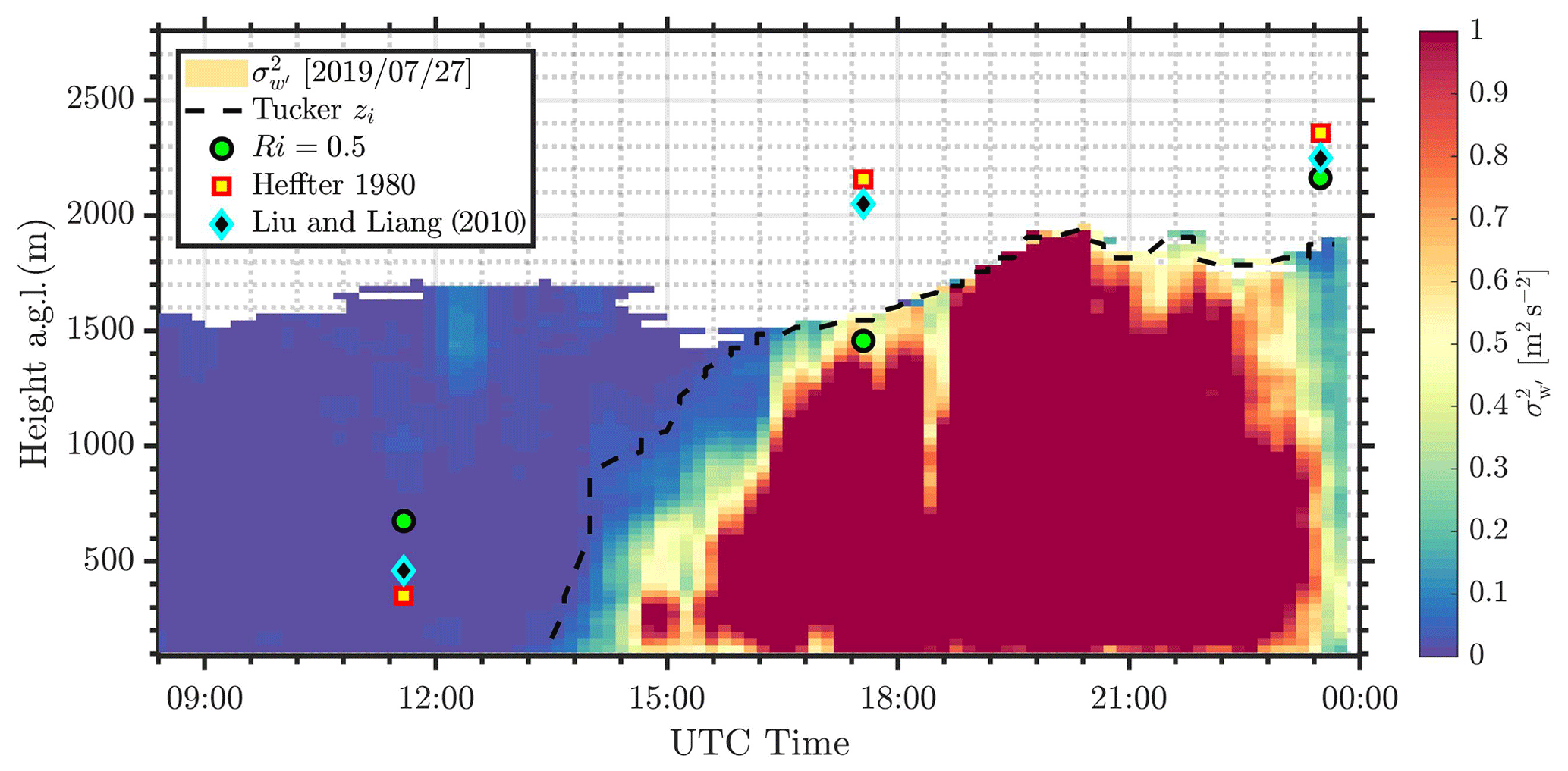
Figure 2 Typical CBL showing lidar variance (colours), Tucker z_i (black line), and radiosonde z_i (three methods; symbols). The horizontal axis shows the number of hours after 00:00 UTC on 27 July 2019.

Figure 2 shows a typical example of vertical velocity variance during the warm season at SGP. Also shown are estimates of z_i from the Tucker method. We find that the Tucker method generally works well at tracking the height of the convective mixed layer during its initial development phase and can be made to match the radiosonde observations by changing the vertical velocity variance threshold (Schween et al., 2014). In that case, there is sufficient SNR for the lidar to see both the developing convection and the overlying residual layer. However, as the mixed layer continues to deepen, at some point the SNR becomes too small to enable reliable estimates of the vertical velocity variance. This problem is sometimes compounded by a slight reduction in sensitivity during the hottest portion of the day, which we suspect is the result of strong refractive turbulence in the surface layer. Although this effect has not been thoroughly analysed due to lack of refractive turbulence profiles and concurrent radiosonde data, there could be instances when the Doppler lidar is indeed measuring the top of the boundary layer. In any event, the loss of signal near the CBL top could result in z_i estimates from the Tucker method being low biased.

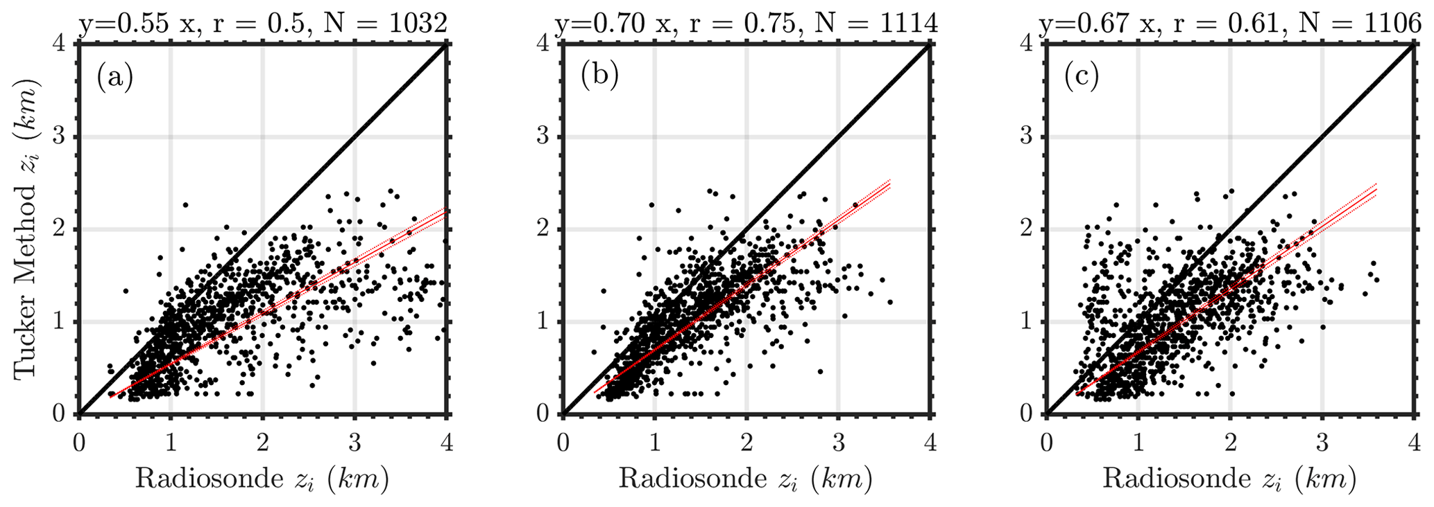
Figure 3 Comparisons between Tucker method and three different z_i estimates from radiosondes. (a) Heffter (1980), (b) Liu and Liang (2010), and (c) bulk Richardson number method using a threshold of 0.5. The red line is the best fit with the fit y=mx shown above. r is the correlation coefficient, and N is the total number of radiosonde and Tucker method observations used in each scatter plot.

For this study, radiosonde-derived z_i estimates are used to calibrate the RF algorithm. Figure 3 shows comparisons between lidar-derived CBL (using the Tucker method) and simultaneous estimates from the ARM PBL VAP. These comparisons were performed using 1785 cases with radiosonde data and daytime clear (identified as periods when surface heat flux is positive from sunrise to sunset and cloud base height is zero) or shallow cumulus conditions (identified as cloud base height less than 5 km from Doppler lidar and cloud fraction less than 0.1) for the years 2016 through 2019. From these results, we found that the Liu and Liang (2010) technique resulted in the best overall agreement with the Tucker method z_i, in terms of the correlation coefficients (r=0.75) and slope (0.70). Thus, z_i estimates from the Liu–Liang technique in the ARM PBL VAP (pblhtsonde1mcfarl.c) are used as a reference to calibrate the RF model in this study. It should be noted that any of the above three model outputs can be used to calibrate the ML model, if needed, and the choice could vary with each site. For a different site, we would recommend conducting a similar correlation analysis as shown above with various radiosonde models and lidar data to determine the optimal model for RF calibration. It is important to note that during stable conditions, the determination of z_i from radiosondes is very uncertain, as the turbulence can result from either buoyancy forcing or wind shear, and the radiosonde rapidly rises through the relatively thin stable boundary layer. At SGP C1, the nose of the low-level jet can also be used to define the height of the boundary layer (Sivaraman et al., 2013). Therefore, the focus of this study is to only demonstrate the ability of the RF model to replicate nighttime z_i estimates compared to radiosonde-derived values. We hope this framework developed in this article can be adapted easily to future research in estimating the true stable boundary layer height from radiosondes or other reference sources. During stable conditions, the true z_i can be below the lowest range gate of the Doppler lidar, and we expect such a technique would aid in representing true z_i estimates with proper calibration.

3 Machine learning

In this study, an RF algorithm was used to predict PBL heights. RF regression (Breiman, 2001) is an ensemble method that is made up of a population of decision or decorrelated trees. Figure 4 provides a graphical illustration of the RF bootstrapping process. Bootstrap aggregation (bagging) is used so that each RF tree (a sample is shown in Appendix B) can randomly sample from an entire feature set, while only a subset of the total feature set is given to each individual tree. For example, if the entire feature set contains say M different features, an individual RF tree can contain a fraction of those M features. The premise behind RF is to improve the variance reduction of bagging by reducing the correlation between the trees without increasing the variance. The trees can be truncated to add further diversification. After construction, the population's individual predictions are averaged to give a final prediction of the target variable. Ideally, this process results in a diversified and decorrelated set of trees whose predictive errors cancel out, producing a more robust final prediction.

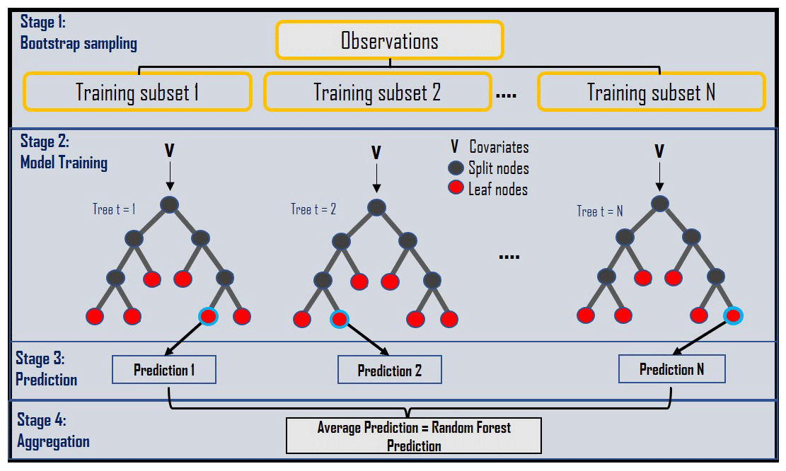
Figure 4 Graphical representation of a standard RF algorithm (adapted from online sources and Fig. A1).

An advantage of RFs is their ability to determine the importance of all input features for the predictive process. This is done by calculating the mean decrease in impurity or the decrease in variance that is achieved during a given split in each decision tree. The decrease in impurity for each input feature can be averaged over the entire forest, providing an approximation of the feature's importance for the prediction (feature importance estimates sum to 100 % to ease interpretability). A sample regression tree developed by real data used in this article is shown in Appendix B (Fig. B1). The statistics and ML toolbox in MATLAB contain all the functions needed to build the RF algorithm used in this study.

3.1 Model hyperparameters

In this study, a least-squares boosting regression (LSboost) ensemble RF model (Breiman, 2001) is built based on observational data listed in Table 1. At every iteration, the ensemble fits a new decision tree to minimize the mean-squared error between the observed response and the aggregated prediction of all decision trees developed previously. The MATLAB function fitrensemble is used to develop the RF model. The algorithm creates several regression trees using a subset of input features and radiosonde observations. The RF model creates a learning process to map the reference data to input features. Hyperparameters are used to control the learning process in the RF model. It is good practice to tune hyperparameters such as the maximum number of decision splits per tree (see Fig. 4), learn rate for shrinkage, and the number of iterations for reducing the generalization error (Breiman, 2001). In this article, hyperparameters for the RF model are chosen by performing a Bayesian optimization on the data, which minimizes the k-fold cross validation loss function for select hyperparameters (MATLAB function bayesopt). For this study, three hyperparameters were optimized: the number of tree splits, number of learning cycles or iterations, and learn rate for the model. Based on the optimization results, the number of iterations was set to 460, number of tree splits to 11, and learning rate to 0.25 for the current model.

Regularization techniques are used to prevent statistical overfitting in a predictive model (Hastie et al., 2009), by reducing the magnitude of the coefficients of the RF model for certain parameters that do not contribute to the target variable. In general, regularization algorithms can treat issues such as multicollinearity and redundant predictors and make the model more precise. The MATLAB function regularize is used for the regularization process, which is based on the Lasso regularization algorithm (Tibshirani, 1996). This regularization algorithm optimizes the number of trees and avoids data overfitting.

3.2 Data preprocessing

Surface and lidar data from 2016 to 2019 are used in this analysis. ARM VAPs provide processed and quality-controlled data from several atmospheric sensors. Each VAP provides quality control thresholds that are used to filter the data. For example, the lidar VAPs (DLWSTATS and DLWIND) provide quality control flags based on the system noise and SNR (Newsom and Krishnamurthy, 2020). For this analysis, thresholds specified in the VAPs are used to remove any erroneous data. Similarly, quality control flags for all variables mentioned in Table 1 above are used to filter bad data (Tang et al., 2019). Because the temporal resolution of the surface data are variable, measurements are interpolated or averaged to the lidar 15 min resolution time stamps. The frequency of radiosondes is generally 6 h at SGP but can be in intervals of 3 h during select field campaigns (Mather et al., 2018). For training purposes, surface and lidar data to the nearest radiosonde observations within 15 min are chosen.

Normalizing, standardizing, and scaling processes are used to scale the variables in an ML model, such that they have the same order of magnitude in their value. Standardizing involves aligning the features to have a zero mean and scaled to have a standard deviation of 1. Typically, RF models do not need standardizing or normalizing features due to the inherent bagging process (Breiman, 2001). At SGP C1, large diurnal variability was observed for certain parameters (like TKE, dissipation rate, etc.), leading to a large distribution of values between daytime and nighttime. This skewed the number of trees the RF model builds for daytime and nighttime estimates. Standardizing the features showed improvements while estimating nocturnal z_i estimates from the RF model. Therefore, to improve nocturnal z_i estimates, standardized datasets will be used in the following analysis for all conditions.

All the features, listed in Table 1, are filtered based on ARM mentor guidelines for each instrument and then normalized. These measurements are fed into an ensemble RF model using the hyperparameters described above. Once the RF model is built, a lasso regularization approach is used on the RF model to limit the effect of collinearity on the target variable. Similar to a least-squares regression, collinear columns tend to deteriorate the accuracy of the output (Krishnamurthy et al., 2013; Yoo et al., 2014). Once the RF model is built, it can be used to estimate z_i for time periods that are not being used to train the model. In MATLAB, this is typically done using the predict function.

Table 2 Data imputation evaluation and performance on boundary layer heights for the year 2019.

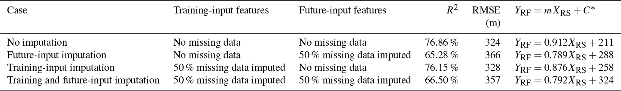
^∗ RF – random forest; RS – radiosondes.

The RF model is trained using sub-surface, surface, lidar, and concurrent radiosonde z_i data from 2016, 2017, and 2018. From here on, these data are referred to as training-input features. A total of 3919 radiosonde z_i measurements were used in the training process. The 2019 sub-surface, surface, and lidar data are referred to as future-input features and are used to provide an independent dataset to evaluate the trained RF method. From an operational perspective, missing input features are quite common. The most common approach is to fill in (impute) the missing features (Hastie et al., 2009). Surrogate data using a local median of the nearest 10 data points are used in the analysis (Hastie et al., 2009). Other imputation algorithms such as k-nearest neighbour were also tested, and similar results were observed. It is critical for the RF model to deal with missing values in its training phase. In some cases, the added noise in the system can help improve the stability of the RF model. But too much noise is also detrimental in the training process, and the imputed data may no longer be useful and can cause erroneous results. The imputation process is done inherently during the RF bagging process. The effect of data imputation on model performance was evaluated by training the RF model with and without data imputation. Four different possibilities in evaluating the performance of the RF model with and without imputation are evaluated, as shown in Table 2. In the case of no imputation (no missing data), only time periods when all features/parameters are available are used in the RF regression. In the case of 50 % missing data, approximately 50 % of the time series data were missing (at random) due to say issues with data quality, and surrogate data were used. The choice of 50 % was to mimic a worst-case real-world scenario based on experience, where either one or two instruments from the feature set of 20 odd variables have data quality issues. Other combinations, such as no missing data used in the RF regression during the training process and 50 % future-input feature missing data and vice versa, were evaluated.

As can be seen from Table 2, data imputation overall reduces the accuracy of RF model performance. Missing future-input features seems to have the highest effect on the RF model z_i estimates, regardless of training the model based on missing training-input features. This could be due to several reasons, such as the fact that the median value does not represent the current state of the missing data, the same input features are not missing in both training and future input features as the combinations to test are near infinite (as the data in real-world scenarios can be missing in random as in the case above), etc. Assessing the performance of the RF algorithm using data imputation creates an additional level of complexity when one of the features is missing for a given time step compared to others. For example, if the relative humidity feature is missing for a given time step and lidar measurements are missing for another time step, the effect on the RF model output is not similar. The RF model provides weights to each feature, and the impact on the RF model would be dependent on the calibration and ability of the imputation algorithm to estimate the missing value. Since there are several possible scenarios here (as we have close to 20 odd features), and capturing all errors effectively would be a challenge, each feature is not weighted equally in the model. Therefore, in this analysis, the model is trained with no missing data, and no imputation is done on the data (either input or future features) to accurately test the efficacy of the RF model. The authors would like to note that the results in Sect. 4 are in some sense optimistic due to the treatment of missing data, and the worst-case performance of such an algorithm must be thoroughly evaluated. Future studies are planned to implement a better imputation model based on data from past trends for a given feature and to test RF model performance.

RF models are generally site specific; initial tests (not shown) show the possibility to develop a generalized RF model to estimate z_i for all sites around SGP (C1 and other satellite sites) with good accuracy under all atmospheric conditions. A round-robin-type analysis, where a model developed at a given site is tested at every other site and vice versa, would be a valuable exercise (Bodini and Optis, 2020).

4 Performance of RF z_i

Boundary layer height predictions from the RF model and Tucker method were compared to radiosonde estimates. Mean absolute error (MAE) is defined as

$$\begin{array}{}\text{(1)}& \mathrm{MAE}={\displaystyle \frac{\mathrm{1}}{N}}\sum _{i=\mathrm{1}}^N\left|z_{i\mathrm{RS}}-z_{i\mathit{\gamma }}\right|,\end{array}$$

where z_iRS is the boundary layer height estimated from the radiosondes (Liu and Liang, 2010), and z_iγ is the boundary layer height estimated from either the Tucker method or RF model. The root-mean-square error (RMSE) is defined as

$$\begin{array}{}\text{(2)}& \mathrm{RMSE}=\sqrt{{\displaystyle \frac{\mathrm{1}}{N}}\sum _{i=\mathrm{1}}^N{\left(z_{i\mathrm{RS}}-z_{i\mathit{\gamma }}\right)}^{\mathrm{2}}}.\end{array}$$

Similarly, the linear correlation coefficient (R) is defined as

$$\begin{array}{}\text{(3)}& R={\displaystyle \frac{\mathrm{1}}{{\mathit{\sigma }}_{\mathrm{RS}}{\mathit{\sigma }}_{\mathit{\gamma }}(N-\mathrm{1})}}\sum _{i=\mathrm{1}}^N\left(z_{i\mathrm{RS}}-z_{\mathrm{RS}}\right)\left(z_{i\mathit{\gamma }}-z_{\mathit{\gamma }}\right),\end{array}$$

where z_RS and z_γ denote the mean of radiosonde and RF or Tucker method boundary layer heights, respectively, σ_RS and σ_γ denote their standard deviations, and N denotes the number of samples.

Table 3 Systematic mean absolute errors, root-mean-square error, and correlation coefficient (R²) between RF, Tucker method, and radiosonde z_i estimates in 2019.

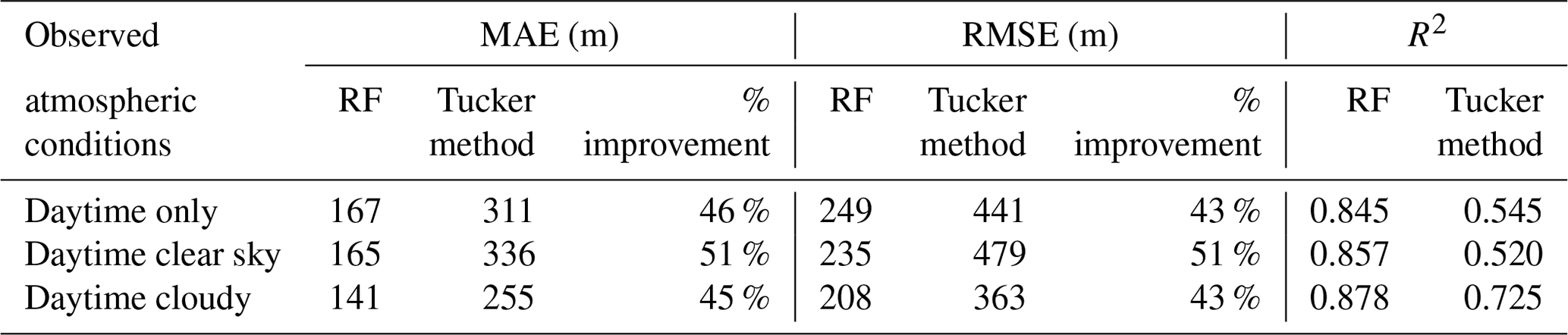
MAE and RMSE for the daytime atmospheric conditions from Tucker and RF methods are shown in Table 3. Daytime is defined as the period when surface heat flux is positive (i.e. sunrise to sunset), clear sky is defined as time periods when no clouds are observed from the Doppler lidar (with an hourly cloud fraction less than 0.1), and cloudy conditions are defined as time periods when clouds below 5 km are observed from the Doppler lidar (with an hourly cloud fraction greater than 0.1). It can be observed that the RF method shows considerable improvements compared to the Tucker method for all three categories. Improvements of 40 %–50 % in MAE and RMSE are observed under various conditions. The least improvement in RF z_i estimates is observed during cloudy conditions, with a MAE improvement of 45 % compared to the Tucker method. Correlation coefficients are also observed to improve significantly during all daytime conditions.

Due to the presence of a nocturnal low-level jet (LLJ) at SGP, all seasons, the radiosonde nighttime z_i estimates are generally below the LLJ height and are well tracked by the RF model (see Sect. 4.1). A comparison of nocturnal RF model z_i estimates with other remote sensing devices that continuously monitor the boundary layer height needs to be conducted (e.g. Raman lidar) and is a part of future work.

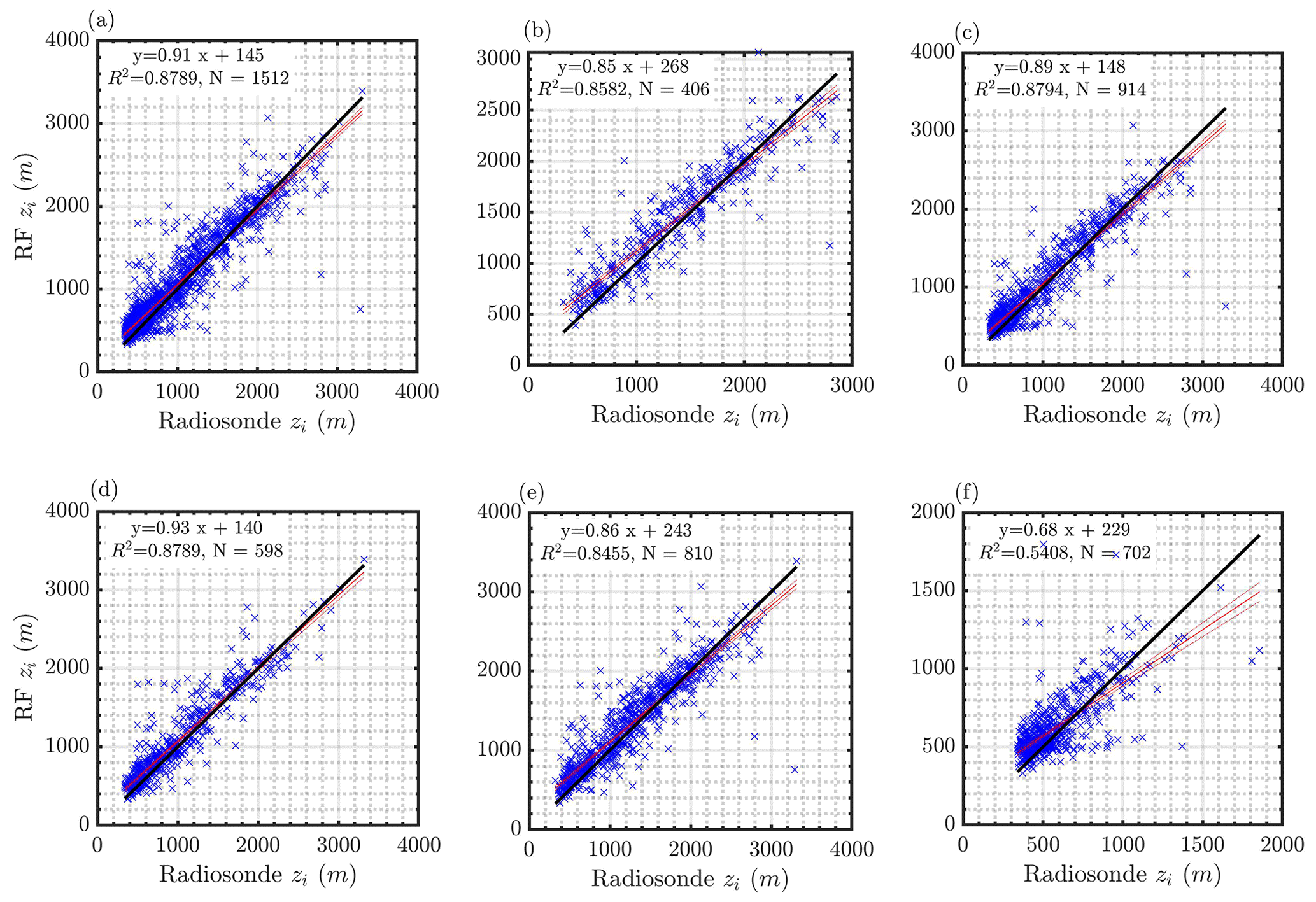
Figure 5 Correlations between RF PBL height and radiosonde PBL height for (a) all data in 2019, (b) daytime clear sky, (c) clear-sky daytime and nighttime, (d) cloudy daytime and nighttime, (e) daytime only, and (f) nighttime only.

Nocturnal estimates of z_i from radiosondes at SGP are much more uncertain (Sivaraman et al., 2013). Regardless of the accuracy of the z_i estimate from radiosondes, the ability of the RF model to predict the input data is evaluated. Consequently, the data were split into five atmospheric conditions: (1) daytime and clear sky (26 %), (2) day and night clear sky (60 %), (3) day and night cloudy (40 %), (4) daytime only (53 %), and (5) nighttime only (46 %). Although some cases overlap in the above situations, the idea was to evaluate the RF model performance reasonably during both daytime, nighttime, cloudy, and clear-sky condition combinations. These five atmospheric conditions were chosen, because these are commonly observed atmospheric conditions at SGP and have been observed to have an impact on z_i (e.g. variations in cloud base height varies z_i). The associated correlation plots between RF z_i estimates and corresponding radiosonde z_i estimates are shown in Fig. 5. Overall, the RF model z_i estimates correlate well with radiosonde z_i, with an R² of greater than 0.85 during all the above conditions. During clear-sky conditions (including both daytime and nighttime), RF z_i estimates show the highest correlation of 0.88. Although the sample size varied for five categories, the correlation coefficients are overall high for the RF z_i estimates (compared to Tucker method in Fig. 3). During the night, the z_i values from the radiosondes are relatively constant, and the RF estimates are consistent with these values. However, due to the small dynamic range of the nighttime z_i values, the correlation between the radiosonde and RF methods is relatively poor (0.54). Based on the slopes of the regression lines in Fig. 5, the RF model tends to overestimate z_i when it is small and slightly underestimate z_i when it is large. Possible reasons for this trend are under further investigation.

Overall, a uniform improvement in z_i can be obtained using RF techniques. Reducing or increasing the training data had an impact on the RF model performance, but the increase in the magnitude of the correlation coefficient was negligible using at least 2 years of data. In this analysis, 3 years of data were used for training the RF model.

4.1 Time series and diurnal and seasonal performance

The RF model was trained using data from 2016 to 2018, and z_i estimates for 2019 were estimated using the parameters listed in Table 1. The temporal resolution of the RF model z_i estimates is 15 min. Figures 6 and 7 show lidar z_i estimates from the Tucker method, radiosondes, and RF model on 20 and 22 June 2019, respectively. Cloud base height and vertical velocity variance profiles from Doppler lidar are also overlaid. Due to an ongoing field campaign, the micropulse differential absorption lidar demonstration project, these days observed a higher frequency of radiosonde observations (Weckworth et al., 2020). It is clear that the RF model z_i closely follows radiosonde z_i estimates, and the Tucker method underestimates z_i as estimated from radiosondes. Although the Tucker method is observed to track the convective boundary layer height effectively, a bias is observed when compared to the radiosonde z_i. Optimizing the vertical velocity variance thresholds could potentially reduce the bias in certain conditions, but the bias is not uniform across all time periods (see Fig. 7). Because aerosol concentration decreases with altitude, signal availability reduces as a function of height. During peak convection, when the aerosol concentration above the boundary layer is minimal, lidar measurements sometimes do not reach the top of the boundary layer with sufficient SNR to be detected. The lidar beam also attenuates considerably when it encounters clouds or fog due to increased atmospheric scattering or attenuation. In Fig. 6, it can also be seen that lack of aerosols limits the Doppler lidars' ability to measure above the boundary layer height during peak convective periods. During nighttime conditions, vertical velocity variance is low and is not effective in estimating z_i. In this study, the lowest range gate is used as the stable boundary layer height from the lidar as a first guess. As mentioned earlier, nocturnal conditions during summer months are dominated by southerly winds where the nocturnal boundary layer is capped by a low-level jet (Krishnamurthy et al., 2020). During these conditions, the RF model shows near-constant z_i, which is observed to be well correlated with radiosonde z_i (just below the LLJ height).

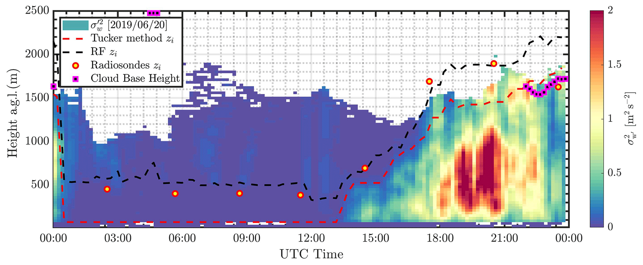
Figure 6 Boundary layer height estimates at the SGP central facility on 20 June 2019 from the Tucker method (Tucker et al., 2009), RF model z_i, radiosondes z_i (Sivaraman et al., 2013), cloud base height estimates from lidar (Newsom et al., 2019b), and the background colours represent vertical velocity variance measurements from Doppler lidar.

Figure 7 As in Fig. 6, but for 22 June 2019.

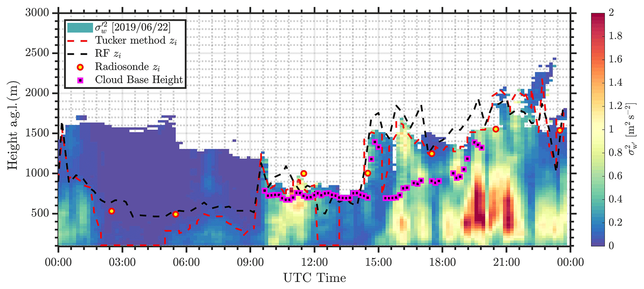
In Fig. 7, the effectiveness of the RF model can clearly be observed. At 03:00 and 06:00 UTC, during stable nocturnal conditions, the RF model matches the radiosonde estimates very well. At 09:00 UTC, a possible nocturnal convection initiation event results in high vertical velocity variance for several hours (Reif et al., 2017). Convection initiation refers to the process in which an air parcel is successfully lifted to its level of free convection and produces a precipitating updraft (Markowski and Richardson, 2010). The RF model is observed to detect that burst of convection and provide coherent boundary layer heights past 12:00 UTC until daytime transition at ∼ 14:00 UTC. The correlation between RF model and radiosonde z_i estimates is very high. Therefore, various atmospheric interaction effects are aptly characterized by the parameters in the RF model. Hourly averaged z_i and daily maximum z_i averaged for each season in 2019 from the Tucker method, RF model, and radiosondes are shown in Fig. 8a. Although the number of samples between the radiosondes and RF model estimates are vastly different, the generic trend in the hourly and seasonal boundary layer height variability is well captured by the RF model. Although the Tucker method captures the average boundary layer height trend, it shows a clear bias in convective boundary layer height estimates compared to radiosonde- and RF-model-derived z_i values. As observed earlier from the time series analysis, a standard bias correction would not always improve z_i estimates from the Tucker method. Daily daytime maximum z_i estimates averaged over four seasons in 2019 from all three methods are shown in Fig. 8b. Summer months (May through August) show high boundary layer heights. During these months, the peak convective period occurs during the daytime at around 20:00 UTC, and the average boundary layer height as observed from the RF model is ∼ 2100 m above ground level, which correlates well with radiosondes released during the same time period. During winter and autumn months, the peak convective period does not always occur at 20:00 UTC, and therefore the maximum z_i estimates from radiosondes do not coincide with RF estimates. The Tucker method invariably underestimates maximum z_i during all seasons.

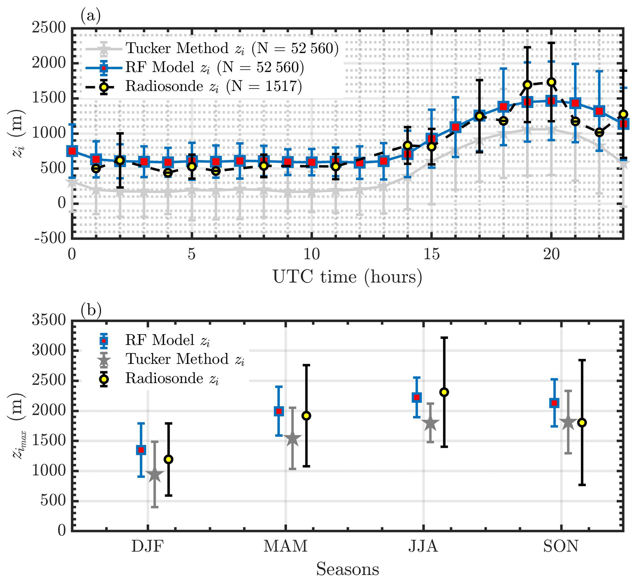
Figure 8 (a) Hourly averaged z_i estimates at the SGP central facility for 2019 from RF, the Tucker method, and radiosondes. Total number of samples (N) for each dataset is also shown in the legend. (b) Daily daytime maximum z_i estimates for four seasons (DJF, MAM, JJA, SON) from RF, radiosonde, and the Tucker method. The bars in both plots represent 1 standard deviation.

4.2 Input feature importance

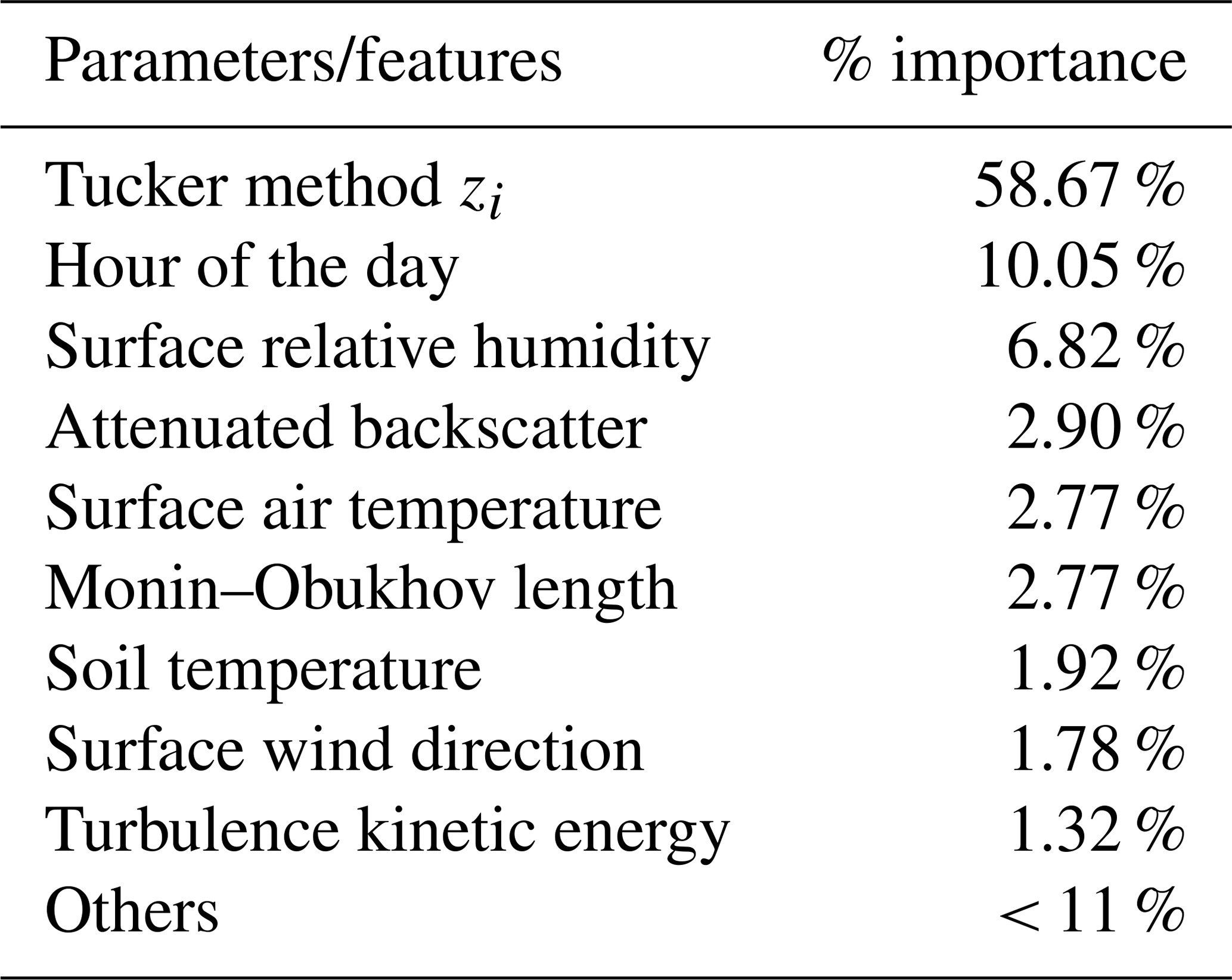
All the input features within the RF model explain approximately 82 % of the total variance in the data. Table 4 provides the unbiased predictor importance estimates, which is computed by permuting or shuffling a variable in the model and estimating its mean square error (Breiman, 2001). If a predictor is significant in prediction, then permuting its values will affect the model error and vice versa. However, if two input variables are highly correlated (as is expected when testing atmospheric forcing), it is highly unlikely that the reported importance values will accurately represent each variable's significance (Breiman, 2001). Based on this analysis, the most important parameter is the initial z_i guess from the Tucker method. This provides a very good first guess to the RF model, especially during convective conditions. Although the RF model is sensitive to the initial guess from the Tucker method, it is observed to be robust enough to ignore uneven spikes in z_i estimates due to noise in the lidar vertical velocity variance data (Fig. 7). The second most important feature observed to have high correlation with z_i estimate is the hour of the day. A clear diurnal pattern in z_i, i.e. higher values in the daytime and near-constant values during the nighttime, estimates is observed at SGP. Therefore, hour of the day can effectively classify the data, which is beneficial in the RF bagging process. Relative humidity also shows higher importance (> 5 %), where drier conditions are observed to have higher correlations with boundary layer height. Deep convection and larger z_i is generally a consequence of greater sensible heat flux and lower latent heat flux, which are primarily due to higher surface temperature and lower relative humidity. Based on an evaluation of z_i over Europe, it was also observed that relative humidity had a strong negative correlation with z_i, and surface temperature had a positive correlation (Zhang et al., 2013). Other features such as lidar attenuated backscatter, surface air temperature, Monin–Obukhov length, soil temperature, surface wind direction, and TKE are all observed to be important for accurately characterizing the boundary layer height at SGP. Other surface features such as surface friction velocity, sensible heat flux, longwave radiation, etc., have lower correlations with z_i within the RF model framework. Therefore, the model can be reduced to the list of parameters defined in Table 4 for optimal estimation of the boundary layer height at SGP.

Table 4 Key parameter/feature unbiased importance estimates during all conditions.

To assess the key features during nighttime, a similar RF model was built by conditionally sampling nighttime data. During nighttime, the key parameters that affect the RF model predictions are shown in Table 5. It is interesting to note that the key features deemed important during nighttime are significantly different compared to all conditions, and the percent importance is more evenly distributed across many features. This result alludes to the fact that nocturnal stable boundary layers are indeed complex to model, and several processes are at play (Fernando and Weil, 2010). Monin–Obukhov length is observed to have the highest impact on the nighttime RF model estimates and is consistent with theory on stable boundary layers (Zilitinkevich, 1972; Zilitinkevich and Baklanov, 2002). Although nighttime z_i initial guesses are generally a constant (lowest lidar range gate if no high vertical velocity variance is observed), the initial guess has shown to be effective in adjusting the RF model z_i estimates. Other local parameters such as soil temperature, surface air temperature, dew point temperature, longwave radiation, and turbulence kinetic energy are observed to be correlated with nighttime z_i estimates. One of the stable boundary layer models by Brost and Wyngaard (1978) is given by

$$\begin{array}{}\text{(4)}& z_i=\mathrm{0.4}{\left({\displaystyle \frac{u_{\ast }L}{\mathrm{|}f\mathrm{|}}}\right)}^{\mathrm{1}/\mathrm{2}},\end{array}$$

where u_∗ is the friction velocity, L is the Monin–Obukhov length, and f is the Coriolis parameter. As shown in Table 5, the nighttime parameters deemed important by the RF model include both Monin–Obukhov length and friction velocity. As discussed earlier, the dominant feature of nocturnal boundary layer at SGP is the presence of the LLJ. The turbulence production at SGP is not only influenced by surface characteristics but also heavily influenced by the presence of the LLJ. A preliminary comparison with the above model to RF model z_i estimates at SGP was very poor, as the radiosondes (from all three methods) invariably pick up the nocturnal LLJ at SGP as the height of the boundary layer. Although the height of the nocturnal boundary layer height could be debatable at SGP, the premise of this paper is to show the effectiveness of the RF model in tracking and detecting the boundary layer height and the input boundary layer height provided to the model. Further research needs to be conducted on providing widely acceptable nocturnal boundary layer height at SGP, and a trained RF model can provide continuous boundary layer height estimates even in nocturnal conditions with acceptable levels of accuracy.

Table 5 Key parameter/feature unbiased importance estimates during nighttime conditions.

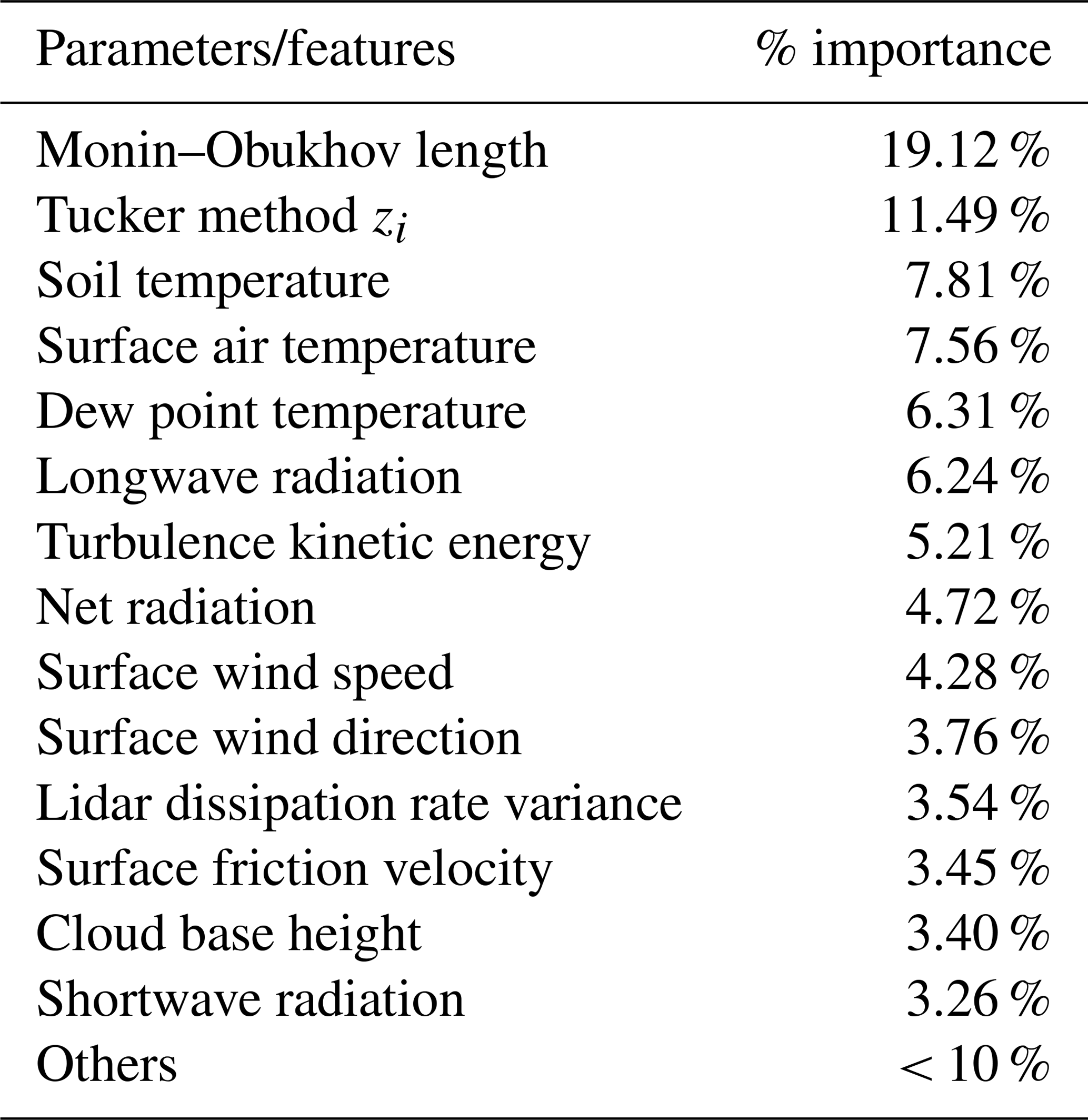
Figure 9 RF partial dependence during all conditions from (a) the Tucker method z_i, (b) relative humidity, (c) hour of the day, (d) Monin–Obukhov length, (e) surface wind direction, and (f) soil temperature to boundary layer height at the central facility. High dependence shows more sensitivity of the RF model to the bin of feature values.

The partial dependence of key features on z_i during all conditions is shown in Fig. 9. Partial dependence estimates show the marginal effect of features on the predicted outcome of an ML model. Therefore, a higher partial dependence estimate corresponds to higher sensitivity to the predicted outcome, in our case the boundary layer height and vice versa. From Fig. 9, we see that RF model z_i is sensitive to warmer soil temperatures, lower-relative-humidity conditions, daytime hours, higher z_i from the Tucker method, northerly wind directions, and stable atmospheric conditions. Most of these conditions would mimic dry convective conditions, with increased turbulence activity within the boundary layer. Monin–Obukhov length is observed to effectively categorize the training data into stable and unstable atmospheric conditions, with high partial dependence estimates during stable boundary layer conditions. Similar relationships can be derived for other parameters. It is important to note that the parameters shown to be important with respect to the RF model are features that successfully aid in the RF bagging process. Santenello et al. (2007) and Tang et al. (2018) showed parameters such as soil moisture and evaporative flux to be key variables in warm seasons, in a two-parametric regression framework, that affect boundary layer properties. Within the RF model, although those parameters are deemed important, soil temperature, lidar backscatter, and relative humidity were shown to have a higher impact on boundary layer height at each site.

In this research, the input features into the RF model are standard atmospheric parameters (such as wind speed, temperature, etc.). An alternate approach to this effort would be to provide several non-dimensional inputs (such as bulk Richardson number, Obukhov length scale, ratio of Brunt–Väisälä frequency to the Coriolis parameter, etc.) as inputs because they capture multiple dimensions of the data with a single variable (Vassallo et al., 2020, 2021). Because non-dimensional scaling is a common approach in atmospheric fluid dynamics to detect patterns in the data, a similar approach would provide the RF model with various relations and be helpful in classifying the data better. But further research needs to be conducted in defining the key nondimensional parameters that affect z_i at SGP and is a part of future work.

5 Normalized vertical velocity variance profiles

Within a convective boundary layer, vertical velocity variance profiles are often scaled by the convective velocity scale (w^∗), which is a function of z_i (Lenschow et al., 1980) for analysis. Therefore, any error in z_i estimates can result in altering the vertical velocity variance profiles. Herein, we attempt to estimate the effect of z_i on normalized vertical velocity variance profiles and convective velocity estimates, often used to compare results in boundary layer studies and in the functional relationships used in atmospheric models. The convective velocity scale is given as

$$\begin{array}{}\text{(5)}& w^{\ast }={\left[{\displaystyle \frac{g{z}_i\stackrel{\mathrm{‾}}{w^{\prime }{\mathit{\theta }}^{\prime }}}{\mathit{\theta }}}\right]}^{\mathrm{1}/\mathrm{3}},\end{array}$$

where g is the gravitational constant, θ is potential temperature, and $\stackrel{\mathrm{‾}}{w^{\prime }{\mathit{\theta }}^{\prime }}$ is heat flux. The heat flux is obtained from the surface eddy covariance system at SGP C1 (Cook, 2018a), and potential temperature is measured at 4 m. An uncertainty in z_i will cause a non-linear effect in the convective velocity scale estimates. Assume the uncertainty in z_i can be given as $z_i^{\prime }$, and the mean is given as $\stackrel{\mathrm{‾}}{z_i}$. The error caused in the convective velocity scale due to uncertainty in z_i can be formulated as shown below:

$$\begin{array}{}\text{(6)}& w^{\ast }={\left[{\displaystyle \frac{g\left(\stackrel{\mathrm{‾}}{z_i}+z_i^{\prime }\right)\stackrel{\mathrm{‾}}{w^{\prime }{\mathit{\theta }}^{\prime }}}{\mathit{\theta }}}\right]}^{\mathrm{1}/\mathrm{3}}.\end{array}$$

This can also be written as

$$\begin{array}{}\text{(7)}& w^{\ast }={\left[{\displaystyle \frac{g\stackrel{\mathrm{‾}}{z_i}\stackrel{\mathrm{‾}}{w^{\prime }{\mathit{\theta }}^{\prime }}}{\mathit{\theta }}}\right]}^{\mathrm{1}/\mathrm{3}}{\left(\mathrm{1}+{\displaystyle \frac{z_i^{\prime }}{\stackrel{\mathrm{‾}}{z_i}}}\right)}^{\mathrm{1}/\mathrm{3}}.\end{array}$$

Therefore, the convective velocity scale error due to uncertainty in z_i can be estimated using the term $(\mathrm{1}+x{)}^{\mathrm{1}/\mathrm{3}}$, where $x=\frac{z_i^{\prime }}{\stackrel{\mathrm{‾}}{z_i}}$. Based on observations at SGP C1, z_i from the Tucker method is observed to be negatively biased to radiosonde estimates. The ratio, $\left(\frac{z_i^{\prime }}{\stackrel{\mathrm{‾}}{z_i}}\right)$, is calculated using the median error between Tucker method and RF model z_i by the median z_i using the RF model. The ratio is calculated to be approximately −0.28 for data from 2016 to 2019. This would result in an uncertainty of approximately 10 % in the convective velocity estimates when Tucker method z_i values are used in the calculations. Although this is an average, during certain conditions (e.g. during transition time periods) the effect of poor characterization of z_i can be even larger. Figure 10 shows average vertical velocity variance profiles during convective time periods at SGP from 2015 to 2019 using z_i estimates from the Tucker method and RF model. Higher z_i values result in lower scaled vertical velocity variance estimates. Differences in variance profiles are observed to be smaller during daytime transition (15:00 UTC or 09:00 LT), as the Tucker method generally provides reliable z_i estimates. During peak convective conditions (20:00 UTC) and evening transition (23:00 UTC), as observed earlier, the Tucker method z_i estimates tend to diverge from radiosonde z_i depending on the scenario and are negatively biased. Overall, the error introduced in the scaled vertical velocity variance profiles due to Tucker method z_i is above 15 %.

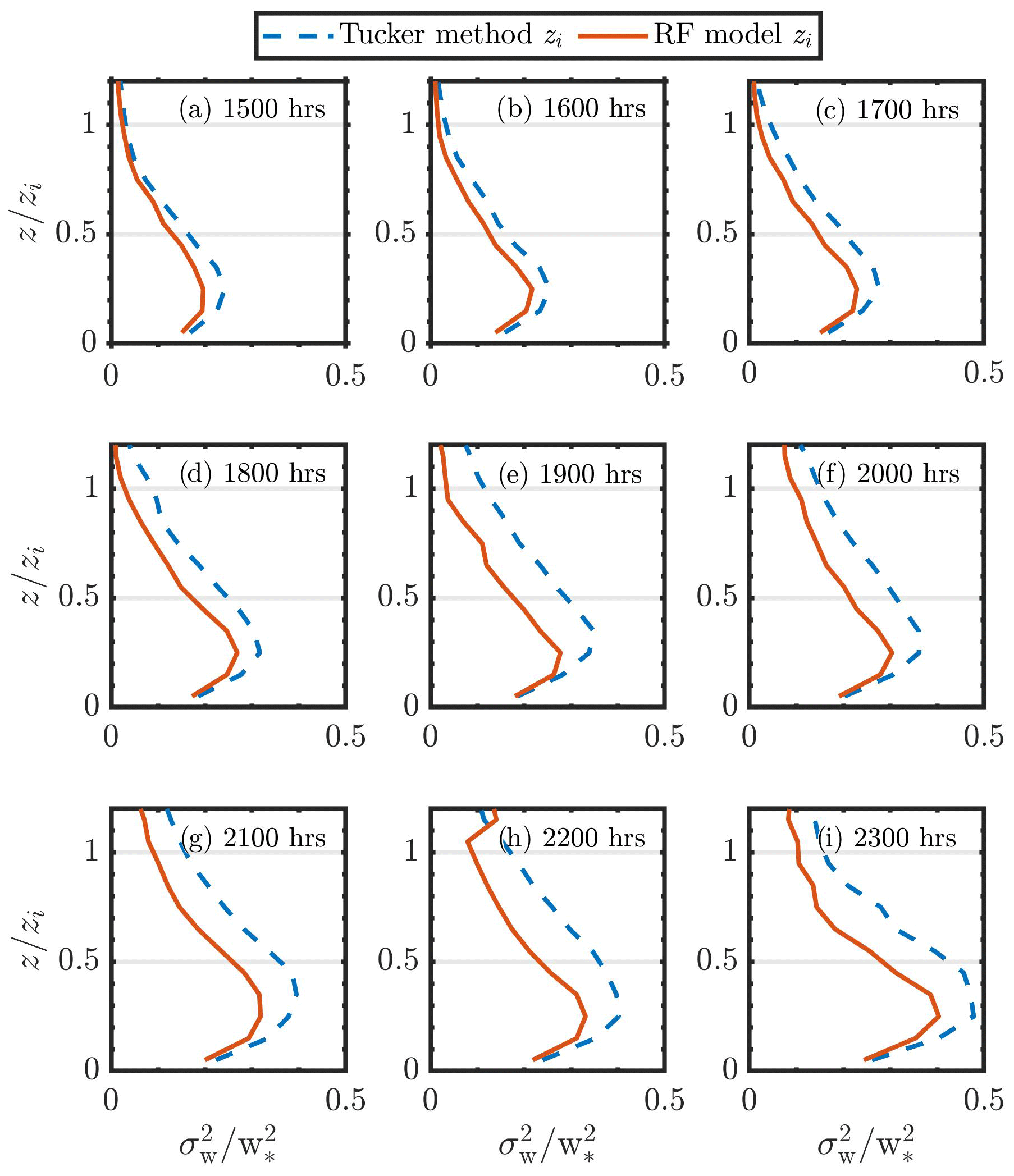
Figure 10 Average normalized vertical velocity variance profiles during convection periods (15:00 to 23:00 UTC, a–i) at SGP from 2015 to 2019 versus non-dimensional height using z_i estimated by the Tucker method and RF model. Appropriate z_i (RF model or Tucker method) was used in both x- and y-axis scaling.

As per definition, the turbulence at the top of the boundary layer is expected to be near zero, except during cloudy conditions. As shown in Fig. 10, during morning transition periods, when the lidar does measure above the boundary layer, the scaled vertical velocity variance profiles do converge to zero. In contrast, during peak convective conditions the scaled profiles do not converge to zero and are observed to have an offset of generally around 0.1 at z_i (also observed in Lareau et al., 2018). This could be due to higher uncertainty in lidar vertical velocity variance estimates near z_i, ineffective filtering of the lidar false alarm rates (Bouquet et al., 2016), uncertainty in surface in situ measurements, and the possibility of residual turbulence above the boundary layer during downdrafts or updrafts.

6 Case study: preliminary model comparisons

We expect the RF model z_i outputs to be developed into a VAP that will be easily accessible and can be used by researchers across the community. Therefore, the motivation for this case study is to provide a preliminary comparison between model-estimated z_i and the RF model z_i. These types of comparisons will help understand the impact of boundary layer properties on model physics and guide further in improving parameterizations used to represent boundary layer turbulence.

The surface and sub-surface layer measurements are key for understanding land–atmosphere interactions. Land–atmosphere interactions drive Earth's surface water and energy budgets. They can alter clouds and precipitation around a region, affect the growth of the planetary boundary layer height, and influence the persistence of extremes such as droughts. In view to better understand land–atmosphere interactions, a field campaign, Holistic Interactions of Shallow Clouds, Aerosols and Land Ecosystems (HI-SCALE), was conducted at the SGP site in Oklahoma (Fast et al., 2019). The field campaign was conducted from April to September of 2016, with two 4-week intensive observational periods in May and September. Simulations were conducted on select clear-sky days during the HI-SCALE field campaign. Two simulations using different modelling systems were performed: Energy Exascale Earth System Model (E3SM; Golaz et al., 2019) Atmosphere Model version 1 (EAMv1; Rasch et al., 2019) and a LES model. The Weather Research Forecasting (Skamarock et al., 2008) LES is set up in the same way as that used in operational LASSO (Gustafson et al., 2017, 2020). The Weather Research Forecasting model version used is v3.7. The model horizontal domain is square, doubly periodic, and 25.6 km wide with a 100 m horizontal grid spacing. The model top is set at 14.8 km above the surface. There are 226 vertical levels with a vertical grid spacing of ∼ 30 m in the lowest 5 km. The model is run for 15 h for each case day starting at 06:00 UTC. The Rapid Radiation Transfer Model for Global Climate Models parameterization is used for shortwave and longwave radiation (Clough et al., 2005; Iacono et al., 2008; Mlawer et al., 1997). The Thompson parameterization is used for microphysics (Thompson et al., 2004, 2008). The Deardorff 1.5-order turbulent kinetic energy approach is used for subgrid-scale parameterization (Deardorff, 1980). The model is initialized with ARM sounding from the SGP site (ARM user facility, 2001). The surface sensible and latent heat fluxes are horizontally uniform and prescribed from the ARM constrained variational analysis data product (ARM user facility, 2004). The large-scale forcing is also taken from the ARM variational analysis data product. Due to high computational expense, the LES model was run for 3 d while the EAMv1 model was run for the entire duration of the HI-SCALE campaign. The EAMv1 model is run in the standard coarse-resolution configuration with ∼ 1^∘ horizontal grid spacing and 72 vertical levels and a physics time step of 30 min and a cloud and turbulence time step of 5 min. In these models, z_i was estimated using resolved vertical velocity variance estimates from the LES or the parameterized vertical velocity estimate from the Cloud Layers Unified by Binormals (CLUBB) boundary layer parameterization applied in E3SM (Golaz et al., 2002; Larson and Golaz, 2005; Bogenshutz and Krueger, 2013; Larson, 2017), and like the Tucker method a low threshold was used to estimate the depth of the convective boundary layer. Estimates of boundary layer height from E3SM and LASSO were not made during nocturnal conditions. The LASSO simulations extend only from approximately sunrise to sunset, so nocturnal estimates of the boundary layer height are not possible. The E3SM simulations generally have too much nighttime turbulence, making estimates of the boundary layer height unreliable at night.

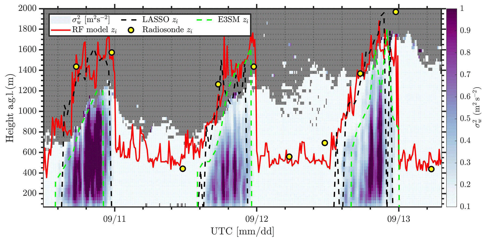
Figure 11 Vertical velocity variance (${\mathit{\sigma }}_{\mathrm{w}}^{\mathrm{2}}$) estimates from Doppler lidar for 3 d (10, 11, and 12 September 2016) with z_i estimates from (a) the RF model (red solid line), (b) radiosondes (yellow circles), (c) the LASSO model (black dashed line), and (d) the E3SM model (green dashed line).

Figure 11 shows Doppler lidar vertical velocity variance measurements for 3 d during the HI-SCALE campaign (10–12 September 2016) and boundary layer height estimates from RF model, radiosondes, LASSO, and E3SM. Because the RF model provides z_i estimates at a much finer temporal resolution than radiosondes, these estimates are ideal for comparing with models and assessing areas where model performance can be improved. Therefore, in this preliminary comparison, the primary motivation is to see if we can identify areas where the models diverge significantly by using near-continuous accurate z_i values from the RF model. Due to computational expense, we could evaluate only 3 d of model results, but further research is needed in performing a thorough evaluation.

Conditions on 10 September were relatively calm with northerly winds, and no clouds were observed during daytime. On 11 and 12 September, there were southerly winds and clear-sky conditions during both daytime and nighttime. Daytime maximum surface air temperature is observed to increase progressively from 10 to 12 September, and as mentioned earlier higher air temperature results in deeper planetary boundary layer due to increased convection (see Fig. 11).

Overall, the LES model compares better to RF estimates, while EAMv1 is observed to underestimate z_i. Due to the coarse resolution of EAMv1, ∼ 100 km, z_i estimates are averaged over a large domain and do not generally capture the fine-scale variability. Although the LES model is observed to pick up morning transition, it diverges from observations during evening transitional periods and does not capture the decay of turbulence accurately. During peak convective conditions, when the vertical velocity variance is large, the LES is observed to correlate very well with the RF model and radiosonde z_i. Although EAMv1 is observed to mostly underestimate z_i compared to RF model estimates, occasionally the model captures the peak convective trends. Like the LES model z_i, the EAMv1 is also not observed to capture evening decay of turbulence accurately but is observed to not track the early morning transition at SGP as well. Such systematic differences between the model and data are crucial for targeting future research directions. Further study is needed to evaluate the reasons why models tend to deviate during early morning and/or evening transition periods.

7 Summary

This study used a range of near-surface, sub-surface and Doppler lidar parameters to predict boundary layer heights at the ARM SGP site using an RF model. The RF model was trained using several years of data, and the model was validated with radiosonde estimates of boundary layer height. Because the Tucker method is observed to be low biased during peak convective periods due to low SNR of the Doppler lidars as the boundary layer deepens, the RF model corrects for the bias. Seasonal and diurnal variations in z_i as observed from radiosondes correlate well with RF model z_i. During convective boundary layer conditions, the mean absolute error of boundary layer height estimated by the RF model is reduced by almost 50 % compared to the Tucker method. Significant improvement was also observed during clear-sky and cloudy conditions. Nocturnal estimates from the RF model were not well correlated with radiosonde measurements, mostly due to near-constant estimates of nocturnal boundary layer height at SGP (due to the presence of the LLJ). Moreover, valuable information on the impact of surface parameters on nocturnal z_i estimates by the RF model provides avenues for further research in accurately estimating stable boundary layer heights at SGP. The key variables that have shown to have the largest impact on the RF model predictions are the initial guess of the boundary layer height from the Tucker method, hour of day, surface relative humidity, soil temperature, and attenuated backscatter (aerosol loading). During nocturnal conditions, several parameters, such as the Monin–Obukhov length, soil temperature, and surface air temperature, influence the RF model estimates. These parameters are aligned with theoretical parameterization schemes used to estimate boundary layer heights. The RF model used in this study explains around 82 % of the variance in the data at SGP C1.

Uncertainty in convective boundary layer heights results in more than 10 % difference in convective velocity scale estimates when the Tucker method is used. The uncertainty results in more than 15 % error in scaled velocity variance estimates, which are commonly used in atmospheric models. Limited comparison between microscale model z_i estimates of the RF model and radiosonde z_i values show increased correlation during heightened land–air interaction events. Large-eddy simulation estimates are observed to match the convective z_i variability as estimated by the RF model while the global model performance is variable. Neither model captures the evening transitional decay of turbulence accurately.

There are a number of ways to expand on the research presented here. Future work could focus on improved data imputation models to better handle missing data, a RF model z_i uncertainty framework using individual RF tree predictions, and finally a study of the effect of nearby wind farms and surface heterogeneity have on the boundary layer height.

Appendix A

The range availability of the ARM SGP C1 Doppler lidars used in this study is provided below. Figure A1 shows the height range and data availability at SGP C1 for vertical stare scans and Fig. A2 for processed velocity azimuth display (VAD) scans. The lidar range is consistent across multiple years of operation. The availability of data from the scanning Doppler lidars at SGP C1 is significantly reduced for altitudes greater 1 km (60 % availability), which could limit its ability to reach the top of the boundary layer during all conditions.

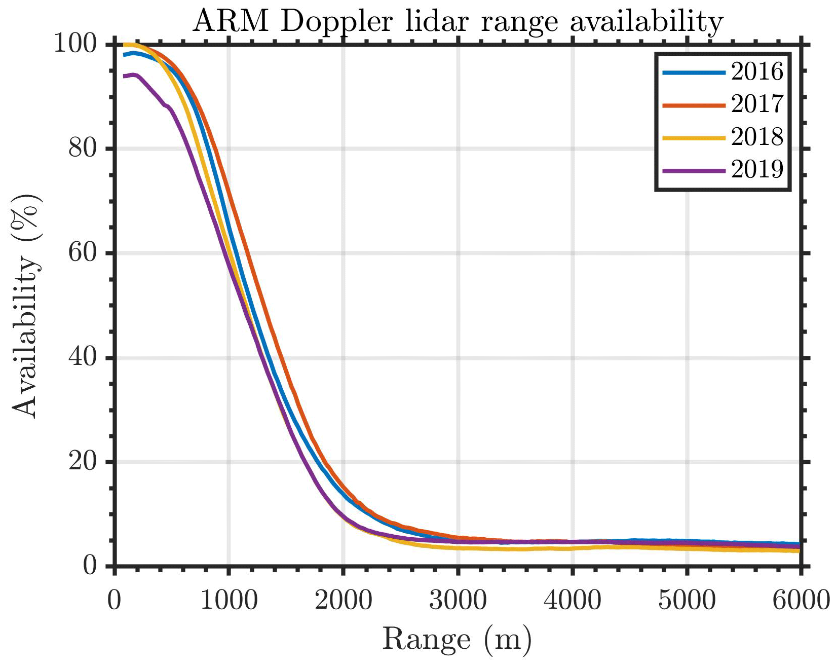
Figure A1 ARM SGP C1 Doppler lidar range availability versus range from vertical stares from 2016 to 2019 after SNR filtering (threshold of 1.008 dB).

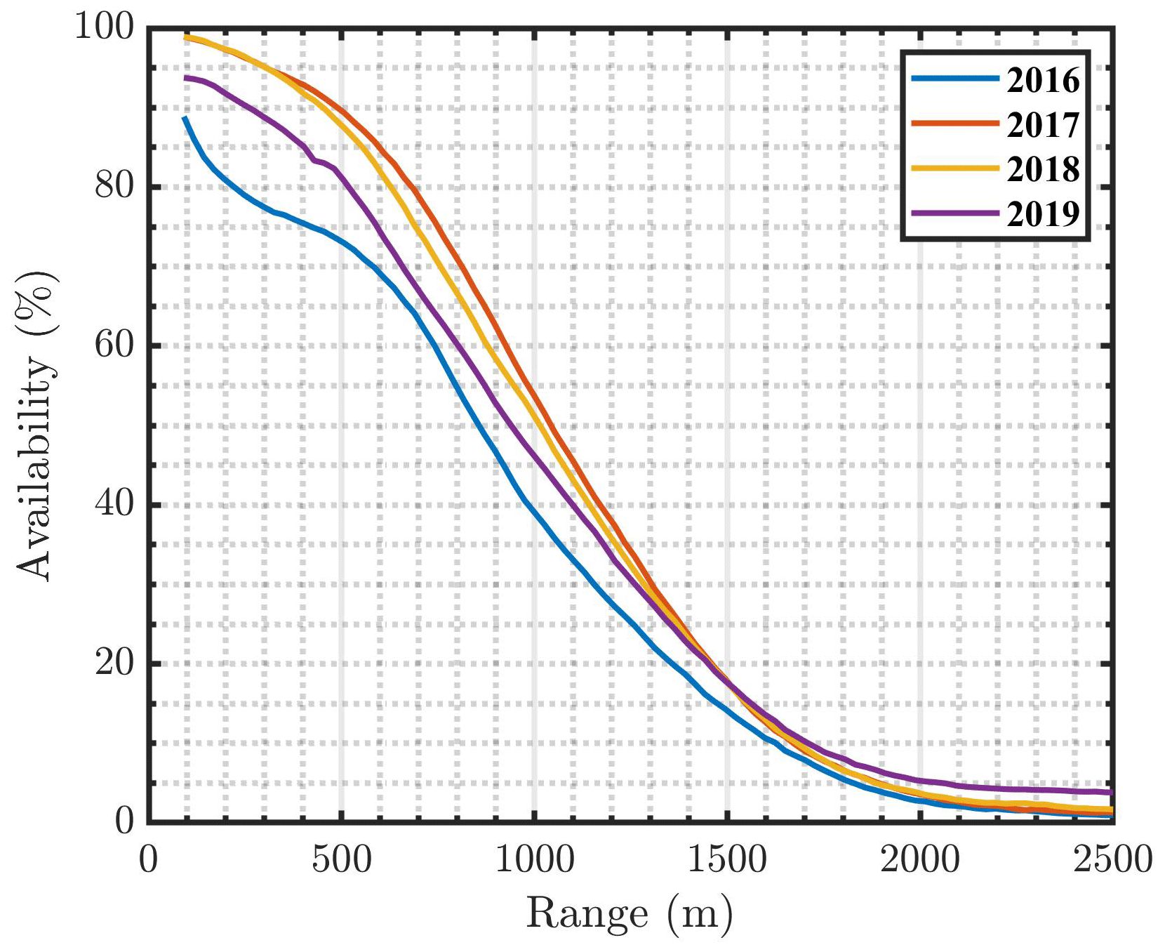
Figure A2 ARM SGP C1 Doppler lidar wind speed profile range availability versus range using processed VAD scans from 2016 to 2019 after SNR filtering (threshold of 1.008 dB).

Appendix B

The RF model develops several regression trees by regrouping the data based on several input features. Figure B1 below shows one of the trees developed by the model used in this article. The leaf nodes are the z_i estimates from radiosondes, and the split nodes represent the surface and lidar data shown in Table 1. MATLAB built-in functions were used for the development of the RF model.

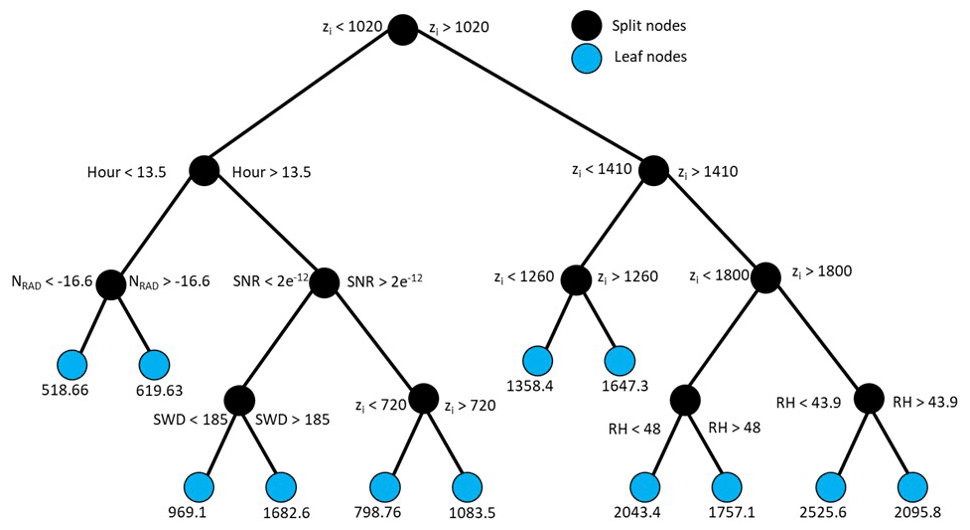
Figure B1 A sample regression tree developed by the RF model. z_i is the Tucker method boundary layer height estimate, SNR is signal-to-noise ratio, NRAD is the normal radiation, RH is relative humidity, SWD is surface wind direction, Hour is hour of the day. The black circles represent the split nodes, and the cyan circles represent the leaf nodes developed for this regression tree (a.k.a. boundary layer height estimates from radiosondes).