the Creative Commons Attribution 4.0 License.
the Creative Commons Attribution 4.0 License.
 | 23 Jun 2021
Assessing sub-grid variability within satellite pixels over urban regions using airborne mapping spectrometer measurements
David P. Edwards
Louisa K. Emmons
Helen M. Worden
Laura M. Judd
Lok N. Lamsal
Jassim A. Al-Saadi
Scott J. Janz
James H. Crawford
Merritt N. Deeter
Gabriele Pfister
Rebecca R. Buchholz
Benjamin Gaubert
Caroline R. Nowlan
Sub-grid variability (SGV) in atmospheric trace gases within satellite pixels is a key issue in satellite design and interpretation and validation of retrieval products. However, characterizing this variability is challenging due to the lack of independent high-resolution measurements. Here we use tropospheric NO2 vertical column (VC) measurements from the Geostationary Trace gas and Aerosol Sensor Optimization (GeoTASO) airborne instrument with a spatial resolution of about 250 m×250 m to quantify the normalized SGV (i.e., the standard deviation of the sub-grid GeoTASO values within the sampled satellite pixel divided by the mean of the sub-grid GeoTASO values within the same satellite pixel) for different hypothetical satellite pixel sizes over urban regions. We use the GeoTASO measurements over the Seoul Metropolitan Area (SMA) and Busan region of South Korea during the 2016 KORUS-AQ field campaign and over the Los Angeles Basin, USA, during the 2017 Student Airborne Research Program (SARP) field campaign. We find that the normalized SGV of NO2 VC increases with increasing satellite pixel sizes (from ∼10 % for 0.5 km×0.5 km pixel size to ∼35 % for 25 km×25 km pixel size), and this relationship holds for the three study regions, which are also within the domains of upcoming geostationary satellite air quality missions. We also quantify the temporal variability in the retrieved NO2 VC within the same hypothetical satellite pixels (represented by the difference of retrieved values at two or more different times in a day). For a given satellite pixel size, the temporal variability within the same satellite pixels increases with the sampling time difference over the SMA. For a given small (e.g., ≤4 h) sampling time difference within the same satellite pixels, the temporal variability in the retrieved NO2 VC increases with the increasing spatial resolution over the SMA, Busan region, and the Los Angeles Basin.
The results of this study have implications for future satellite design and retrieval interpretation and validation when comparing pixel data with local observations. In addition, the analyses presented in this study are equally applicable in model evaluation when comparing model grid values to local observations. Results from the Weather Research and Forecasting model coupled with Chemistry (WRF-Chem) model indicate that the normalized satellite SGV of tropospheric NO2 VC calculated in this study could serve as an upper bound to the satellite SGV of other species (e.g., CO and SO2) that share common source(s) with NO2 but have relatively longer lifetime.
- Article
(3579 KB) - Full-text XML
-
Supplement
(3914 KB) - BibTeX
- EndNote


Characterizing sub-grid variability (SGV) of atmospheric chemical constituent fields is important in both satellite retrievals and atmospheric chemical-transport modeling. This is especially the case over urban regions where strong variability and heterogeneity exist. The inability to resolve sub-grid details is one of the fundamental limitations of grid-based models (Qian et al., 2010) and has been studied extensively (e.g., Boersma et al., 2016; Ching et al., 2006; Denby et al., 2011; Pillai et al., 2010; Qian et al., 2010). Pillai et al. (2010) found that the SGV of column-averaged carbon dioxide (CO2) can reach up to 1.2 ppm in global models that have a horizontal resolution of 100 km. This is an order of magnitude larger than sampling errors that include both limitations in instrument precision and uncertainty of unresolved atmospheric CO2 variability within the mixed layer (Gerbig et al., 2003). Denby et al. (2011) suggested that the average European urban background exposure for nitrogen dioxide (NO2) using a model of 50 km resolution is underestimated by ∼44 % due to SGV.
In contrast, much less attention has been paid to the sub-grid variability within satellite pixels (e.g., Broccardo et al., 2018; Judd et al., 2019; Tack et al., 2021). Indeed, some previous studies (e.g., Kim et al., 2016; Song et al., 2018; Zhang et al., 2019; Choi et al., 2020) used satellite retrievals to study SGV in models and calculated representativeness errors of model results with respect to the satellite measurements (e.g., Pillai et al., 2010). Even though satellite retrievals of atmospheric composition often have lower uncertainties than model results, it has not been until recently that the typical spatial resolution of atmospheric composition satellite products has reached scales comparable to regional atmospheric chemistry models (≲10 km).
Quantification of satellite SGV has historically been limited by insufficient spatial coverage of in situ measurements and is a key issue in designing, understanding, validating, and correctly interpreting satellite observations. This is especially important in the satellite instrument development process during which the required measurement precision and retrieval resolution need to be defined in order to meet the mission science goals. In addition, when validating and evaluating relatively coarse-scale satellite retrievals by comparing them with surface in situ observations, SGV introduces high uncertainties on top of the existing uncertainty introduced by imperfect knowledge of the trace gas vertical profiles. Accurate quantification of satellite SGV can therefore facilitate the estimate of sampling uncertainty for satellite product validation and evaluation. Temporal variability within sampled satellite pixels is also an important issue in satellite design, validation, and application. For polar-orbiting satellites, knowledge of temporal variability is necessary to analyze the representativeness of satellite retrievals at specific overpass times. For geostationary Earth orbit (GEO) satellites, developing a measure of the temporal variability in fine-scale spatial structure will be important for assessing coincidence during validation of the new hourly observations. This work is partly motivated by validation requirements and considerations for the upcoming GEO satellite constellation for atmospheric composition that includes the Tropospheric Emissions: Monitoring Pollution (TEMPO) mission over North America (Chance et al., 2013; Zoogman et al., 2017), the Geostationary Environment Monitoring Spectrometer (GEMS) over Asia (Kim et al., 2020), and the Sentinel-4 mission over Europe (Courrèges-Lacoste et al., 2017).
Airborne mapping spectrometer measurements provide dense observations within the several-kilometer footprint of a typical satellite pixel. This feature of airborne mapping spectrometer measurements provides a unique opportunity to estimate satellite SGV in addition to its role in satellite validation. For example, Broccardo et al. (2018) used aircraft measurements of NO2 from an imaging differential optical absorption spectrometer (iDOAS) instrument to study intra-pixel variability in satellite tropospheric NO2 column over South Africa, whilst Judd et al. (2019) evaluated the impact of spatial resolution on tropospheric NO2 column comparisons with in situ observations using the NO2 measurements of the Geostationary Trace gas and Aerosol Sensor Optimization (GeoTASO). GeoTASO is an airborne remote sensing instrument capable of high-spatial-resolution retrieval of ultraviolet–visible (UV–VIS) absorbing species such as NO2 and formaldehyde (HCHO; Nowlan et al., 2018) and sulfur dioxide (SO2; Chong et al., 2020), and it has measurement characteristics similar to the GEMS and TEMPO GEO satellite instruments. The GeoTASO data used here were taken in gapless, grid-like patterns – or “rasters” – over the regions of interest, providing essentially continuous spatial coverage that was repeated during multiple flights up to 4 times a day in some cases. As such, the GeoTASO data (with a spatial resolution of ) provide a preview of the type of sampling that is expected from the GEO satellite sensors, making the data particularly suitable for our study. We focus on the GeoTASO measurements made during the Korea–United States Air Quality (KORUS-AQ) field experiment in 2016 (Crawford et al., 2021). The measurements from KORUS-AQ have been widely used by researchers for various air quality topics, including quantification of emissions and model and satellite evaluation (e.g., Deeter et al., 2019; Huang et al., 2018; Kim et al., 2018; Miyazaki et al., 2019; Spinei et al., 2018; Tang et al., 2018, 2019; Souri et al., 2020; Gaubert et al., 2020). We further compare our findings from KORUS-AQ with flights conducted during the NASA Student Airborne Research Program (SARP) in 2017 over the Los Angeles (LA) Basin to test the general applicability of our findings over a different urban region. The KORUS-AQ mission took place within the GEMS domain, while the SARP in 2017 is within the domain of TEMPO. Given the similarity between the TEMPO and GEMS instruments in terms of spectral ranges, spectral and spatial resolution, and retrieval algorithms (Al-Saadi et al., 2015), such a comparison is reasonable and useful in facilitating the generalization of the results from the study.
We use the tropospheric NO2 vertical column (VC) retrieved by GeoTASO as a tool to assess satellite SGV and temporal variability for different hypothetical satellite pixel sizes over urban regions. Because spatial SGV and temporal variability both vary with satellite pixel size, the two need to be considered together to enhance the accuracy of satellite product analyses. NO2 is an important air pollutant that is primarily generated from anthropogenic sources such as emissions from the energy, transportation, and industry sectors (Hoesly et al., 2018). It is a reactive gas with a typical lifetime of a few hours in the planetary boundary layer (PBL), although it can also be transported over long distance in the form of peroxyacetyl nitrate (PAN) and nitric acid. NO2 is a precursor of tropospheric ozone and secondary aerosols and has a negative impact on human health and the environment (Finlayson-Pitts and Pitts, 1997). The results from this paper's analysis of NO2 also have implications for other air pollutants that share common source(s) with NO2 but that have somewhat longer lifetimes, for example, carbon monoxide (CO) and SO2.
In this study, we apply a satellite pixel random sampling technique and the spatial structure function analysis to GeoTASO data (described in Sect. 2) to quantify the SGV of satellite pixel NO2 VC over three urban regions at a variety of spatial resolutions. We analyze the relationship between satellite pixel size and satellite SGV, and the relationship between satellite pixel size and the temporal variability in NO2 observations (Sect. 3). We then discuss the implications for satellite design, satellite retrieval interpretation, satellite validation and evaluation, and satellite and in situ data comparisons (Sect. 4). Implications for general local observations and grid data comparisons are also discussed. Section 5 presents our conclusions.
In this section, we describe the GeoTASO instrument, campaign flights, and the different analysis techniques used to characterize the satellite pixel SGV. We outline two approaches: satellite pixel random sampling to investigate separately both spatial variability and temporal variability and the construction of spatial structure functions for an alternative measure of spatial variability.
2.1 GeoTASO instrument
In this study, we focus on GeoTASO retrievals of tropospheric NO2 VC. GeoTASO is a hyperspectral instrument (Leitch et al., 2014) that measures nadir backscattered light in the ultraviolet (UV; 290–400 nm) and visible (VIS; 415–695 nm). As one of NASA's airborne UV–VIS mapping instruments, it was designed to support the upcoming GEO satellite missions by acquiring high-temporal- and high-spatial-resolution measurements with dense sampling for optimizing and experimenting with new retrieval algorithms (Leitch et al., 2014; Nowlan et al., 2016; Lamsal et al., 2017; Judd et al., 2019).
NO2 is retrieved from GeoTASO spectra using the differential optical absorption spectroscopy (DOAS) technique. The retrieval methods and level 2 data processing are described in Lamsal et al. (2017) and Souri et al. (2020) for KORUS-AQ and in Judd et al. (2019) for SARP. Although beyond the scope of this work, it is important to recognize that assumptions made in the retrieval process (e.g., assumed vertical distribution of the NO2 profile) could affect the final variability in the retrieved NO2 fields. GeoTASO has a cross-track field of view of 45∘ (±22.5∘ from nadir), and the retrieval pixel size is approximately 250 m×250 m from typical flight altitudes of 24 000–28 000 ft (7.3–8.5 km). The dense sampling of airborne remote sensing measurements such as GeoTASO is a unique feature that provides the opportunity to study the expected spatial and temporal variability within satellite-retrieved NO2 pixels at high resolution. We use cloud-free GeoTASO data in this study. GeoTASO NO2 VC retrievals have been validated with aircraft in situ data and ground-based Pandora spectrometer remote sensing measurements during KORUS-AQ. Validation of GeoTASO NO2 VC retrievals with aircraft in situ data suggested ∼25 % average difference, while agreement with Pandora is better with a difference of ∼10 % on average. Mean difference between Pandora and aircraft in situ data is ∼20 %. These validation results of GeoTASO NO2 VC retrievals are better than that reported by Nowlan et al. (2016). GeoTASO NO2 VC retrievals during 2017 SARP have also been validated with Pandora data (Judd et al., 2019).
2.2 The 2016 KORUS-AQ field campaign
The KORUS-AQ field measurement campaign (Crawford et al., 2021) took place in May–June 2016 to help understand the factors controlling air quality over South Korea. One of the goals of KORUS-AQ was the testing and improvement of remote sensing algorithms in advance of the launches of the GEMS, TEMPO, and Sentinel-4 satellite missions. It is hoped that the high-quality initial data products from the GEO missions will facilitate their rapid uptake in air quality applications after launch (Al-Saadi et al., 2015; Kim et al., 2020). During KORUS-AQ, GeoTASO flew on board the NASA LaRC B200 aircraft. We focus on the data taken over the Seoul Metropolitan Area (SMA) that is highly urbanized and polluted and the greater Busan region that is less urbanized and less polluted than the SMA (Fig. 1). Figure 2 shows the 12 GeoTASO data rasters (i.e., gapless maps) acquired over the SMA. It took ∼4 h to sample the large-area rasters (i.e., May 11 AM, May 17 AM, May 17 PM, and May 28 PM) and ∼2 h to sample small-area rasters (i.e., June 01 PM, June 02 AM, June 05 AM, June 09 AM, and June 09 PM). Figure S1 in the Supplement shows the two GeoTASO rasters acquired over the Busan region.
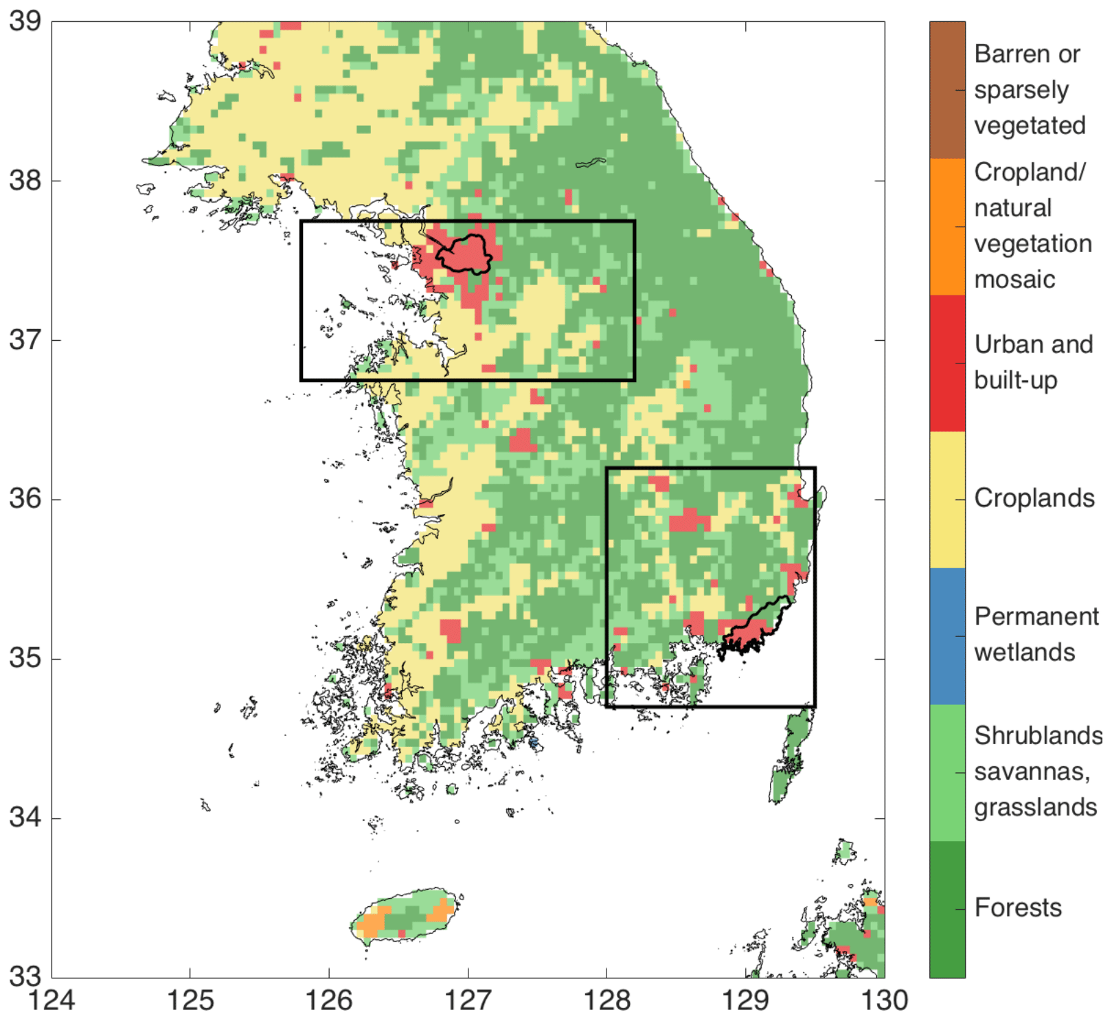
Figure 1Domain of the study over South Korea and the land cover. Boxes indicate location of the SMA (upper left) and the Busan region (lower right) domains. The bold polygons in the two boxes represents the political boundaries (upper left) of Seoul and Busan (lower right). Land cover data are from MODIS Terra and Aqua MCD12C1 L3 product, version V006, annual mean at 0.05∘ resolution; Friedl and Sulla-Menashe et al. (2015).
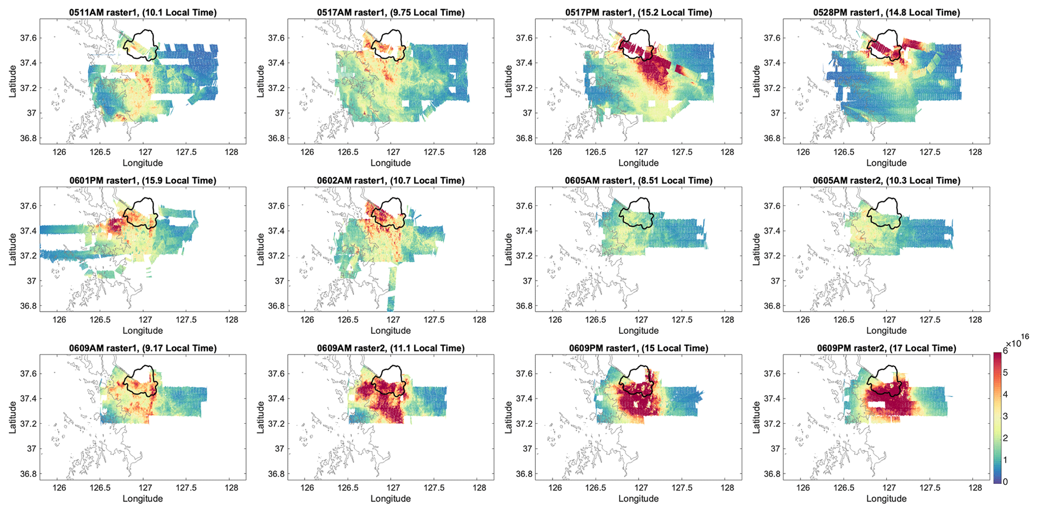
Figure 2GeoTASO data of tropospheric NO2 vertical column (molec. cm−2) measured during KORUS-AQ over the Seoul region. Each panel shows a separate raster. Panel titles show month, day, AM/PM, raster number on that date, and mean time of raster acquisition. There were nine flights sampling rasters over Seoul. The 1 May AM, 17 May AM, 17 May PM, 28 May PM, 1 June PM, and 2 June AM flights each sampled one raster. The 5 June AM, 9 June AM, and 9 June PM flights each sampled two rasters. As a result, there were two flights and two rasters on 17 May, one flight and two rasters on 5 June, and two flights and four rasters on 9 June. The bold polygons in each panel represent the political boundary of Seoul.
2.3 The 2017 SARP field campaign
During the NASA Student Airborne Research Program (SARP) flights in June 2017 (https://airbornescience.nasa.gov/content/Student_Airborne_Research_Program, last access: 7 June 2021), GeoTASO was flown on board the NASA LaRC UC-12B aircraft over the LA Basin (Fig. S2, which also shows the land cover). A detailed description and analysis of these data can be found in Judd et al. (2018, 2019). In this study, we compare our analyses of the KORUS-AQ GeoTASO data with that from SARP over the LA Basin to test the general applicability of our findings.
2.4 Satellite pixel random sampling for spatial variability
The sampling strategy with GeoTASO provides a raster of continuous measurements in a mapped gapless pattern at high spatial resolution (Figs. 2, S1, and S2). This dataset allows us to sample and study the SGV of coarser-spatial-resolution hypothetical satellite pixels sampling the same domain. To mimic satellite observations and quantify the satellite SGV, we randomly sample the GeoTASO data with hypothetical satellite pixels spanning 27 different pixel sizes (0.5 km×0.5 km, 0.75 km×0.75 km, 1 km×1 km, 2 km×2 km, up to 25 km×25 km). Because of the transition to better spatial resolution for the future satellite missions and the coverage limitation in the maximum hypothetical satellite pixel size sampled using the random sampling method, the analysis of SGV only goes up to 25 km×25 km. This sampling process is conducted for each hour of each selected flight over the regions of interest during the KORUS-AQ and SARP campaigns. For every sampled satellite pixel, the mean (MEANpixel) and standard deviation (SDpixel) of the GeoTASO tropospheric NO2 VC data within the pixel are calculated to represent the satellite SGV. Normalized satellite SGV is calculated as the standard deviation of the GeoTASO data within the sampled satellite pixel divided by the mean of the GeoTASO data within the same sampled satellite pixel (SDpixel/MEANpixel).
We use a set of 10 000 hypothetical satellite pixels at each size to include all of the GeoTASO data in the analysis and to cover as many locations as possible. Because the data are located closely in space but may be sampled at slightly different times for the same flight, we separate GeoTASO data into hourly bins for each flight before pixel sampling in order to reduce the impact of temporal variability in the GeoTASO data within a single satellite pixel sample.
As an illustration, we describe the procedure below for the 17 May afternoon flight (Fig. 3) that was conducted from 13:00 to 17:00 local time: (1) the GeoTASO data during this flight were divided into four hourly groups according to the measurement time, i.e., 13:00–14:00, 14:00–15:00, 15:00–16:00, and 16:00–17:00; (2) for each of the 27 hypothetical satellite pixel sizes, we randomly generate 10 000 satellite pixel locations within each hourly group. Therefore, for each hour, we sample 270 000 satellite pixels (27 different satellite pixel sizes and 10 000 samples for each size), and for this example flight, we have a total of up to 1 080 000 possible satellite pixels in each of the four hourly groups. Note that only ∼10 % of these samples are used in the analysis because we discarded a sampled satellite pixel if less than 75 % of its area is covered by GeoTASO data. After applying this 75 % area coverage filter, the actual sample size decreases when the pixel size increases. The number of samples is sufficient as our sensitivity tests indicate that the results do not change by halving the sample size. We also tested other choices of the coverage threshold over the SMA in addition to 75 % (not shown here). The results are similar for small pixels (≲10 km2) as they are more likely to be covered by GeoTASO data regardless of the threshold value. For larger pixels (≳15 km2), the satellite SGV is slightly lower when using 30 % or 50 % as the area coverage threshold because larger pixels act like smaller pixels when only partially covered. The threshold of 75 % was chosen as a trade-off between sample size and representation.
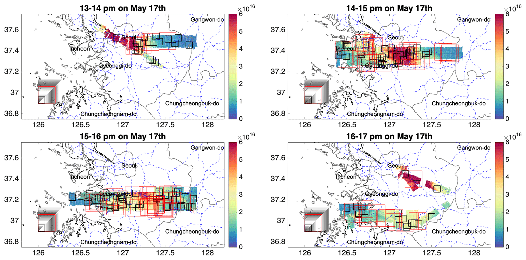
Figure 3Demonstration of the hypothetical satellite pixel random sampling method. Each subplot is 1 h during the 17 May PM flight. For each hour, we randomly sample 10 000 hypothetical satellite pixels at each different pixel size (i.e., 0.5 km×0.5 km, 0.75 km×0.75 km, 1 km×1 km, ) over the GeoTASO data of tropospheric NO2 vertical column (molec. cm−2) every hour. The sampled pixel size (from 0.5 km×0.5 km to 25 km×25 km) are shown in the lower-left corner of each sub-plot. Only 100 samples for pixel size of 7 km×7 km (thick black box) and 100 samples for 18 km×18 km are shown for demonstration purposes. Samples that fail to pass the 75 % coverage threshold are not shown. Coastlines and provincial and metropolitan city boundaries are shown by solid gray lines. Main roads are shown by dashed blue lines (data are from http://www.diva-gis.org/gdata, last access: 7 June 2021).
2.5 Satellite pixel random sampling for temporal variability
We also quantify the temporal variability in the retrieved NO2 VC within the same satellite pixels for different satellite pixel sizes. To calculate temporal variability within a hypothetical satellite pixel, we need GeoTASO data to cover the hypothetical satellite pixel at different times during the day. During the KORUS-AQ and 2017 SARP campaigns, rasters were treated as single units (Judd et al., 2019). Each raster produces a contiguous map of data that we consider as roughly representative of the mid-time of the raster. Unlike the calculation of SGV, which is based on data separated into hourly bins (Sect. 2.4) to reduce the impact of temporal variability in the calculated spatial variability, the satellite pixel random sampling to assess temporal variability is based on rasters and is only conducted for days with multiple rasters. This is to ensure that the sampled hypothetical satellite pixels have multiple values at different times of the day and hence to maximize the sample size.
To assess temporal variability within the hypothetical satellite pixels, we randomly select 50 000 pixel locations for each of the 27 hypothetical satellite pixel sizes and use this same set of pixel locations to sample the GeoTASO data for each raster across all flights for a given day. This process is repeated for all days with multiple rasters, and the 75 % of area coverage threshold is also applied. When there are two or more raster values of MEANpixel for a given pixel location separated by time Dt, the temporal mean difference (TeMD) within the satellite pixel is calculated as follows:
This procedure is repeated for each satellite pixel size.
2.6 Spatial structure function
Structure functions have been applied to in situ measurements and model-generated tropospheric trace gases to analyze their spatial and temporal variability in previous studies (Harris et al., 2001). The spatial structure function (SSF) (Fishman et al., 2011; Follette-Cook et al., 2015) is an alternative measure to the satellite pixel random sampling described above for quantifying spatial variability, and in this work, we apply the SSF to GeoTASO data to assist our analysis of satellite SGV. The main difference between the two measures is that the SSF is based on individual GeoTASO data points, while the results from satellite pixel random sampling are based on sampled satellite pixels. The locations of the GeoTASO pixel centers are used to calculate the distances. The SSF as defined here follows Follette-Cook et al. (2015):
where NO2, VC is tropospheric NO2 VC, and calculates the average of the absolute value of NO2, VC differences across all data pairs (measured in the same hourly bin) that are separated by a distance D. To calculate SSF, the first step is the same as the first step of the satellite pixel random sampling: we group GeoTASO data hourly for each flight to reduce the impact of temporal variability in the GeoTASO data, and we only pair each GeoTASO data point with all the other GeoTASO data in the same hourly bin. More details on structure functions can be found in Follette-Cook et al. (2015).
2.7 WRF-Chem simulation
To briefly demonstrate the application of this technique on model evaluation and other species, we show results of a WRF-Chem simulation (Weather Research and Forecasting model coupled with Chemistry) with a resolution of 3 km×3 km over the SMA in Sect. 4. The simulation used NCEP GDAS/FNL 0.25 Degree Global Tropospheric Analyses and Forecast Grids (National Centers for Environmental Prediction/National Weather Service/NOAA/U.S. Department of Commerce, 2015) as initial and boundary conditions, and the model meteorological fields above the PBL were nudged 6-hourly. KORUS version 3 anthropogenic emissions and FINN version 1.5 fire emissions (Wiedinmyer et al., 2011) were used.
In this section, we discuss the results for SGV over the different regions considered. Results are presented for the hypothetical satellite pixel random sampling for spatial variability and temporal variability and for the spatial structure function analysis. We note that the three regions analyzed in this study are urban. Although we expect the results here to be generally applicable over urban regions, we have not tested the approach over cleaner background areas that are characterized by much less heterogeneity.
3.1 Sub-grid variability (SGV) within satellite pixels
The SMA, the Busan region, and the LA Basin have different levels of pollution – the average values of the GeoTASO NO2 VC data over the SMA, the Busan region, and the LA Basin are 2.3×10¹⁶, 1.1×10¹⁶, and 1.3×10¹⁶ molec. cm−2, respectively. Over the three regions, the mean values (MEANpixel) and standard deviation (SDpixel) of the hypothetical satellite pixels sampled over GeoTASO NO2 VC data are different (Fig. S3). This is consistent with previous studies suggesting SGV can vary regionally (Judd et al., 2019; Broccardo et al., 2018). However, we find that the normalized satellite SGV (calculated as the ratio of SDpixel to MEANpixel for a sampled pixel) is similar over each of the areas regardless of the absolute level of pollution as represented by MEANpixel (Fig. 4). Over the SMA (Fig. 4a), the mean normalized satellite SGV of tropospheric NO2 VC increases smoothly from ∼10 % for the pixel size of 0.5 km×0.5 km to ∼35 % for the pixel size of 25 km×25 km. The interquartile variation in the satellite SGV also increases with satellite pixel sizes. The patterns of the sampled satellite pixels over the Busan region (Fig. 4b) and LA Basin (Fig. 4c) are also found to be similar to those over the SMA. Furthermore, Figs. S4 and S5 show that even the normalized SGV of individual flights over the three domains generally follows the same pattern, except in the case of the 9 June PM flight.
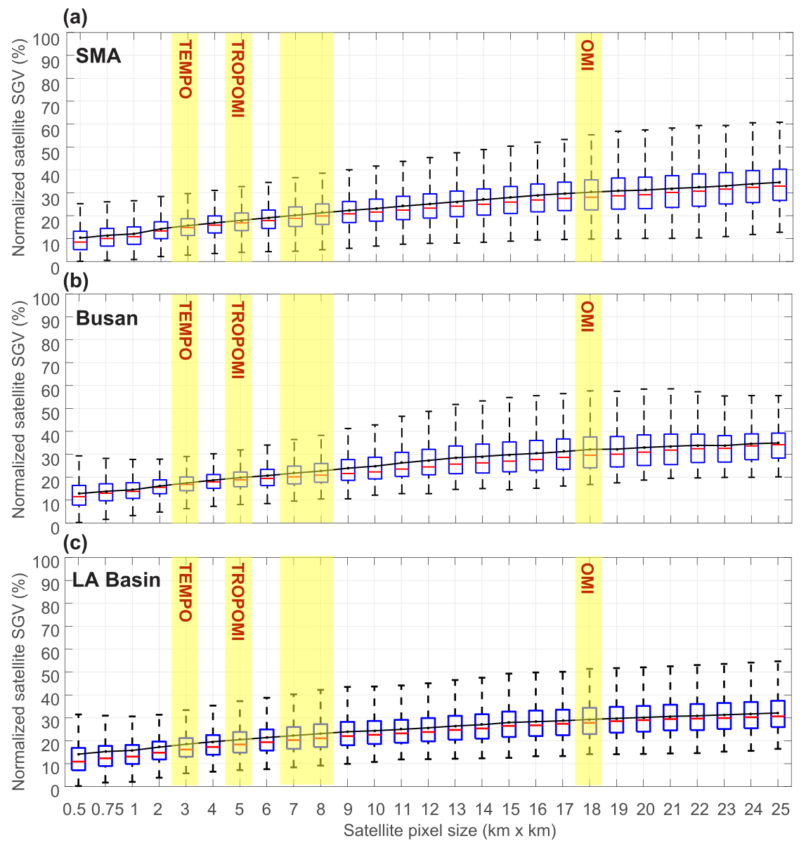
Figure 4Boxplot (with medians represented by red bars, interquartile ranges between 25th and 75th percentiles represented by blue boxes, and the most extreme data points not considered outliers represented by whiskers) for the normalized satellite sub-grid variability (SGV) over the Seoul Metropolitan Area (a), the Busan region (b), and Los Angeles Basin (c). Normalized satellite SGV is calculated as the standard deviation of the GeoTASO data within the sampled satellite pixel divided by the mean of the GeoTASO data within the sampled satellite pixel. The black lines represent the mean of the normalized satellite SGV at a given size. The resolutions of TEMPO, TROPOMI, GEMS, and OMI are highlighted by the yellow shading in the figure.
We also compare normalized satellite SGV for different levels of pollution regardless of their regions (Fig. S6). The normalized satellite SGV for the less polluted pixels (MEANpixel being lower than the average value of all pixels, i.e., 2×10¹⁶ molec. cm−2) also shows an overall similar pattern as for the more polluted pixels (MEANpixel being higher than the average value of all pixels). We notice that at small pixel sizes, less polluted pixels have higher normalized satellite SGV, possibly contributed by relatively higher GeoTASO retrieval noise at lower pollution levels.
We show the normalized SGV for individual rasters over the SMA (Fig. 5) to indicate the uncertainty range of the normalized SGV shown in Fig. 4. The spread of SGV across different individual rasters represents the uncertainties of using the averaged normalized SGV for a specific case. Note that the variation in normalized SGV with pixel size for individual rasters generally follows the same pattern (i.e., increases with satellite pixel size), especially when the pixel size is small (). The normalized SGV increases from ∼10 % to ∼25 %, with the uncertainty range consistently being ±5 % when the pixel size is smaller than 10 km×10 km. When the pixel size is larger than 10 km×10 km, the uncertainty range broadens with pixel sizes from ±5 % (10 km×10 km) to ±15 % (25 km×25 km). This means that when the satellite pixel size is large, using the mean normalized SGV in Fig. 4 to represent specific cases may lead to higher uncertainties. Below the resolution of 10 km×10 km, SGV can be characterized by the mean value with relatively lower uncertainty (±5 %) and hence high confidence, even with large diurnal or day-to-day variations. The spatial resolutions of TEMPO, GEMS, Sentinel-4, and TROPOMI (TROPOspheric Monitoring Instrument; Veefkind et al., 2012; Griffin et al., 2019; van Geffen et al., 2019) are within this range, while the resolution of the Ozone Monitoring Instrument (OMI; Levelt et al., 2006, 2018) is not. This means that applying this study (e.g., Fig. 4) to OMI for a specific case study (e.g., a specific day) requires extra caution.

Figure 5Average of the normalized satellite sub-grid variability (SGV) sampled individually from the 12 rasters (represented by the colored lines) and sampled from all the 12 rasters together (represented by the black line) over the Seoul Metropolitan Area during KORUS-AQ. Normalized satellite SGV is calculated by the standard deviation of the GeoTASO data within the sampled satellite pixel divided by the mean of the GeoTASO data within the sampled satellite pixel.
The GeoTASO data located closely in space may be sampled at slightly different times for the same flight. To explore the impact of temporal variability on this SGV analysis, we performed two sensitivity tests. The typical time period for a complete flight is ∼4 h. In the first test, we sampled GeoTASO data with hypothetical satellite pixels grouped by each complete flight rather than grouping the data by each hour (i.e., hourly bins). The resulting patterns and relationships are similar to those derived from grouping data into hourly bins, except that the normalized satellite SGV increases ∼5 % for small pixels due to temporal variability (Fig. S7a). In the second test, we sampled GeoTASO data with hypothetical satellite pixels grouped by each raster. The results are still similar to those derived from grouping data into hourly bins (Fig. 4), except that the normalized satellite SGV increases ∼1 % for small pixels due to the inclusion of temporal variability (Fig. S7b). This is because sampling by raster includes lower temporal variability than sampling by flight but higher temporal variability than sampling by hourly bins.
The three regions investigated in this work have different levels of urbanization and air pollution (Figs. 1 and S2). PBL conditions are also different in the morning and afternoon (Fig. S8). The similarity of the relationships between the satellite pixel size and the normalized satellite SGV over these different regions (Fig. 4) suggests that this relationship may be generalizable to NO2 VC over urban regions with different levels of urbanization and air pollution and different PBL conditions. Moreover, Figs. 4 and 5 point to the possibility of developing a generalized look-up table for the expected normalized satellite SGV for NO2 VC over urban regions at different satellite pixel sizes, especially for small pixel sizes (e.g., TEMPO, GEMS, and TROPOMI). This would be useful in satellite design, satellite retrieval evaluation and interpretation, and satellite and in situ data comparisons. For example, the satellite pixel size of tropospheric NO2 VC retrievals from GEMS, TEMPO, TROPOMI, and OMI are highlighted in Fig. 4. Following Judd et al. (2019), we choose 3 km×3 km, 5 km×5 km, 7 km×8 km, and 18 km×18 km pixels to represent the expected area of the satellite pixels for TEMPO (2.1 km×4.4 km), TROPOMI (3.5 km×7 km), GEMS (7 km×8 km), and OMI (18 km×18 km), respectively. The expected normalized satellite SGV for TEMPO, TROPOMI, GEMS, and OMI are 15 %–20 %, ∼20 %, 20 %–25 %, and ∼30 %, respectively. Taking the TEMPO example, this implies that the satellite SGV could potentially lead to uncertainties of 15 %–20 % in a validation exercise comparing a satellite retrieval with local measurements of NO2 VC, from a Pandora spectrometer for example, that may be unrepresentative of the wider pixel area.
3.2 Temporal variability (TeMD) within the same satellite pixels
In addition to satellite spatial SGV, we also analyze the temporal variability (i.e., TeMD) within the same hypothetical satellite pixels. Figure 6 shows TeMD of satellite-retrieved tropospheric NO2 VC over the SMA as a function of hypothetical satellite pixel size and the separation time (Dt) between flight rasters as described in Sect. 2.5. The results for 27 satellite pixel sizes analyzed are shown by different colors, while results for selected satellite pixel sizes are highlighted by thicker lines. For all the pixel sizes, TeMD increases monotonically with the time difference Dt between two sampled raster values within the same pixel. The TeMD of tropospheric NO2 VC is around 0.75×10¹⁶ molec. cm−2 for a Dt of 2 h over the SMA for all the sampled satellite pixel sizes and increases to molec. cm−2 for Dt of 8 h. This indicates that, along with improvements in the satellite retrieval spatial resolution with smaller pixels, improving the satellite retrieval temporal resolution with higher frequency measurements is also an effective way to enhance capability in resolving variabilities in NO2.
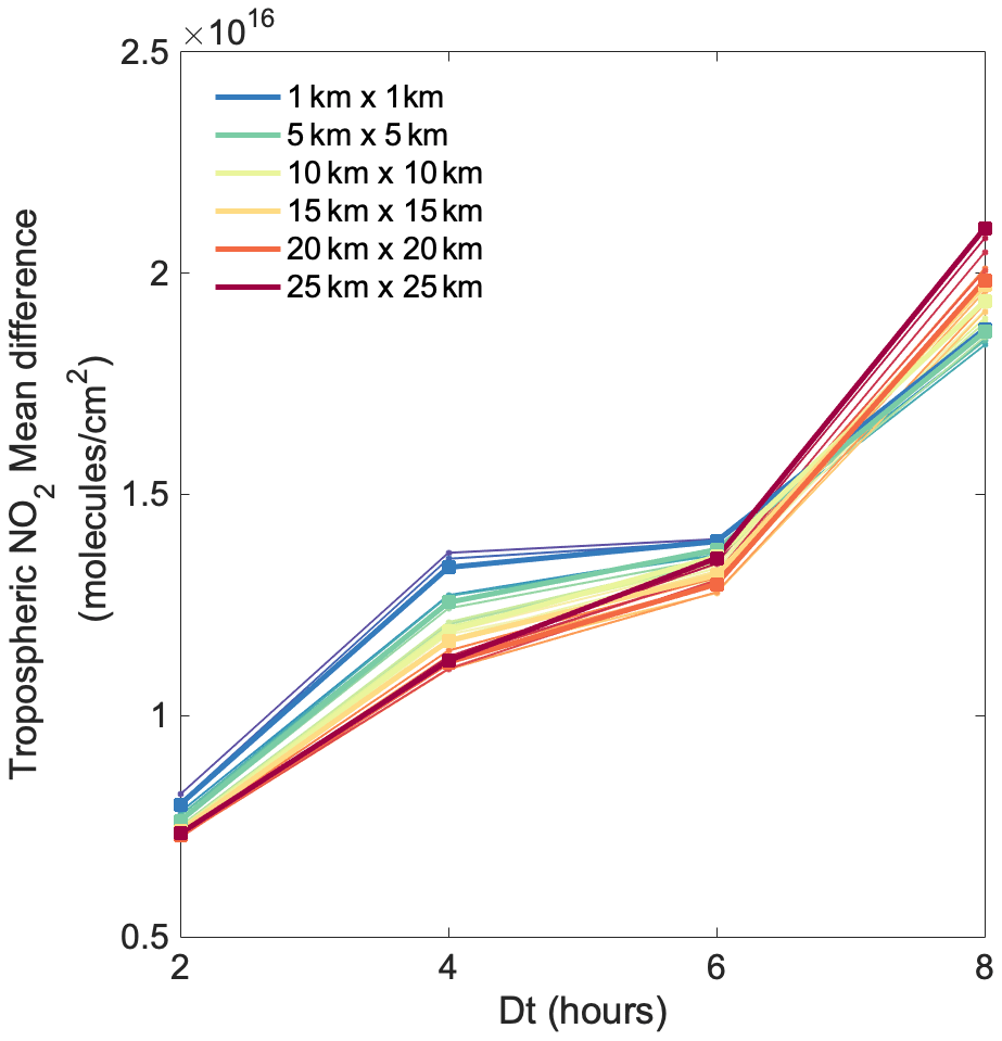
Figure 6Temporal mean differences (TeMDs) of hypothetical satellite pixels (molec. cm−2) over the Seoul Metropolitan Area as a function of time difference (Dt). Results for each pixel size are color coded, with selected sizes shown with thicker lines for reference. See also text for details.
To investigate the TeMD shown in Fig. 6 we consider the particular factors driving NO2 variability over the SMA. NO2 has a relatively short lifetime (∼ a few hours) and a strong diurnal cycle due to emission activities, chemistry, and changing photolysis rate (Fishman et al., 2011; Follette-Cook et al., 2015). The diurnal cycle of the PBL may also play a large role because horizontal dispersion occurs as the PBL thickens during the day. Early in the morning, the PBL is low (∼1400 m during 09:00–11:00 in the SMA during KORUS-AQ), and strong source locations are evident such as traffic on major highways. As the day progresses, the PBL height increases (∼1800 m during 15:00–17:00; Fig. S8) due to enhanced convection, which further induces a stronger horizontal divergence at the top of the convective cell that allows for greater horizontal dispersion to take place along with the divergence. By early afternoon, emissions from all the major sources in the central region have mixed together to form a wide area of high pollution over the urban center with strong gradients of decreasing NO2 out to the surrounding areas. In addition, changing wind conditions (speed and direction; Fig. S9) during the day can also lead to a shift in pollution patterns and result in different pollution conditions for the same pixel at different times of the day. For example, Raster 1 of June 09 AM (09:17) and Raster 2 of June 09 PM (17:00) are used to calculate TeMD for Dt equals 8 h. The differences in wind conditions (Fig. S9) and the pollution patterns (Fig. 2) are large. Judd et al. (2018) point out that the topography over the SMA also plays a role in the ability to mix horizontally as the PBL grows. Therefore, the TeMD can be large between morning and afternoon (i.e., for Dt longer than 6 h).
For a small Dt (2 or 4 h), TeMD increases at higher spatial resolution (i.e., smaller pixel size). This is especially true for short time periods (e.g., 2 and 4 h), which is more important for the GEO satellite measurements. For example, for Dt of 2 h, TeMD for satellite pixels of 1 km×1 km is about 0.80×10¹⁶ molec. cm−2, while TeMD for satellite pixels of 25 km×25 km is about 0.73×10¹⁶ molec. cm−2 (∼9 % lower); when Dt is 4 h, TeMD for satellite pixels of 1 km×1 km is about 1.3×10¹⁶ molec. cm−2, while TeMD for satellite pixels of 25 km×25 km is about 1.1×10¹⁶ molec. cm−2 (∼15 % lower). This indicates that when decreasing pixel size, the temporal variability in the retrieved values will increase even though the normalized satellite spatial SGV decreases. This is expected because averaging over a larger region with high small-scale spatial variability smooths out temporal variability and therefore produces smaller hourly differences. Our finding here is consistent with that of Fishman et al. (2011).
As the time difference Dt increases, the temporal variability TeMD increases for all pixel sizes. However, the TeMD is now greater at large pixel size which is in contrast to the higher TeMD at small pixel size for shorter Dt. This is a result of the pollution pattern that develops over the SMA during the day (9 June) as described above. The higher TeMD reflects the fact that many of the large pixels now span the strong NO2 gradient between the urban and surrounding area resulting in a much higher spatial variability than earlier in the day at a spatial scale not captured with the smaller pixels. As a caution, we note that TeMD for 8 h is determined by only the difference between Raster 1 of June 09 AM and Raster 2 of June 09 PM (Fig. 2) and that the regional coverage for Raster 2 of June 09 PM is different from the coverage of the other PM rasters. Therefore, the relationship of TeMD and spatial resolution for a large Dt (e.g., 6 or 8 h) over the SMA requires further study.
GeoTASO data over the Busan region is limited. Given the fewer flights, we are not able to show how TeMD changes with Dt over the Busan region in this study. However, we are able to show the relationship between TeMD and satellite pixel sizes. During KORUS-AQ, there were only two rasters sampled over Busan with a Dt of 2 h (Fig. S10). For this Dt of 2 h, TeMD increases slightly at higher satellite retrieval spatial resolution (smaller pixel size). More data over the Busan region would help significantly for this analysis. For the LA Basin GeoTASO data, sampled hypothetical satellite pixels show TeMD increases at higher spatial resolution for the available Dt equal to 4 and 8 h (Fig. S11). However, TeMD is fairly constant at these two time differences, which is different to what was observed over the SMA (Fig. 6). We note that with only 2 flight days of flight data, the GeoTASO data over LA is also limited, which may be the main driver of the difference. Besides the limited data, one possible reason is the different wind fields over the two regions. As mentioned previously, Raster 1 of June 09 AM and Raster 2 of June 09 PM are used to calculate TeMD for Dt equals 8 h over the SMA. The differences in wind direction (Fig. S9) for the two rasters are large (almost opposite in some cases). However, over LA, the differences in wind direction (Fig. S12) for the two rasters (rasters 1 and 3 for the June 27 flight) are relatively small compared to the differences over the SMA. Despite the limited sample sizes, TeMD increases when increasing the satellite retrieval spatial resolution over both the Busan region and the LA Basin, which is consistent with the relationships over the SMA for a small Dt.
3.3 Results from spatial structure function (SSF)
In this section, we show the analysis of SSF over the SMA (Fig. 7) as a complement to our analysis in Sect. 3.1. As mentioned before, SSF and SGV are different measures of spatial variability and are not directly comparable. This is because SSF is calculated based on differences between a single GeoTASO measurement and all the other GeoTASO measurements on the map, while SGV is derived based on variation among all the GeoTASO measurements within a hypothetical satellite pixel unit. SSF measures the averaged spatial difference at a given distance, while SGV directly quantifies the expected spatial variability within a satellite pixel at a given size. As both SSF and SGV are related to spatial variability, we include SSF in this study as an extension to SGV.
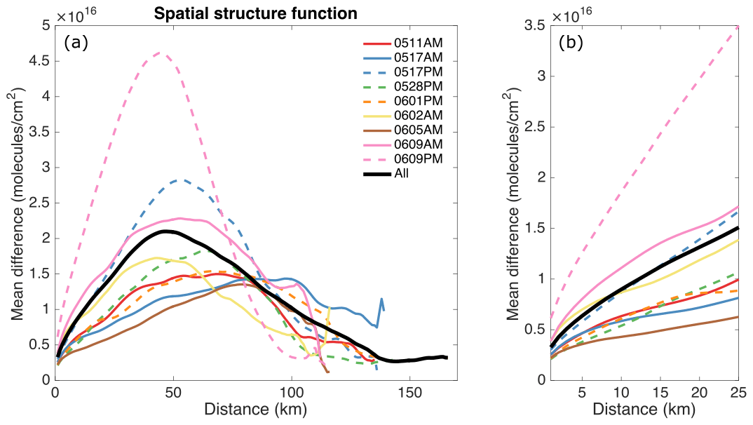
Figure 7(a) Spatial structure function (SSF) for GeoTASO data of tropospheric NO2 vertical column (molec. cm−2) over the Seoul Metropolitan Area (SMA) during KORUS-AQ and (b) the zoom-in version of panel (a) for a distance range of 1–25 km. The SSF calculates the average of the absolute value of NO2, VC differences (i.e., mean difference; y axis) across all data pairs (measured in the same hourly bin) that are separated by different distances (x axis). The SSF based on GeoTASO data measured during morning flights are solid colored lines while the SSF based on GeoTASO data measured during afternoon flights are dashed colored lines. The SSF based on all the data is the solid black line.
Figure 7a shows that the SSF in the SMA initially increases with the distance between data points, peaks at around 40–60 km during most flights, and then decreases with distance between 60 and 140 km. The number of paired GeoTASO data points when the distance is larger than 100 km is relatively small (Fig. S13); therefore conclusions beyond this distance are not included in this analysis. The increases in SSF for distances in the range of 1–25 km (Fig. 7b) are consistent with the relationship between pixel sizes and the normalized satellite SGV shown in Fig. 4. For example, over the 1–25 km range, Fig. 4a shows the median increases from around 8 % to around 28 %, an increase by a factor of 3.5, and the black line in Fig. 7 shows an approximately similar factor (from 0.33×10¹⁶ molec. cm−2 for 1 km to 1.5×10¹⁶ molec. cm−2 for 25 km). This increase in SSF between 1–25 km is also seen over the Busan region and the LA Basin (Fig. S14). We also notice that SSF shows a relatively strong dependence on the particular GeoTASO flight, while SGV is less sensitive, especially for small pixel sizes.
The shapes of the SSF are generally consistent with previous studies for modeled or in situ observations of NO2 (Fishman et al., 2011; Follette-Cook et al., 2015). Previous studies also suggest that different aircraft campaigns may share the common shape of SSF but different magnitudes, which is strongly related to the fraction of polluted samples versus samples of background air in the campaign (Crawford et al., 2009; Fishman et al., 2011). Differences in the shape and size of particular cities also contribute to the differences in the SSF. For example, at a certain distance SSF may compare polluted areas within the same urban region, while over a different smaller city, the comparison at the same distance reveals the gradient between the polluted city and cleaner surrounding background air, thus resulting in different peak values. Valin et al. (2011) found that the maximum in OH feedback in a NOx−OH steady-state relationship corresponds to a NO2 e-folding decay length of 54 km in 5 m s−1 winds. This may partially explain the peak between 40 and 60 km in SSF. As shown in Figs. 2 and S7, the overall spatial variability over the SMA is higher in the afternoon. Over the SMA, the SSF in the morning is generally smaller than in the afternoon, indicating higher spatial variability in tropospheric NO2 VC in the afternoon (see also Judd et al., 2018). As described in Sect. 2.6, SSF is calculated based on hourly binned data. However, the overall shapes of SSF (Fig. S15) calculated on a raster basis are similar to SSF calculated on an hourly basis (Fig. 7).
Previous studies (Fishman et al., 2011; Follette-Cook et al., 2015) used SSF values at a particular distance to indicate the satellite precision requirement at a corresponding resolution in order to resolve spatial structure over the pixel scale. For GEMS, the expected spatial differences over the scale of its pixel for the SMA and Busan regions are and molec. cm−2, respectively, taking the SSF values at 5 km to be representative. For TEMPO, the spatial difference is molec. cm−2 over LA Basin taking the SSF value at 3 km. Assuming the NO2 measurement precision requirement to be 1×10¹⁵ molec. cm−2 for both TEMPO and GEMS (Chance et al., 2013; Kim et al., 2020), the expected spatial differences over the three regions are considerably higher than the precision requirement and should be easily characterized by both the GEMS and TEMPO missions.
The relationship between satellite pixel sizes and the normalized satellite SGV is fairly robust over the three different urban regions studied here, and Fig. 4 points to the possibility of developing a generalized look-up table if more data were available in other urban regions. We note that the GeoTASO data used in this study were sampled during spring and summer. In our future study, we will include more GeoTASO data in the analysis to test the applicability of the look-up table approach under different seasonal conditions and sources. A generalized relationship between satellite pixel sizes and the temporal variability (Fig. 6) is not as evident as the relationship between satellite pixel sizes and the normalized satellite SGV due to limited data. However, it is still useful for satellite observations over the SMA, which is in the GEMS domain and should be helpful in satellite retrieval interpretation.
Previous studies recognized the challenges in satellite validation and evaluation for NO2 retrievals due to satellite SGV and representativeness error of in situ measurements (e.g., Nowlan et al., 2016, 2018; Judd et al., 2019; Pinardi et al., 2020; Tack et al., 2021). The gapless airborne mapping datasets of GeoTASO with sufficient spatiotemporal resolution are a promising way to address the issue of satellite SGV and representativeness errors in satellite validation and evaluation (e.g., Nowlan et al., 2016, 2018; Judd et al., 2019).
Challenges due to SGV also have implications for other trace gas column measurements. For example, in Tang et al. (2020), satellite SGV and representativeness errors of in situ measurements introduced uncertainties in the validation of CO retrievals from the MOPITT (Measurement Of Pollution In The Troposphere) satellite instrument. Normalized SGV of the GeoTASO tropospheric NO2 VC might serve as an upper bound to the SGV of CO, SO2, and other species that share common source(s) with NO2 but with relatively longer lifetimes than NO2, even if their spatial distributions have different patterns (e.g., Chong et al., 2020). For example, at the resolution of 22 km×22 km (resolution of MOPITT CO retrievals), the expected normalized satellite SGV of tropospheric NO2 VC is ∼30 %. Therefore, we might expect the normalized satellite SGV for tropospheric CO VC to be lower than this value.
To demonstrate this idea, we use the WRF-Chem regional model as an intermediary step. At the model resolution, if the SGV of the WRF-Chem model and GeoTASO NO2 VC agree reasonably well, then the model can be used to predict the SGV of other species that are chemically constrained with NO2 at the model and coarser resolutions. This is shown in Fig. 8 which illustrates how SGV varies with satellite pixel size for NO2 VC, CO VC, SO2 VC, and HCHO VC calculated from a WRF-Chem simulation. The modeled NO2, CO, SO2, and HCHO concentrations are converted to VC and are filtered to match the rasters of GeoTASO measurements (Fig. S16). As expected, SGV of modeled NO2 VC is higher than SGV of modeled CO VC, SO2 VC, and HCHO VC. We also notice that SGV for modeled NO2 VC, CO VC, SO2 VC, and HCHO VC increases with pixel size, which is similar to that for GeoTASO measurements. The SGV for GeoTASO NO2 shown in this figure (black lines) is calculated based on GeoTASO data that are regridded to the WRF-Chem grid (3 km×3 km), making it slightly different from that in Fig. 4. We note that the modeled NO2 SGV is greater than that calculated from the GeoTASO data, indicating that further work is required to reconcile difference due to model descriptions of emissions, chemistry, and transport. Ideally, dense GeoTASO-type measurements of CO and other species would allow for a more comprehensive assessment of this approach.
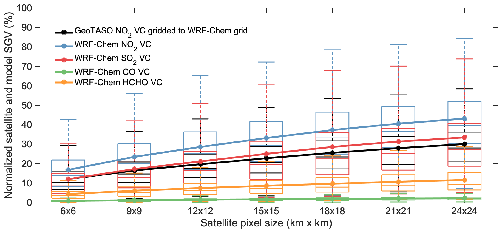
Figure 8Boxplot of hypothetical normalized satellite SGV of NO2 vertical column (VC), SO2 VC, CO VC, and formaldehyde (HCHO) VC derived from the WRF-Chem simulation with a resolution of 3 km×3 km (colored lines) and GeoTASO NO2 VC that gridded to the WRF-Chem grid (black lines) over the Seoul Metropolitan Area. Medians are represented by red bars, interquartile ranges between 25th and 75th percentiles by blue boxes, and the most extreme data points not considered outliers by whiskers. The modeled NO2, CO, SO2, and HCHO are filtered to match the rasters of GeoTASO measurements.
This study is also relevant to model comparison and evaluation with in situ observations. Whenever in situ observations are compared to grid data (e.g., comparisons between satellite retrievals and in situ observations, comparisons between grid-based model and in situ observations, and in data assimilation), SGV will introduce uncertainties that need to be quantified to better interpret and understand the comparison results. For example, we note that at the resolution of 14 km×14 km (a typical resolution for the forward-looking Multi-Scale Infrastructure for Chemistry and Aerosols Version 0; MUSICA-V0, https://www2.acom.ucar.edu/sections/multi-scale-chemistry-modeling-musica, last access: 7 June 2021; Pfister et al., 2020), Fig. 8 shows that the expected normalized SGV of tropospheric NO2 VC is ∼ 25 %–30 %. This suggests that when comparing model simulations at coarser resolution with local observations of tropospheric NO2 VC, a larger normalized SGV than this ∼ 25 %–30 % might be expected. If comparing for a specific vertical layer instead of vertical column, an even larger normalized SGV may occur.
For data assimilation and inverse modeling application (e.g., top-down emission estimations from satellite observations), it is essential to accurately characterize the observation error covariance matrix R (Janjić et al., 2018). The first component of R is the instrument error covariance matrix due to instrument noise and retrieval uncertainty in the case of trace gas satellite data. The second component is the representation error covariance matrix, arising from fundamental differences of the atmospheric sampling typically when assimilating a local point measurement into a grid-based model (Boersma et al., 2016). The observation error covariance due to representativeness error is difficult to define but can be parameterized when calculating super observations by inflating the observation error variances (Boersma et al., 2016) and quantified by a posteriori diagnostics estimation (Gaubert et al., 2014). Knowledge of the fine-scale model sub-grid variability is therefore essential to verify those assumptions and inform error statistics for application to chemical data assimilation studies. Our results suggest large potential improvements in emission estimates when assimilating high-spatial-resolution TROPOMI and GEO satellite data with SGV of ∼ 10 %–20 % (Fig. 4), compared to OMI data with SGV of ∼30 % (Fig. 4), in line with the existing literature for NO2 (e.g., Valin et al., 2011). We have also shown that significant temporal variability in NO2 is expected at higher spatial resolutions. This observed signal will open new avenues for space-based monitoring of atmospheric chemistry and will reduce errors of inverse estimates of fluxes.
Satellite SGV is a key issue in interpreting satellite retrieval results. Quantifying studies have been lacking due to limited observations at high spatial and temporal resolution. In this study, we have quantified likely GEO satellite SGV by using GeoTASO measurements of tropospheric NO2 VC over the urbanized and polluted Seoul Metropolitan Area (SMA) and the less-polluted Busan region during KORUS-AQ and the Los Angeles (LA) Basin during the 2017 SARP campaigns. The main findings of this work are the following:
-
The normalized satellite SGV increases with pixel size based on random sampling of hourly GeoTASO data, from ∼10 % (±5 % for specific cases such as an individual day/time of day) for a pixel size of 0.5 km×0.5 km to ∼35 % (±10 % for specific cases such as an individual day/time of day) for the pixel size of 25 km×25 km. This conclusion holds for all of the three urban regions in this study despite their different levels of urbanization and pollution and for the time of day being morning or afternoon.
-
Due to its relatively shorter atmospheric lifetime, normalized satellite SGV of tropospheric NO2 VC could serve as an upper bound to satellite SGV of CO, SO2, and other species that share common source(s) with NO2. This conclusion is supported by high-resolution WRF-Chem simulations.
-
The temporal variability (TeMD) increases with sampling time differences (Dt) over the SMA. TeMD ranges from molec. cm−2 at Dt of 2 h to molec. cm−2 (about 3 times higher) at Dt of 8 h. TeMD is caused by temporal variation in emission activities, photolysis, and meteorology throughout the day. Improving the satellite retrieval temporal resolution is an effective way to enhance the capability of satellite products in resolving temporal variability in NO2.
-
Temporal variability (TeMD) increases as pixel size decreases in the SMA when the time difference is less than 4 h. Analysis confidence at greater time differences would require more flight datasets with longer time separations during the day. For example, when Dt is 2 h, TeMD for satellite pixels with the size of 25 km×25 km is about 9 % lower compared to TeMD for satellite pixels with the size of 1 km×1 km. Thus, ideally, temporal resolution should be increased along with any increase in spatial resolution in order to enhance the representativeness of satellite products.
-
The spatial structure function (SSF) at first increases with the distance between points, peaking at around 40–60 km during most flight days, before decreasing at greater distances. This is generally consistent with previous studies.
-
SSF analyses suggest that GEMS will encounter NO2 VC pixel-scale spatial differences of and molec. cm−2 over the SMA and Busan regions, respectively. TEMPO will encounter NO2 VC spatial differences at its pixel scale of molec. cm−2 over the LA Basin. These differences should be easily resolved by the instruments at the stated measurement precision requirement of 1×10¹⁵ molec. cm−2.
-
These findings are relevant to future satellite design and satellite retrieval interpretation, especially now with the deployment of the high-resolution GEO air quality satellite constellation, GEMS, TEMPO, and Sentinel-4. This study also has implication for satellite product validation and evaluation, satellite and in situ data comparisons, and more general point-grid data comparisons. These share similar issues of sub-grid variability and the need for the quantification of representativeness error.
We note that this study has some uncertainties and limitations. (1) The variability at a resolution finer than 250 m×250 m (i.e., GeoTASO's resolution) may introduce uncertainties to the analysis here, although this is beyond the scope of this study. (2) Even though a large number of GeoTASO retrievals have been analyzed in this study, we would still benefit from more GeoTASO flights with a broader spatiotemporal coverage. More GeoTASO-type data over the Busan region and LA Basin will help in testing the consistence in TeMD over different regions. (3) The KORUS-AQ campaign was conducted in Spring (May and June), and the 2017 SARP campaign was also conducted in June. More GeoTASO-type measurements over South Korea during different season(s) would be particularly helpful to understand and generalize the findings in this study. (4) The three regions analyzed in this study are urban regions, and the results are not tested over cleaner background areas that may be characterized by less heterogeneity.
This work demonstrates the value of continued flights of GeoTASO-type instruments for obtaining continuous, high-spatial-resolution data several times a day for assessing SGV. This will be a particularly useful reference in the comparisons of satellite retrievals and in situ measurements that may have representativeness errors.
The KORUS-AQ data are available at https://doi.org/10.5067/Suborbital/KORUSAQ/DATA01 (NASA, 2021) and SARP data are available at https://www-air.larc.nasa.gov/missions/lmos/index.html (last access: 7 June 2021, Janz et al., 2021), respectively.
The supplement related to this article is available online at: https://doi.org/10.5194/amt-14-4639-2021-supplement.
DPE and WT designed the study. WT analyzed the data with help from DPE, LMJ, JAA, and LKE. GP provided WRF-Chem results. CRN, HMW, LNL, SJJ, JHC, MND, BG, and RRB offered valuable discussions and comments in improving the study. WT and DPE prepared the paper with improvements from all the other coauthors.
The authors declare that they have no conflict of interest.
The authors thank the GeoTASO team for providing the GeoTASO measurements. The authors thank the KORUS-AQ and SARP team for the campaign data. We thank the DIAL-HSRL team for the mixing layer height data (available at https://www-air.larc.nasa.gov/cgi-bin/ArcView/korusaq, last access: 7 June 2021). Wenfu Tang was supported by a NCAR Advanced Study Program Postdoctoral Fellowship. The authors thank Ivan Ortega and Sara-Eva Martinez-Alonso for helpful comments on the paper. The National Center for Atmospheric Research (NCAR) is sponsored by the National Science Foundation.
David P. Edwards was partially supported by the TEMPO Science Team under Smithsonian Astrophysical Observatory subcontract SV3-83021.
This paper was edited by Michel Van Roozendael and reviewed by three anonymous referees.
Al-Saadi, J., Carmichael, G., Crawford, J., Emmons, L., Kim, S., Song, C.-K., Chang, L.-S., Lee, G., Kim, J., and Park, R.: NASA Contributions to KORUS-AQ: An International Cooperative Air Quality Field Study in Korea, 32 pp., available at: https://espo.nasa.gov/home/korus-aq/content/KORUS-AQ_Science_Overview_0, (last access: 7 June 2021), 2015.
Boersma, K. F., Vinken, G. C. M., and Eskes, H. J.: Representativeness errors in comparing chemistry transport and chemistry climate models with satellite UV–Vis tropospheric column retrievals, Geosci. Model Dev., 9, 875–898, https://doi.org/10.5194/gmd-9-875-2016, 2016.
Broccardo, S., Heue, K.-P., Walter, D., Meyer, C., Kokhanovsky, A., van der A, R., Piketh, S., Langerman, K., and Platt, U.: Intra-pixel variability in satellite tropospheric NO2 column densities derived from simultaneous space-borne and airborne observations over the South African Highveld, Atmos. Meas. Tech., 11, 2797–2819, https://doi.org/10.5194/amt-11-2797-2018, 2018.
Chance, K., Liu, X., Suleiman, R. M., Flittner, D. E., Al-Saadi, J., and Janz, S. J.: Tropospheric emissions: Monitoring of pollution (TEMPO), Proceedings of SPIE, Vol. 8866, Earth Observin Systems XVIII, 88660D, San Diego, CA USA, 23 September 2013.
Ching, J., Herwehe, J., and Swall, J.: On joint deterministic grid modeling and sub-grid variability conceptual framework for model evaluation, Atmos. Environ., 40, 4935–4945, 2006.
Choi, S., Lamsal, L. N., Follette-Cook, M., Joiner, J., Krotkov, N. A., Swartz, W. H., Pickering, K. E., Loughner, C. P., Appel, W., Pfister, G., Saide, P. E., Cohen, R. C., Weinheimer, A. J., and Herman, J. R.: Assessment of NO2 observations during DISCOVER-AQ and KORUS-AQ field campaigns, Atmos. Meas. Tech., 13, 2523–2546, https://doi.org/10.5194/amt-13-2523-2020, 2020.
Chong, H., Lee, S., Kim, J., Jeong, U., Li, C., Krotkov, N. A., Nowlan, C. R., Al-Saadi, J. A., Janz, S. J., Kowalewski, M. G., Ahn, M.-H., Kang, M., Joiner, J., Haffner, D. P., Hu, L., Castellanos, P., Huey, L. G., Choi, M., Song, C. H., Han, K. M., and Koo, J.-H.: High-resolution mapping of SO2 using airborne observations from the GeoTASO instrument during the KORUS-AQ field study: PCA-based vertical column retrievals, Remote Sens. Environ., 241, 111725, https://doi.org/10.1016/j.rse.2020.111725, 2020.
Courrèges-Lacoste, G. B., Sallusti, M., Bulsa, G., Bagnasco, G., Veihelmann, B., Riedl, S., Smith, D. J., and Maurer, R.: The Copernicus Sentinel 4 mission: a geostationary imaging UVN spectrometer for air quality monitoring, Proceedings Volume 10423, Sensors, Systems, and Next-Generation Satellites XXI, 1042307, https://doi.org/10.1117/12.2282158, 2017.
Crawford, J. H.: Assessing scales of variability for constituents relevant to future geostationary satellite observations and models of air quality, AGU Fall Meeting Abstracts, Vol. 2009, A53A-0237, 2009.
Crawford, J. H., Ahn, J.-Y., Al-Saadi, J., Chang, L., Emmons, L. K., Kim, J., Lee, G., Park, J.-H., Park, R., Woo, J. H., Lefer, B. L., Lee, M., Lee, T., Kim, S., Min, K.-E., Yum, S. S., Szykman, J. J., Jordan, C. E., Simpson, I. J., Fried, A., Cho, S., and Kim, Y. P.: The Korea–United States Air Quality (KORUS-AQ) field study, Elementa: Science of the Anthropocene, 9, 00163, https://doi.org/10.1525/elementa.2020.00163, 2021.
Deeter, M. N., Edwards, D. P., Francis, G. L., Gille, J. C., Mao, D., Martínez-Alonso, S., Worden, H. M., Ziskin, D., and Andreae, M. O.: Radiance-based retrieval bias mitigation for the MOPITT instrument: the version 8 product, Atmos. Meas. Tech., 12, 4561–4580, https://doi.org/10.5194/amt-12-4561-2019, 2019.
Denby, B., Cassiani, M., de Smet, P., de Leeuw, F., and Horálek, J.: Sub-grid variability and its impact on European wide air quality exposure assessment, Atmos. Environ., 45, 4220–4229, 2011.
Finlayson-Pitts, B. J. and Pitts Jr., J. N.: Tropospheric air pollution: Ozone, airborne toxics, polycyclic aromatic hydrocarbons, and particles, Science, 276, 1045–1052, 1997.
Fishman, J., Silverman, M. L., Crawford, J. H., and Creilson, J. K.: A study of regional-scale variability of in situ and model-generated tropospheric trace gases: Insights into observational requirements for a satellite in geostationary orbit, Atmos. Environ., 45, 4682–4694, 2011.
Follette-Cook, M., Pickering, K., Crawford, J., Duncan, B., Loughner, C., Diskin, G., Fried, A., and Weinheimer, A.: Spatial and temporal variability of trace gas columns derived from WRF/Chem regional model output: Planning for geostationary observations of atmospheric composition, Atmos. Environ., 118, 28–44, https://doi.org/10.1016/j.atmosenv.2015.07.024, 2015.
Friedl, M. and Sulla-Menashe, D.: MCD12C1 MODIS/Terra+Aqua Land Cover Type Yearly L3 Global 0.05Deg CMG V006, NASA EOSDIS Land Processes DAAC [data set], https://doi.org/10.5067/MODIS/MCD12C1.006, 2015.
Gaubert, B., Coman, A., Foret, G., Meleux, F., Ung, A., Rouil, L., Ionescu, A., Candau, Y., and Beekmann, M.: Regional scale ozone data assimilation using an ensemble Kalman filter and the CHIMERE chemical transport model, Geosci. Model Dev., 7, 283–302, https://doi.org/10.5194/gmd-7-283-2014, 2014.
Gaubert, B., Emmons, L. K., Raeder, K., Tilmes, S., Miyazaki, K., Arellano Jr., A. F., Elguindi, N., Granier, C., Tang, W., Barré, J., Worden, H. M., Buchholz, R. R., Edwards, D. P., Franke, P., Anderson, J. L., Saunois, M., Schroeder, J., Woo, J.-H., Simpson, I. J., Blake, D. R., Meinardi, S., Wennberg, P. O., Crounse, J., Teng, A., Kim, M., Dickerson, R. R., He, H., Ren, X., Pusede, S. E., and Diskin, G. S.: Correcting model biases of CO in East Asia: impact on oxidant distributions during KORUS-AQ, Atmos. Chem. Phys., 20, 14617–14647, https://doi.org/10.5194/acp-20-14617-2020, 2020.
Gerbig, C., Lin, J. C., Wofsy, S. C., Daube, B. C., Andrews, A. E., Stephens, B. B., Bakwin, P. S., and Grainger, C. A.: Toward constraining regional-scale fluxes of CO2 with atmospheric observations over a continent: 1. Observed spatial variability from airborne platforms, J. Geophys. Res.-Atmos., 108, 4756, https://doi.org/10.1029/2002JD003018, 2003.
Griffin, D., Zhao, X., McLinden, C. A., Boersma, F., Bourassa, A., Dammers, E., Degenstein, D., Eskes, H., Fehr, L., Fioletov, V., Hayden, K., Kharol, S. K., Li, S.-M., Makar, P., Martin, R. V., Mihele, C., Mittermeier, R. L., Krotkov, N., Sneep, M., Lamsal, L. N., ter Linden, M., van Geffen, J., Veefkind, P., and Wolde, M.: High-Resolution Mapping of Nitrogen Dioxide with TROPOMI: First Results and Validation Over the Canadian Oil Sands, Geophys. Res. Lett., 46, 1049–1060, https://doi.org/10.1029/2018GL081095, 2019.
Harris, D., Foufoula-Georgiou, E., Droegemeier, K. K., and Levit, J. J.: Multiscale Statistical Properties of a High-Resolution Precipitation Forecast, J. Hydrometeorol., 2, 406–418, 2001.
Hoesly, R. M., Smith, S. J., Feng, L., Klimont, Z., Janssens-Maenhout, G., Pitkanen, T., Seibert, J. J., Vu, L., Andres, R. J., Bolt, R. M., Bond, T. C., Dawidowski, L., Kholod, N., Kurokawa, J.-I., Li, M., Liu, L., Lu, Z., Moura, M. C. P., O'Rourke, P. R., and Zhang, Q.: Historical (1750–2014) anthropogenic emissions of reactive gases and aerosols from the Community Emissions Data System (CEDS), Geosci. Model Dev., 11, 369–408, https://doi.org/10.5194/gmd-11-369-2018, 2018.
Huang, M., Crawford, J. H., Diskin, G. S., Santanello, J. A., Kumar, S. V., Pusede, S. E., Parrington, M., and Carmichael, G. R.: Modeling Regional Pollution Transport Events During KORUS-AQ: Progress and Challenges in Improving Representation of Land-Atmosphere Feedbacks, J. Geophys. Res.-Atmos., 123, 10–732, 2018.
Janjić, T., Bormann, N., Bocquet, M., Carton, J. A., Cohn, S. E., Dance, S. L., Losa, S. N., Nichols, N. K., Potthast, R., Waller, J. A., and Weston, P.: On the representation error in data assimilation, Q. J. Roy. Meteor. Soc., 144, 1257–1278, https://doi.org/10.1002/qj.3130, 2018.
Janz, S., Judd, L., and Kowalewski, M.: Lake Michigan Ozone Study GeoTASO NO2 Vertical Columns, NASA ASDC Lake Michigan Ozone Study Repository [data set], available at: https://www-air.larc.nasa.gov/missions/lmos/index.html, last access: 7 June 2021.
Judd, L. M., Al-Saadi, J. A., Valin, L. C., Pierce, R. B., Yang, K., Janz, S. J., Kowalewski, M. G., Szykman, J. J., Tiefengraber, M., and Mueller, M.: The Dawn of Geostationary Air Quality Monitoring: Case Studies From Seoul and Los Angeles, Front. Environ. Sci., 6, 85, https://doi.org/10.3389/fenvs.2018.00085, 2018.
Judd, L. M., Al-Saadi, J. A., Janz, S. J., Kowalewski, M. G., Pierce, R. B., Szykman, J. J., Valin, L. C., Swap, R., Cede, A., Mueller, M., Tiefengraber, M., Abuhassan, N., and Williams, D.: Evaluating the impact of spatial resolution on tropospheric NO2 column comparisons within urban areas using high-resolution airborne data, Atmos. Meas. Tech., 12, 6091–6111, https://doi.org/10.5194/amt-12-6091-2019, 2019.
Kim, H., Zhang, Q., and Heo, J.: Influence of intense secondary aerosol formation and long-range transport on aerosol chemistry and properties in the Seoul Metropolitan Area during spring time: results from KORUS-AQ, Atmos. Chem. Phys., 18, 7149–7168, https://doi.org/10.5194/acp-18-7149-2018, 2018.
Kim, H. C., Lee, P., Judd, L., Pan, L., and Lefer, B.: OMI NO2 column densities over North American urban cities: the effect of satellite footprint resolution, Geosci. Model Dev., 9, 1111–1123, https://doi.org/10.5194/gmd-9-1111-2016, 2016.
Kim, J., Jeong, U., Ahn, M.-H., Kim, J. H., Park, R. J., Lee, H., Song, C. H., Choi, Y.-S., Lee, K.-H., Yoo, J.-M., Jeong, M.-J., Park, S. K., Lee, K.-M., Song, C.-K., Kim, S.-W., Kim, Y. J., Kim, S.-W., Kim, M., Go, S., Liu, X., Chance, K., Miller, C. C., Al-Saadi, J., Veihelmann, B., Bhartia, P. K., Torres, O., Abad, G. G., Haffner, D. P., Ko, D. H., Lee, S. H., Woo, J.-H., Chong, H., Park, S. S., Nicks, D., Choi, W. J., Moon, K.-J., Cho, A., Yoon, J., Kim, S.-K., Hong, H., Lee, K., Lee, H., Lee, S., Choi, M., Veefkind, P., Levelt, P. F., Edwards, D. P., Kang, M., Eo, M., Bak, J., Baek, K., Kwon, H.-A., Yang, J., Park, J., Han, K. M., Kim, B.-R., Shin, H.-W., Choi, H., Lee, E., Chong, J., Cha, Y., Koo, J.-H., Irie, H., Hayashida, S., Kasai, Y., Kanaya, Y., Liu, C., Lin, J., Crawford, J. H., Carmichael, G. R., Newchurch, M. J., Lefer, B. L., Herman, J. R., Swap, R. J., Lau, A. K. H., Kurosu, T. P., Jaross, G., Ahlers, B., Dobber, M., McElroy, C. T., and Choi, Y.: New era of air quality monitoring from space, Geostationary Environment Monitoring Spectrometer (GEMS), B. Am. Meteorol. Soc., 101, E1–E22, https://doi.org/10.1175/BAMS-D-18-0013.1, 2020.
Lamsal, L. N., Janz, S., Krotkov, N., Pickering, K. E., Spurr, R. J. D., Kowalewski, M., Loughner, C. P., Crawford, J., Swartz, W. H., and Herman, J. R.: High-resolution NO2 observations from the Airborne Compact Atmospheric Mapper: Retrieval and validation, J. Geophys. Res., 122, 1953–1970, https://doi.org/10.1002/2016JD025483, 2017.
Leitch, J. W., Delker, T., Good, W., Ruppert, L., Murcray, F., Chance, K., Liu, X., Nowlan, C., Janz, S. J., Krotkov, N. A., Pickering, K. E., Kowalewski, M., and Wang, J.: The GeoTASO airborne spectrometer project, Earth Observing Systems XIX, 17–21 August 2014, San Diego, California, United States, Proc. SPIE, 9218, 92181H-9, https://doi.org/10.1117/12.2063763, 2014.
Levelt, P. F., Oord, G. H. J. van den, Dobber, M. R., Malkki, A., Visser, H., Vries, J. de, Stammes, P., Lundell, J. O. V., and Saari, H.: The ozone monitoring instrument, IEEE T. Geosci. Remote, 44, 1093–1101, https://doi.org/10.1109/TGRS.2006.872333, 2006.
Levelt, P. F., Joiner, J., Tamminen, J., Veefkind, J. P., Bhartia, P. K., Stein Zweers, D. C., Duncan, B. N., Streets, D. G., Eskes, H., van der A, R., McLinden, C., Fioletov, V., Carn, S., de Laat, J., DeLand, M., Marchenko, S., McPeters, R., Ziemke, J., Fu, D., Liu, X., Pickering, K., Apituley, A., González Abad, G., Arola, A., Boersma, F., Chan Miller, C., Chance, K., de Graaf, M., Hakkarainen, J., Hassinen, S., Ialongo, I., Kleipool, Q., Krotkov, N., Li, C., Lamsal, L., Newman, P., Nowlan, C., Suleiman, R., Tilstra, L. G., Torres, O., Wang, H., and Wargan, K.: The Ozone Monitoring Instrument: overview of 14 years in space, Atmos. Chem. Phys., 18, 5699–5745, https://doi.org/10.5194/acp-18-5699-2018, 2018.
Miyazaki, K., Sekiya, T., Fu, D., Bowman, K., Kulawik, S., Sudo, K., Walker, T., Kanaya, Y., Takigawa, M., Ogochi, K., Eskes, H., Boersma, K. F., Thompson, A. M., Gaubert, B., Barre, J., and Emmons, L. K.: Balance of Emission and Dynamical Controls on Ozone During the Korea-United States Air Quality Campaign From Multiconstituent Satellite Data Assimilation, J. Geophys. Res.-Atmos., 124, 387–413, 2019.
NASA: KORUS-AQ – An International Cooperative Air Quality Field Study in Korea, NASA Langley Research Center Airborne Science Data for Atmospheric Composition, KORUS-AQ data archive [data set], https://doi.org/10.5067/Suborbital/KORUSAQ/DATA01, 2021.
National Centers for Environmental Prediction/National Weather Service/NOAA/U.S. Department of Commerce: NCEP GDAS/FNL 0.25 Degree Global Tropospheric Analyses and Forecast Grids, Research Data Archive at the National Center for Atmospheric Research, Computational and Information Systems Laboratory [data set], https://doi.org/10.5065/D65Q4T4Z, 2015 (updated daily).
Nowlan, C. R., Liu, X., Leitch, J. W., Chance, K., González Abad, G., Liu, C., Zoogman, P., Cole, J., Delker, T., Good, W., Murcray, F., Ruppert, L., Soo, D., Follette-Cook, M. B., Janz, S. J., Kowalewski, M. G., Loughner, C. P., Pickering, K. E., Herman, J. R., Beaver, M. R., Long, R. W., Szykman, J. J., Judd, L. M., Kelley, P., Luke, W. T., Ren, X., and Al-Saadi, J. A.: Nitrogen dioxide observations from the Geostationary Trace gas and Aerosol Sensor Optimization (GeoTASO) airborne instrument: Retrieval algorithm and measurements during DISCOVER-AQ Texas 2013, Atmos. Meas. Tech., 9, 2647–2668, https://doi.org/10.5194/amt-9-2647-2016, 2016.
Nowlan, C. R., Liu, X., Janz, S. J., Kowalewski, M. G., Chance, K., Follette-Cook, M. B., Fried, A., González Abad, G., Herman, J. R., Judd, L. M., Kwon, H.-A., Loughner, C. P., Pickering, K. E., Richter, D., Spinei, E., Walega, J., Weibring, P., and Weinheimer, A. J.: Nitrogen dioxide and formaldehyde measurements from the GEOstationary Coastal and Air Pollution Events (GEO-CAPE) Airborne Simulator over Houston, Texas, Atmos. Meas. Tech., 11, 5941–5964, https://doi.org/10.5194/amt-11-5941-2018, 2018.
Pfister, G. G., Eastham, S. D., Arellano, A. F., Aumont, B., Barsanti, K. C., Barth, M. C., Conley, A., Davis, N. A., Emmons, L. K., Fast, J. D., Fiore, A. M., Gaubert, B., Goldhaber, S., Granier, C., Grell, G. A., Guevara, M., Henze, D. K., Hodzic, A., Liu, X., Marsh, D. R., Orlando, J. J., Plane, J. M. C., Polvani, L. M., Rosenlof, K. H., Steiner, A. L., Jacob, D. J., and Brasseur, G. P.: The Multi-Scale Infrastructure for Chemistry and Aerosols (MUSICA), B. Am. Meteorol. Soc., 101, 1743–1760, 2020.
Pillai, D., Gerbig, C., Marshall, J., Ahmadov, R., Kretschmer, R., Koch, T., and Karstens, U.: High resolution modeling of CO22 over Europe: implications for representation errors of satellite retrievals, Atmos. Chem. Phys., 10, 83–94, https://doi.org/10.5194/acp-10-83-2010, 2010.
Pinardi, G., Van Roozendael, M., Hendrick, F., Theys, N., Abuhassan, N., Bais, A., Boersma, F., Cede, A., Chong, J., Donner, S., Drosoglou, T., Dzhola, A., Eskes, H., Frieß, U., Granville, J., Herman, J. R., Holla, R., Hovila, J., Irie, H., Kanaya, Y., Karagkiozidis, D., Kouremeti, N., Lambert, J.-C., Ma, J., Peters, E., Piters, A., Postylyakov, O., Richter, A., Remmers, J., Takashima, H., Tiefengraber, M., Valks, P., Vlemmix, T., Wagner, T., and Wittrock, F.: Validation of tropospheric NO2 column measurements of GOME-2A and OMI using MAX-DOAS and direct sun network observations, Atmos. Meas. Tech., 13, 6141–6174, https://doi.org/10.5194/amt-13-6141-2020, 2020.
Qian, Y., Gustafson Jr., W. I., and Fast, J. D.: An investigation of the sub-grid variability of trace gases and aerosols for global climate modeling, Atmos. Chem. Phys., 10, 6917–6946, https://doi.org/10.5194/acp-10-6917-2010, 2010.
Song, H., Zhang, Z., Ma, P.-L., Ghan, S., and Wang, M.: The importance of considering sub-grid cloud variability when using satellite observations to evaluate the cloud and precipitation simulations in climate models, Geosci. Model Dev., 11, 3147–3158, https://doi.org/10.5194/gmd-11-3147-2018, 2018.
Spinei, E., Whitehill, A., Fried, A., Tiefengraber, M., Knepp, T. N., Herndon, S., Herman, J. R., Müller, M., Abuhassan, N., Cede, A., Richter, D., Walega, J., Crawford, J., Szykman, J., Valin, L., Williams, D. J., Long, R., Swap, R. J., Lee, Y., Nowak, N., and Poche, B.: The first evaluation of formaldehyde column observations by improved Pandora spectrometers during the KORUS-AQ field study, Atmos. Meas. Tech., 11, 4943–4961, https://doi.org/10.5194/amt-11-4943-2018, 2018.
Souri, A. H., Nowlan, C. R., Wolfe, G. M., Lamsal, L. N., Chan Miller, C. E., Abad, G. G., Janz, S. J., Fried, A., Blake, D. R., Weinheimer, A. J., Diskin, G. S., Liu, X., and Chance, K.: Revisiting the effectiveness of ratios for inferring ozone sensitivity to its precursors using high resolution airborne remote sensing observations in a high ozone episode during the KORUS-AQ campaign, Atmos. Environ., 224, 117341, https://doi.org/10.1016/j.atmosenv.2020.117341, 2020.
Tack, F., Merlaud, A., Iordache, M.-D., Pinardi, G., Dimitropoulou, E., Eskes, H., Bomans, B., Veefkind, P., and Van Roozendael, M.: Assessment of the TROPOMI tropospheric NO2 product based on airborne APEX observations, Atmos. Meas. Tech., 14, 615–646, https://doi.org/10.5194/amt-14-615-2021, 2021.
Tang, W., Arellano, A. F., DiGangi, J. P., Choi, Y., Diskin, G. S., Agustí-Panareda, A., Parrington, M., Massart, S., Gaubert, B., Lee, Y., Kim, D., Jung, J., Hong, J., Hong, J.-W., Kanaya, Y., Lee, M., Stauffer, R. M., Thompson, A. M., Flynn, J. H., and Woo, J.-H.: Evaluating high-resolution forecasts of atmospheric CO and CO2 from a global prediction system during KORUS-AQ field campaign, Atmos. Chem. Phys., 18, 11007–11030, https://doi.org/10.5194/acp-18-11007-2018, 2018.
Tang, W., Emmons, L. K., Arellano Jr., A. F., Gaubert, B., Knote, C., Tilmes, S., Buchholz, R. R., Pfister, G. G., Diskin, G. S., Blake, D. R., Blake, N. J., Meinardi, S., DiGangi, J. P., Choi, Y., Woo, J.-H., He, C., Schroeder, J. R., Suh, I., Lee, H.-J., Jo, H.-Y., Kanaya, Y., Jung, J., Lee, Y., and Kim, D.: Source contributions to carbon monoxide concentrations during KORUS-AQ based on CAM-chem model applications, J. Geophys. Res.-Atmos., 124, 1–27, https://doi.org/10.1029/2018jd029151, 2019.
Tang, W., Worden, H. M., Deeter, M. N., Edwards, D. P., Emmons, L. K., Martínez-Alonso, S., Gaubert, B., Buchholz, R. R., Diskin, G. S., Dickerson, R. R., Ren, X., He, H., and Kondo, Y.: Assessing Measurements of Pollution in the Troposphere (MOPITT) carbon monoxide retrievals over urban versus non-urban regions, Atmos. Meas. Tech., 13, 1337–1356, https://doi.org/10.5194/amt-13-1337-2020, 2020.
Valin, L. C., Russell, A. R., Hudman, R. C., and Cohen, R. C.: Effects of model resolution on the interpretation of satellite NO2 observations, Atmos. Chem. Phys., 11, 11647–11655, https://doi.org/10.5194/acp-11-11647-2011, 2011.
van Geffen, J., Boersma, K. F., Eskes, H., Sneep, M., ter Linden, M., Zara, M., and Veefkind, J. P.: S5P TROPOMI NO2 slant column retrieval: method, stability, uncertainties and comparisons with OMI, Atmos. Meas. Tech., 13, 1315–1335, https://doi.org/10.5194/amt-13-1315-2020, 2020.
Veefkind, J. P., Aben, I., McMullan, K., Förster, H., de Vries, J., Otter, G., Claas, J., Eskes, H. J., de Haan, J. F., Kleipool, Q., van Weele, M., Hasekamp, O., Hoogeveen, R., Landgraf, J., Snel, R., Tol, P., Ingmann, P., Voors, R., Kruizinga, B., Vink, R., Visser, H., and Levelt, P. F.: TROPOMI on the ESA Sentinel-5 Precursor: A GMES mission for global observations of the atmospheric composition for climate, air quality and ozone layer applications, Remote Sens. Environ., 120, 70–83, https://doi.org/10.1016/j.rse.2011.09.027, 2012.
Wiedinmyer, C., Akagi, S. K., Yokelson, R. J., Emmons, L. K., Al-Saadi, J. A., Orlando, J. J., and Soja, A. J.: The Fire INventory from NCAR (FINN): a high resolution global model to estimate the emissions from open burning, Geosci. Model Dev., 4, 625–641, https://doi.org/10.5194/gmd-4-625-2011, 2011.
Zhang, Z., Song, H., Ma, P.-L., Larson, V. E., Wang, M., Dong, X., and Wang, J.: Subgrid variations of the cloud water and droplet number concentration over the tropical ocean: satellite observations and implications for warm rain simulations in climate models, Atmos. Chem. Phys., 19, 1077–1096, https://doi.org/10.5194/acp-19-1077-2019, 2019.
Zoogman, P., Liu, X., Suleiman, R., Pennington, W., Flittner, D., Al-Saadi, J., Hilton, B., Nicks, D., Newchurch, M., Carr, J., Janz, S., Andraschko, M., Arola, A., Baker, B., Canova, B., Miller, C. C., Cohen, R., Davis, J., Dussault, M., Edwards, D., Fishman, J., Ghulam, A., Abad, G. G., Grutter, M., Herman, J., Houck, J., Jacob, D., Joiner, J., Kerridge, B., Kim, J., Krotkov, N., Lamsal, L., Li, C., Lindfors, A., Martin, R., McElroy, C., McLinden, C., Natraj, V., Neil, D., Nowlan, C., O'Sullivan, E., Palmer, P., Pierce, R., Pippin, M., Saiz-Lopez, A., Spurr, R., Szykman, J., Torres, O., Veefkind, J., Veihelmann, B., Wang, H., Wang, J., and Chance, K.: Tropospheric emissions: Monitoring of pollution (TEMPO), J. Quant. Spectrosc. Ra., 186, 17–39, https://doi.org/10.1016/j.jqsrt.2016.05.008, 2017.