the Creative Commons Attribution 4.0 License.
the Creative Commons Attribution 4.0 License.
 | 08 Jul 2021
Estimating mean molecular weight, carbon number, and OM∕OC with mid-infrared spectroscopy in organic particulate matter samples from a monitoring network
Amir Yazdani
Ann M. Dillner
Satoshi Takahama
Organic matter (OM) is a major constituent of fine particulate matter, which contributes significantly to degradation of visibility and radiative forcing, and causes adverse health effects. However, due to its sheer compositional complexity, OM is difficult to characterize in its entirety. Mid-infrared spectroscopy has previously proven useful in the study of OM by providing extensive information about functional group composition with high mass recovery. Herein, we introduce a new method for obtaining additional characteristics such as mean carbon number and molecular weight of these complex organic mixtures using the aliphatic C−H absorbance profile in the mid-infrared spectrum. We apply this technique to spectra acquired non-destructively from Teflon filters used for fine particulate matter quantification at selected sites of the Inter-agency Monitoring of PROtected Visual Environments (IMPROVE) network. Since carbon number and molecular weight are important characteristics used by recent conceptual models to describe evolution in OM composition, this technique can provide semi-quantitative, observational constraints of these variables at the scale of the network. For this task, multivariate statistical models are trained on calibration spectra prepared from atmospherically relevant laboratory standards and are applied to ambient samples. Then, the physical basis linking the absorbance profile of this relatively narrow region in the mid-infrared spectrum to the molecular structure is investigated using a classification approach. The multivariate statistical models predict mean carbon number and molecular weight that are consistent with previous values of organic-mass-to-organic-carbon () ratios estimated for the network using different approaches. The results are also consistent with temporal and spatial variations in these quantities associated with aging processes and different source classes (anthropogenic, biogenic, and burning sources). For instance, the statistical models estimate higher mean carbon number for urban samples and smaller, more fragmented molecules for samples in which substantial aging is anticipated.
- Article
(6718 KB) - Full-text XML
-
Supplement
(484 KB) - BibTeX
- EndNote


1.1 Organic aerosols and measurement methods
Organic matter (OM) is known to be an important constituent of fine particulate matter (PM). It is estimated to constitute 20 %–50 % of the total fine PM at midlatitudes and up to 90 % in tropical forests (Kanakidou et al., 2005). This organic fraction contributes significantly to aerosol-related phenomena such as visibility and climate change, through radiative forcing and affecting cloud formation, and causes adverse health effects (Shiraiwa et al., 2017b; Hallquist et al., 2009). Such effects underscore the importance of better quantification of organic fraction in particulate matter, which is a complex mixture of a multitude of compounds whose compositions, concentrations, and formation mechanisms are not yet completely understood (Turpin et al., 2000).
The determination of organic aerosol composition involves a large range of analytical and computational techniques. Among the widely known techniques are gas chromatography/mass spectrometry (GC/MS), mid-infrared spectroscopy – often referred to as Fourier transform infrared spectroscopy (FT-IR) – and aerosol mass spectrometry (AMS). GC/MS provides molecular speciation information but is limited to a small mass fraction of the organic aerosols as low as 10 % (Hallquist et al., 2009). AMS and FT-IR, however, can be used to analyze most of the organic mass in addition to providing information about either chemical classes or functional groups (Hallquist et al., 2009). AMS is an online technique with a relatively high size and time resolution. Nevertheless, the extensive fragmentation caused by commonly used ionization method in AMS, i.e., electron impact (EI) ionization, makes the identification of original species difficult (Canagaratna et al., 2007; Faber et al., 2017). In recent years, soft ionization methods such as electrospray ionization (ESI), photoionization (PI), and chemical ionization (CI) have been used frequently for predicting physicochemical properties of organic aerosol (OA), e.g., volatility (Li et al., 2016; Xie et al., 2020), phase state, and viscosity (Li et al., 2020; DeRieux et al., 2018; Shiraiwa et al., 2017a), as a function of measured elemental composition and molecular weight. These methods minimize analyte fragmentation, providing better estimates of molar mass of individual molecules but often have other shortcomings such as ionization efficiency, which varies by molecule (Nozière et al., 2015; Iyer et al., 2016; Hermans et al., 2017; Lopez-Hilfiker et al., 2019).
In mid-infrared spectroscopy, the vibrational modes of organic molecules, whose frequencies fall in the range of mid-infrared electromagnetic radiation, are excited. The advantages of mid-infrared spectroscopy over other common techniques of quantifying OM are providing direct information on functional groups, while minimizing sample alteration during the analysis and having low sampling and analytical cost (Ruthenburg et al., 2014). However, this method only provides bulk functional group (FG) information and has uncertainties regarding the absorption coefficient for group frequencies (although this coefficient is roughly similar across different compounds; Hastings et al., 1952). Moreover, interpretation of mid-infrared spectrum is often complicated due to presence of overlapping peaks. In previous studies, different statistical methods were used to connect mid-infrared absorbances to molar abundance of different functional groups, from which OM, OC (organic carbon), and the ratio were calculated with minimal assumptions (Coury and Dillner, 2008; Ruthenburg et al., 2014; Takahama et al., 2016; Boris et al., 2019). These studies showed good agreement between FT-IR measurements and other methods of OM characterization. For example, Boris et al. (2019) showed that OC measured by FT-IR is around 80 % of OC from thermal optical reflectance (TOR) measurements.
In addition to the abundance of organic functional groups, mid-infrared spectroscopy is informative regarding the environment in which organic bonds are vibrating (e.g., degree of hydrogen bonding; Pavia et al., 2008); therefore, it can be used to extract more detailed structural information about OM. This ability of mid-infrared spectroscopy has been investigated to a lesser extent in the context of atmospheric OM. In this work, we used this aspect to investigate two important structural parameters in OM, i.e., mean molecular weight, and mean carbon number. These two parameters are important characteristics used by recent conceptual models and parameterizations to describe evolution in atmospheric OM, in terms of its volatility and phase state (Shiraiwa et al., 2017a; Pankow and Barsanti, 2009; Kroll et al., 2011; Donahue et al., 2011). Moreover, inspecting the spatial and temporal variations of these parameters helps us understand the processes involved in aerosol aging, especially fragmentation (Murphy et al., 2012), and can be useful for identification of the dominant sources (Price et al., 2017; Gentner et al., 2012).
In this paper, the mean molecular weight, carbon number, and ratio of ambient aerosols, which were collected on polytetrafluoroethylene (PTFE) filters at selected Inter-agency Monitoring of PROtected Visual Environments (IMPROVE) sites, were estimated using FT-IR spectroscopy. First, the aliphatic C−H region (2800–3000 cm−1) was extracted from the baseline-corrected spectra of laboratory standards. The C−H spectral bands were then normalized to eliminate abundance information. Then, partial least squares regression (PLSR) was used to develop models on the high-dimensional and collinear spectral data. Thereafter, the derived statistical models were used to estimate the mean properties of ambient samples. Finally, a classification algorithm was applied to the PLSR model estimates to provide a better understanding of how they function.
1.2 Aliphatic C−H absorption and the molecular structure
We have used the aliphatic C−H region (2800–3000 cm−1) in the mid-infrared spectrum to build statistical models for estimating molecular weight and carbon number. This section describes the connection of that region of the spectrum with the molecular structure of organic aerosols and compares the approach used in this work with previous studies.
Recent studies using FT-IR and AMS have shown that the aliphatic C−H is the most abundant functional group in organic aerosols (Russell et al., 2009; Ruthenburg et al., 2014; Zhang et al., 2007), highlighting its importance in OM. This functional group also exhibits characteristics of “good group” frequencies in the mid-infrared stretch region (Mayo et al., 2004). Since the hydrogen atom is much lighter than the carbon atom, most of the displacement during oscillation is related to the hydrogen; thereby, the carbon atom, and consequently its connection to the rest of the molecule, is involved to a much lesser extent in the stretch (Mayo et al., 2004). This phenomenon results in a fairly consistent profile for the C−H absorption band among different molecules containing this functional group and makes it possible to reduce the dimensionality of spectrum to few independent variables describing the band profile (advantageous when constructing statistical models using a limited number of samples). The light hydrogen atom also causes the aliphatic C−H functional group to absorb at a relatively high stretch frequency, making it isolated from most of other absorbing bonds (Mayo et al., 2004) except the broad carboxylic acid O−H stretch, which absorbs in the 2400–3400 cm−1 range and the ammonium N−H stretch (Pavia et al., 2008). These broad absorption profiles can be separated from the narrow aliphatic C−H bands by baseline correction. The unsaturated and aromatic C−H bonds, which absorb at a slightly higher frequency than aliphatic C−H, were not considered in this work. These bonds are not prevalent in atmospheric samples (Russell et al., 2011; Decesari et al., 2000) and their absorption usually falls below the FT-IR detection limit (Russell et al., 2009). The absorption bands attributed to unsaturated and aromatic C−H were not visible in the mid-infrared spectra of atmospheric samples of this study.
The aliphatic C−H (sp3-hybridized) stretching band in the mid-infrared spectrum is composed of four absorption peaks (two doublets) that are attributed to CH2 (methylene) and CH3 (methyl) symmetric and asymmetric stretches (Mayo et al., 2004). Methine (tertiary CH) also absorbs in this region but has a very weak absorption compared to methyl and methylene (Pavia et al., 2008). The profile of these four peaks (characterized by peak frequency, intensity, and width) is affected by the structure of the molecule, inter- and intra-molecular interactions that change electron distribution, and the equilibrium geometry of the molecule (Atkins et al., 2017; Kelly, 2013) as discussed below.
Group vibrational modes in a molecule are not completely decoupled from the rest of the molecule (McHale, 2017). Equation (1) describes a two-body harmonic oscillator model of molecular vibration (from a classical point of view), for which is the fundamental wavenumber at which the bond vibrates, c is the speed of light, K is the spring constant of the chemical bond, mH is mass of hydrogen atom, and mM is the mass of the rest of the molecule (assuming the rest of the molecule is stiff). The reduced mass of the system, μ, increases with increasing the molecular weight (Eq. 1), resulting in a decreased vibrational frequency (wavenumber). There are also effects that change the vibrational frequency through changing the bond strength. For example, the electron-withdrawing effect of neighboring polar groups and ring structure strain elevate the absorption frequency of the oscillator by increasing the equivalent spring constant (Pavia et al., 2008). The Bohlmann effect, in which electron density is transferred from the lone pair of a neighboring nitrogen or oxygen into the C−H anti-bonding orbital, decreases the frequency by weakening the C−H bond (Lii et al., 2004). Hydrogen-bonding interactions and phase state can also affect absorption frequency and intensity of bands corresponding to vibrational modes (Fornaro et al., 2015; Kelly, 2013):
The environment in which the molecules vibrate can affect the absorption peak width through different homogeneous and inhomogeneous broadening mechanisms. Slightly different interaction of molecules in liquids and amorphous solids (to a lesser extent in crystals) is the basis of inhomogeneous broadening (Kelly, 2013). This phenomenon determines the change in peak width due to phase state by changing the level of interaction between the molecules. Hydrogen bonding can also cause inhomogeneous broadening due to enhanced anharmonicity (Thomas et al., 2013). The weak hydrogen bond, which can exists for aliphatic C−H functional group (Desiraju and Steiner, 2001), broadens its absorption band slightly and shifts its absorption frequency.
The peak height ratios in the aliphatic C−H region are also indicators of some structural features of the molecule. For example, the ratio of peak heights of asymmetric CH3 stretching to asymmetric CH2 stretching shows the relative abundance of these groups in the sample (Orthous-Daunay et al., 2013). For straight-chain alkanes and some polymers, this ratio is directly related to the chain length and can be used to estimate the carbon number of a molecule (Lipp, 1986; Mayo et al., 2004). This ratio as well as the tertiary C−H absorption are informative about the degree of branching in the molecule. The ratio of symmetric to asymmetric CH2 peak heights is an indicator of rotational and conformational order in a molecule, and is related to chain length and phase state (Hähner et al., 2005; Corsetti et al., 2017; Orendorff et al., 2002). Price et al. (2017) compared that ratio between mid-infrared spectra of emissions under different engine conditions for ultra-low sulfur diesel (ULSD) and hydrogenation-derived renewable diesel (HDRD) fuels, observed a slightly greater ratio for the ULSD emissions, and suggested this was due to the differences in the carbon number distribution of the two fuel emissions. In addition, some other vibrational bands can affect this region through forming overtones and combination bands (Thomas, 2017).
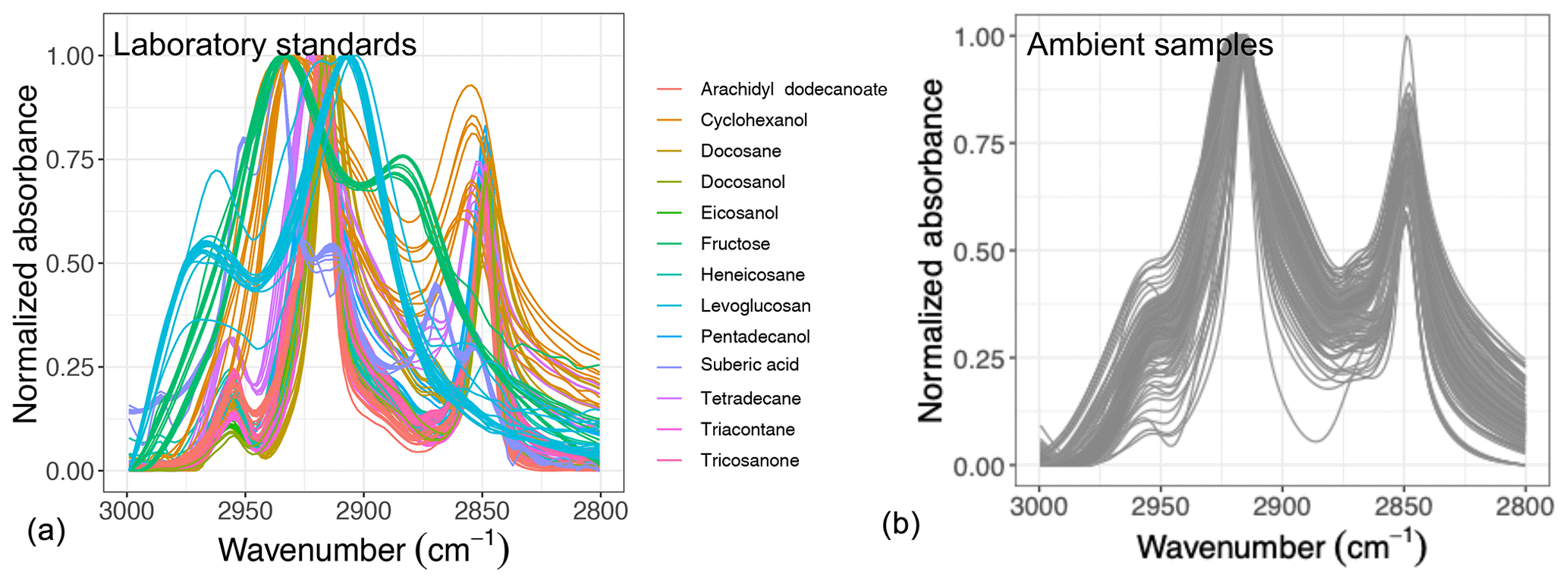
Figure 1Normalized aliphatic C−H spectra of the laboratory standards (a) and several atmospheric samples (b). This figure shows variation in absorbance profile among the standards and atmospheric samples.
Overall, the absorbance profile in the aliphatic C−H region contains direct and indirect information about carbon number and molecular weight and shows significant variation in laboratory standards and atmospheric samples (Fig. 1) related to their molecular structure. In this work, we adopt a new approach for using mid-infrared spectra to characterize OM. We use the variations in the aliphatic C−H region to estimate mean carbon number and mean molecular weight of atmospheric samples. In previous studies on the mid-infrared spectrum of atmospheric aerosols, functional group molar abundance in laboratory standards or total OC from other methods such as TOR were considered as the response variable, while non-normalized absorbances were considered as independent variables (Takahama et al., 2013; Ruthenburg et al., 2014; Reggente et al., 2016). In this manner, linear models resembling the Bouguer–Lambert–Beer law were developed. In this study, however, molecular weight and carbon number statistical models were developed using chemical formulas of the laboratory standards (no molar abundance information) and their normalized aliphatic C−H absorbances as independent variables. The current approach extracts detailed information from the mid-infrared spectrum complementary to previous approaches (Fig. 2).
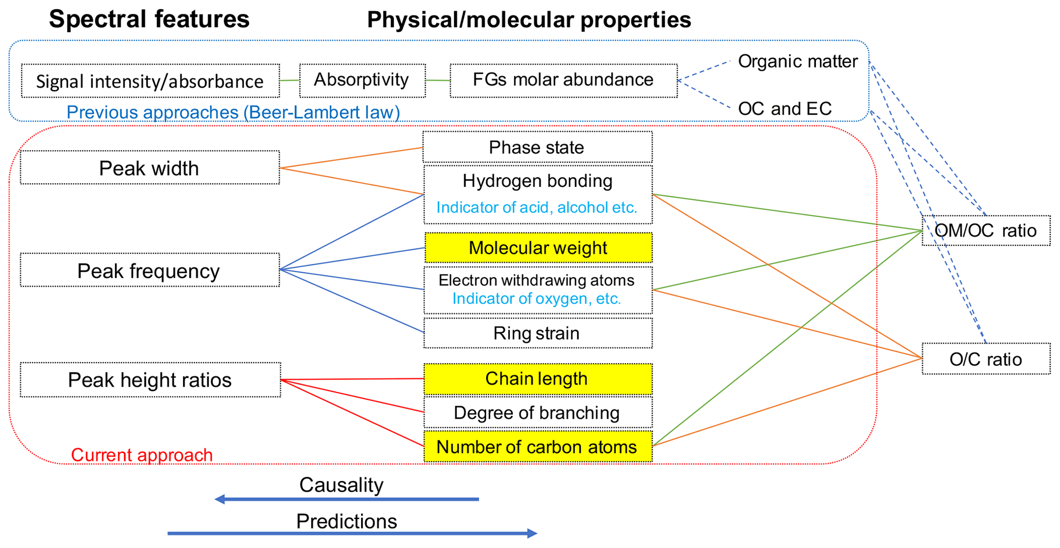
Figure 2Diagram showing the relation between spectral features and molecular or physical properties. The way previous approaches (e.g., Ruthenburg et al., 2014; Takahama et al., 2013) and the current approach use the mid-infrared spectrum to estimate different parameters is shown in blue and red boxes, respectively. Highlighted molecular properties can only be estimated using the current approach.
We will describe the atmospheric samples as well as the laboratory standards for the calibration and test set in Sect. 2.1 and 2.2. Thereafter, the methodology for data analysis and interpretation will be discussed in Sect. 2.3, 2.4, and 2.5.
2.1 IMPROVE network monitoring sites (sampling and analysis)
Particulate matter with diameter less than 2.5 µm (PM2.5) was collected on PTFE filters (25 mm diameter Teflo® membrane, Pall Corporation) every third day for 24 h, midnight to midnight, at a nominal flow rate of 22.8 L min−1 during 2011 and 2013 at selected sites in the IMPROVE network (http://vista.cira.colostate.edu/improve/, last access: 8 October 2020). There are, in total, 814 samples collected at 7 sites in the US in the year 2011 and 2161 samples collected at 16 different sites in the US 2013 (see Fig. 3). Overall, 1 out 7 sites in 2011 and 4 out of 16 of sites in 2013 are urban sites, and the rest are rural. FT-IR analysis was performed on the PTFE filters using a Bruker Tensor 27 FT-IR spectrometer equipped with a liquid nitrogen-cooled, wideband mercury–cadmium–telluride (MCT) detector and at a resolution of 4 cm−1 (data intervals of 1.93 cm−1; Nyquist sampling). For samples with low molar abundance of organic compounds, especially aliphatic C−H, baseline correction could not be done properly in the aliphatic C−H region, resulting in irregular and negative absorbance profiles. These samples were omitted from further analysis and only 798 were analyzed in this work. As can be seen from Fig. 4, data recovery is higher at urban sites than at rural sites due to a usually more prominent aliphatic C−H peak. Due to this undersampling, generalizing the results of this work to the whole of rural samples should be done with caution.
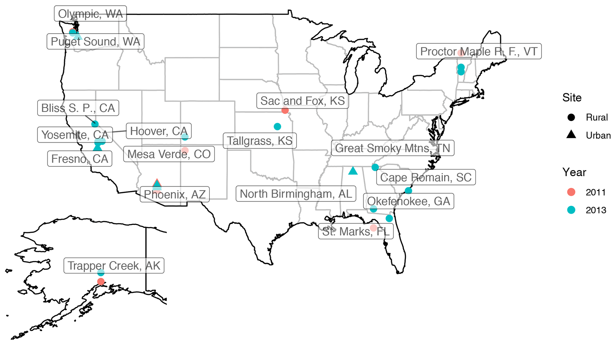
Figure 3The location of IMPROVE sites used for this work (the US and Alaska); the year in which samples are taken is differentiated by color and the type of the site by point shape.
2.2 Laboratory standards (sampling and analysis)
Compounds containing relevant functional groups to atmospheric OM such as aliphatic C−H, alcohol and acid O−H, carbonyl C=O, and with different structures (straight chain and cyclic) and various chain lengths were used to produce laboratory standards (Table 1). All compounds used for creating the standards contained aliphatic C−H, which is the main focus of this study. Five of these compounds were alkanes, just containing aliphatic C−H. Three were straight-chain alcohols containing alcohol O−H as well. One was cyclic alcohol, and one was a cyclic ketone having carbonyl C=O; two were cyclic (not aromatic) sugar derivatives containing several O−H groups. The calibration set also contained an ester, a ketone, and one dicarboxylic acid. In addition to relevance to atmospheric OM, these standards were selected based on the availability of spectroscopic data and their suitability for atomization. These compounds had comparable absorption coefficients for aliphatic C−H, and the effect of other functional groups, heteroatoms, and the molecular structure was analyzed indirectly via the change in the aliphatic C−H absorbance profile. Some of the laboratory standards and their resulting spectra were taken from Ruthenburg et al. (2014). The rest were created (using a similar protocol) from methanolic solutions with a concentration of 0.1 g L−1 and analyzed by FT-IR as follows. Atomized aerosols of the desired compounds were first generated by a TSI Model 3076 aerosol generator using the methanolic solutions. Then, these particles were conducted by the flow system towards a 47 mm PTFE filter (Teflo® membrane, Pall Corporation), where they were collected. The flow system was composed of a silica gel dryer (for drying the aerosols before collection), a sharp-cut-off 1 µm cyclone, and a diluter system (which facilitated the adjustment of aerosol concentration in the line). The pressure drop needed for the flow through the filter was provided by a rotary vacuum pump (Gast 0523-101Q-G588NDX), and the filter flow was controlled by a gas-flow controller (Alicat MCR-100-SLPM-D/5M). The mass on the filters ranged from few micrograms to tens of micrograms. After collecting the aerosols on the filters, FT-IR analysis was performed on the PTFE filters using a Bruker Vertex 80 FT-IR spectrometer equipped with a deuterated lanthanum α alanine doped triglycine sulfate (DLaTGS) detector, with the same spectral resolution as the spectra of the ambient samples.
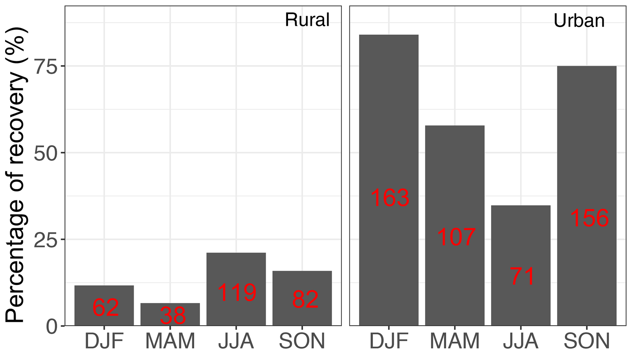
Figure 4Percentage of the samples which were recovered from each category (sample type and season) after baseline correction. The number of samples in each category is shown in red.
In total, 168 laboratory samples with different composition and molar abundance (absorption amplitude ranging from 0.001 to 2 before normalization) were used, from which a subset of 43 samples was kept as a test set and the rest were used as the calibration set. The test set was used solely for the purpose of evaluation of the statistical models developed using the calibration set. However, the final statistical models, which were applied to ambient samples, were developed using all 168 laboratory standards to increase the precision.
Table 1Chemicals used in the calibration set to analyze the effect of different physical or chemical properties of organic molecules on aliphatic C−H absorbance profile.

2.3 Baseline correction and normalization
The baseline removal is often a useful step in mid-infrared spectroscopy on PTFE filters, like in other methods of spectroscopy. The baseline arises from light scattering by the filter membrane (Mcclenny et al., 1985) and particles collected on the filter as well as electronic transitions of some carbonaceous materials (Russo et al., 2014; Parks et al., 2019). For baseline removal, we used the smoothing spline method on the 1500–4000 cm−1 region, where PTFE filter does not absorb, with parameter selection criteria similar to the approach taken by Kuzmiakova et al. (2016). Briefly, a cubic smoothing spline was fitted to the spectrum and then was subtracted from the raw spectrum to obtain the pure contribution of functional groups at each wavelength. The analyte region (the aliphatic C−H absorption region; 2800–3000 cm−1) was manually excluded from the baseline by setting the weights in this region to zero in the smoothing spline objective function (refer to Kuzmiakova et al., 2016). The rest of the spectrum between 1500 and 4000 cm−1 was included in the baseline by setting the weights to 1. After baseline correction, the aliphatic C−H absorbances were scaled between 0 and 1 (Fig. 1) for all spectra so that the absorbance profiles were comparable regardless of the absorbance intensity (functional group abundance).
2.4 Building the calibration models
In order to estimate molecular weight and carbon number from the normalized aliphatic C−H absorbances in the mid-infrared spectra, we seek the solution of the following linear equation for the calibration models:
where X is the normalized spectra matrix (the aliphatic C−H absorption region, 2800–3000 cm−1), y is the vector of response variable (molecular weight or carbon number), and e is a vector of residuals (y and X are assumed to be centered). In spectroscopic applications, due to indeterminacy (more independent variables than the number of samples) and collinearity (inter-correlation between independent variable), the ordinary least squares (OLS) method is not applicable or is not robust unless regularized. Among the common methods developed for treating such a data structure, we chose univariate (y is a vector, i.e., has one variable) partial least squares regression (PLSR) for this work (Wold et al., 1983). Univariate PLSR projects X onto P basis with orthogonal scores T and residual matrix E (Eq. 3) such that the covariance between each score column and y is maximized (in each step of deflation). Thereafter, the response variable y is regressed linearly against the scores (Eq. 4). In Eq. (4), c is the regression coefficient of y as a function of scores (T) and f is the vector of residuals.
Determining the optimum number of latent variables (LVs), which are linear combinations of original wavenumbers in this study, is an essential step for developing calibration models with predictive capability. After solving the PLSR problem for calibration models with different number of LVs, we ran a repeated 10-fold cross validation on the calibration models and calculated the root mean square error (RMSE) of predictions (for the calibration set) for each model. Thereafter, the model whose RMSE was within 1 standard error from the calibration model with minimum RMSE and had fewer LVs (i.e., a simpler model) was chosen (Hastie et al., 2009). Based on the above-mentioned procedure, the optimal number of LVs for molecular weight and carbon number calibration models was found to be 19 and 20, respectively.
2.5 Interpreting the calibration models using the basic spectral features
Although the PLSR models have considerably fewer LVs (approximately 20) than the original wavenumbers (105), the lack of physical interpretability and remaining number of LVs still hinders their physical interpretation. Therefore, we first analyze the basic (physically interpretable) features of the mid-infrared spectrum – peak frequencies, widths, and ratios in the aliphatic C−H region – for the calibration set and their relation with carbon number and molecular weight (Sect. 3.1). Spatial and temporal variations of these patterns in the atmospheric samples are also analyzed and related to similar patterns in the laboratory standards.
The four basic features of the ambient sample spectra were used to build a classification and regression tree (CART) (Breiman et al., 1983) to approximate the PLSR predictions of mean molecular weight and carbon number and to better understand their connection with the underlying spectral absorption characteristics. In this approach, binary decision trees are generated to classify the PLSR estimates based on partitioned domains of their basic spectral features. The CART algorithm expands the trees in the order of decreasing explanatory power until certain stopping conditions (e.g., minimum number of observations in terminal nodes or minimum improvement of explanatory power at each step of splitting) are satisfied.
First, the basic features of the aliphatic C−H profile are discussed in the atmospheric and the laboratory samples, followed by a similarity check between the two (Sect. 3.1). Then, development of calibration models for predicting molecular weight and carbon is described, followed by investigation of their performance in the calibration and test (Sect. 3.2). Thereafter, the model estimates are discussed for atmospheric samples and compared to the results reported in literature (Sect. 3.3). Finally, the basic features introduced earlier are used to classify the results of the sophisticated (PLSR) models in order to obtain a better understanding of the way they function (Sect. 3.4).
3.1 Basic features
Basic features of the spectrum in the aliphatic C−H region were calculated for atmospheric samples and laboratory standards to study their temporal and spatial variation and their relation with molecular properties such as molecular weight, carbon number, and the ratio. These variables, although few, can give a good estimate of the absorbance profile and make it more interpretable.
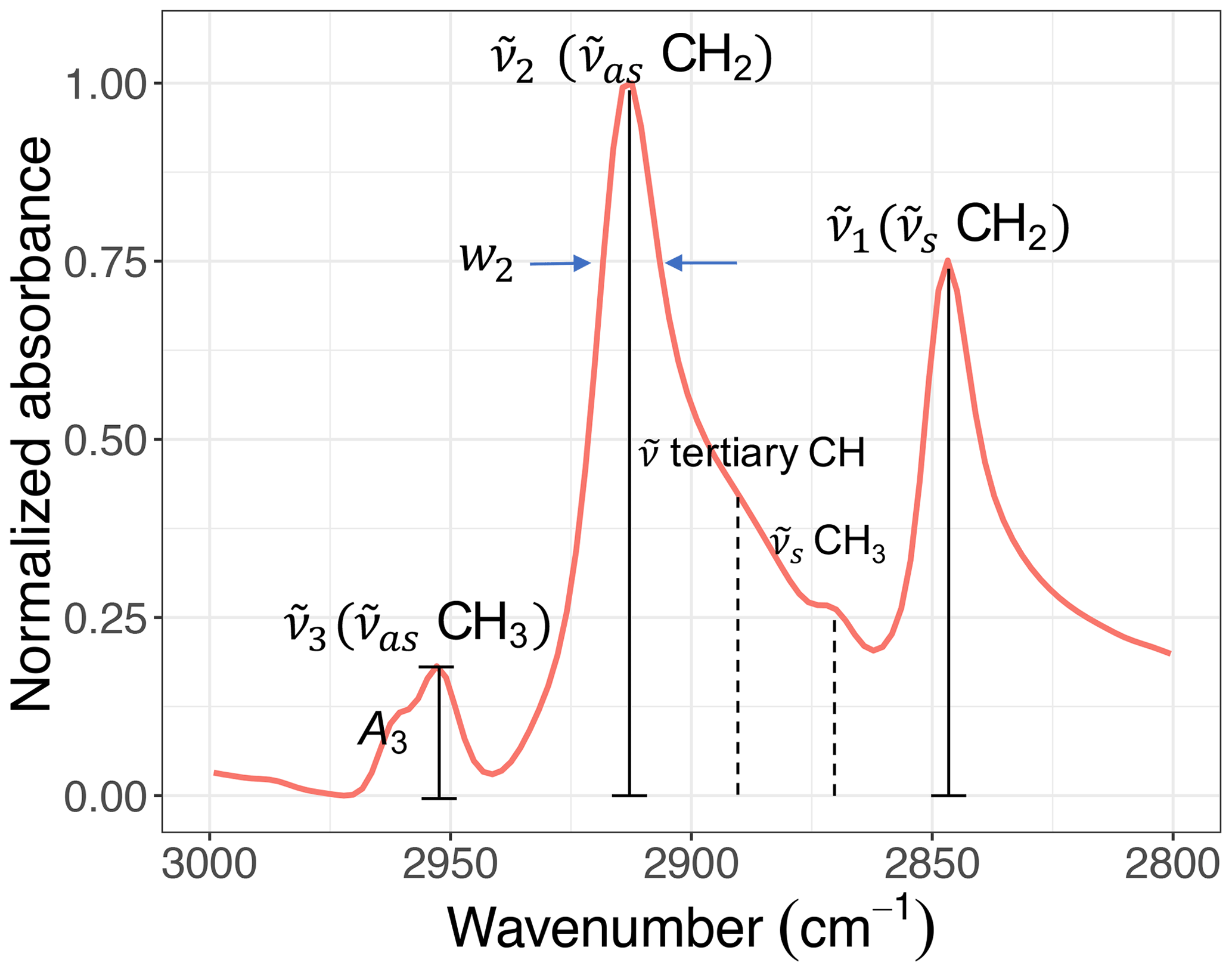
Figure 5A sample C−H spectrum showing the convention of peak parameters used in this study. The symmetric CH2 ( CH2) wavenumber is denoted by . The asymmetric CH2 ( CH2) wavenumber is denoted by and the asymmetric CH3 ( CH3) wavenumber by . Absorbance and width of the ith peak are also denoted by Ai and wi, respectively.
Figure 5 shows the convention of spectral features in the aliphatic C−H (2800–3000 cm−1) region used in this study. Apart from methine group (tertiary C−H), which has a very weak absorption (Pavia et al., 2008), there are two doublets in this region corresponding to CH2 and CH3 symmetric and asymmetric stretching vibrations. The CH3 symmetric peak is typically suppressed by the surrounding peaks and is not completely distinguishable. Among the remaining peaks, the symmetric CH2 ( CH2) wavenumber is denoted by . Likewise, the asymmetric CH2 ( CH2) wavenumber is denoted by and the asymmetric CH3 ( CH3) wavenumber by . Absorbance and peak width of the ith peak are also denoted by Ai and wi, respectively.
In the next subsections, the variations of the mentioned spectral features are studied in the laboratory standards and atmospheric samples. For this purpose, the atmospheric samples are separated into urban, rural, and burning categories. The burning category constitutes 95 samples of urban or rural sites and is taken from clusters 9a, 9b, and 10 of Bürki et al. (2020) based on their spectral similarity. These samples are believed to be influenced by residential wood burning or wildfires since they were usually collected during a known fire period (Rim Fire in California in 2013) or in Phoenix, AZ, during winter months when residential wood burning typically occurs (Pope et al., 2017).
3.1.1 Asymmetric CH2 peak wavenumber ()
We calculated the second peak wavenumber () for the laboratory standards and atmospheric samples using a simple peak-finding algorithm based on the first and second numerical derivatives of the spectrum. For the laboratory standards, the frequency generally decreases with increasing molecular weight until it reaches an asymptotic state after 200 g mol−1 (Fig. 6). The curve in Fig. 6 shows the theoretical peak frequency of the aliphatic C−H when the bond spring constant is assumed to be 103 N m−1 (Pavia et al., 2008), and the reduced mass is calculated based on a ball-and-string assumption composed of the hydrogen atom (first “ball”) and the rest of molecule (second “ball”). The only effect considered in this model is the variation of the reduced mass of the oscillator. The fact that the less-oxygenated laboratory samples follow the theoretical line closely implies that the value of the spring constant considered here is, on average, a good approximation. However, especially for highly oxygenated (high ratio) molecules and those with in liquid phase (which have a lower molecular weight), the absorption frequency deviates from the theoretical line (higher frequency) due to higher levels of intermolecular interaction.
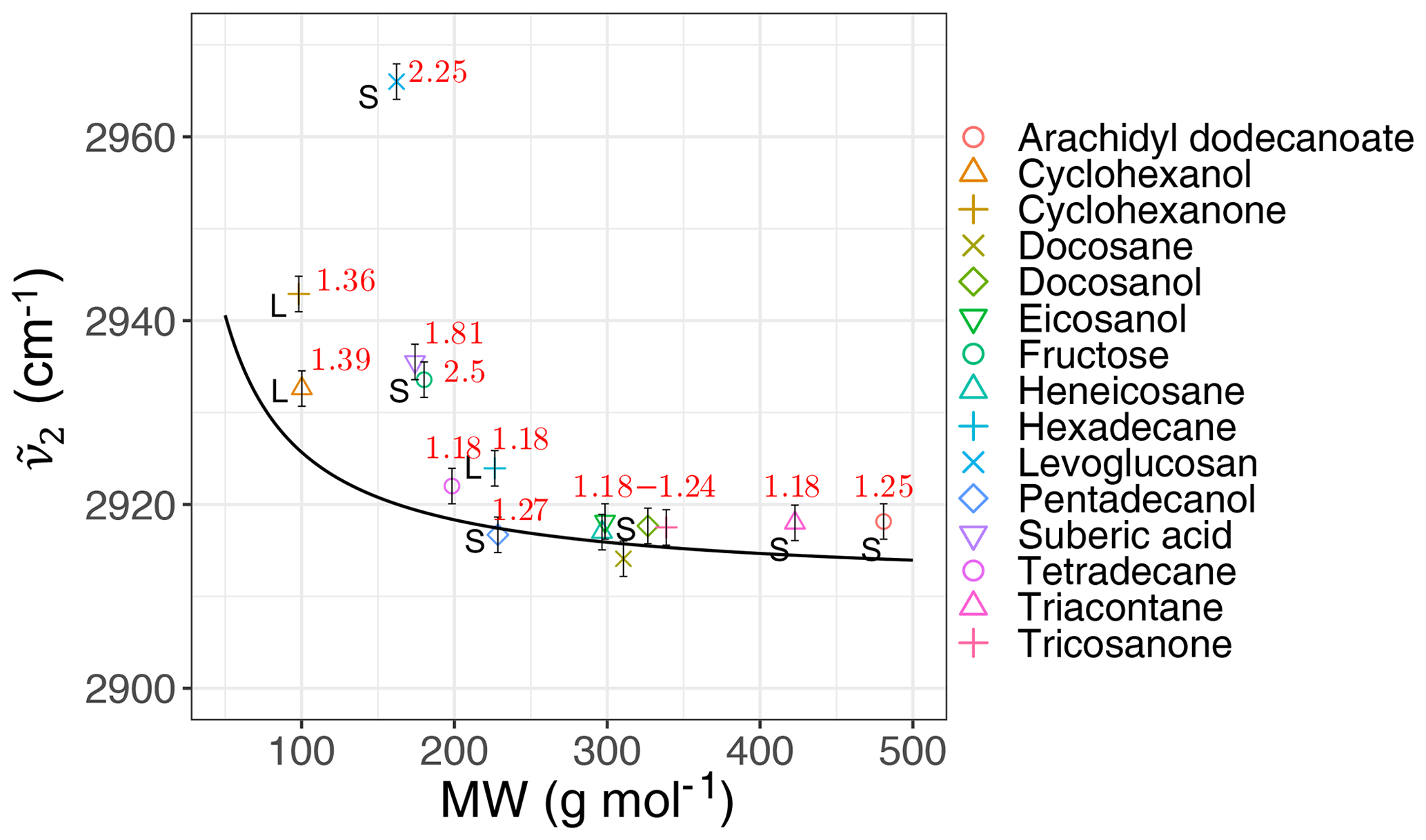
Figure 6Scatter plot showing the variation of the second peak wavenumber () with molecular weight (MW) in the calibration set, affected by the ratio and phase state. The black line shows the theoretical frequency with a spring constant equal to 103 N m−1 for all C−H bonds. The ratio and phase state are shown for the samples. The error bars show uncertainty in calculated peak frequency due to FT-IR scan resolution.
Regarding the atmospheric samples, most of categories have a peak density in 2915–2925 cm−1, close to that of straight-chain molecules of the laboratory standards (Fig. 7, first row). Urban samples have a wider shoulder on the right side (around 2925 cm−1) in summer when the samples are expected to be more aged. Other variations are believed to be insignificant considering the scan resolution of the FT-IR instrument.
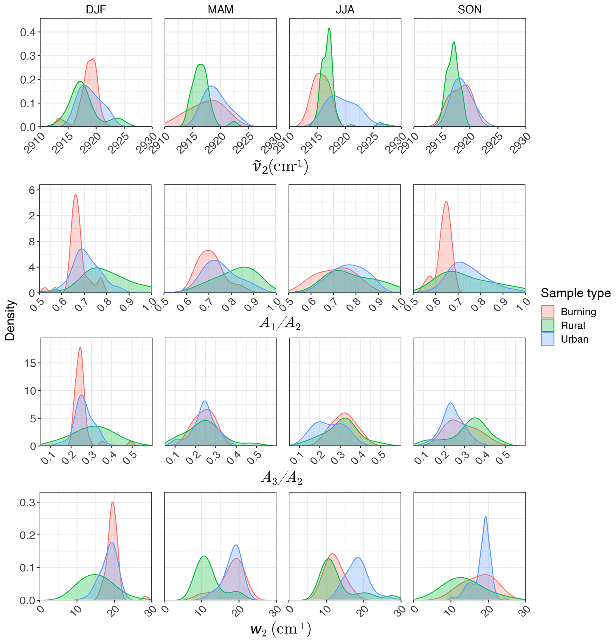
Figure 7Kernel density estimate of second peak wavenumber (), the ratio of peak heights of symmetric CH2 to asymmetric CH2 stretching (), the ratio of peak heights of asymmetric CH3 to asymmetric CH2 stretching (), and the second peak width (w2) of the aliphatic C−H band in the mid-infrared spectra of the atmospheric samples segregated based on sample type and season.
3.1.2 Peak height ratios ()
Analyzing the laboratory standards shows that a relatively linear but scattered relation exists between carbon number and the ratio in the calibration set (Fig. 8a). Suberic acid, which is the only dicarboxylic acid in the laboratory standards, does not follow the general trend, probably due to strong dimerization. As mentioned in Sect. 1.2, the ratio compares symmetric and asymmetric absorbance of methylene, and its connection with carbon number has already been highlighted in FT-IR analysis of some types of diesel fuels (Price et al., 2017). Increase in is also observed between solid and liquids, consistent with the work of Corsetti et al. (2017). We also observe a nonlinear relation between the ratio and carbon number with different levels based on branching and terminal functionalization (Fig. 8b). This ratio is equal to zero for molecules lacking methyl group such as simple cyclic molecules while increasing as the number of branches containing terminal methyl increases.
Results show a clear separation in atmospheric samples regarding the sample type and season for both and ratios (Fig. 7, second and third row). The samples influenced by burning usually have the lowest ratio (Fig. 7, second row). This observation is consistent with the presence of molecules with longer chains, as observed for laboratory samples. Bürki et al. (2020) showed that the urban samples (in the same dataset) have their highest average ratio in summer which is concurrent with their highest ratio, which suggests shorter chain length. The highest ratio for rural samples is observed in spring when the aerosols are highly oxidized (Bürki et al., 2020). This suggests that aged aerosols have lower carbon number probably due to the fragmentation process. The measured ratio for the majority of the atmospheric samples ranges between 0.6 and 0.8, which is consistent with the value for laboratory standards. Results also show that the ratio is higher in rural samples compared to urban samples (with the exception of spring), suggesting a higher CH3 to CH2 abundance in those samples. This observation can be due to lower carbon number or higher number branches containing CH3. Like the ratio, we observe fewer samples with low ratios at urban sites in summertime. The ratio falls between 0.1 and 0.4 for the majority of the atmospheric samples, which is consistent with the value for laboratory standards. It is worth noting that peaks in atmospheric samples are more overlapped than laboratory standards, which makes calculation of peak ratios based on extrema of the original spectra imprecise. As a result, a peak-fitting method based on Gaussian peaks was applied to atmospheric samples in order to obtain the peak ratios more precisely.
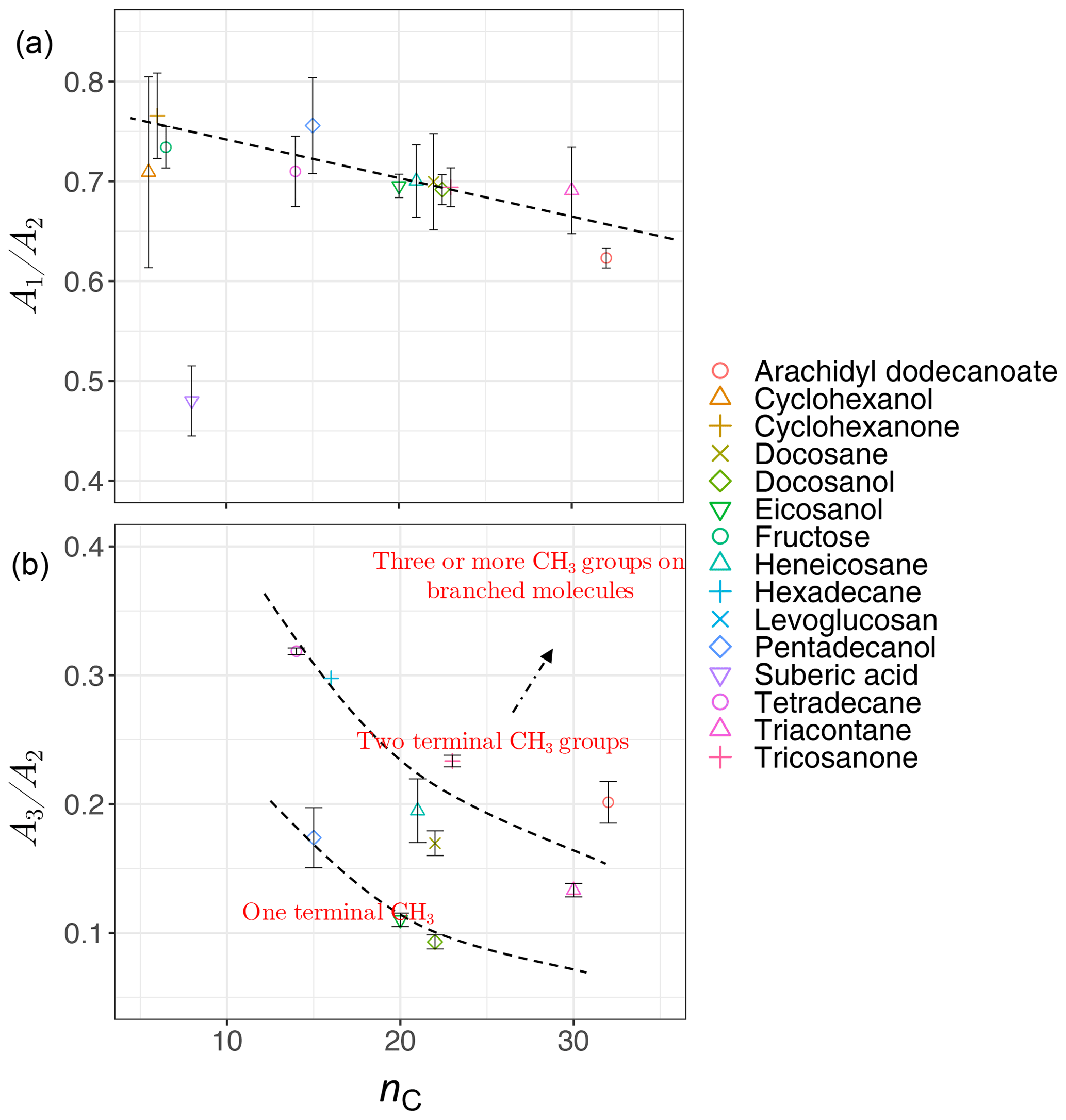
Figure 8Scatter plots showing the relation between carbon number (nC) and the ratio of peak heights of symmetric CH2 to asymmetric CH2 stretching (, a), and the ratio of peak heights of asymmetric CH3 stretching to asymmetric CH2 stretching (, b), averaged for each substance in laboratory standards. Error bars show ± 1 standard error from the average, and dashed lines are visual guides for the trends and levels.
3.1.3 Peak width (wi)
We observe a clear correlation between w2 and the ratio in the calibration set when solid and liquid phases are considered separately (Fig. 9). As mentioned in Sect. 1.2, hydrogen bonding increases the peak width, and the extent of hydrogen bonding is usually a good indicator of the ratio. This is because hydroxyl, hydroperoxyl, and carboxyl groups, which form hydrogen bonds, are among the most effective functional groups in secondary organic aerosol (SOA) formation due to the significant vapor pressure reduction they cause (Seinfeld and Pandis, 2016). In this study, w2 is defined as the peak width at 75 % of the maximum amplitude. This position is chosen for robustness of the measurement algorithm (to avoid interference with other peaks); however, it can be converted to full width at half maximum (FWHM) assuming the proper peak profile (w2 is 65 % of FWHM for a Gaussian peak). In addition to hydrogen bonding and phase state, superposition of a multitude of peaks with slightly different profiles can also have a statistical positive or negative effect on the peak width in mixtures (see Sect. S1 in the Supplement). The observed peak width in the mid-infrared spectra of the atmospheric samples is the result of all above-mentioned factors. However, since all laboratory standards are produced with pure compounds, the significance of the mixture effect cannot be evaluated.
Figure 7 (fourth row) shows a distinct distribution of w2 considering spatial and temporal variations as well as sample category. Rural samples have a smaller value of w2 compared to urban and burning samples, although the former are usually more oxidized (have higher ratio). This observation suggests that other factors such as phase state and statistical effects likely outweigh the oxygenation effect on absorption peak width.
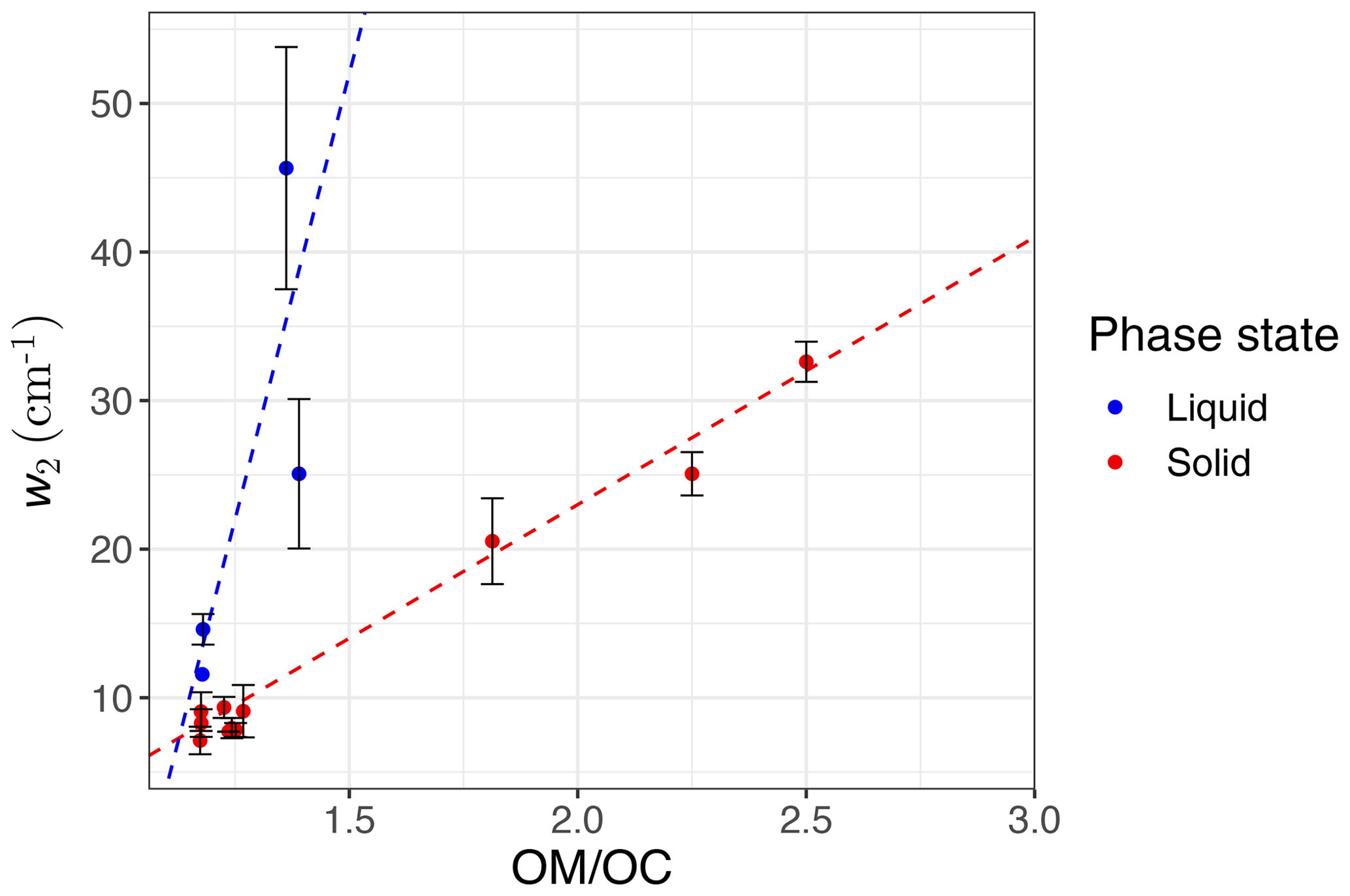
Figure 9The average value of second peak width (w2) measured for each compound in the calibration set versus the ratio, colored based on compound phase state at laboratory condition (25 ∘C). Error bars show ± 1 standard error from the average, and dashed lines are visual guides.
3.1.4 Spectral similarity (dimension reduction)
In previous sections, the basic features of spectra in the aliphatic C−H region were presented and discussed for the atmospheric samples and laboratory standards. Here, we check the spectral similarity between atmospheric complex mixtures and laboratory pure standards by means of principal component analysis (PCA), before developing calibration models.
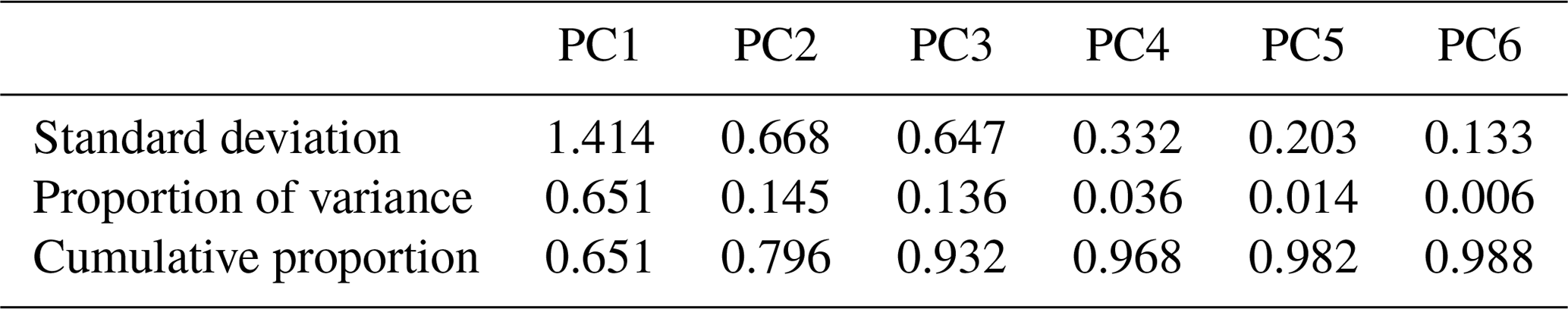
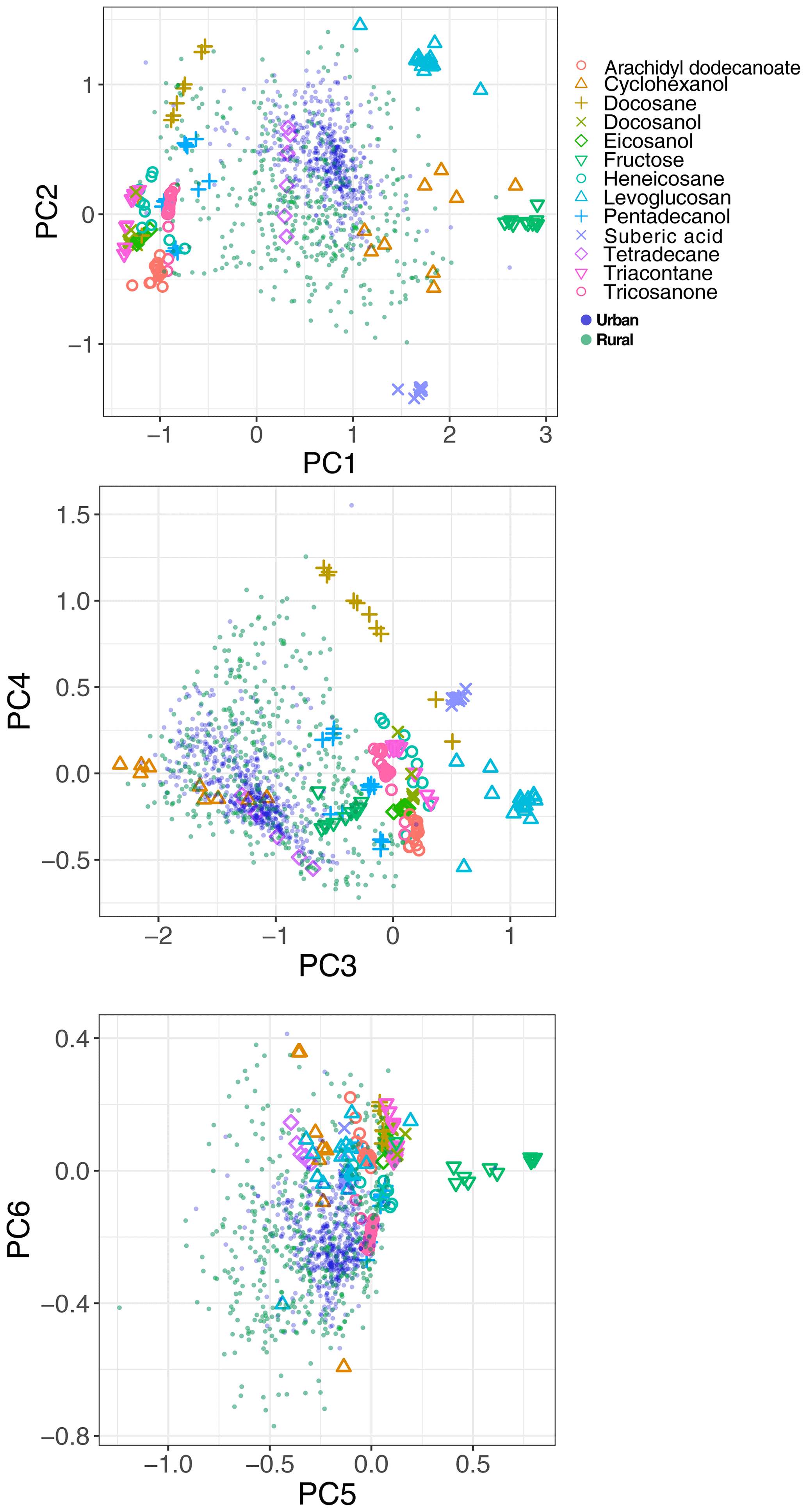
The spectral data of laboratory standards are highly collinear as can be seen from their correlation matrix heat map (Fig. A1). In this case, PCA is efficient for reducing the data dimension such that only the first six principal components (PCs) explain around 99 % of variance in the spectra (Table 2). For the sake of comparison, we have projected the spectra of atmospheric samples onto the six PCs. The results show that their scores, when projected onto laboratory PCs, are surrounded by laboratory standards. Many spectra, particularly urban ones, are clustered close to tetradecane for the first four PCs (Fig. 10); greater differentiation is found among the higher PCs. This observation suggests that the laboratory standards are able to capture the main variations in the spectra of atmospheric samples, which have a more regular aliphatic C−H profile close to that of straight-chain alkanes. We also found that PC3 appears to capture phase state information (see Sect. S2).
Table 2Importance of the first six principal components in the laboratory standards.
3.2 Developing and evaluating the calibration models
PLSR with cross validation was used to develop quantitative models for molecular weight (MW) and carbon number (nC) with the calibration set composed of 143 samples including all compounds over the available mass range. The ratio was then calculated from these two parameters (). The developed PLSR models gave reasonably good fit results (r2 ranging from 0.94 to 0.99) for molecular weight, carbon number, and indirect ratio in the calibration set (Fig. 11).
The prediction ability of the PLSR models was then evaluated using a test set composed of 43 samples which were not used for developing the models. The PLSR models also performed reasonably well in predicting molecular weight, carbon number, and ratio in the test set with r2 ranging from 0.92 to 0.98 (Fig. 11). The predictions with high relative error were attributed to laboratory samples with low molar abundance (low signal-to-noise ratio), for which the baseline correction had the highest uncertainty. This is not a concern when applying the PLSR models to atmospheric samples since the atmospheric samples with low signal-to-noise ratio were omitted in the first step (Sect. 2.1).
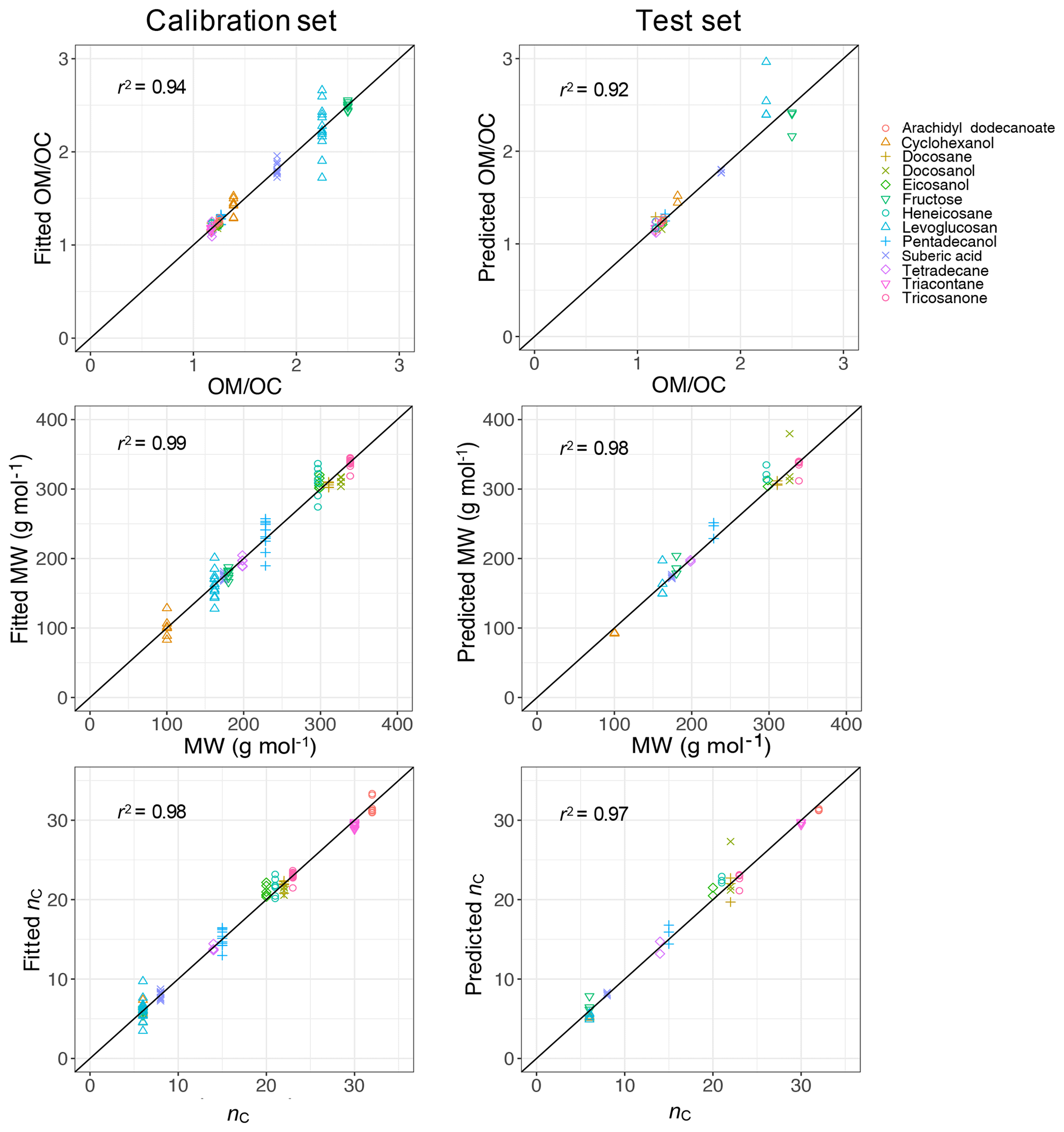
Figure 11Scatter plot of fitted (predicted) indirect ratio, MW, and nC against the values from chemical formula of the calibration set (test set). The diagonal black lines indicate the perfect fit (1:1).
3.3 Applying the calibration models to atmospheric samples
After checking the performance of the PLSR models on the calibration and test set, all laboratory standards were used to build calibration models that were applied to the ambient samples. In the following sections, the estimates of , mean molecular weight, and mean carbon number for the ambient samples are shown in different categories based on season and sample type (rural, urban, and burning) after omitting the physically unreasonable values. Thereafter, the trends and absolute values are compared to previous studies (when available) and our expectations based on aging process and aerosol emission sources.
In this work, we have assumed that we can obtain mean mixture (atmospheric samples) properties from the normalized spectrum of a mixture using the calibration models developed for pure compounds (laboratory standards). This assumption relies on the linearity of the property estimation models (which is consistent with our calibrations; Eq. 4) and equality of the absorption coefficients of the compounds existing in the mixture (see Appendix B for more information). Thus, the absorption coefficient of aliphatic C−H has been assumed to be relatively similar between the compounds existing in atmospheric samples. Although the aliphatic C−H absorption coefficients of the laboratory standards were similar in this study, the variability of this absorption coefficient is relatively less studied for compounds existing in the atmospheric OM and needs to be addressed in the future. This assumption is a potential source of error that may change the accuracy of the results, but the estimates for atmospheric samples shown in the following sections suggest that this assumption does not overwhelm the findings.
3.3.1 ratio
The ratio is the first parameter that we investigate here since it has been studied extensively in atmospheric aerosols (Bürki et al., 2020; Hand et al., 2019; Ruthenburg et al., 2014; Takahama et al., 2011; Simon et al., 2011; Aiken et al., 2008). Moreover, it can be used as an indirect evaluation for mean molecular weight and mean carbon number estimates as the indirect ratio is calculated from those two. An indirect estimate that is consistent with previous studies implies that estimates of molecular weight to carbon number are also likely to be reasonable.
The ratio is estimated to be generally lower for urban samples (≈1.5) than rural samples (≈1.8; Fig. 14, first row). The lower ratio at urban sites is thought to be related to emission sources that are generally hydrocarbon, with low ratio emitted from gasoline and diesel vehicles (fuel combustion and unburned motor oil) as a major part of anthropogenic SOA precursors (Gentner et al., 2012), as well as cooking. These organic molecules do not undergo significant oxidation and aging as the monitoring sites are generally close to the emission sources. In contrast, organic aerosols usually undergo several steps of oxidation and receive substantial condensation of oxidized vapors, which results in higher ratio at rural and remote sites. Previous studies using several different methods (including FT-IR and AMS) show the same trend at urban and rural sites (Ruthenburg et al., 2014; Zhang et al., 2007; Simon et al., 2011; Bürki et al., 2020). In addition, the majority of the samples are in the range that is usually considered for ratio, i.e., 1.4–1.7 (Russell, 2003). We also observe that samples influenced by burning, especially residential wood burning, have lower ratio (≈1.4) than those associated with more oxidized aerosol such as rural sites, consistent with estimates of Bürki et al. (2020).
The ratio at urban sites is estimated to be higher in summer compared to other seasons, especially winter (Fig. 14, first row) which is believed to be caused by more intense photochemical aging in summertime (Kroll and Seinfeld, 2008). At rural sites, the trend becomes more complicated, as vegetation, a major biogenic SOA emission source, is more active in summertime (Yuan et al., 2018; Seinfeld and Pandis, 2016). Samples influenced by burning are also estimated to have higher in summer when samples are affected by wildfires compared to winter when burning samples are mostly affected by residential wood burning. However, the contribution of photooxidation relative to emission sources is not clear in this case, as they are coupled in these observations (Bürki et al., 2020).
In order to have a direct comparison with other methods, we chose the Phoenix, AZ, monitoring site, for which recovery percentage of the baseline correction method is close to 100 %, and compared our indirect ratio estimates to the corresponding ones calculated by Bürki et al. (2020). The latter method uses molar abundance information of functional groups in laboratory standards in addition to a much wider region of non-normalized mid-infrared spectrum (1500–4000 cm−1). The median seasonal ratios of this study underpredict that of Bürki et al. (2020) by 0.12 on average, while reproducing the same temporal trends. Some of the discrepancies may be due to insensitivity of spectral features to molecular characteristics in certain domains – for instance, the variation of peak frequency diminishes with increasing molecular weight (Sect. 3.1.1). However, the overall agreement between the two methods is reasonable considering the indirect nature of estimates in our work (Fig. 12).
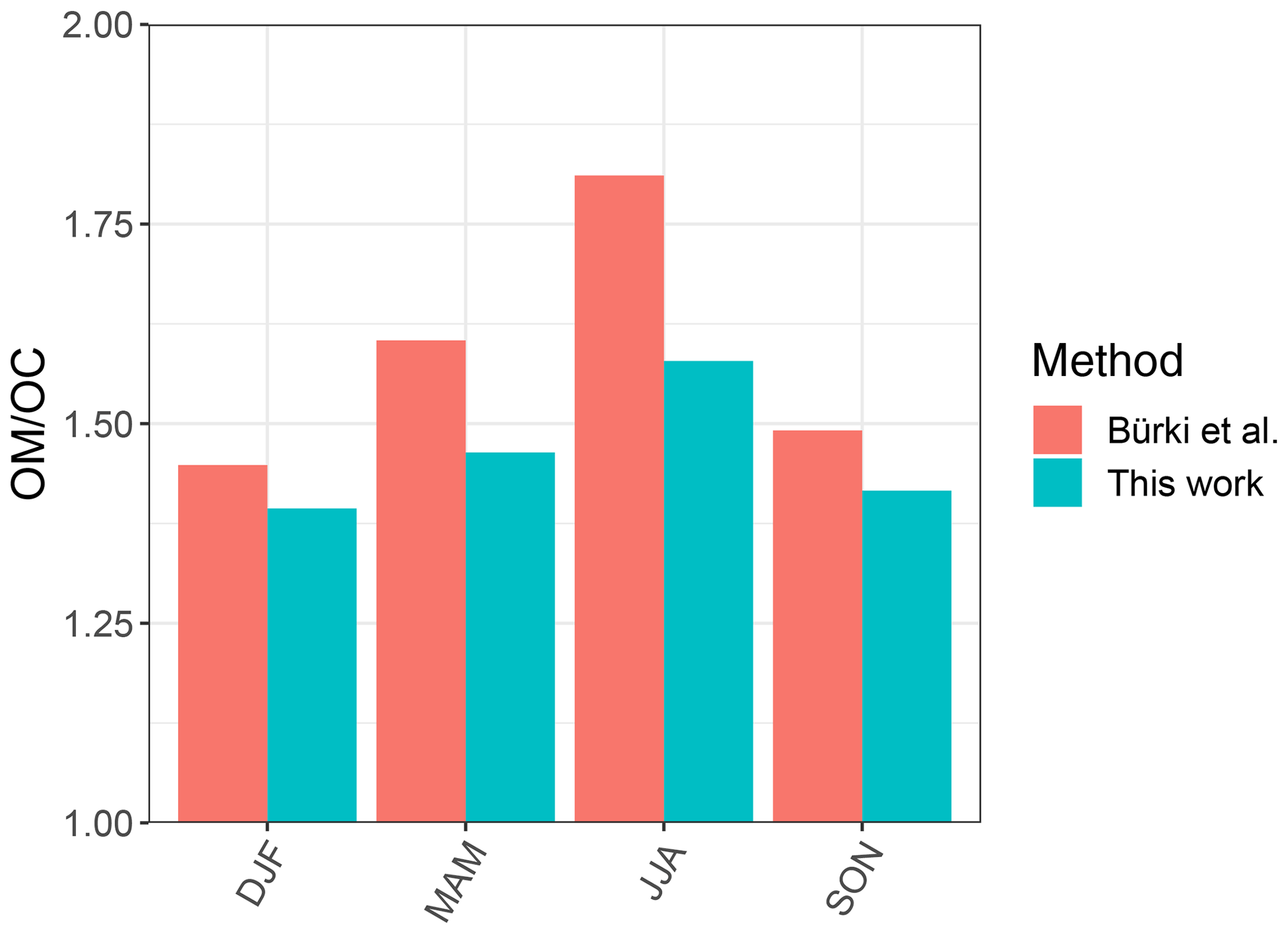
Figure 12Bar chart showing median ratio calculated for each season based on samples collected at the Phoenix, AZ, monitoring site using our method and the one used by Bürki et al. (2020).
3.3.2 Molecular weight
The PLSR model estimates the mean molecular weight to range between 100 and 350 g mol−1 for the majority of the samples (Fig. 14, second row). To the best of the authors' knowledge, no extensive study has been performed on mean molecular weight of ambient organic aerosol constituents. Nevertheless, the estimated range is reasonably close to that of the studies that have been done. Those studies measured molecular weights up to 200 g mol−1 for SOA constituents using GC/MS and ion chromatography (Cocker III et al., 2001; Jang and Kamens, 2001b; Kalberer, 2004), an average molecular weight between 200 and 300 g mol−1 for atmospheric humic-like substances (HULIS) using electro-spray ionization (ESI) (Graber and Rudich, 2006), and an average molecular weight between 300 and 450 g mol−1 for oligomers formed in a smog chamber, measured using laser desorption/ionization mass spectrometry (LDI-MS) (Kalberer et al., 2006). Although particle-phase oligomerization processes result in high-MW compounds (Jang and Kamens, 2001a; Tolocka et al., 2004; Shiraiwa et al., 2014), the abundance of these compounds is usually debated since the available experimental results regarding the reversibility of accretion reactions are contradictory (Kroll and Seinfeld, 2008). Moreover, oligomer formation may be overestimated in laboratory conditions compared to atmospheric particles (Kroll and Seinfeld, 2008; Kalberer, 2004; Trump and Donahue, 2014).
The PLSR molecular weight model estimates a lower mean molecular weight for rural samples (≈200 g mol−1) compared to urban ones (≈240 g mol−1), while burning samples are estimated to constitute the heaviest molecules (≈290 g mol−1). This observation is consistent with our knowledge of emission sources. Emissions in urban areas are influenced by long-chain hydrocarbons from combustion products and motor oil (Gentner et al., 2012), while biomass burning is accepted to be the primary source of high-MW HULIS (Li et al., 2019). We also observe a decrease in mean molecular weight peak density in urban samples from winter to summer that is believed to be attributed to fragmentation during more intense photooxidation in summer (Hand et al., 2019; Jimenez et al., 2009) for emission sources that do not change drastically between the two seasons. The same phenomenon is observed in LDI mass spectra of some urban samples in summer and winter reported by Kalberer et al. (2006). Although the reduction in mean molecular weight due to fragmentation can be compensated for by addition of heavy atoms to the molecule during oxidation, our results suggest that the overall direction of photooxidation at urban sites is reduction of the mean molecular weight.
3.3.3 Carbon number
The PLSR carbon number model estimates that the recovered rural samples usually have lower mean carbon number compared to urban samples and the samples influenced by burning (Fig. 14, third row). Higher mean carbon number estimates at urban sites (highest probability density around 16), which are coincident with high elemental carbon (EC) values from TOR measurements (Fig. C1), can be attributed to major EC sources such as combustion of fossil fuel and biomass. This is also consistent with high SOA formation potential of molecules with 15–25 carbon in diesel fuel shown by Gentner et al. (2012). Samples affected by burning are estimated to have the highest mean carbon number among all samples. This observation is consistent with the emissions of plant cuticle waxes, mainly composed of straight-chain hydrocarbons, observed during biomass burning (Hawkins and Russell, 2010) as well as HULIS (Graber and Rudich, 2006). We also observe a decrease in estimated mean carbon number of urban samples from winter to summer, suggesting fragmentation during aging and photooxidation processes.
The carbon–oxygen estimates of the PLSR models are consistent with the existing numerical simulation. We compared our estimates with the numerical simulations by Jathar et al. (2015). A multi-generational oxidation model used by Jathar et al. (2015) (Statistical Oxidation Model, SOM, in a 3-D air quality model) for simulating SOA in Los Angeles and Atlanta (two urban locations) shows that carbon number in SOA ranges from 3 to 15 with the concentration peaks around 7, 10, and 15 (Fig. 13). For this comparison, we calculated the carbon–oxygen grid from our molecular weight and carbon number estimates, assuming the organic molecules have a chemical formula of (a common assumption and one used by Jathar et al., 2015). Our PLSR models for the IMPROVE network estimate mean carbon number peaks (number density) for rural, urban, and burning samples to be around 8, 16, and 18, respectively, while the total range is limited to 3–19 (Fig. 13). We also estimate the oxygen number to range from 2 to 6 for the majority of the samples. It should be noted that this is an order of magnitude comparison since the time frame and the location of the two studies are different and the numerical simulation by Jathar et al. (2015) only considers SOA.
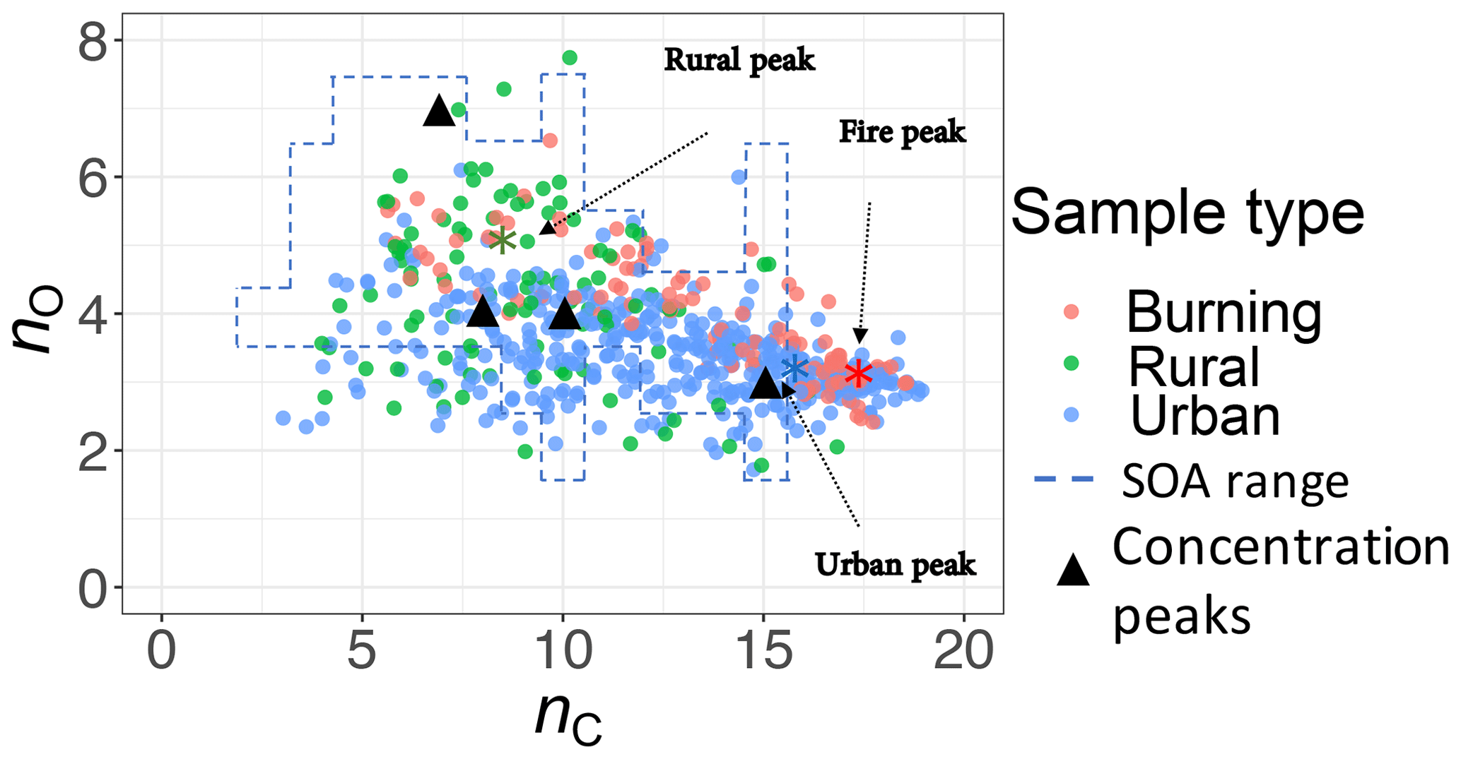
Figure 13Comparison between the carbon–oxygen grid simulated by Jathar et al. (2015) for Atlanta and Los Angeles with sample points estimated for the IMPROVE network (2011 and 2013) from the molecular weight and carbon number estimates of this study. The dashed lines show the range of simulated carbon and oxygen, and the triangles indicate the location of the highest SOA concentrations for the simulations of Jathar et al. (2015).
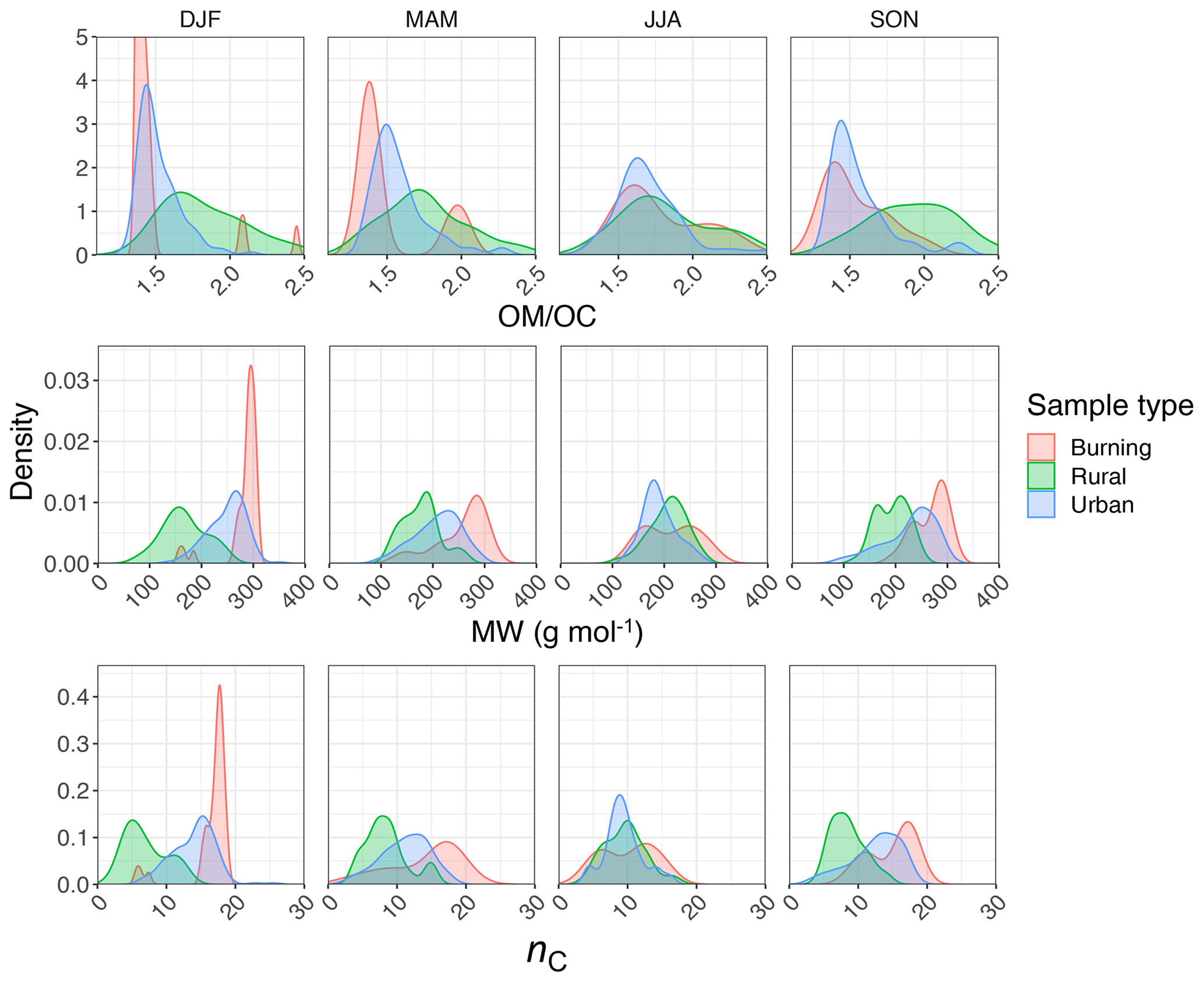
Figure 14Kernel density estimates of indirect ratio, MW, and nC estimated from normalized aliphatic C−H mid-infrared absorbances by PLSR models (segregated by sample type and season).
3.4 Calibration model interpretation
Reducing the spectrum to four basic features introduced in Sect. 3.1 (, , , w2) is a manual data compression onto a basis set of interpretable variables. Though information loss is inevitable, it was shown in Sect. 3.1 that these basic features are still sufficient for qualitative explanation of spectral variations associated with different emission source and aerosol aging process. In this section, predictions made by the PLSR models on the ambient samples are grouped based on the four basic features using CART (Fig. 15) in order to form a better understanding of how the sophisticated PLSR models function.
The regression trees show that the peak ratios are observed to be the main grouping parameter for both carbon number and molecular weight (Fig. 15). The inverse relation of peak ratios with carbon number appears in most of the splitting nodes of carbon number and molecular weight regression trees (Fig. 15). This is consistent with the observed relation between carbon number and peak ratios in the calibration set (Fig. 8). Assuming that molecular weight is highly correlated with carbon number, the classification of molecular weight based on peak ratios is also expected. The peak frequency () appears once as a node in molecular weight tree and classifies the estimates based on the same trend that was observed in the calibration set (Fig. 6). The second peak width (w2) also appears few times in the nodes, probably adding information about the ratio and phase state. The two trees shown in Fig. 15 explain only around 50 % of the variation of estimates made by the PLSR models. The explained variation can be increased to an arbitrarily high number through the use of more branches in the fitting dataset, but the predictive capability of regression trees for new samples depends highly on their similarity to the training set. In summary, regression trees show that the predictions of the PLSR models are generally consistent with the observed trends of the basic features in the calibration set (Sect. S3 supports this conclusion for individual spectra for which the PLSR models estimate quite different parameters). This observation implies that the PLSR predictions of carbon number and molecular weight are not independent of these basic features. However, the sophisticated PLSR models use other fine features in addition to the mentioned basic features to extract more detailed information and to reduce variabilities stemming from different sources such as baseline correction.
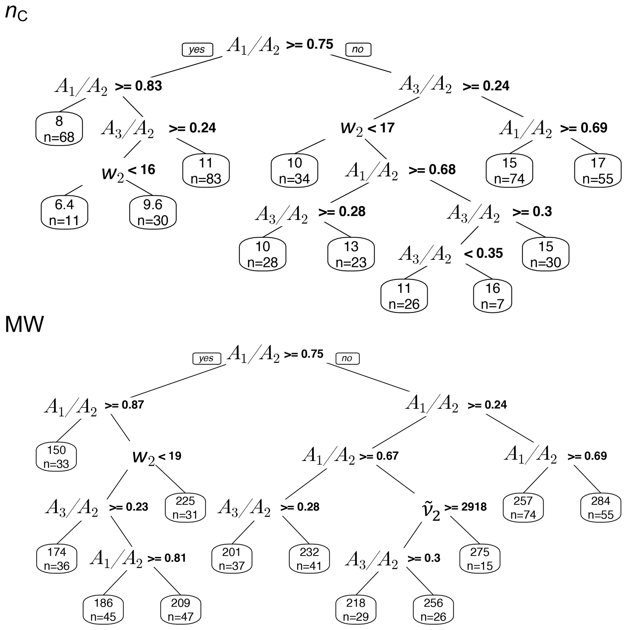
Figure 15Regression tree of MW and nC estimates in atmospheric samples based on the basic spectral features: second peak frequency (), the ratio of peak heights of symmetric CH2 stretching to asymmetric CH2 stretching (), the ratio of peak heights of asymmetric CH3 to asymmetric CH2 stretching (), and second peak width (w2) of aliphatic C−H band.
Normalized aliphatic C−H absorbances in the mid-infrared spectrum were used in this study to estimate carbon number and molecular weight of the atmospheric OM. First, it was shown that the spectral features, such as peak frequencies and ratios are correlated with carbon number, molecular weight, and the ratio for laboratory standards. We also observed a meaningful temporal and spatial variation of those features in atmospheric aerosol samples. Thereafter, PLSR models were developed on laboratory standards to estimate the mentioned parameters in the atmospheric aerosol samples from the IMPROVE network. The estimated molecular weight and carbon number reconstruct the values in the atmospheric aerosols that are consistent with previous studies with a reasonable difference (an average underprediction of 0.12). These new statistical models estimate lower mean carbon number and mean molecular weight in more aged aerosols of the same source highlighting the fragmentation role in aging process (Murphy et al., 2012). Moreover, they estimate relatively less oxidized, heavier molecules with higher carbon number for samples influenced by burning. The findings show that the new technique can help us better understand characteristics of OM due to source emissions and atmospheric processes. In addition, since carbon number and molecular weight are important characteristics used by recent conceptual models or parameterizations (e.g., Shiraiwa et al., 2017a; Li et al., 2016; Pankow and Barsanti, 2009; Kroll et al., 2011; Donahue et al., 2011) to describe evolution in OM composition, this technique can provide semi-quantitative, observational constraints on these variations at the scale of the network as well as for laboratory experiments. We also found that the phase state of the laboratory standards clearly affects their spectroscopic features. These features can be used to develop predictive models that can estimate the phase state of atmospheric OM.
Only around 27 % of the existing samples could be analyzed with our approach due baseline correction limitations posed by low OM mass (compared to inorganic mass) on the filters. Undersampling is more severe at rural sites, although expected trends (such as higher ratio) are observed even in the current subset. As a result, one should be cautious when extending the results of this study to draw general trends. Although some inaccuracy in the results is likely due to extrapolating from laboratory standards and the indirect nature of the introduced approach (for which more research is needed), estimates of molecular weight, carbon number, and the ratio were shown to be reasonable. Further evaluation with different molecules and molecular mixtures can better constrain these estimates.

Figure A1Correlation matrix heat map (absolute values) of mid-infrared spectra of the laboratory standards in the aliphatic C−H region. In this heat map, absolute values of the correlation coefficient of absorbances at each wavenumber with absorbances at other wavenumbers are demonstrated (ranging between 0 and 1).
Laboratory standards which have been used for model development are aerosols of single organic compounds, while atmospheric organic aerosols are generally complex mixtures of a multitude of species (Hallquist et al., 2009). This fundamental difference highlights the importance of investigating the validity of the models for mixtures. Herein, the validity of the models developed on pure compounds is rationalized mathematically for estimating mean molecular properties of a non-interacting mixture.
In the aliphatic C−H region, a particular absorbance profile is observed due to different absorbance at each wavenumber. The absorbance profile is dependent on areal molar density n (mole per area of the filter) and the absorption coefficient of the compound, which is a function of wavenumber (). Thus, the absorbance profile A can be written as
In this work, spectra are normalized before applying the models. This normalization step is done by a function denoted as g. The function g scales the profile between 0 and 1 regardless of the molar abundance and thus indicates scale invariance, meaning that
where s is a an arbitrary scalar. After the normalization step, the model (function) f is applied to the spectra for estimating a molecular property (carbon number or molecular weight) of the laboratory standards or atmospheric samples. f is linear if
which is true for the linear calibration models used in this work. A pure compound i with the absorption coefficient εi is estimated to have the property Φi calculated by a scale-invariant model f(g(.)) (combining the model with the normalization step):
For a mixture, the true mean property can be written as a molar average of the model estimates for pure compounds assuming no strong interaction between them in the mixture:
for which, if the model is linear,
However, when applying the models to a mixture spectrum, the actual value of is estimated from the measured mixture absorbance profile, which is the sum of pure compound spectra, ∑iAi, as
Since the normalization function g scales the profile between 0 and 1, i.e., , the true mixture mean assuming a linear model will be
where is the mole fraction of the ith component in the mixture. However, the estimated molecular property for a mixture based on the mixture spectrum () is
As a result, and are different because of their different denominators ( and max(εi)). This means that the true mean property of a mixture is not necessarily the property estimated by applying the model to the mixture spectrum. The difference is, however, negligible as long as the models are linear and the compounds in the mixture have relatively similar absorption coefficients. These two conditions are valid for the majority of compounds considered in the laboratory standards.
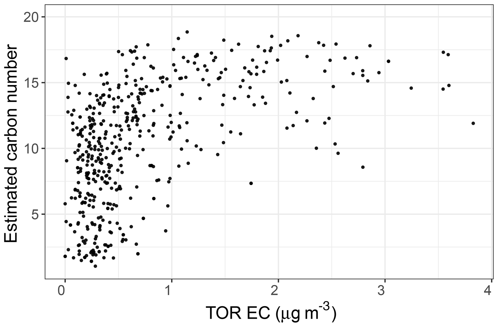
Figure C1Scatter plot showing the relationship between collocated measurements of EC concentration and carbon number estimates by PLSR models in the IMPROVE network in 2011 and 2013.
The baseline-corrected and normalized aliphatic CH peaks of laboratory standards and atmospheric samples are available at https://doi.org/10.5281/zenodo.4882120 (Yazdani et al., 2021).
The supplement related to this article is available online at: https://doi.org/10.5194/amt-14-4805-2021-supplement.
AY and ST conceived of the project. AY prepared laboratory standards, performed the calibrations, and analyzed results. AY wrote the manuscript; ST and AMD provided regular input on the analysis and further editing of the manuscript. AMD provided laboratory and the ambient sample spectra, and ST provided overall supervision of the project.
The authors declare that they have no conflict of interest.
The authors acknowledge funding from the Swiss National Science Foundation (200021_172923) and the IMPROVE program (National Park Service cooperative agreement P11AC91045).
This research has been supported by the Schweizerischer Nationalfonds zur Förderung der Wissenschaftlichen Forschung (grant no. 200021_172923) and the National Park Service (grant no. P11AC91045).
This paper was edited by Paolo Laj and reviewed by two anonymous referees.
Aiken, A. C., DeCarlo, P. F., Kroll, J. H., Worsnop, D. R., Huffman, J. A., Docherty, K. S., Ulbrich, I. M., Mohr, C., Kimmel, J. R., Sueper, D., Sun, Y., Zhang, Q., Trimborn, A., Northway, M., Ziemann, P. J., Canagaratna, M. R., Onasch, T. B., Alfarra, M. R., Prevot, A. S. H., Dommen, J., Duplissy, J., Metzger, A., Baltensperger, U., and Jimenez, J. L.: O/C and OM/OC Ratios of Primary, Secondary, and Ambient Organic Aerosols with High-Resolution Time-of-Flight Aerosol Mass Spectrometry, Environ. Sci. Technol., 42, 4478–4485, https://doi.org/10.1021/es703009q, 2008. a
Atkins, P., de Paula, J., and Keeler, J.: Atkins' Physical Chemistry, Oxford University Press, Oxford, New York, 11th Edn., 2017. a
Boris, A. J., Takahama, S., Weakley, A. T., Debus, B. M., Fredrickson, C. D., Esparza-Sanchez, M., Burki, C., Reggente, M., Shaw, S. L., Edgerton, E. S., and Dillner, A. M.: Quantifying organic matter and functional groups in particulate matter filter samples from the southeastern United States – Part 1: Methods, Atmos. Meas. Tech., 12, 5391–5415, https://doi.org/10.5194/amt-12-5391-2019, 2019. a, b
Breiman, L., Friedman, J. H., Olshen, R. A., and Stone, C. J.: Classification and Regression Trees, Biometrics, 40, 874–874, https://doi.org/10.2307/2530946, 1983. a
Bürki, C., Reggente, M., Dillner, A. M., Hand, J. L., Shaw, S. L., and Takahama, S.: Analysis of functional groups in atmospheric aerosols by infrared spectroscopy: method development for probabilistic modeling of organic carbon and organic matter concentrations, Atmos. Meas. Tech., 13, 1517–1538, https://doi.org/10.5194/amt-13-1517-2020, 2020. a, b, c, d, e, f, g, h, i, j
Canagaratna, M. R., Jayne, J. T., Jimenez, J. L., Allan, J. D., Alfarra, M. R., Zhang, Q., Onasch, T. B., Drewnick, F., Coe, H., Middlebrook, A., Delia, A., Williams, L. R., Trimborn, A. M., Northway, M. J., DeCarlo, P. F., Kolb, C. E., Davidovits, P., and Worsnop, D. R.: Chemical and Microphysical Characterization of Ambient Aerosols with the Aerodyne Aerosol Mass Spectrometer, Mass Spectrom. Rev., 26, 185–222, https://doi.org/10.1002/mas.20115, 2007. a
Cocker III, D. R., Mader, B. T., Kalberer, M., Flagan, R. C., and Seinfeld, J. H.: The Effect of Water on Gas-Particle Partitioning of Secondary Organic Aerosol: II. m-Xylene and 1,3,5-Trimethylbenzene Photooxidation Systems, Atmos. Environ., 35, 6073–6085, https://doi.org/10.1016/S1352-2310(01)00405-8, 2001. a
Corsetti, S., Rabl, T., McGloin, D., and Kiefer, J.: Intermediate Phases during Solid to Liquid Transitions in Long-Chain n-Alkanes, Phys. Chem. Chem. Phys., 19, 13941–13950, https://doi.org/10.1039/C7CP01468F, 2017. a, b
Coury, C. and Dillner, A. M.: A Method to Quantify Organic Functional Groups and Inorganic Compounds in Ambient Aerosols Using Attenuated Total Reflectance FTIR Spectroscopy and Multivariate Chemometric Techniques, Atmos. Environ., 42, 5923–5932, https://doi.org/10.1016/j.atmosenv.2008.03.026, 2008. a
Decesari, S., Facchini, M. C., Fuzzi, S., and Tagliavini, E.: Characterization of Water-Soluble Organic Compounds in Atmospheric Aerosol: A New Approach, J. Geophys. Res.-Atmos., 105, 1481–1489, https://doi.org/10.1029/1999JD900950, 2000. a
DeRieux, W.-S. W., Li, Y., Lin, P., Laskin, J., Laskin, A., Bertram, A. K., Nizkorodov, S. A., and Shiraiwa, M.: Predicting the glass transition temperature and viscosity of secondary organic material using molecular composition, Atmos. Chem. Phys., 18, 6331–6351, https://doi.org/10.5194/acp-18-6331-2018, 2018. a
Desiraju, G. R. and Steiner, T.: The Weak Hydrogen Bond: In Structural Chemistry and Biology, Oxford University Press, 2001. a
Donahue, N. M., Epstein, S. A., Pandis, S. N., and Robinson, A. L.: A two-dimensional volatility basis set: 1. organic-aerosol mixing thermodynamics, Atmos. Chem. Phys., 11, 3303–3318, https://doi.org/10.5194/acp-11-3303-2011, 2011. a, b
Faber, P., Drewnick, F., Bierl, R., and Borrmann, S.: Complementary Online Aerosol Mass Spectrometry and Offline FT-IR Spectroscopy Measurements: Prospects and Challenges for the Analysis of Anthropogenic Aerosol Particle Emissions, Atmos. Environ., 166, 92–98, https://doi.org/10.1016/j.atmosenv.2017.07.014, 2017. a
Fornaro, T., Burini, D., Biczysko, M., and Barone, V.: Hydrogen-Bonding Effects on Infrared Spectra from Anharmonic Computations: Uracil–Water Complexes and Uracil Dimers, J. Phys. Chem. A, 119, 4224–4236, https://doi.org/10.1021/acs.jpca.5b01561, 2015. a
Gentner, D. R., Isaacman, G., Worton, D. R., Chan, A. W. H., Dallmann, T. R., Davis, L., Liu, S., Day, D. A., Russell, L. M., Wilson, K. R., Weber, R., Guha, A., Harley, R. A., and Goldstein, A. H.: Elucidating Secondary Organic Aerosol from Diesel and Gasoline Vehicles through Detailed Characterization of Organic Carbon Emissions, P. Natl. Acad. Sci. USA, 109, 18318–18323, https://doi.org/10.1073/pnas.1212272109, 2012. a, b, c, d
Graber, E. R. and Rudich, Y.: Atmospheric HULIS: How humic-like are they? A comprehensive and critical review, Atmos. Chem. Phys., 6, 729–753, https://doi.org/10.5194/acp-6-729-2006, 2006. a, b
Hähner, G., Zwahlen, M., and Caseri, W.: Chain-Length Dependence of the Conformational Order in Self-Assembled Dialkylammonium Monolayers on Mica Studied with Soft X-Ray Absorption, Langmuir, 21, 1424–1427, https://doi.org/10.1021/la047841u, 2005. a
Hallquist, M., Wenger, J. C., Baltensperger, U., Rudich, Y., Simpson, D., Claeys, M., Dommen, J., Donahue, N. M., George, C., Goldstein, A. H., Hamilton, J. F., Herrmann, H., Hoffmann, T., Iinuma, Y., Jang, M., Jenkin, M. E., Jimenez, J. L., Kiendler-Scharr, A., Maenhaut, W., McFiggans, G., Mentel, Th. F., Monod, A., Prévôt, A. S. H., Seinfeld, J. H., Surratt, J. D., Szmigielski, R., and Wildt, J.: The formation, properties and impact of secondary organic aerosol: current and emerging issues, Atmos. Chem. Phys., 9, 5155–5236, https://doi.org/10.5194/acp-9-5155-2009, 2009. a, b, c, d
Hand, J. L., Prenni, A. J., Schichtel, B. A., Malm, W. C., and Chow, J. C.: Trends in Remote PM2.5 Residual Mass across the United States: Implications for Aerosol Mass Reconstruction in the IMPROVE Network, Atmos. Environ., 203, 141–152, https://doi.org/10.1016/j.atmosenv.2019.01.049, 2019. a, b
Hastie, T., Tibshirani, R., and Friedman, J.: The Elements of Statistical Learning: Data Mining, Inference, and Prediction, Second Edition, Springer Series in Statistics, Springer-Verlag, New York, 2nd Edn., 2009. a
Hastings, S. H., Watson, A. T., Williams, R. B., and Anderson, J. A.: Determination of Hydrocarbon Functional Groups by Infrared Spectroscopy, Anal. Chem., 24, 612–618, https://doi.org/10.1021/ac60064a002, 1952. a
Hawkins, L. N. and Russell, L. M.: Oxidation of Ketone Groups in Transported Biomass Burning Aerosol from the 2008 Northern California Lightning Series Fires, Atmos. Environ., 44, 4142–4154, https://doi.org/10.1016/j.atmosenv.2010.07.036, 2010. a
Hermans, J., Ongay, S., Markov, V., and Bischoff, R.: Physicochemical Parameters Affecting the Electrospray Ionization Efficiency of Amino Acids after Acylation, Anal. Chem., 89, 9159–9166, https://doi.org/10.1021/acs.analchem.7b01899, 2017. a
Iyer, S., Lopez-Hilfiker, F., Lee, B. H., Thornton, J. A., and Kurtén, T.: Modeling the Detection of Organic and Inorganic Compounds Using Iodide-Based Chemical Ionization, J. Phys. Chem. A, 120, 576–587, https://doi.org/10.1021/acs.jpca.5b09837, 2016. a
Jang, M. and Kamens, R. M.: Atmospheric Secondary Aerosol Formation by Heterogeneous Reactions of Aldehydes in the Presence of a Sulfuric Acid Aerosol Catalyst, Environ. Sci. Technol., 35, 4758–4766, https://doi.org/10.1021/es010790s, 2001a. a
Jang, M. and Kamens, R. M.: Characterization of Secondary Aerosol from the Photooxidation of Toluene in the Presence of NOx and 1-Propene, Environ. Sci. Technol., 35, 3626–3639, https://doi.org/10.1021/es010676, 2001b. a
Jathar, S. H., Cappa, C. D., Wexler, A. S., Seinfeld, J. H., and Kleeman, M. J.: Multi-generational oxidation model to simulate secondary organic aerosol in a 3-D air quality model, Geosci. Model Dev., 8, 2553–2567, https://doi.org/10.5194/gmd-8-2553-2015, 2015. a, b, c, d, e, f
Jimenez, J. L., Canagaratna, M. R., Donahue, N. M., Prevot, A. S. H., Zhang, Q., Kroll, J. H., DeCarlo, P. F., Allan, J. D., Coe, H., Ng, N. L., Aiken, A. C., Docherty, K. S., Ulbrich, I. M., Grieshop, A. P., Robinson, A. L., Duplissy, J., Smith, J. D., Wilson, K. R., Lanz, V. A., Hueglin, C., Sun, Y. L., Tian, J., Laaksonen, A., Raatikainen, T., Rautiainen, J., Vaattovaara, P., Ehn, M., Kulmala, M., Tomlinson, J. M., Collins, D. R., Cubison, M. J., E, Dunlea, J., Huffman, J. A., Onasch, T. B., Alfarra, M. R., Williams, P. I., Bower, K., Kondo, Y., Schneider, J., Drewnick, F., Borrmann, S., Weimer, S., Demerjian, K., Salcedo, D., Cottrell, L., Griffin, R., Takami, A., Miyoshi, T., Hatakeyama, S., Shimono, A., Sun, J. Y., Zhang, Y. M., Dzepina, K., Kimmel, J. R., Sueper, D., Jayne, J. T., Herndon, S. C., Trimborn, A. M., Williams, L. R., Wood, E. C., Middlebrook, A. M., Kolb, C. E., Baltensperger, U., and Worsnop, D. R.: Evolution of Organic Aerosols in the Atmosphere, Science, 326, 1525–1529, https://doi.org/10.1126/science.1180353, 2009. a
Kalberer, M.: Identification of Polymers as Major Components of Atmospheric Organic Aerosols, Science, 303, 1659–1662, https://doi.org/10.1126/science.1092185, 2004. a, b
Kalberer, M., Sax, M., and Samburova, V.: Molecular Size Evolution of Oligomers in Organic Aerosols Collected in Urban Atmospheres and Generated in a Smog Chamber, Environ. Sci. Technol., 40, 5917–5922, https://doi.org/10.1021/es0525760, 2006. a, b
Kanakidou, M., Seinfeld, J. H., Pandis, S. N., Barnes, I., Dentener, F. J., Facchini, M. C., Van Dingenen, R., Ervens, B., Nenes, A., Nielsen, C. J., Swietlicki, E., Putaud, J. P., Balkanski, Y., Fuzzi, S., Horth, J., Moortgat, G. K., Winterhalter, R., Myhre, C. E. L., Tsigaridis, K., Vignati, E., Stephanou, E. G., and Wilson, J.: Organic aerosol and global climate modelling: a review, Atmos. Chem. Phys., 5, 1053–1123, https://doi.org/10.5194/acp-5-1053-2005, 2005. a
Kelly, A. M.: Condensed-Phase Molecular Spectroscopy and Photophysics, John Wiley & Sons, Inc., Hoboken, NJ, 1st Edn., 2013. a, b, c
Kroll, J. H. and Seinfeld, J. H.: Chemistry of Secondary Organic Aerosol: Formation and Evolution of Low-Volatility Organics in the Atmosphere, Atmos. Environ., 42, 3593–3624, https://doi.org/10.1016/j.atmosenv.2008.01.003, 2008. a, b, c
Kroll, J. H., Donahue, N. M., Jimenez, J. L., Kessler, S. H., Canagaratna, M. R., Wilson, K. R., Altieri, K. E., Mazzoleni, L. R., Wozniak, A. S., Bluhm, H., Mysak, E. R., Smith, J. D., Kolb, C. E., and Worsnop, D. R.: Carbon Oxidation State as a Metric for Describing the Chemistry of Atmospheric Organic Aerosol, Nat. Chem., 3, 133–139, https://doi.org/10.1038/nchem.948, 2011. a, b
Kuzmiakova, A., Dillner, A. M., and Takahama, S.: An automated baseline correction protocol for infrared spectra of atmospheric aerosols collected on polytetrafluoroethylene (Teflon) filters, Atmos. Meas. Tech., 9, 2615–2631, https://doi.org/10.5194/amt-9-2615-2016, 2016. a, b, c
Li, X., Han, J., Hopke, P. K., Hu, J., Shu, Q., Chang, Q., and Ying, Q.: Quantifying primary and secondary humic-like substances in urban aerosol based on emission source characterization and a source-oriented air quality model, Atmos. Chem. Phys., 19, 2327–2341, https://doi.org/10.5194/acp-19-2327-2019, 2019. a
Li, Y., Pöschl, U., and Shiraiwa, M.: Molecular corridors and parameterizations of volatility in the chemical evolution of organic aerosols, Atmos. Chem. Phys., 16, 3327–3344, https://doi.org/10.5194/acp-16-3327-2016, 2016. a, b
Li, Y., Day, D. A., Stark, H., Jimenez, J. L., and Shiraiwa, M.: Predictions of the glass transition temperature and viscosity of organic aerosols from volatility distributions, Atmos. Chem. Phys., 20, 8103–8122, https://doi.org/10.5194/acp-20-8103-2020, 2020. a
Lii, J.-H., Chen, K.-H., and Allinger, N. L.: Alcohols, Ethers, Carbohydrates, and Related Compounds Part V. The Bohlmann Torsional Effect, The J. Phys. Chem. A, 108, 3006–3015, https://doi.org/10.1021/jp031063h, 2004. a
Lipp, E. D.: Application of Fourier Self-Deconvolution to the FT-IR Spectra of Polydimethylsiloxane Oligomers for Determining Chain Length, Appl. Spectrosc., 40, 1009–1011, 1986. a
Lopez-Hilfiker, F. D., Pospisilova, V., Huang, W., Kalberer, M., Mohr, C., Stefenelli, G., Thornton, J. A., Baltensperger, U., Prevot, A. S. H., and Slowik, J. G.: An extractive electrospray ionization time-of-flight mass spectrometer (EESI-TOF) for online measurement of atmospheric aerosol particles, Atmos. Meas. Tech., 12, 4867–4886, https://doi.org/10.5194/amt-12-4867-2019, 2019. a
Mayo, D. W., Miller, F. A., and Hannah, R. W.: Course Notes on the Interpretation of Infrared and Raman Spectra, John Wiley & Sons, Hoboken, NJ, 2004. a, b, c, d, e
Mcclenny, W. A., Childers, J. W., Rōhl, R., and Palmer, R. A.: FTIR Transmission Spectrometry for the Nondestructive Determination of Ammonium and Sulfate in Ambient Aerosols Collected on Teflon Filters, Atmos. Environ. (1967), 19, 1891–1898, https://doi.org/10.1016/0004-6981(85)90014-9, 1985. a
McHale, J. L.: Molecular Spectroscopy, CRC Press, Boca Raton, FL, 2017. a
Murphy, B. N., Donahue, N. M., Fountoukis, C., Dall'Osto, M., O'Dowd, C., Kiendler-Scharr, A., and Pandis, S. N.: Functionalization and fragmentation during ambient organic aerosol aging: application of the 2-D volatility basis set to field studies, Atmos. Chem. Phys., 12, 10797–10816, https://doi.org/10.5194/acp-12-10797-2012, 2012. a, b
Nozière, B., Kalberer, M., Claeys, M., Allan, J., D'Anna, B., Decesari, S., Finessi, E., Glasius, M., Grgić, I., Hamilton, J. F., Hoffmann, T., Iinuma, Y., Jaoui, M., Kahnt, A., Kampf, C. J., Kourtchev, I., Maenhaut, W., Marsden, N., Saarikoski, S., Schnelle-Kreis, J., Surratt, J. D., Szidat, S., Szmigielski, R., and Wisthaler, A.: The Molecular Identification of Organic Compounds in the Atmosphere: State of the Art and Challenges, Chem. Rev., 115, 3919–3983, https://doi.org/10.1021/cr5003485, 2015. a
Orendorff, C. J., Ducey, M. W., and Pemberton, J. E.: Quantitative Correlation of Raman Spectral Indicators in Determining Conformational Order in Alkyl Chains, J. Phys. Chem. A, 106, 6991–6998, https://doi.org/10.1021/jp014311n, 2002. a
Orthous-Daunay, F. R., Quirico, E., Beck, P., Brissaud, O., Dartois, E., Pino, T., and Schmitt, B.: Mid-Infrared Study of the Molecular Structure Variability of Insoluble Organic Matter from Primitive Chondrites, Icarus, 223, 534–543, https://doi.org/10.1016/j.icarus.2013.01.003, 2013. a
Pankow, J. F. and Barsanti, K. C.: The Carbon Number-Polarity Grid: A Means to Manage the Complexity of the Mix of Organic Compounds When Modeling Atmospheric Organic Particulate Matter, Atmos. Environ., 43, 2829–2835, https://doi.org/10.1016/j.atmosenv.2008.12.050, 2009. a, b
Parks, D. A., Raj, K. V., Berry, C. A., Weakley, A. T., Griffiths, P. R., and Miller, A. L.: Towards a Field-Portable Real-Time Organic and Elemental Carbon Monitor, Mining, Metall. Explor., 36, 765–772, https://doi.org/10.1007/s42461-019-0064-8, 2019. a
Pavia, D. L., Lampman, G. M., Kriz, G. S., and Vyvyan, J. A.: Introduction to Spectroscopy, Brooks Cole, Belmont, CA, 4th Edn., 2008. a, b, c, d, e, f, g
Pope, R., Stanley, K. M., Domsky, I., Yip, F., Nohre, L., and Mirabelli, M. C.: The Relationship of High PM2.5 Days and Subsequent Asthma-Related Hospital Encounters during the Fireplace Season in Phoenix, AZ, 2008–2012, Air Qual. Atmos. Hlth., 10, 161–169, https://doi.org/10.1007/s11869-016-0431-2, 2017. a
Price, D. J., Chen, C.-L., Russell, L. M., Lamjiri, M. A., Betha, R., Sanchez, K., Liu, J., Lee, A. K. Y., and Cocker, D. R.: More Unsaturated, Cooking-Type Hydrocarbon-like Organic Aerosol Particle Emissions from Renewable Diesel Compared to Ultra Low Sulfur Diesel in at-Sea Operations of a Research Vessel, Aerosol Sci. Technol., 51, 135–146, https://doi.org/10.1080/02786826.2016.1238033, 2017. a, b, c
Reggente, M., Dillner, A. M., and Takahama, S.: Predicting ambient aerosol thermal–optical reflectance (TOR) measurements from infrared spectra: extending the predictions to different years and different sites, Atmos. Meas. Tech., 9, 441–454, https://doi.org/10.5194/amt-9-441-2016, 2016. a
Russell, L. M.: Aerosol Organic-Mass-to-Organic-Carbon Ratio Measurements, Environ. Sci. Technol., 37, 2982–2987, https://doi.org/10.1021/es026123w, 2003. a
Russell, L. M., Takahama, S., Liu, S., Hawkins, L. N., Covert, D. S., Quinn, P. K., and Bates, T. S.: Oxygenated Fraction and Mass of Organic Aerosol from Direct Emission and Atmospheric Processing Measured on the R/V Ronald Brown during TEXAQS/GoMACCS 2006, J. Geophys. Res.-Atmos., 114, D00F05, https://doi.org/10.1029/2008JD011275, 2009. a, b
Russell, L. M., Bahadur, R., and Ziemann, P. J.: Identifying Organic Aerosol Sources by Comparing Functional Group Composition in Chamber and Atmospheric Particles, P. Natl. Acad. Sci. USA, 108, 3516–3521, https://doi.org/10.1073/pnas.1006461108, 2011. a
Russo, C., Stanzione, F., Tregrossi, A., and Ciajolo, A.: Infrared Spectroscopy of Some Carbon-Based Materials Relevant in Combustion: Qualitative and Quantitative Analysis of Hydrogen, Carbon, 74, 127–138, https://doi.org/10.1016/j.carbon.2014.03.014, 2014. a
Ruthenburg, T. C., Perlin, P. C., Liu, V., McDade, C. E., and Dillner, A. M.: Determination of Organic Matter and Organic Matter to Organic Carbon Ratios by Infrared Spectroscopy with Application to Selected Sites in the IMPROVE Network, Atmos. Environ., 86, 47–57, https://doi.org/10.1016/j.atmosenv.2013.12.034, 2014. a, b, c, d, e, f, g, h
Seinfeld, J. H. and Pandis, S. N.: Atmospheric Chemistry and Physics: From Air Pollution to Climate Change, John Wiley & Sons, Hoboken, NJ, 2016. a, b
Shiraiwa, M., Berkemeier, T., Schilling-Fahnestock, K. A., Seinfeld, J. H., and Pöschl, U.: Molecular corridors and kinetic regimes in the multiphase chemical evolution of secondary organic aerosol, Atmos. Chem. Phys., 14, 8323–8341, https://doi.org/10.5194/acp-14-8323-2014, 2014. a
Shiraiwa, M., Li, Y., Tsimpidi, A. P., Karydis, V. A., Berkemeier, T., Pandis, S. N., Lelieveld, J., Koop, T., and Pöschl, U.: Global Distribution of Particle Phase State in Atmospheric Secondary Organic Aerosols, Nat. Commun., 8, 15002, https://doi.org/10.1038/ncomms15002, 2017a. a, b, c
Shiraiwa, M., Ueda, K., Pozzer, A., Lammel, G., Kampf, C. J., Fushimi, A., Enami, S., Arangio, A. M., Fröhlich-Nowoisky, J., Fujitani, Y., Furuyama, A., Lakey, P. S. J., Lelieveld, J., Lucas, K., Morino, Y., Pöschl, U., Takahama, S., Takami, A., Tong, H., Weber, B., Yoshino, A., and Sato, K.: Aerosol Health Effects from Molecular to Global Scales, Environ. Sci. Technol., 51, 13545–13567, https://doi.org/10.1021/acs.est.7b04417, 2017b. a
Simon, H., Bhave, P. V., Swall, J. L., Frank, N. H., and Malm, W. C.: Determining the spatial and seasonal variability in OM/OC ratios across the US using multiple regression, Atmos. Chem. Phys., 11, 2933–2949, https://doi.org/10.5194/acp-11-2933-2011, 2011. a, b
Takahama, S., Schwartz, R. E., Russell, L. M., Macdonald, A. M., Sharma, S., and Leaitch, W. R.: Organic functional groups in aerosol particles from burning and non-burning forest emissions at a high-elevation mountain site, Atmos. Chem. Phys., 11, 6367–6386, https://doi.org/10.5194/acp-11-6367-2011, 2011. a
Takahama, S., Johnson, A., and Russell, L. M.: Quantification of Carboxylic and Carbonyl Functional Groups in Organic Aerosol Infrared Absorbance Spectra, Aerosol Sci. Technol., 47, 310–325, https://doi.org/10.1080/02786826.2012.752065, 2013. a, b
Takahama, S., Ruggeri, G., and Dillner, A. M.: Analysis of functional groups in atmospheric aerosols by infrared spectroscopy: sparse methods for statistical selection of relevant absorption bands, Atmos. Meas. Tech., 9, 3429–3454, https://doi.org/10.5194/amt-9-3429-2016, 2016. a
Thomas, M.: Theoretical Modeling of Vibrational Spectra in the Liquid Phase, Ph.D. thesis, Springer International Publishing, Cham, https://doi.org/10.1007/978-3-319-49628-3, 2017. a
Thomas, M., Brehm, M., Fligg, R., Vöhringer, P., and Kirchner, B.: Computing Vibrational Spectra from Ab Initio Molecular Dynamics, Phys. Chem. Chem. Phys., 15, 6608, https://doi.org/10.1039/c3cp44302g, 2013. a
Tolocka, M. P., Jang, M., Ginter, J. M., Cox, F. J., Kamens, R. M., and Johnston, M. V.: Formation of Oligomers in Secondary Organic Aerosol, Environ. Sci. Technol., 38, 1428–1434, https://doi.org/10.1021/es035030r, 2004. a
Trump, E. R. and Donahue, N. M.: Oligomer formation within secondary organic aerosols: equilibrium and dynamic considerations, Atmos. Chem. Phys., 14, 3691–3701, https://doi.org/10.5194/acp-14-3691-2014, 2014. a
Turpin, B. J., Saxena, P., and Andrews, E.: Measuring and Simulating Particulate Organics in the Atmosphere: Problems and Prospects, Atmos. Environ., 34, 2983–3013, https://doi.org/10.1016/S1352-2310(99)00501-4, 2000. a
Wold, S., Martens, H., and Wold, H.: The Multivariate Calibration Problem in Chemistry Solved by the PLS Method, in: Matrix Pencils, edited by Kågström, B. and Ruhe, A., Lect. Notes Math., 286–293, Springer Berlin Heidelberg, 1983. a
Xie, Q., Li, Y., Yue, S., Su, S., Cao, D., Xu, Y., Chen, J., Tong, H., Su, H., Cheng, Y., Zhao, W., Hu, W., Wang, Z., Yang, T., Pan, X., Sun, Y., Wang, Z., Liu, C.-Q., Kawamura, K., Jiang, G., Shiraiwa, M., and Fu, P.: Increase of High Molecular Weight Organosulfate With Intensifying Urban Air Pollution in the Megacity Beijing, J. Geophys. Res.-Atmos., 125, e2019JD032200, https://doi.org/10.1029/2019JD032200, 2020. a
Yazdani, A., Dillner, A. M., and Takahama, S.: Baseline-Corrected Aliphatic CH Peaks in the FTIR Spectra of Laboratory Standards and Atmospheric Aerosols, Zenodo [data set], https://doi.org/10.5281/zenodo.4882120, 2021. a
Yuan, Q., Lai, S., Song, J., Ding, X., Zheng, L., Wang, X., Zhao, Y., Zheng, J., Yue, D., Zhong, L., Niu, X., and Zhang, Y.: Seasonal Cycles of Secondary Organic Aerosol Tracers in Rural Guangzhou, Southern China: The Importance of Atmospheric Oxidants, Environ. Pollut., 240, 884–893, https://doi.org/10.1016/j.envpol.2018.05.009, 2018. a
Zhang, Q., Jimenez, J. L., Canagaratna, M. R., Allan, J. D., Coe, H., Ulbrich, I., Alfarra, M. R., Takami, A., Middlebrook, A. M., Sun, Y. L., Dzepina, K., Dunlea, E., Docherty, K., DeCarlo, P. F., Salcedo, D., Onasch, T., Jayne, J. T., Miyoshi, T., Shimono, A., Hatakeyama, S., Takegawa, N., Kondo, Y., Schneider, J., Drewnick, F., Borrmann, S., Weimer, S., Demerjian, K., Williams, P., Bower, K., Bahreini, R., Cottrell, L., Griffin, R. J., Rautiainen, J., Sun, J. Y., Zhang, Y. M., and Worsnop, D. R.: Ubiquity and Dominance of Oxygenated Species in Organic Aerosols in Anthropogenically-Influenced Northern Hemisphere Midlatitudes, Geophys. Res. Lett., 34, L13801, https://doi.org/10.1029/2007GL029979, 2007. a, b
- Abstract
- Introduction
- Methods
- Results and discussion
- Concluding remarks
- Appendix A: Correlation matrix heat map
- Appendix B: Relating mixture property to pure compound property
- Appendix C: Elemental carbon and carbon number
- Data availability
- Author contributions
- Competing interests
- Acknowledgements
- Financial support
- Review statement
- References
- Supplement