the Creative Commons Attribution 4.0 License.
the Creative Commons Attribution 4.0 License.
 | 14 Jul 2021
W-band radar observations for fog forecast improvement: an analysis of model and forward operator errors
Pauline Martinet
Olivier Caumont
Benoît Vié
Julien Delanoë
Jean-Charles Dupont
Mary Borderies
The development of ground-based cloud radars offers a new capability to continuously monitor fog structure. Retrievals of fog microphysics are key for future process studies, data assimilation, or model evaluation and can be performed using a variational method. Both the one-dimensional variational retrieval method (1D-Var) or direct 3D/4D-Var data assimilation techniques rely on the combination of cloud radar measurements and a background profile weighted by their corresponding uncertainties to obtain the optimal solution for the atmospheric state. In order to prepare for the use of ground-based cloud radar measurements for future applications based on variational approaches, the different sources of uncertainty due to instrumental, background, and forward operator errors need to be properly treated and accounted for.
This paper aims at preparing 1D-Var retrievals by analysing the errors associated with a background profile and a forward operator during fog conditions. For this, the background was provided by a high-resolution numerical weather prediction model and the forward operator by a radar simulator.
Firstly, an instrumental dataset was taken from the SIRTA observatory near Paris, France, for winter 2018–2019 during which 31 fog events were observed. Statistics were calculated comparing cloud radar observations to those simulated. It was found that the accuracy of simulations could be drastically improved by correcting for significant spatio-temporal background errors. This was achieved by implementing a most resembling profile method in which an optimal model background profile is selected from a domain and time window around the observation location and time. After selecting the background profiles with the best agreement with the observations, the standard deviation of innovations (observations–simulations) was found to decrease significantly. Moreover, innovation statistics were found to satisfy the conditions needed for future 1D-Var retrievals (un-biased and normally distributed).
- Article
(1916 KB) - Full-text XML
- BibTeX
- EndNote


The presence of fog is an issue for many modes of transport due to its effect of reducing visibility. When seen at airports, it can mean the grounding of flights, resulting in large economic costs due to delays and cancellations (Gultepe et al., 2007). Reliable fog forecasts, however, can allow for the planning of flights around a fog event, mitigating its impact. The development of high-resolution numerical weather prediction (NWP) models, with horizontal resolutions on the order of 1 km and vertical resolutions on the order of 10 m near the surface, offer the possibility of representing fog events with fine spatial and temporal resolutions. However, fog events are generally still poorly forecast with current NWP models (Steeneveld et al., 2015; Philip et al., 2016).
Fog is defined as the reduction of visibility below 1 km at the surface due to the presence of cloud droplets (American Meteorological Society, 2021) and is thus strictly a boundary layer phenomenon. The lack of accurate observations inside the boundary layer has in recent years become an increasingly discussed subject (NRC, 2009; Hu et al., 2019; Wilczak et al., 2015) and might contribute to the sub-optimal performance of high-resolution NWP models when forecasting boundary layer events, such as fog. Although traditional observation methods, such as radio soundings and in situ surface observations provide the most accurate information, the development of ground-based remote sensing instruments offers measurements with a temporal resolution unmatched by traditional instruments. Thanks to these emerging technologies, new products have been designed that make use of observations from lidars, ceilometers, and visibility meters to aid fog nowcasting, giving fog alerts on an average of 10 to 50 min before fog formation (Haeffelin et al., 2016).
Recent developments in 95 GHz cloud radars have made these instruments much more affordable (Delanoë et al., 2016) allowing for cloud studies, including those on fog processes, to be performed with increased insight (Thies et al., 2010; Dupont et al., 2012; Wærsted et al., 2017). These have highlighted which physical processes are the most important to improve in new models if fog characteristics are to be better represented. The assimilation of cloud radar data into an operational NWP model to give better fog forecasts with longer lead times, however, is yet to be developed.
A simple method for assimilating new observations into an NWP model is to first retrieve an atmospheric profile of a variable or set of variables and to then assimilate this retrieved profile. Retrievals can be made through different methods (e.g. statistical laws or optimal estimations (OEs) (Maahn et al., 2020) using so-called one-dimensional variational (1D-Var) retrievals of state variables (Martinet et al., 2015)). This study focuses on the preparation of future OEs using 1D-Var data assimilation methods such as in the work of Martinet et al. (2015, 2017) for temperature and humidity profiles.
The main goal of this work with respect to future OE retrievals is to use radar reflectivity observations in combination with microwave radiometer (MWR) brightness temperature observations to provide estimations of liquid water content (LWC) in addition to temperature and humidity. As radar reflectivity is also sensitive to the total cloud droplet number concentration and the distribution of the droplets, it may also be possible to add parameters related to this to the set of retrieved variables in an OE algorithm. However, as a one-moment microphysical scheme is currently used in the operational AROME model and due to the added complexity of adding the droplet number concentration number first, 1D data assimilation experiments will focus only on the liquid water content retrieval.
These retrievals may then be used in a second step with a three- or four-dimensional variational data assimilation (3D/4D-Var) scheme (Bauer et al., 2006; Janisková, 2015) or as a preliminary step towards direct variational data assimilation of the cloud radar reflectivity (Fielding and Janiskova, 2020). In order to first perform the 1D-Var retrieval, observations should be combined with an a priori profile, otherwise known as a “background” profile. Though this may be taken from climatological data, the more accurate the background profile, the more accurate the final retrieval is likely to be (Rodgers, 2000). As commonly used in data assimilation, the background profile considered in this study comes from a high-resolution NWP model – in this case the French convective-scale model AROME (Seity et al., 2011), valid at the time and location of the retrieval. In this study, forecast terms (the length of time between the analysis and the predicted phenomena) of 10 to 180 min were used, with a new forecast being issued every 3 h.
In the 1D-Var algorithm, a minimization is performed on the difference between the background profile and observations. This requires variables to be of the same type; in the case of remote sensing instruments this requires either a “backward” model to transform the observation variables into those produced by the NWP model or a “forward” model to transform the variables given by an NWP model to those made by the instrument. Due to the ill-posed nature of transforming radar reflectivity measurements into LWC estimates (Atlas, 1954; Bohren and Huffman, 2008; Maier et al., 2012), the forward model approach has been chosen in this study. The main advantage of using a forward model compared to a backward model, when only cloud droplets as hydrometeors are considered, arises from the ability to easily model attenuation from cloud droplets, water vapour, and dry air in the forward direction.
In order to make a 1D-Var retrieval, it is also necessary that the errors associated with the background and the observations are properly modelled (Rodgers, 2000). For successful variational retrievals to be made, it is assumed that (i) the distribution of errors should follow a normal distribution and (ii) that there should be no systematic bias in the error distributions (Bouttier and Courtier, 2002). Background errors are due to inaccuracies in NWP forecasts. The forward model may contain errors as a result of the hypotheses needed to simulate the observations, such as assumptions on the cloud droplet size distribution in the context of radar reflectivity. Observation errors are due to calibration uncertainties (Toledo et al., 2020; De Angelis et al., 2017), instrumental drifts, and random noise.
The modelling of the errors associated with the background, the observations, and the forward operator can be difficult to specify for a given retrieval, owing to dependencies on the type of weather conditions observed or the forecast term used as a background profile, for example. However, an improved knowledge of background and observation errors is required before the assimilation of any new observation type. The aim of this work is thus to investigate the types of systematic and random errors that may be present in the three sources of errors previously mentioned focusing on newly developed 95 GHz cloud radar during fog conditions.
This study has been performed using a dataset from the SIRTA observation site near Paris (Haeffelin et al., 2005), which hosts a 95 GHz cloud radar, a ground-based microwave radiometer, and other remote sensing and in situ instruments making continuous measurements. Up to 3 h forecasts from the AROME model were used in conjunction with a radar simulator, also referred to as observation operator or forward operator, designed for airborne 95 GHz cloud radar (Borderies et al., 2018).
In this article, an overview of the fog events used in this study is given first. The performance of the AROME model is then analysed using a range of instruments to compare to the observed event. A method is then outlined for the selection of a background profile that is expected to optimize future retrievals. Statistics are then presented showing reflectivity innovations and the improvement gained through the profile selection method.
2.1 SIRTA observatory
All observations for this study were made at SIRTA (Site Instrumental de Recherche par Télédétection Atmosphérique) (Haeffelin et al., 2005). Geographically, the site is located in the suburbs, about 20 km south of Paris, on the campus of the École Polytechnique in Palaiseau, which is a semi-urban environment with trees, fields, houses, and some industrial buildings. The observatory sits on a relatively flat plateau at around 160 m above sea level (a.s.l.). The period between 1 November 2018 and 19 February 2019 was analysed due to the relatively high concentration of fog events seen throughout this period.
2.2 BASTA cloud radar
The cloud radar used in this study is a 95 GHz frequency-modulated continuous wave (FMCW) Doppler radar named the Bistatic Radar System for Atmospheric Sounding (BASTA; Delanoë et al., 2016). The instrument is a product of recent developments aimed at producing an inexpensive radar system to be used operationally. For this reason, the normally expensive high-powered pulsed transmitter has been replaced with a continuous transmitter with frequency modulation, to allow for the backscatter power and the line of sight velocity from the targets – in this case cloud droplets – to be determined. The benefit of using a cloud radar with a 95 GHz transmission frequency compared to radars using lower frequencies is in the sensitivity to cloud droplets. Where the Rayleigh approximation is valid, the power of the reflected radiation will be proportional to the sixth power of the radius of a spherical droplet and inversely proportional to the fourth power of the wavelength of incident light. Thus, for a given transmitted power, radars operating at a higher frequency will have a greater sensitivity to smaller droplets. It does mean, however, that when large particles such as rain, hail, or graupel are encountered, the signal can become quickly attenuated (Kollias et al., 2007).
For monostatic radars, the receiver must be switched off during the transmission of a pulse, meaning that signal backscattered close to the radar cannot be detected and a minimum detectable range of over 100 m is typical for cloud radars sounding in a boundary layer mode (Liu et al., 2017). The fact that BASTA has separate receiving and transmitting antennas (bistatic) allows the minimum measurement distance of the radar to be relatively small compared to that of a monostatic radar. It is capable of making measurements as close as 40 m above ground level, though the minimum detectable measurement values are quite high at this distance ( dBZ for BASTA-SIRTA). This is due to the interaction between the antennas of the transmitter and receiver at close distances. The radar operates in three different modes with vertical resolutions ranging from 12.5 to 100 m and maximal measurement distance from 12 to 18 km respectively. For the BASTA-SIRTA, a 3 s integration time is used, and the three different modes are cycled through continuously. This therefore gives observations for each mode once every 9 s.
The uncertainty associated with BASTA measurements will vary with usage and meteorological conditions. From a comparison with radar reflectivity simulations with rain rates over 2 mm h−1, the estimated uncertainty, provided that the radome is not wet, is between 0.5 to 2.0 dB (Delanoë et al., 2016). A wet radome can affect readings by up to 14 dB. Below 230 m, the far field approximation, which is used to give the radar reflectivity value, is not valid. An overlap correction derived using rain events is therefore used to correct for this effect (Delanoë et al., 2016).
2.3 Other instruments
In order to define fog events, the visibility at or near surface height must be known. Though there has been work done to classify the visibility from radar reflectivity (Li, 2015), which was done with a plan position indicator (PPI) scanning strategy, the lowest gates still suffered from quality issues due to ground clutter. The most reliable way to measure the visibility is with a visibility meter. The visibility meter deployed at ground level at SIRTA is the Degreane Horizon DF320 visibility monitor. This is able to give the meteorological optical range from 5 m to 70 km, with a measurement error under 5 km of 10 %.
Ground-based microwave radiometers also provide insight into the fog properties through liquid water path retrievals. The HATPRO microwave radiometer (Rose et al., 2005) operates in two spectral bands (22 to 31 GHz and 51 to 58 GHz) in order to make retrievals of the temperature and humidity profiles, integrated liquid water, and water vapour contents providing information about the atmospheric stability. For this study, only the liquid water path retrievals were used. These retrievals have an expected accuracy of 20 g m−2 (Crewell and Löhnert, 2003).
A ceilometer was used primarily for the classification of fog types. Low cloud whose base is descending is very likely to be observed before an instance of cloud base lowering (CBL) fog. A Vaisala CL-31 ceilometer (Martucci et al., 2010) was used to measure the cloud base height. This uses a pulse lidar to sense the cloud base and is capable of sensing up to three layers simultaneously with a range from 0 to 7.6 km.
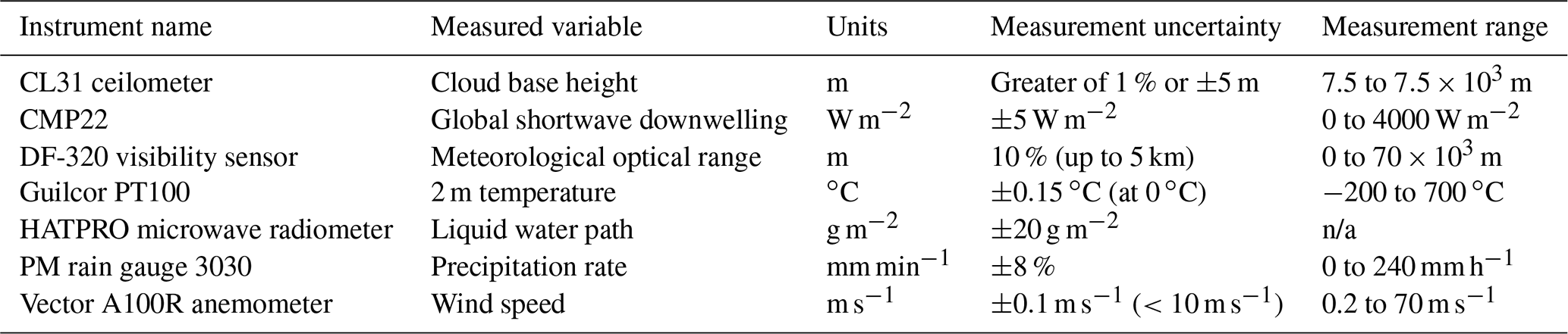
The wind speed, temperature, and rain rate at surface are also important parameters to sense when determining the fog events and classifying them. The specifications for the instruments used in this study are noted in Table 1.
Table 1Instruments used at SIRTA observatory. “n/a” stands for “not applicable”.
2.4 The AROME model
The NWP model used in this study is the French convective-scale model AROME (Seity et al., 2011). AROME has been used operationally since 2008, but has since seen improvements in the horizontal resolution from 2.5 to 1.3 km and in the vertical resolution, which has advanced from 60 to 90 levels, with the first level starting 5 m above the surface. Near the surface, the vertical levels are aligned with the topography and then spaced so as to follow isobars at the top of the model. The model covers a domain centred on France and encompassing most of western Europe. A 3D-Var data assimilation cycle takes place once every hour.
The model was developed from the Meso-NH research model (Lafore et al., 1998; Lac et al., 2018); therefore, most of the model physics is resolved in the same way. A bulk one-moment microphysical scheme is used (ICE-3, Pinty and Jabouille, 1998), which fixes the droplet number concentration over land and sea and specifies six species of atmospheric water (graupel, ice, snow, rain, cloud liquid water over land, and cloud liquid water over sea). An analysis of the parameters used in ICE-3 and their effect on the distribution shape is given in Sect. 4. Table 2 summarizes the parameterization schemes relevant to fog processes with the corresponding references.
Pinty and Jabouille (1998)Mlawer et al. (1997)Fouquart and Bonnel (1980)Masson et al. (2013)Cuxart et al. (2000)Masson (2000)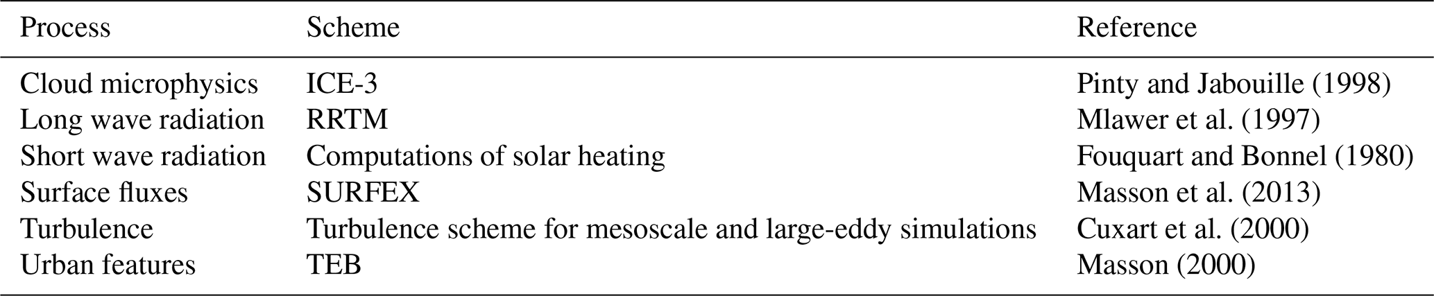
2.5 The forward operator
The forward operator used to convert the parameters supplied by the AROME model into radar reflectivity was developed by Borderies et al. (2018) and designed for vertically pointing airborne W-band cloud radars. Input variables include vertical profiles of pressure, temperature, humidity, and the content of five hydrometeor types (rain, graupel, snow, ice, and liquid cloud). From this, it simulates the reflectivity at the resolution of the input profiles with attenuation taken into account for hydrometeors and moist air. The Liebe (1985) model is used to calculate attenuation by moist air. The reflectivity calculations are consistent with the ICE-3 bulk microphysical scheme, which is operationally used in the AROME model. The sensitivity of the radar is also taken into account by limiting the minimum simulated reflectivity to the minimum observed reflectivity at each range gate.
Two versions of the radar simulator were developed: the one used in this work employs the Mie approximation (Wriedt, 2012), which models particles as spherical and is a valid approximation for cloud liquid water droplets. A version using a T-matrix method is also available for simulating reflectivity from hydrometeors with a more complex shape.
1D-Var retrievals can be highly sensitive to the background profile as demonstrated by Ebell et al. (2017) in the context of LWC retrievals from MWR and 35 GHz cloud radar synergy. Background profiles are commonly provided by short-term forecasts from NWP models, which are prone to errors of different nature, such as temporal and spatial errors. This section aims at a better understanding of typical errors from the AROME background profiles during fog conditions.
3.1 Overview of the observed fog events
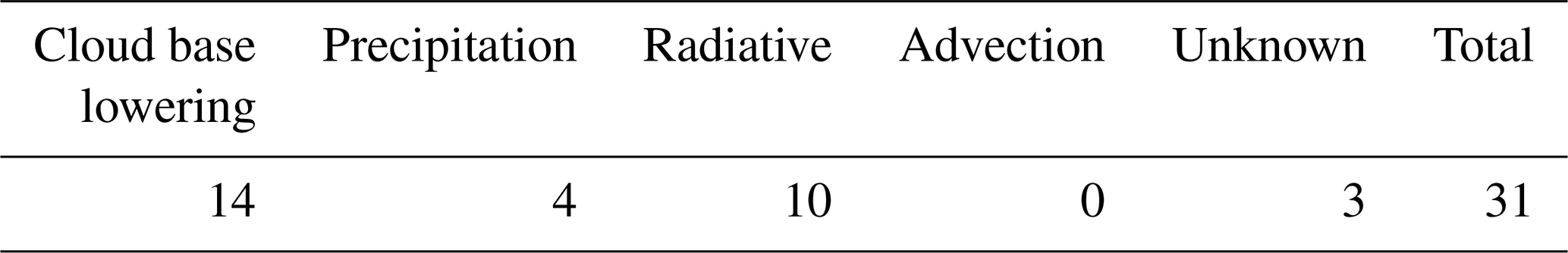
Fog can occur through several atmospheric processes, not all of which are modelled equally well. Philip et al. (2016) have shown that the AROME model seems to succeed in predicting certain types of fog better than others. Notably, CBL events are badly predicted compared to radiative fog. A simple fog classification based on the one described in Tardif and Rasmussen (2007) was performed on the instrumental dataset after updates in the suggested thresholds chosen in the classification. These updates concerned the precision of the conditions and reflected some misleading instrument readings. A total of 31 fog events were observed over the period, and the numbers of each type are detailed in Table 3. In line with previous studies performed by Philip et al. (2016) and Dupont et al. (2016) looking at fog events in Paris and by Román-Cascón et al. (2019) examining fog events over a short period in January 2016 on the Spanish Northern Plateau, the majority of fog events were either cloud base lowering or radiative. Precipitation fog was the third most observed type, for which fog events were typically shorter than radiative or cloud base lowering. The quality of AROME short-term forecasts during these 31 fog events is investigated in the next sections with a focus on spatial and temporal errors as well as typical fog parameters (duration, formation, dissipation times, thickness (or fog top height, here used interchangeably), and liquid water content).
Table 3Number of fog types observed at the SIRTA observation site between 1 November 2018 and 19 February 2019.
3.2 AROME forecast skill scores during fog conditions
In order to make a comparison between observed and modelled fog events, it is necessary to define an equivalent definition of fog events from parameters inside the AROME model. For this study, AROME forecasts were regenerated with outputs produced with a temporal period of 10 min and with forecast terms of 0 to 180 min. The forecasts were extracted for a 28 km × 28 km domain centred on the SIRTA observatory site. Visibility in the AROME model was diagnosed from a newly developed parameterization based on the liquid water content profile according to Dombrowski-Etchevers et al. (2021), which has been used operationally to give a visibility output from the model since July 2019.
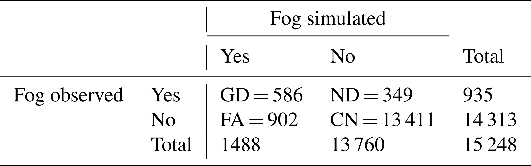
A comparison of observed fog to predicted fog in the model – for the time and grid point corresponding to the time and location of the observation – was carried out. Visibility measurements taken from the DF-320 visibility sensor were averaged over a 10 min period, and where visibility values of lower than 1 km were observed, this was considered as a fog “block”. The same threshold was used with visibility diagnosed from the model to define model fog blocks. As model outputs were available with a temporal resolution of 10 min, these were not averaged. The accuracy of the model was then analysed by comparing each 10 min block in the model against each block from the averaged visibility. Observations where rain was sensed with the rain gauge and simulations in which rain was present in the bottom layer were not considered as fog. The commonly used contingency table based on this comparison is shown in Table 4 where GD indicates cases of good fog detection, FA cases of false alarm, ND cases of fog events missed by the model, and CN correct negatives.
Table 4Contingency table of fog profiles seen in the simulation and observations. Good detection (GD) occurs at the intersection of fog simulated and observed, false alarm (FA) is where fog is simulated but not observed, unpredicted (ND) is where fog is observed but not simulated, and correct negative (CN) is where fog is neither predicted nor observed.
Based on this table, the frequency bias index (FBI), which assesses the over- or under-prediction of an event, and critical success index (CSI), which assesses how well events are forecast, are calculated. These indices are defined in Eqs. (1) and (2). FBI scores can range from 0 to infinity, where a perfect score is 1, and less than 1 indicates an under-prediction of events and greater than 1 indicates an over-prediction. CSI scores can range from 0 to 1, with the perfect score being 1. The probability of detection (POD), the probability of an observed event being forecast, and the false alarm ratio (FAR), which is the probability of a fog forecast being incorrect, are also given Eqs. (3) and (4).
FBI and CSI scores were found to be 1.59 and 0.32 respectively. The scores agree well with the work of Philip et al. (2016) who calculated a score of 1.24 and 0.37 respectively as well as Martinet et al. (2020) who found scores of 1.77 and 0.35. The FBI score indicates that the model over-predicts the occurrence of fog with a large number of false alarms and the CSI score means that 32 % of events observed and/or predicted are correctly forecast by the model. As the CSI “assumes that the times when an event was neither expected nor observed are of no consequence” (Schaefer, 1990), this can be a useful metric to consider. The POD is 63 %, meaning that background profiles of acceptable quality could be expected to be found at about this rate without any other selection method during fog events. With a 60 % FAR, this also highlights how large errors are made when the closest AROME grid point (both spatially and temporally) is used during a fog-clear scene. The next section investigates how much spatio-temporal variability affects fog forecast errors in the AROME model.
3.3 Spatial and temporal error analysis
Spatial and temporal errors refer to modelled fog events that are spatially and/or temporally displaced from the true event. These types of errors were examined to quantify how they can affect the forecast scores.
Firstly, spatial errors were examined by looking at the thickness of the fog layer over the 28 km × 28 km domain around the observation. The fog thickness was diagnosed from simulated reflectivity values and is explained in more detail in Sect. 3.4. Figure 1 shows an example of the development of a radiative fog event on 4 November 2018, which persisted for around 8 h in the model and around 5 h in the observations. The surface height is shown in black contours on the figures, with the higher surfaces in the top left of the map. In the formation stage of the event, approximately half of the domain is covered by fog. The differences in fog thickness at this stage of the event are around 100 m for the AROME grid points already covered by fog. At 05:00 UTC, in the mature phase of the event, the fog thicknesses have approximately the same variability as in the early formation stage, but almost all of the AROME grid points have fog conditions. It may also be noted that the thickest fog layers occur where surface height is the lowest, showing how fog top heights are related to the topography – a subject that is beyond the scope of this work and has been widely discussed elsewhere (Müller et al., 2010; Ducongé et al., 2019). At 10:20 UTC, shortly before the fog event ends, there is substantial variability of around 150 m and in several AROME grid points the event has already dissipated. After 11:00 UTC, the fog layer lifts and disperses and the modelled fog event ends throughout the whole domain.
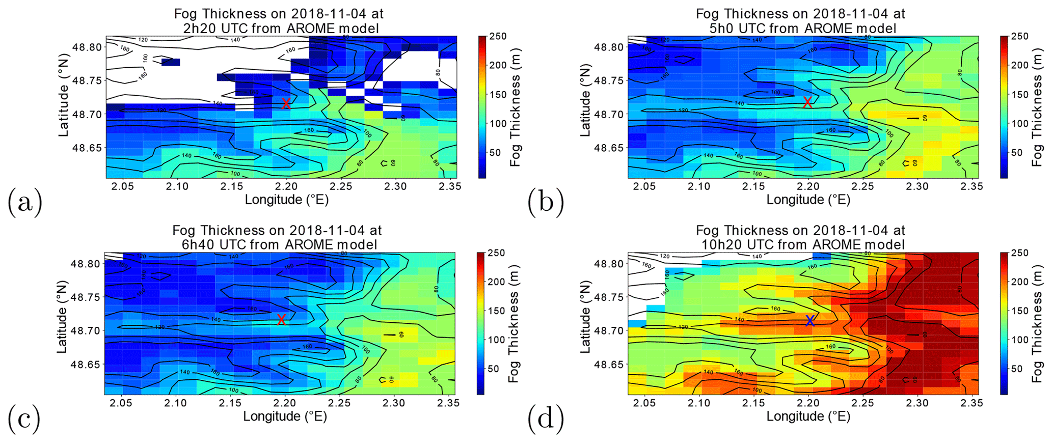
Figure 1Fog top altitude above ground level in the AROME model during a radiative fog event (a) in the formation phase of the event at 02:20 UTC, (b) in the mature phase at 05:00 UTC, (c) in the mature phase at 06:40 UTC, and (d) in the dissipation phase at 10:20 UTC. The fog event ended at around 11:30 UTC in the model. The SIRTA site is marked by the red or blue cross. Black contours represent the surface height.
The significant variability in simulated fog thickness indicates that during the formation and dissipation phases of the fog event, increased value may be brought to the background accuracy by choosing a model profile that more closely fits the observed atmospheric profile than the closest grid point. Figure 2 shows the observed and simulated radar reflectivity profiles for the case on 4 November 2018 for two instances of fog recorded in the observations and fog predicted by the simulation. In both cases, the model overestimates the fog thickness; however, this overestimation is lower in the mature phase compared to the dissipation phase (30 m vs. 80 m).
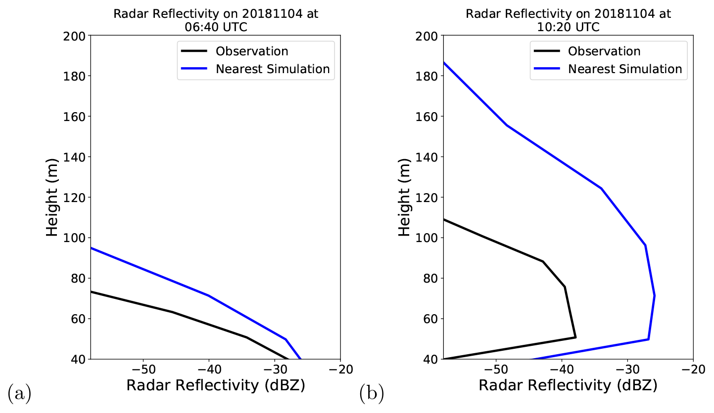
Figure 2Observed and simulated radar reflectivity from the radiative fog event during the mature phase (a) and dissipation phase (b). The black line shows the radar reflectivity measured with the BASTA cloud radar situated at SIRTA. The blue line shows the simulated radar reflectivity from the AROME model forecast, valid at the same time and grid point as the observation.
The temporal errors associated with fog forecasts were then examined. For each observed fog event, the corresponding starting and ending time in the model space was found by looking over a 12 h window (±6 h) around the observation. If two events were seen in the model within one observed event, the closest start and end times corresponding to the observations were taken. Out of 31 fog events observed, 21 could be matched within the 12 h window to a simulated event meaning that 10 observed events could not be matched to a modelled event. The histograms in Fig. 3 show the distribution of hours for which fog was observed and simulated and the temporal differences in the formation time, dissipation time, and duration of fog events observed. The diurnal cycle of fog events is generally well predicted by the model, with the majority of events taking place between midnight and late morning time. It may be seen with formation and dissipation time differences that most fog events that occur in both the observations and simulations have start and end time differences of less than 3 h. The simulated events tend to form earlier (with a median of 25 min) and dissipate later (with a median of 20 min) than the observed events. When all fog events observed and modelled are considered, modelled fog events tend to have a shorter duration, with an average fog time length of 4 h 53 min (4H53M) compared to 6H03M for observed events, as many more short fog events were present in the model but not in the observations than vice versa. When only fog events present in the model and observation were compared, the mean duration of the modelled events was longer (6H44M for modelled events compared to 6H12M for observed events).

Figure 3(a)–(d) Times at which fog was observed (brown bars) and predicted by AROME model (red bars); duration of fog events observed and predicted by the model; fog formation time differences for matching events; fog dissipation time differences for matching events (differences are positive where fog forms or dissipates later in the observation).
It was found that the rate of formation between 10:00 and 20:00 UTC (not shown in Fig. 3) was larger in the observations than in the model, whilst between 00:00 and 8:00 UTC the model had a greater susceptibility to predict fog formation. This result indicates that the model over-predicts the rate of night fog and under-predicts the rate of afternoon fog, which could indicate that the radiation budget of the model could be improved.
3.4 Fog property error analysis
In addition to spatial and temporal errors, the AROME background accuracy will depend on the capability of the AROME model to reproduce the vertical structure of fog microphysical properties. A radar–microwave radiometer combination enables the measurement of fog characteristics such as the layer thickness and the liquid water path of the fog layer. Analysis of a high-resolution model's accuracy in predicting these variables has not been extensively carried out in previous work, as without these instruments a labour intensive method involving tethered balloons or unmanned aerial vehicles (UAVs) is required. The fog layer thickness depends on the rate of cooling, the entrainment, and surface interactions among other processes. It was also demonstrated by Wærsted (2018) that the fog top height is a key parameter in determining the fog dissipation. It thus follows that the better the fog top height prediction, the better the fog dissipation forecast will be. This section aims at investigating fog thickness and liquid water path (LWP) errors observed in the AROME fog forecasts during the winter 2018–2019.
Fog thicknesses were derived from the radar observations during fog conditions. This was found from the height at which the radar reflectivity dropped below the larger of −45 dBZ or the sensitivity of the radar (whichever value was greater) at that range gate. The fog top height was then found in the model from the simulated reflectivity (with the same conditions) for times when fog conditions were simulated. The height resolution of the radar was 12.5 m, whereas the resolution for the model ranged between 12 m at the surface to 65 m at 750 m a.g.l., giving an uncertainty in fog top height difference of 12.25 to 37.75 m. Comparisons were made between the two for times when both observations and simulations are under fog conditions. Figure 4 shows the distribution of fog top height differences where a positive thickness difference means an observed fog top higher than the simulated fog top. The figure shows that errors of up to 300 m were found and 44 % of fog top height differences were greater than 100 m. The mean height difference is −22.5 m and the standard deviation of fog top heights is 104 m.
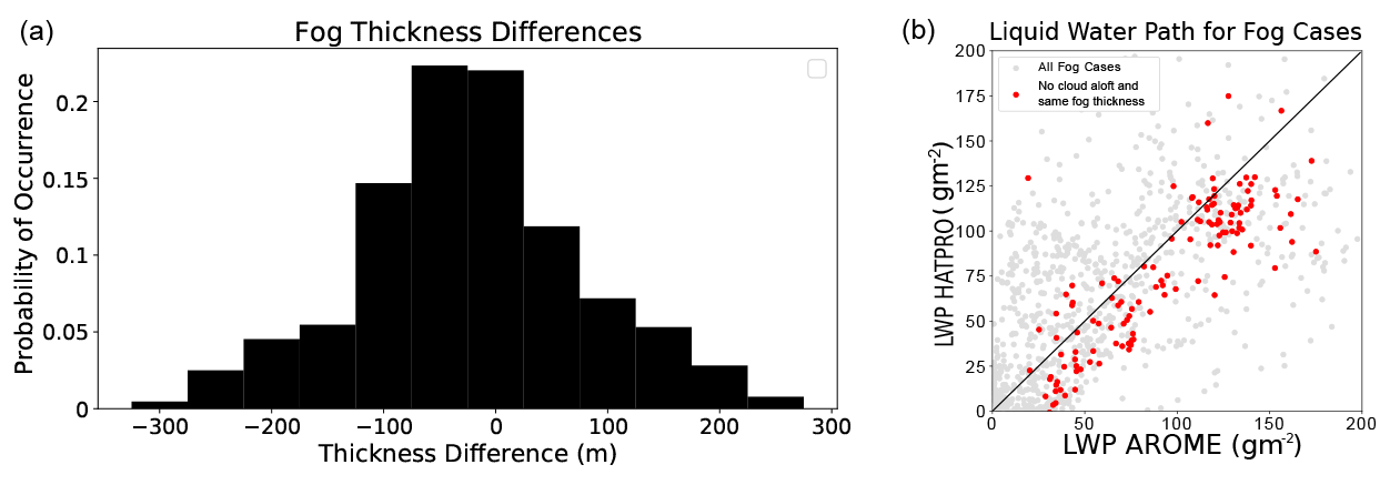
Figure 4(a) Histogram of differences in the fog top height observed with the cloud radar and simulated by the AROME model (observation–simulation) when fog is both observed and simulated. Positive differences represent a larger observed fog thickness than is simulated. (b) Liquid water path recorded on the microwave radiometer and predicted in the AROME model for times at which both predict fog presence. All cases of fog in both the model and observations without restrictions are shown in grey. Red points show LWP values where the integrated cloud thickness above the fog layer does not exceed 25 m (in either the model or observations) and the difference between the model and the observation fog top is less than 25 m.
As liquid water content is the variable responsible for causing fog, its accuracy will thus determine the quality of fog forecasts. As there are no in situ sensors for recording the liquid water content at the observation site, the integrated value of the liquid water path (LWP) from the HATPRO microwave radiometer was used to evaluate the quality of the liquid water content forecast in the model. By comparing liquid water paths for all fog cases, we are left open to comparing not only the error in the thickness and density of the fog layer, but also of clouds aloft. Data from the radar were therefore used to select cases of fog during which the layers of cloud aloft were less than 25 m thick. Similarly, cases where the model simulates thick clouds aloft were discarded. The liquid water path was then compared for cases where the thickness of the fog layer predicted in the model and observed had differences of less than 25 m (Fig. 4). As expected, the differences in liquid water path decrease with the constraints. For cases where there is simply fog observed and simulated, the bias in LWP is 8 g m−2 of over-prediction by the model and a standard deviation of 66 g m−2. For the model–observation comparisons where the fog thicknesses are the same and no cloud aloft is seen, there is a bias of 14 g m−2 of over-prediction in the model and a standard deviation of 26.4 g m−2. As is also shown in Fig. 4, the model more frequently over-predicts the fog thickness than under-predicts it, accounting for the positive LWP bias. Given the accuracy of the liquid water path retrieved from the microwave radiometer of approximately 20 g m−2, as outlined in Sect. 2.4, it can be concluded that when the fog layer thickness is well predicted by the AROME model, the liquid water content inside the fog layer is also well predicted.
From the analysis presented in this section, it may be concluded that significant variations both temporally and spatially could provide scope for the selection of a background profile, which does not correspond directly to the location and time the observation was made. The analysis of the liquid water content prediction of the model, however, shows that the model can be reliable providing that fog is forecast with a similar thickness to that observed. In the next section, the forward operator is evaluated for sources of error, and then comparisons are made between observed cloud radar profiles and profiles simulated from the AROME model. A methodology is also proposed for selecting a background profile that better corresponds to the observed profile.
4.1 Forward operator sensitivity study
The radar simulator was based on radar equations that link the hydrometeor contents contained within a parcel of air to the recorded reflectivity. The attenuation and the reflectivity values both depend on the size and number of droplets. As there is a very large number of ways a mass of water could theoretically be divided among droplets, a size distribution needs to be assumed based on observed droplet size distributions. The droplet size distribution used in this work is consistent with the one used in the AROME model, the one-moment microphysical scheme ICE-3. This uses a modified gamma distribution, as specified in Eqs. (5) and (6).
In the set of equations, N(D) is the droplet number concentration where D is the droplet diameter. Coefficients a and b determine the mass–diameter relationship of the droplets (Eq. 7), which when applied to cloud droplets are well known due to their spherical nature and are set at 524 kg m−b and 3 respectively. α and ν are fixed coefficients, referred to as the shape parameters and are set to 1 and 3 respectively in ICE-3 for cloud liquid droplets over land. N0 is the total droplet number concentration and is set to 300 cm−3 in ICE-3 for liquid cloud over land. M is the liquid water content of the grid point in kg m−3.
The advantages of using this modified gamma distribution are that the shape and median diameter of the distribution are modified with the liquid water content and number concentration of the cloud. For example, when using the modified gamma distribution with a total concentration of 30 cm−3, the median diameter will be greater than for a total concentration of 300 cm−3, as illustrated in Fig. 5.

Figure 5Modified gamma distributions for a liquid water content of 0.12 g m−3 prescribed by the ICE-3 scheme. From (a): α=1 and α=3 (default = 1), ν=2.5 and ν=15 (default = 3), and N=30 cm−3 and N=300 cm−3 (default = 300 cm−3).
As all parameters of the modified gamma distribution except for the liquid water content are held constant in ICE-3, when radar simulations are made for cloud with a droplet size distribution that the parameters do not accurately describe, errors are likely to be made in the calculation of radar reflectivity. In order to assess this uncertainty, simulations were made on an AROME model profile in fog conditions for which the size distribution parameters were perturbed. These perturbations would need to reflect potential variabilities seen in (continental liquid water) fog and low liquid cloud.
Microphysical observations have been investigated on fog events in previous work (Mazoyer et al., 2019; Podzimek, 1997), which tend to show lower droplet number concentrations than is prescribed for continental clouds in the ICE-3 microphysical scheme (of 300 cm−3). From the work of Mazoyer (2016), which looked at median droplet concentrations for continental fog events, and Zhao et al. (2019), which investigated the microphysics of continental boundary layer clouds, reasonable lower and upper bounds of the N0 parameter of 30 and 300 cm−3 were chosen. Figure 5 shows the difference in cloud droplet distribution shapes when these two values are used.
As the α and ν parameters both affect the width of the size distribution (as seen in Fig. 5), it has been a common approach (Mazoyer, 2016; Geoffroy et al., 2010) to fix α and to optimize the value of ν. The most frequently used values are α=1 (Liu and Daum, 2000) and α=3 (Seifert and Beheng, 2001). For this work, it was decided to use α=1, which was shown by Mazoyer (2016) to best represent fog droplet size distributions and also for consistency with the ICE-3 value.
From previous studies examining the value of ν where α=1 (Geoffroy et al., 2010; Miles et al., 2000) it was decided that a range of ν=6.8 to 11.1 should be used. The modified gamma distribution with these values is shown in Fig. 5. Though there may be correlations between the LWC and the value of N and ν, a parameterization for the values of ν and N0 for fog in the context of cloud radar has yet to be performed. For this reason, the parameters ν and N0 are treated as varying randomly for the purpose of investigating the uncertainty in simulated reflectivity.
It can be seen from Fig. 5 that the effect of increasing the ν parameter was a narrowing of the distribution, meaning fewer droplets at the smaller and larger end of the spectrum. The concentration of the largest droplet sizes (above 35 µm) is therefore reduced through these changes. As the radar reflectivity is proportional to the sixth moment of the droplet size where the Rayleigh approximation is valid, this causes smaller values of reflectivity to be simulated. The perturbations in number concentration, meanwhile, were almost entirely below the value in ICE-3, with a range of 30 to 300 cm−3 compared to a value of 300 cm−3 in ICE-3. As seen in Fig. 5, this caused an increase in the number of large droplets (over 50 µm and thus an increase in the simulated reflectivity).
In order to assess the uncertainty in the simulations resulting from the uncertainty in the size distribution parameters ν and N0, simulations were made by perturbing these parameters according to the typical uncertainties from the literature previously discussed. An atmospheric profile under fog conditions was selected from the AROME model with a maximum LWC of 0.12 g m−3 at 71 m a.g.l. Reflectivity was then simulated with changes to the default parameters of the modified gamma distribution. Firstly, the number concentration was held constant whilst perturbations were made to the ν parameter. The same process was repeated keeping value of ν constant and simulating the reflectivity with perturbations in the N0. The obtained distribution of reflectivity values is shown in Fig. 6.
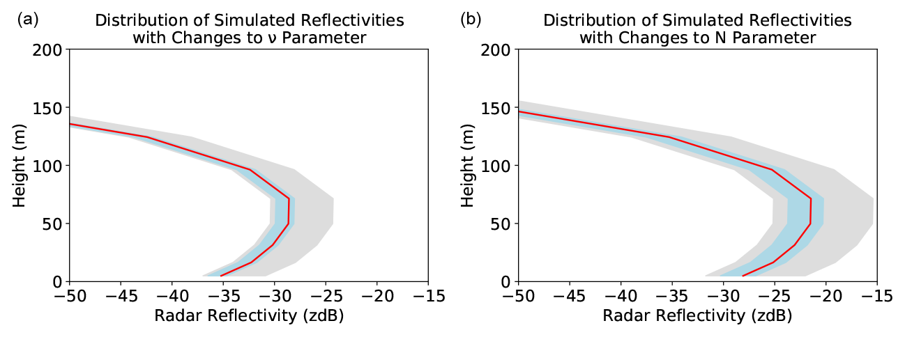
Figure 6Spread of simulated values of radar reflectivity with height for a change in the microphysical parameters of a modified gamma distribution ν (a) and number concentration (b) for a fog profile. The 25th and 75th percentiles are shown in blue, and the median reflectivity shown by the red line.
It can be seen that the uncertainty in the number concentration contributes the most to the uncertainty in the simulated reflectivity. For the altitude at which the liquid water content is the largest, at 0.12 g m−3, the reflectivity difference reaches 9.5 dB between the highest and lowest readings and 3.9 dB between the 25th and 75th percentiles. For the changes in the ν parameter, the difference between the highest and lowest reading is 6.0 dB, with a difference of only 2.2 dB between the 25th and 75th percentiles. The reflectivity simulated from the default parameters in ICE-3 can be seen from the plots as the minimum reflectivity simulated in Fig. 6. When the 25th to 75th percentiles are considered, the total uncertainty in the simulated reflectivity caused by the uncertainty of the three parameters is evaluated to be 6.1 dB at 0.12 g m−3.
The results of the microphysics study highlights that non-negligible errors on the simulated radar reflectivity can be attributed to errors in the fixed parameters of the droplet size distribution. The ν parameter was found to contribute to the errors to a lesser extent than the droplet number concentration.
4.2 Most resembling profile (MRP) selection method
Section 3.3 demonstrated that significant errors are seen both spatially and temporally in the AROME model when corresponding exactly to the time and location of the observation. In order to improve the accuracy of the background profile, a method was thus devised to select the model profile that best corresponds to the measured atmospheric profile. For this, the reflectivity for all profiles throughout the domain was simulated for a time window of 6 h (±3 h). Reflectivity differences were then found between the observed profile and each of the simulated profiles. The weighted RMSE was then found from Eqs. (9) and (8). The profile with the smallest weighted RMSE was selected as the most resembling profile. This method is similar to the most resembling column (MRC) method used by Borderies et al. (2018) to calibrate and validate the RASTA cloud radar observation operator. It also includes an altitude-dependent weighting function (Eq. 8) as was used in Le Bastard et al. (2019), which puts a larger weight on the bins at a lower height. In this equation, Height is the height of the reflectivity bin and Altmax is the maximum altitude considered, which for this study was set to 5000 m.
Using the MRP selection, simulated reflectivity showed better agreement to observed reflectivities with the choice of a more appropriate background profile. This is often the case when fog is predicted by the model, but none is seen, in which case it is generally possible to select a clear-sky profile. The method is also able to deal with temporal shifts in the fog event between the model and observations as well as differences in the vertical structure. Figure 7 illustrates the MRP selection during a fog event observed at SIRTA on the 22 November 2018. It demonstrates well how much benefit is brought by the selection method with fog structures closer to the observation. In both the observation and simulation, stratus lowering events were seen; however, the model predicted the event to occur 80 min before it was observed, and the fog top height to wrongly increase from 200 to 400 m between 10:00 and 11:00 UTC. This is also shown in Fig. 8, for which the correction in fog top height and values of simulated reflectivity is clearly illustrated on a specific vertical profile selected during the fog mature phase. The stratus was also predicted to lower from 100 m over 1 h in the model, which was corrected to lower from 250 m over 2 h with the MRP selection method. The MRP selection method was able to select background profiles to rectify temporal errors at the fog formation but also the fog vertical structure.
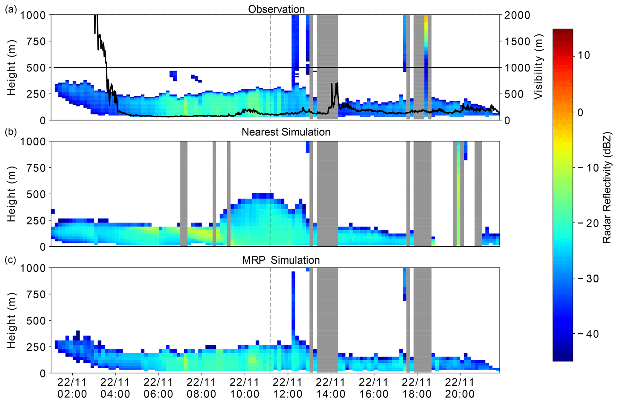
Figure 7Radar reflectivity and surface level visibility from a fog event at SIRTA observed on 22 November 2018 (a), simulated from the nearest grid point (b), and with the MRP selection method (c). The dashed black line indicates the time at which the following plot of reflectivity profiles is taken. These plots show the reflectivity for all profiles; profiles containing rain have been masked over in grey.
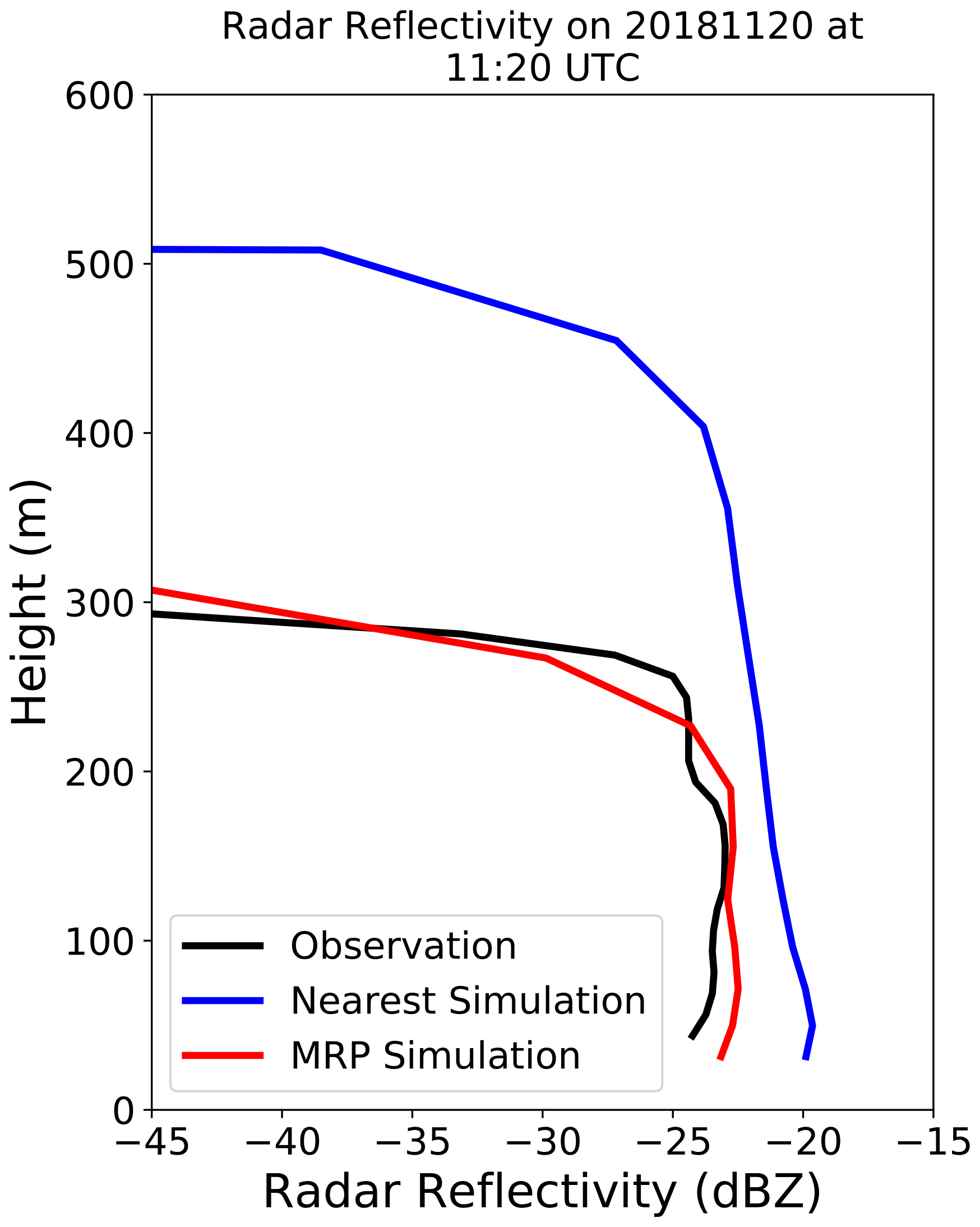
Figure 8Radar reflectivity profiles of the observation, simulation from the nearest grid point, and MRP simulation from the mature phase of the fog event at SIRTA on 22 November 2018. At this point in the fog event, the model overestimated the thickness of the fog layer by around 33 %.
4.3 Contoured frequency by altitude diagrams
In order to investigate the capability of the forward model to reproduce the overall structure of observed reflectivity, contoured frequency by altitude diagrams (CFADs; Yuter and Houze, 1995) calculated both from the observations and the simulations were compared in Fig. 9. In these figures, the number of cases in each radar reflectivity bin and each altitude level are shown between 50 to 1000 m with a bin width of 1 dB. The distributions at each height level were then normalized and the relative frequency of each bin is shown on the plots. The CFADs were plotted using data for which reflectivity at each range gate was obtained from the observation, from the nearest corresponding profile and from the MRP.
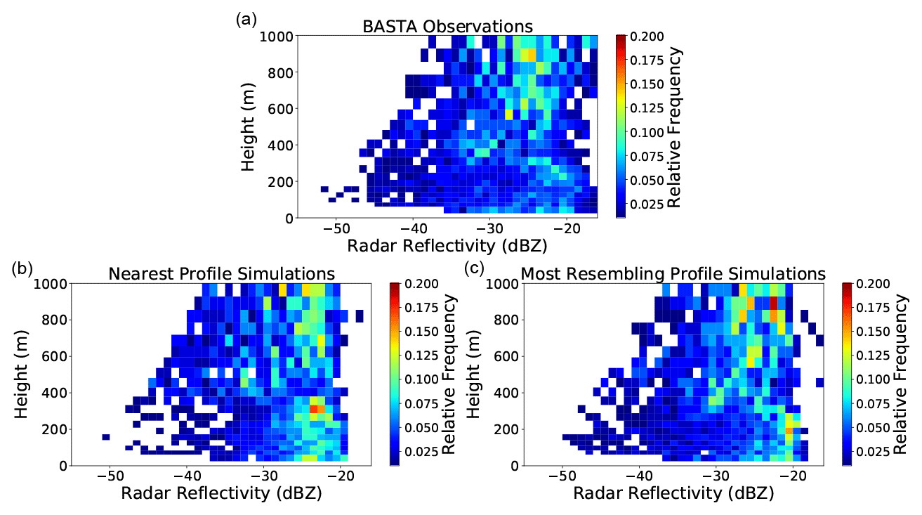
Figure 9CFADs of reflectivity observed and simulated from the nearest corresponding and most resembling profiles for the period 1 November 2018 to 19 February 2019 where cloud is seen in all three frames.
In the observations, the reflectivity in the lower 300 m is most concentrated between −30 to −20 dBZ and becomes gradually less concentrated at lower reflectivities. This contrasts the nearest corresponding profile simulations where there are significantly fewer radar reflectivities below −30 dBZ, and a concentration of higher values around −25 dBZ. This distribution is improved by the implementation of the MRP method, where a more even distribution of reflectivities is seen in the bottom 400 m. Though the distribution of simulated reflectivity generally improves using the MRP method, a large concentration of values between −23 and −20 dBZ persists, which is not seen in the observation CFAD.
4.4 Statistics on reflectivity innovations
For the period in which the fog classification was previously applied, between November 2018 and February 2019, radar reflectivity was simulated for the 28 km by 28 km domain for the entire period, after which the MRP method was applied. The observations were downscaled to the resolution of the simulations using the observation that corresponded most closely to the time of the simulation and using the bin corresponding most closely to the level heights of the model.
The radar simulator relies on the Mie approximation to derive the radar reflectivity. This approximation is valid for uniform spherical particles, which may be assumed for liquid cloud droplets. However, for snow, graupel, ice, and rain, whose shape can be significantly more complex, this approximation can no longer be assumed to be valid and larger errors of simulated reflectivity are likely to be caused. It was therefore decided to limit this study to reflectivity differences only due to the hydrometeors that are mainly responsible for fog in the mid-latitudes in winter: liquid water droplets. For the observation, a mask proxy was provided by the developers of the BASTA instrument to classify the hydrometeor type. The mask was used to reject from the statistical analysis cloud radar observations containing rain, drizzle, and ice below 200 m in the observations.
In the model space, a mask based on simulated reflectivity was used to discern whether rain, ice, snow, or graupel significantly contributed to the simulated reflectivity. This was made by finding reflectivity differences between the simulations containing all hydrometeors and the simulations for only cloud liquid water. Profiles containing significant reflectivity differences (of greater than 3 dB) were masked. This value was chosen as a 3 dB increase in radar reflectivity corresponds to a doubling of the received power. This effectively means that where differences between radar reflectivity simulated with only liquid water and radar reflectivity simulated with all hydrometeors exceeds 3 dB, the other hydrometeors contribute more to the radar reflectivity than liquid water content. Due to the effect of the attenuated signal that occurs when the radar signal passes through a rain event but impacts the readings above as well as inside the rainy atmosphere, where rain was found below 200 m, the entire profiles were also removed from the statistical calculations.
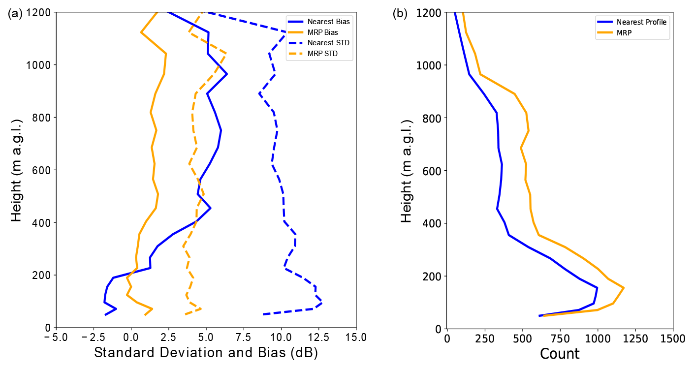
Figure 10(a) The bias and standard deviation of observation–simulated radar reflectivity at SIRTA for the period 1 November 2018–19 February 2019. The statistics were calculated for instances when reflectivity was both observed and simulated at a given range gate at a given time. (b) The count of cells for which reflectivity was observed and simulated.
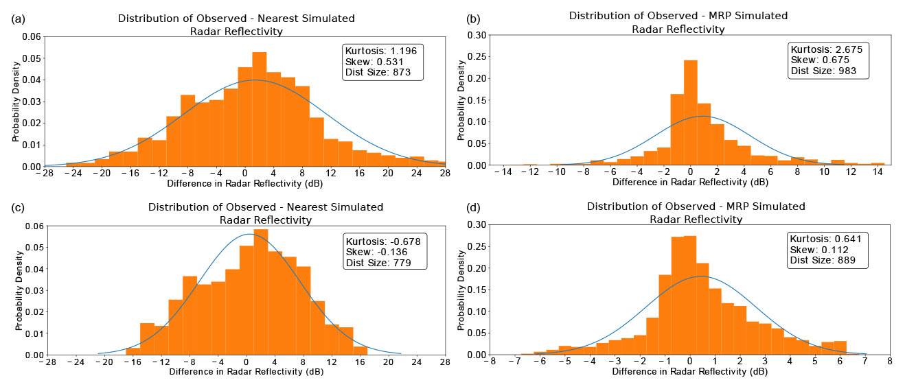
Figure 11(a)–(d) Distribution of observed minus simulated reflectivity errors for the nearest corresponding profile when no data are excluded, the MRP when no data are excluded, the nearest corresponding profile when 10 % of data are excluded, and the MRP when 10 % of data are excluded. All distributions are shown at 80 m a.g.l. for reflectivity innovations when there is signal both in the simulation and observation above the sensitivity threshold. The blue line shows the Gaussian distribution with the same mean and standard deviation.
Innovations (the difference between observed values and simulated values) were then calculated with the simulations for the nearest corresponding grid point and the MRP selection method. For these calculations, data were only used for which the range gate in both the simulation and observation had reflectivity signal above the sensitivity of the instrument. Figure 10 shows the standard deviation and bias at each height level. Statistics are shown up to 1200 m altitude, as above this height not enough cases without significant impact from ice can be selected. It is seen in the plots that both the bias and standard deviation are reduced at almost all heights with the implementation of the MRP method. The standard deviation was highest for the nearest profile at a height of 80 m a.g.l., for which the standard deviation was 12.6 dB. The MRP selection method was able to reduce this value to 4.7 dB, showing an improvement of 7.9 dB. Between 400 and 1000 m, the bias for the nearest profile was between 4.7 and 6.2 dB. For the MRP, it remained below 1.5 dB for the same height range. The improvement in the standard deviation is also seen in Fig. 11, in which the use of the MRP causes the distribution of reflectivity innovations to become narrower. It is also seen that using the MRP method increases the count and hence more retrievals may be made with this method compared to the nearest grid point method. This study shows that after removal of the largest background errors, the forward operator used in this study is able to replicate similar values of radar reflectivity from the background profiles, compared to the profiles observed during fog conditions. For the application of future 1D-Var retrievals and data assimilation, this brings the benefit of the simulations not needing to be bias-corrected. The reduction in the standard deviation may also improve the accuracy of the retrieved profiles.
Additionally, data assimilation relies on the assumption that the distribution of background and observation errors are Gaussian. Though in real-world scenarios a perfectly Gaussian distribution is rarely observed, certain manual and statistical checks may be made to ensure that a distribution is approximately Gaussian. According to Bulmer (1979), one of these checks is for the skewness and excess kurtosis of a distribution to be between −1 and 1. Figure 11 shows the distribution of innovations both for the co-located profile and the MRP profile at 80 m altitude. For the nearest profile, the Gaussianity is not satisfied, with values of skewness and excess kurtosis of 0.53 and 1.196 respectively. The MRP method did not satisfy this criteria either, with values of 0.68 and 2.68 respectively. This problem was due to the fact that more data were seen in the extremes of the distribution, with a reduction in the reflectivity differences for many cases but not being improved for some cases, for example when fog was not forecast at all throughout the domain. In order to rectify this, the most extreme 10 % of data points corresponding to the simulated errors above 16 dB for the nearest profile selection and 6.5 dB for the MRP were removed. After this data screening, the excess kurtosis for the nearest profile and MRP were reduced to 0.68 and 0.64 respectively demonstrating that distributions of innovations can be safely considered as Gaussian for future data assimilation steps. These conditions were also met for the distributions at higher levels (not shown).
In preparation of future data assimilation of newly developed 95 GHz cloud radar observations, this work aimed to better understand the uncertainties associated with background, observation, and forward operator errors during fog events.
An overview of fog forecast errors was firstly made using an instrumental dataset from SIRTA, Paris, during winter 2018–2019. It was concluded that the AROME model tends to over-forecast fog, with 1.6 times the amount of fog profiles being forecast compared to those observed over the investigation period. It was also shown that the model tends to over-forecast the fog top height, and that fog forecasts are prone to temporal errors of up to 3 h. Fog presence was also shown to display significant spatial variation in the model. For times in which the fog top height was well predicted by the model, however, the liquid water path was also well predicted, with a standard deviation in LWP difference of 26.4 g m−2 when the fog top height had a difference of less than 25 m and there was no cloud aloft.
In order to correct for modelling errors, a method for selecting the model profile that best resembles the observed profile was proposed. This contained a weighting function to ensure that the selected profile is optimized for fog, in case there were also clouds aloft in the observed profile.
As previously discussed, variational retrieval methods assume un-biased and normally distributed background and observation errors. In order to assess whether these conditions were met, statistics of the differences between observations and simulated reflectivity were calculated for both the nearest corresponding profile and the MRP. It was found that whilst there was a significant bias for the nearest corresponding profile (−2 to 5 dB below 1000 m) this was greatly reduced for the MRP (0 to 1.5 dB below 1000 m). The standard deviation was also reduced from 10.1 to 4.7 dB at 200 m through the implementation of the MRP method. When testing the distributions for normality, it was necessary to exclude 10 % of the data (limiting the innovations to −17 to 17 dB for the nearest profile selection method and −6.5 to 6.5 dB from the MRP method) in order for the excess kurtosis requirements to be met.
The contribution of uncertainties in the radar simulator due to assumptions on the droplet size distribution was also analysed. The uncertainty due to shape parameters of the cloud droplet size distribution was assessed to be 6.1 dB. Although this value seems large considering that the standard deviation of innovation errors was reduced to less than 5dB with the MRP method, the use of a two-moment microphysical scheme, such as LIMA (Vié et al., 2016), which is currently being tested for operational use, promises to reduce this error by a prognostic evolution of the droplet number concentration. Future methods of OE retrieval with cloud radar could also include the droplet number concentration and size distribution parameters in the set of variables to be retrieved. In this case, uncertainties from microphysical assumptions could be greatly reduced. Indeed, the significant sensitivity of the radar simulator towards droplet size distribution properties, as shown in this study, could prove to be advantageous for retrievals of these properties. The need for a background covariance matrix to include the additional variables, as well as a lack of additional observations that could constrain the retrieval means that this would, however, add additional complexity.
The results shown here indicate the suitability of the method for future 1D-Var retrievals of liquid water content profiles from the BASTA cloud radar by using an appropriate background profile from the AROME model and a consistent radar simulator. The benefits of this could be seen through the assimilation of the retrieved profiles into a high-resolution model as well as by deriving continuous measurements of the liquid water content profile throughout the boundary layer, which would be of particular use to fog process studies. When a better agreement was found between the background profile and observation, the radar simulator was also found to be suitable to simulate the BASTA cloud radar reflectivity during fog conditions, paving the way for larger model evaluations during fog events.
The AROME forecasts are available upon request from https://donneespubliques.meteofrance.fr/ (Météo France, 2021) or by request to pauline.martinet@meteo.fr. Data used from SIRTA are publicly available from http://sirta.ipsl.fr/ (Site Instrumental de Recherche par Télédétection Atmosphérique, 2021). The cloud radar data were an updated version of those publicly available from the SIRTA website, and requests for these can be made to julien.delanoe@latmos.ipsl.fr.
AB performed the analysis documented in the paper. PM, OC, and BV supervised this analysis. JD provided the cloud radar data and relevant assistance. JCD provided the data from SIRTA. MB provided the radar simulator.
The authors declare that they have no conflict of interest.
This article is part of the special issue “Tropospheric profiling (ISTP11) (AMT/ACP inter-journal SI)”. It is a result of the 11th edition of the International Symposium on Tropospheric Profiling (ISTP), Toulouse, France, 20–24 May 2019.
The authors thank Yann Seity for his help in setting up the AROME model. We extend our acknowledgements to the technical and computer staff of the SIRTA Observatory for making the observations and allowing the dataset to be easily accessible.
This work has been funded by the French ANR SOFOG3D (South west FOG 3D experiment for processes study, grant no. ANR-18-CE01-0004).
This paper was edited by V. Chandrasekar and reviewed by Alain Protat and two anonymous referees.
American Meteorological Society: Fog. Glossary of Meteorology, available at: http://glossary.ametsoc.org/wiki/fog, last access: 5 July 2021. a
Atlas, D.: The estimation of cloud parameters by radar, J. Meteorol., 11, 309–317, 1954. a
Bauer, P., Moreau, E., Chevallier, F., and O'keeffe, U.: Multiple-scattering microwave radiative transfer for data assimilation applications, Q. J. Roy. Meteor. Soc., 132, 1259–1281, 2006. a
Bohren, C. F. and Huffman, D. R.: Absorption and scattering of light by small particles, WILEY-VCH Verlag GmbH & Co. KGaA, Weinheim, 2008. a
Borderies, M., Caumont, O., Augros, C., Bresson, É., Delanoë, J., Ducrocq, V., Fourrié, N., Bastard, T. L., and Nuret, M.: Simulation of W-band radar reflectivity for model validation and data assimilation, Q. J. Roy. Meteor. Soc., 144, 391–403, 2018. a, b, c
Bouttier, F. and Courtier, P.: Data assimilation concepts and methods. Presented at the Meteorological Training Course Lecture Series, European Centre for Medium-Range Weather Forecasts, Reading, England, 1–58pp., 2002. a
Bulmer, M. G.: Principles of Statistics, Dover Publications, New York, NY, 1979. a
Crewell, S. and Löhnert, U.: Accuracy of cloud liquid water path from ground-based microwave radiometry 2. Sensor accuracy and synergy, Radio Sci., 38, 8042, https://doi.org/10.1029/2002RS002634, 2003. a
Cuxart, J., Bougeault, P., and Redelsperger, J.-L.: A turbulence scheme allowing for mesoscale and large-eddy simulations, Q. J. Roy. Meteor. Soc., 126, 1–30, 2000. a
De Angelis, F., Cimini, D., Löhnert, U., Caumont, O., Haefele, A., Pospichal, B., Martinet, P., Navas-Guzmán, F., Klein-Baltink, H., Dupont, J.-C., and Hocking, J.: Long-term observations minus background monitoring of ground-based brightness temperatures from a microwave radiometer network, Atmos. Meas. Tech., 10, 3947–3961, https://doi.org/10.5194/amt-10-3947-2017, 2017. a
Delanoë, J., Protat, A., Vinson, J.-P., Brett, W., Caudoux, C., Bertrand, F., Parent du Chatelet, J., Hallali, R., Barthes, L., Haeffelin, M., and Dupont, J. C.: BASTA: A 95-GHz FMCW Doppler radar for cloud and fog studies, J. Atmos. Ocean. Tech., 33, 1023–1038, 2016. a, b, c, d
Dombrowski-Etchevers, I., Seity, Y., Mestre, O., and Willemet, J.-M.: New algorithms for two forecasted products of weather: visibilities and 2 precipitation types, to be submitted, 2021. a
Ducongé, L., Lac, C., Vié, B., Bergot, T., and Price, J. D.: Fog in heterogeneous environments: the relative importance of local and non-local processes on radiative-advective fog formation, Q. J. Roy. Meteor. Soc., 146, 2522–2546, https://doi.org/10.1002/qj.3783, 2019. a
Dupont, J., Haeffelin, M., Stolaki, S., and Elias, T.: Analysis of dynamical and thermal processes driving fog and quasi-fog life cycles using the 2010–2013 ParisFog dataset, Pure Appl. Geophys., 173, 1337–1358, 2016. a
Dupont, J.-C., Haeffelin, M., Protat, A., Bouniol, D., Boyouk, N., and Morille, Y.: Stratus–fog formation and dissipation: a 6-day case study, Bound.-Lay. Meteorol., 143, 207–225, 2012. a
Ebell, K., Löhnert, U., Päschke, E., Orlandi, E., Schween, J. H., and Crewell, S.: A 1-D variational retrieval of temperature, humidity, and liquid cloud properties: Performance under idealized and real conditions, J. Geophys. Res.-Atmos., 122, 1746–1766, https://doi.org/10.1002/2016JD025945, 2017. a
Fielding, M. and Janiskova, M.: Direct 4D-Var assimilation of space-borne cloud radar reflectivity and lidar backscatter. Part I: Observation operator and implementation, Q. J. Roy. Meteor. Soc., 146, 3877–3899, https://doi.org/10.1002/qj.3878, 2020. a
Fouquart, Y. and Bonnel, B.: Computations of solar heating of the Earth's atmosphere: A new parameterization, Beiträge zur Physik der Atmosphäre, 53, 35–62, 1980. a
Geoffroy, O., Brenguier, J.-L., and Burnet, F.: Parametric representation of the cloud droplet spectra for LES warm bulk microphysical schemes, Atmos. Chem. Phys., 10, 4835–4848, https://doi.org/10.5194/acp-10-4835-2010, 2010. a, b
Gultepe, I., Tardif, R., Michaelides, S. C., Cermak, J., Bott, A., Bendix, J., Müller, M. D., Pagowski, M., Hansen, B., Ellrod, G., and Jacobs, W.: Fog research: A review of past achievements and future perspectives, Pure Appl. Geophys., 164, 1121–1159, 2007. a
Haeffelin, M., Barthès, L., Bock, O., Boitel, C., Bony, S., Bouniol, D., Chepfer, H., Chiriaco, M., Cuesta, J., Delanoë, J., Drobinski, P., Dufresne, J.-L., Flamant, C., Grall, M., Hodzic, A., Hourdin, F., Lapouge, F., Lemaître, Y., Mathieu, A., Morille, Y., Naud, C., Noël, V., O'Hirok, W., Pelon, J., Pietras, C., Protat, A., Romand, B., Scialom, G., and Vautard, R.: SIRTA, a ground-based atmospheric observatory for cloud and aerosol research, Ann. Geophys., 23, 253–275, https://doi.org/10.5194/angeo-23-253-2005, 2005. a, b
Haeffelin, M., Laffineur, Q., Bravo-Aranda, J.-A., Drouin, M.-A., Casquero-Vera, J.-A., Dupont, J.-C., and De Backer, H.: Radiation fog formation alerts using attenuated backscatter power from automatic lidars and ceilometers, Atmos. Meas. Tech., 9, 5347–5365, https://doi.org/10.5194/amt-9-5347-2016, 2016. a
Hu, J., Yussouf, N., Turner, D. D., Jones, T. A., and Wang, X.: Impact of ground-based remote sensing boundary layer observations on short-term probabilistic forecasts of a tornadic supercell event, Weather Forecast., 34, 1453–1476, 2019. a
Janisková, M.: Assimilation of cloud information from space-borne radar and lidar: experimental study using a 1D+ 4D-Var technique, Q. J. Roy. Meteorol. Soc., 141, 2708–2725, 2015. a
Kollias, P., Clothiaux, E. E., Miller, M., Albrecht, B. A., Stephens, G., and Ackerman, T.: Millimeter-wavelength radars: New frontier in atmospheric cloud and precipitation research, B. Am. Meteorol. Soc., 88, 1608–1624, 2007. a
Lac, C., Chaboureau, J.-P., Masson, V., Pinty, J.-P., Tulet, P., Escobar, J., Leriche, M., Barthe, C., Aouizerats, B., Augros, C., Aumond, P., Auguste, F., Bechtold, P., Berthet, S., Bielli, S., Bosseur, F., Caumont, O., Cohard, J.-M., Colin, J., Couvreux, F., Cuxart, J., Delautier, G., Dauhut, T., Ducrocq, V., Filippi, J.-B., Gazen, D., Geoffroy, O., Gheusi, F., Honnert, R., Lafore, J.-P., Lebeaupin Brossier, C., Libois, Q., Lunet, T., Mari, C., Maric, T., Mascart, P., Mogé, M., Molinié, G., Nuissier, O., Pantillon, F., Peyrillé, P., Pergaud, J., Perraud, E., Pianezze, J., Redelsperger, J.-L., Ricard, D., Richard, E., Riette, S., Rodier, Q., Schoetter, R., Seyfried, L., Stein, J., Suhre, K., Taufour, M., Thouron, O., Turner, S., Verrelle, A., Vié, B., Visentin, F., Vionnet, V., and Wautelet, P.: Overview of the Meso-NH model version 5.4 and its applications, Geosci. Model Dev., 11, 1929–1969, https://doi.org/10.5194/gmd-11-1929-2018, 2018. a
Lafore, J. P., Stein, J., Asencio, N., Bougeault, P., Ducrocq, V., Duron, J., Fischer, C., Héreil, P., Mascart, P., Masson, V., Pinty, J. P., Redelsperger, J. L., Richard, E., and Vilà-Guerau de Arellano, J.: The Meso-NH Atmospheric Simulation System. Part I: adiabatic formulation and control simulations, Ann. Geophys., 16, 90–109, https://doi.org/10.1007/s00585-997-0090-6, 1998. a
Le Bastard, T., Caumont, O., Gaussiat, N., and Karbou, F.: Combined use of volume radar observations and high-resolution numerical weather predictions to estimate precipitation at the ground: methodology and proof of concept, Atmos. Meas. Tech., 12, 5669–5684, https://doi.org/10.5194/amt-12-5669-2019, 2019. a
Li, Y.: Detection, Imaging and Characterisation of FogFields by Radar, PhD thesis, Delft University of Technology, Delft, the Netherlands, 2015. a
Liebe, H. J.: An updated model for millimeter wave propagation in moist air, Radio Sci., 20, 1069–1089, 1985. a
Liu, L., Ruan, Z., Zheng, J., and Gao, W.: Comparing and merging observation data from Ka-band cloud radar, C-band frequency-modulated continuous wave radar and ceilometer systems, Remote Sensing, 9, 1282, https://doi.org/10.3390/rs9121282, 2017. a
Liu, Y. and Daum, P. H.: Spectral dispersion of cloud droplet size distributions and the parameterization of cloud droplet effective radius, Geophys. Res. Lett., 27, 1903–1906, 2000. a
Maahn, M., Turner, D. D., Löhnert, U., Posselt, D. J., Ebell, K., Mace, G. G., and Comstock, J. M.: Optimal Estimation Retrievals and Their Uncertainties: What Every Atmospheric Scientist Should Know, B. Am. Meteorol. Soc., 101, E1512–E1523, https://doi.org/10.1175/BAMS-D-19-0027.1, 2020. a
Maier, F., Bendix, J., and Thies, B.: Simulating Z–LWC relations in natural fogs with radiative transfer calculations for future application to a cloud radar profiler, Pure Appl. Geophys., 169, 793–807, 2012. a
Martinet, P., Dabas, A., Donier, J.-M., Douffet, T., Garrouste, O., and Guillot, R.: 1D-Var temperature retrievals from microwave radiometer and convective scale model, Tellus A, 67, 27925, https://doi.org/10.3402/tellusa.v67.27925, 2015. a, b
Martinet, P., Cimini, D., De Angelis, F., Canut, G., Unger, V., Guillot, R., Tzanos, D., and Paci, A.: Combining ground-based microwave radiometer and the AROME convective scale model through 1DVAR retrievals in complex terrain: an Alpine valley case study, Atmos. Meas. Tech., 10, 3385–3402, https://doi.org/10.5194/amt-10-3385-2017, 2017. a
Martinet, P., Cimini, D., Burnet, F., Ménétrier, B., Michel, Y., and Unger, V.: Improvement of numerical weather prediction model analysis during fog conditions through the assimilation of ground-based microwave radiometer observations: a 1D-Var study, Atmos. Meas. Tech., 13, 6593–6611, https://doi.org/10.5194/amt-13-6593-2020, 2020. a
Martucci, G., Milroy, C., and O'Dowd, C. D.: Detection of cloud-base height using Jenoptik CHM15K and Vaisala CL31 ceilometers, J. Atmo. Ocean. Tech., 27, 305–318, 2010. a
Masson, V.: A physically-based scheme for the urban energy budget in atmospheric models, Bound.-Lay. Meteorol., 94, 357–397, 2000. a
Masson, V., Le Moigne, P., Martin, E., Faroux, S., Alias, A., Alkama, R., Belamari, S., Barbu, A., Boone, A., Bouyssel, F., Brousseau, P., Brun, E., Calvet, J.-C., Carrer, D., Decharme, B., Delire, C., Donier, S., Essaouini, K., Gibelin, A.-L., Giordani, H., Habets, F., Jidane, M., Kerdraon, G., Kourzeneva, E., Lafaysse, M., Lafont, S., Lebeaupin Brossier, C., Lemonsu, A., Mahfouf, J.-F., Marguinaud, P., Mokhtari, M., Morin, S., Pigeon, G., Salgado, R., Seity, Y., Taillefer, F., Tanguy, G., Tulet, P., Vincendon, B., Vionnet, V., and Voldoire, A.: The SURFEXv7.2 land and ocean surface platform for coupled or offline simulation of earth surface variables and fluxes, Geosci. Model Dev., 6, 929–960, https://doi.org/10.5194/gmd-6-929-2013, 2013. a
Mazoyer, M.: Impact du Processus d'Activation sur les Proprietes Microphysiques des Brouillards et Sur Leur Cycle de Vie, PhD thesis, Institut National Polytechnique de Toulouse, Toulouse, France, 2016. a, b, c
Mazoyer, M., Burnet, F., Denjean, C., Roberts, G. C., Haeffelin, M., Dupont, J.-C., and Elias, T.: Experimental study of the aerosol impact on fog microphysics, Atmos. Chem. Phys., 19, 4323–4344, https://doi.org/10.5194/acp-19-4323-2019, 2019. a
Météo France: Homepage, available at: https://donneespubliques.meteofrance.fr/, last access: 2021. a
Miles, N. L., Verlinde, J., and Clothiaux, E. E.: Cloud droplet size distributions in low-level stratiform clouds, J. Atmos. Sci., 57, 295–311, 2000. a
Mlawer, E. J., Taubman, S. J., Brown, P. D., Iacono, M. J., and Clough, S. A.: Radiative transfer for inhomogeneous atmospheres: RRTM, a validated correlated-k model for the longwave, J. Geophys. Res.-Atmos., 102, 16663–16682, 1997. a
Müller, M., Masbou, M., and Bott, A.: Three‐dimensional fog forecasting in complex terrain, Q. J. Roy. Meteorol. Soc., 136, 2189–2202, https://doi.org/10.1002/qj.705, 2010. a
NRC: Observing weather and climate from the ground up: A nationwide network of networks, National Academies Press, Washington D. C., 2009. a
Philip, A., Bergot, T., Bouteloup, Y., and Bouyssel, F.: The impact of vertical resolution on fog forecasting in the kilometric-scale model arome: a case study and statistics, Weather Forecast., 31, 1655–1671, 2016. a, b, c, d
Pinty, J.-P. and Jabouille, P.: A mixed-phase cloud parameterization for use in mesoscale non-hydrostatic model: simulations of a squall line and of orographic precipitations, in: Conf. on Cloud Physics, Amer. Meteor. Soc Everett, WA, 17–21 August 1998, 217–220, 1998. a, b
Podzimek, J.: Droplet concentration and size distribution in haze and fog, Stud. Geophys. Geod., 41, 277–296, 1997. a
Rodgers, C. D.: Inverse Methods for Atmospheric Sounding Inverse Methods for Atmospheric Sounding, Theory and Practice, World Scientific, Singapore, 17–24 pp., 2000. a, b
Román-Cascón, C., Yagüe, C., Steeneveld, G.-J., Morales, G., Arrillaga, J. A., Sastre, M., and Maqueda, G.: Radiation and cloud-base lowering fog events: Observational analysis and evaluation of WRF and HARMONIE, Atmos. Res., 229, 190–207, 2019. a
Rose, T., Crewell, S., Löhnert, U., and Simmer, C.: A network suitable microwave radiometer for operational monitoring of the cloudy atmosphere, Atmos. Res., 75, 183–200, 2005. a
Schaefer, J. T.: The critical success index as an indicator of warning skill, Weather Forecast., 5, 570–575, 1990. a
Seifert, A. and Beheng, K. D.: A double-moment parameterization for simulating autoconversion, accretion and selfcollection, Atmos. Res., 59, 265–281, 2001. a
Seity, Y., Brousseau, P., Malardel, S., Hello, G., Bénard, P., Bouttier, F., Lac, C., and Masson, V.: The AROME-France convective-scale operational model, Mon. Weather Rev., 139, 976–991, 2011. a, b
Site Instrumental de Recherche par Télédétection Atmosphérique: Homepage, available at: http://sirta.ipsl.fr/, last access: 2021. a
Steeneveld, G., Ronda, R., and Holtslag, A.: The challenge of forecasting the onset and development of radiation fog using mesoscale atmospheric models, Bound.-Lay. Meteorol., 154, 265–289, 2015. a
Tardif, R. and Rasmussen, R. M.: Event-based climatology and typology of fog in the New York City region, J. Appl. Meteorol. Clim., 46, 1141–1168, 2007. a
Thies, B., Müller, K., Maier, F., and Bendix, J.: Fog monitoring using a new 94 GHz FMCW cloud radar, in: 5th International Conference on Fog, Fog Collection and Dew, Münster, Germany, 25–30 July 2010, available at: https://meetingorganizer.copernicus.org/FOGDEW2010/FOGDEW2010-103.pdf (last access: 8 June 2021), FOGDEW2010-103, 2010. a
Toledo, F., Delanoë, J., Haeffelin, M., Dupont, J.-C., Jorquera, S., and Le Gac, C.: Absolute calibration method for frequency-modulated continuous wave (FMCW) cloud radars based on corner reflectors, Atmos. Meas. Tech., 13, 6853–6875, https://doi.org/10.5194/amt-13-6853-2020, 2020. a
Vié, B., Pinty, J.-P., Berthet, S., and Leriche, M.: LIMA (v1.0): A quasi two-moment microphysical scheme driven by a multimodal population of cloud condensation and ice freezing nuclei, Geosci. Model Dev., 9, 567–586, https://doi.org/10.5194/gmd-9-567-2016, 2016. a
Wærsted, E.: Description of physical processes driving the life cycle of radiation fog and fog – stratus transitions based on conceptual models, PhD thesis, Paris Saclay, Paris, 2018. a
Wærsted, E. G., Haeffelin, M., Dupont, J.-C., Delanoë, J., and Dubuisson, P.: Radiation in fog: quantification of the impact on fog liquid water based on ground-based remote sensing, Atmos. Chem. Phys., 17, 10811–10835, https://doi.org/10.5194/acp-17-10811-2017, 2017. a
Wilczak, J., Finley, C., Freedman, J., Cline, J., Bianco, L., Olson, J., Djalalova, I., Sheridan, L., Ahlstrom, M., Manobianco, J., and Zack, J.: The Wind Forecast Improvement Project (WFIP): A public–private partnership addressing wind energy forecast needs, B. Am. Meteorol. Soc., 96, 1699–1718, 2015. a
Wriedt, T.: Mie theory: a review, in: The Mie Theory, Springer, Berlin, Heidelberg, https://doi.org/10.1007/978-3-642-28738-1_2, pp. 53–71, 2012. a
Yuter, S. E. and Houze, Jr., R. A.: Three-dimensional kinematic and microphysical evolution of Florida cumulonimbus. Part II: Frequency distributions of vertical velocity, reflectivity, and differential reflectivity, Mon. Weather Rev., 123, 1941–1963, 1995. a
Zhao, C., Zhao, L., and Dong, X.: A case study of stratus cloud properties using in situ aircraft observations over Huanghua, China, Atmosphere, 10, 19, https://doi.org/10.3390/atmos10010019, 2019. a