The high-frequency response correction of eddy covariance fluxes – Part 2: An experimental approach for analysing noisy measurements of small fluxes

Fluxes measured with the eddy covariance (EC) technique are subject to flux losses at high frequencies (low-pass filtering). If not properly corrected for, these result in systematically biased ecosystem–atmosphere gas exchange estimates. This loss is corrected using the system's transfer function which can be estimated with either theoretical or experimental approaches. In the experimental approach, commonly used for closed-path EC systems, the low-pass filter transfer function (H) can be derived from the comparison of either (i) the measured power spectra of sonic temperature and the target gas mixing ratio or (ii) the cospectra of both entities with vertical wind speed. In this study, we compare the power spectral approach (PSA) and cospectral approach (CSA) in the calculation of H for a range of attenuation levels and signal-to-noise ratios (SNRs). For a systematic analysis, we artificially generate a representative dataset from sonic temperature (T) by attenuating it with a first order filter and contaminating it with white noise, resulting in various combinations of time constants and SNRs. For PSA, we use two methods to account for the noise in the spectra: the first is the one introduced by Ibrom et al. (2007a) (PSA_I07), in which the noise and H are fitted in different frequency ranges, and the noise is removed before estimating H. The second is a novel approach that uses the full power spectrum to fit both H and noise simultaneously (PSA_A21). For CSA, we use a method utilizing the square root of the H with shifted vertical wind velocity time series via cross-covariance maximization (${\text{CSA}}_{\sqrt{H},\mathrm{sync}}$). PSA_I07 tends to overestimate the time constant when low-pass filtering is low, whilst the new PSA_A21 and ${\text{CSA}}_{\sqrt{H},\mathrm{sync}}$ successfully estimate the expected time constant regardless of the degree of attenuation and SNR. We further examine the effect of the time constant obtained with the different implementations of PSA and CSA on cumulative fluxes using estimated time constants in frequency response correction. For our example time series, the fluxes corrected using time constants derived by PSA_I07 show a bias between 0.1 % and 1.4 %. PSA_A21 showed almost no bias, while ${\text{CSA}}_{\sqrt{H},\mathrm{sync}}$ showed bias of ±0.4 %. The accuracies of both PSA and CSA methods were not significantly affected by SNR level, instilling confidence in EC flux measurements and data processing in set-ups with low SNR. Overall we show that, when using power spectra for the empirical estimation of parameters of H for closed-path EC systems the new PSA_A21 outperforms PSA_I07, while when using cospectra the ${\text{CSA}}_{\sqrt{H},\mathrm{sync}}$ approach provides accurate results. These findings are independent of the SNR value and attenuation level.

1 Introduction

Vertical turbulent fluxes of momentum, energy, and gases between the atmosphere and the biosphere measured by the eddy covariance (EC) technique are subject to both low- and high-frequency losses (Foken, 2008; Aubinet et al., 2012). The physical limitations in instrument response times, spatial separation of instruments, line averaging, and air transport through the sampling tubes cause high-frequency losses (Aubinet et al., 1999).

The EC sampling system acts as a low-pass filter on the flux, and the signal loss must be compensated for with the frequency response correction (FRC) during post-processing. The first step in the FRC is the description of the effect of the low-pass filtering of the measurement system, and for this, the transfer function approach has been widely used since it was first proposed by Moore (1986). The joint transfer function (H) that describes the low-pass filtering of the whole EC system can be determined theoretically or experimentally (Foken, 2008; Aubinet et al., 2012). The theoretical approach involves various specific transfer functions that are estimated to represent different causes of flux loss. Conversely, in the experimental approach H is estimated from in situ measurements. Due to its simplicity, many studies have implemented the theoretical approach, which typically works well with fluxes measured by open-path EC systems, as well as momentum fluxes and sensible heat fluxes measured by sonic anemometers (Aubinet et al., 2012). However, for complex EC systems the necessary information to calculate H is not available and needs to be estimated empirically. In addition, the time response of the system can vary with relative humidity (Ibrom et al., 2007a), tube ageing (Mammarella et al., 2009), and variations in the flow regime in the tube. Thus, the theoretical approach is not preferred for gas fluxes measured with closed-path EC systems, for which the experimental approach is therefore recommended (Aubinet et al., 2012; Sabbatini et al., 2018; Nemitz et al., 2018).

In the experimental approach for closed-path systems, H is usually estimated from either the measured power spectra (i.e. PSA) or cospectra (i.e. CSA) of sonic temperature and the mixing ratio of the target gas (χ). Different studies use either PSA (Ibrom et al., 2007a; Nordbo et al., 2011; Fratini et al., 2012; Sabbatini et al., 2018) or CSA (Aubinet et al., 1999; Humphreys et al., 2005; Mammarella et al., 2009; Peltola et al., 2013). Also, some software packages used for EC flux calculation are based on PSA (e.g. EddyPro, see LI-COR Biosciences, 2020), while others are based on CSA (e.g. EddyUH, see Mammarella et al., 2016).

Interestingly, there has not been much debate to date whether to use power spectra or cospectra to determine the time constant of the H (or response time), which characterizes the EC system's high-frequency response. Only recently, Wintjen et al. (2020) investigated the optimal method for high-frequency response correction, for fluxes of nitrogen compounds, recommending CSA. Ibrom et al. (2007a) argued for using PSA as the vertical wind speed (w) does not contain any relevant information for the spectral attenuation of the gas collection and data acquisition system, allowing us to describe sensor-related attenuation independently. This should in principle provide a better estimation of the time constant of the gas analysis system because the spectral data are not mingled with other components, such as, for example, sensor separation. In this approach, the effect of sensor separation is then treated explicitly with an additional correction step (Horst and Lenschow, 2009). In most cases the instrumental noise becomes visible in the high-frequency range of χ^′ power spectra, and this has to be dealt with before the time constant of the gas sampling system can be estimated. The noise removal procedure is not well established, and this represents a major uncertainty in the PSA approach. This paper explores this uncertainty and proposes a novel, more robust approach to account for the noise in PSA.

On the other hand, this noise is often assumed not to correlate with the fluctuations in w, and therefore it does not contribute to the cospectra between w and χ. If this holds, this makes the CSA attractive for the estimation of the time constant because then the noise would effectively disappear from the measured signal. Yet, the use of the CSA relies on the correct determination of the time lag between w and χ, which may be difficult in the case of small fluxes due to noisier cross-correlation function, making the search for the absolute maximum harder (Langford et al., 2015). Due to the above-mentioned reasons, empirically determined H can be a source of uncertainty for the FRC (Lee et al., 2004). Additionally, the CSA approach inadvertently accounts for the phase shift caused by low-pass filtering, a topic discussed in our companion paper (Peltola et al., 2021).

EC measurements conducted under low-flux conditions result in relatively high signal noise, i.e. low signal-to-noise ratio (SNR) (Smeets et al., 2009). EC fluxes with low SNR are normally found in many ecosystems especially for methane (CH₄) and nitrous oxide (N₂O), as well as for other non-H₂O and non-CO₂ gas species and aerosol particles, in which any implementation of the FRC becomes uncertain (Rannik et al., 2015; Nemitz et al., 2018; Oosterwijk et al., 2018). Low SNR can also be observed for CO₂ in specific ecosystems (e.g. lakes) and seasons (e.g. senescence, winter dormancy) for CH₄ over well-drained soils or peatlands during winter and for N₂O in long periods outside the high emission periods (e.g. fertilizer applications, freeze–thaw cycles, or rain events), all of which, although small, significantly contribute to the long-term flux budgets and, hence, must be corrected to reduce the systematic bias. Thus, the investigation of uncertainties in commonly used FRC methods is of great importance for obtaining unbiased, harmonized, and continuous time series of gas fluxes measured by EC technique.

To our knowledge, the uncertainty in fluxes caused by the use of the PSA and the CSA has not been investigated systematically so far, motivating this study, which hypothesizes that the success of the PSA and CSA usage in FRC depends on the attenuation condition and the level of SNR. Consequently, we expect to see substantially different time constants, correction factors, and eventually different overall magnitudes of correction estimates with respect to the attenuation and SNR conditions. To test this hypothesis, we need a scalar dataset which represents different attenuation levels and noise conditions. Assuming spectral similarity between scalars, we apply different levels of attenuation and noise to sonic temperature time series (T) in order to generate a proxy representing an attenuated gas concentration dataset (e.g. CH₄, N₂O) with known characteristics. We use a first-order low-pass filter which solely depends on a single time constant (τ_LPF) to attenuate the signal. Then, we systematically contaminate the signal with white noise. We then assess which analysis approach most closely retrieves the true time constant used to degrade the flux in the first place. First, we try to retrieve the system time constants using the PSA and CSA and then compare those with original values (i.e. τ_LPF). Second, in order to demonstrate how variation in time constant estimation further affects the cumulative fluxes, we run a low-pass filter over 1-month-long time series of T and correct the attenuation with the FRC of Fratini et al. (2012) via implementing the time constants calculated in the first step. In Sect. 2, the theory of experimental FRC is summarized. In Sect. 3, materials used in this study and methods are explained. Results and discussion are then interpreted in Sect. 4.

2 Theory

2.1 Background of methods typically used to determine the system time response

In order to calculate the true unattenuated (i.e. frequency-response corrected) covariance (${\stackrel{\mathrm{‾}}{w^{\prime }{\mathit{\chi }}^{\prime }}}_{\mathrm{corr}}$) with the transfer function method, the measured covariance (${\stackrel{\mathrm{‾}}{w^{\prime }{\mathit{\chi }}^{\prime }}}_{\mathrm{meas}}$) is multiplied by a correction factor (F_corr):

$$\begin{array}{}\text{(1)}& {\stackrel{\mathrm{‾}}{w^{\prime }{\mathit{\chi }}^{\prime }}}_{\mathrm{corr}}={\stackrel{\mathrm{‾}}{w^{\prime }{\mathit{\chi }}^{\prime }}}_{\mathrm{meas}}{F}_{\mathrm{corr}}.\end{array}$$

One way to calculate F_corr is to estimate the ratio of the integrated unbiased and biased cospectra as a function of frequency. In order to define the cospectrum of the unattenuated scalar under the assumption that the normalized cospectrum of all scalars has the same form (i.e scalar similarity), either the cospectra model (see Mammarella et al., 2009) or the measured cospectra (see Fratini et al., 2012) of T are used as a reference. Many studies used the surface layer models described by Kaimal et al. (1972) and based on Kansas experiments (see Moore, 1986). The attenuated cospectra are obtained by multiplication of the reference cospectra with the transfer function (H), which characterizes the filtering of the EC system.

Another way to calculate F_corr is to simulate the attenuation with a recursive filter in time rather than in frequency space, in which F_corr is defined as the ratio of the unattenuated and attenuated covariances (see Goulden et al., 1997). In addition, based on the same approach, an experimental method was proposed by Ibrom et al. (2007a) to parameterize the correction factor separately for stable and unstable stratifications using meteorological data. For this method, a further modification was later suggested by Fratini et al. (2012) for the processing of large fluxes.

Regardless of the method chosen, H needs to be obtained either theoretically or empirically before F_corr can be calculated. In the empirical approach, H can be determined using in situ measurements as a ratio of the normalized power spectra (for PSA) or cospectra (for CSA) of the attenuated scalar to those of an unattenuated scalar, e.g. T. In both approaches, in order to reduce the uncertainties in the low-frequency part of the spectra and to fulfil the assumption of spectral similarity, data must be selected from periods with rigorous stationary turbulent mixing. In addition, the power spectra and cospectra of T and χ should be normalized with their standard deviations so that they can be compared with each other (see their Eq. 2 in Ibrom et al., 2007a).

For the PSA, H can be calculated using the power spectra of χ and T (Eq. 2), in which the effect of sensor separation should additionally be treated via the method proposed by Horst and Lenschow (2009). For PSA, H is derived as

$$\begin{array}{}\text{(2)}& H_{\mathrm{PSA}}\left(f\right)=\left[{\displaystyle \frac{S_{\mathit{\chi }}\left(f\right)}{{\mathit{\sigma }}_{\mathit{\chi }}^{\mathrm{2}}}}\right][{\displaystyle \frac{S_T\left(f\right)}{{\mathit{\sigma }}_T^{\mathrm{2}}}}{]}^{-\mathrm{1}},\end{array}$$

where S_χ indicates the power spectrum of measured target gas mixing ratio, S_T is the power spectrum of T, and variances (${\mathit{\sigma }}_{\mathit{\chi }}^{\mathrm{2}}$ and ${\mathit{\sigma }}_T^{\mathrm{2}}$) are calculated across the frequency range over which no attenuation occurs. Instrumental noise often becomes dominant in the high-frequency range of the power spectrum and also contributes to σ_χ (see blue line in Fig. 1).

Thus, prior to the calculation of Eq. (2), the noise contribution to the power spectra of S_χ should be removed (Ibrom et al., 2007a). Finally, the frequency dependence of H_PSA can be described through a sigmoidal curve which is characterized by the time constant (τ) of the measurement system (for more details see Peltola et al., 2021, and references therein):

$$\begin{array}{}\text{(3)}& H_{\mathrm{emp}}\left(f\right)={\displaystyle \frac{\mathrm{1}}{\mathrm{1}+(\mathrm{2}\mathit{\pi }f\mathit{\tau }{)}^{\mathrm{2}}}}.\end{array}$$

For PSA, Ibrom et al. (2007a) updated Eq. (2) by introducing a normalization factor which is used to secure the spectral similarity especially for small fluxes. As described in their Eq. (6), the time constant and the normalization factor (F_n) are obtained by fitting the following equation to the dampened and noise-free χ data:

$$\begin{array}{}\text{(4)}& {\displaystyle \frac{S_{\mathit{\chi }}\left(f\right)}{{\mathit{\sigma }}_{\mathit{\chi }}^{\mathrm{2}}}}={\displaystyle \frac{S_T\left(f\right)}{{\mathit{\sigma }}_T^{\mathrm{2}}}}{F}_{\mathrm{n}}{\displaystyle \frac{\mathrm{1}}{\mathrm{1}+(\mathrm{2}\mathit{\pi }f\mathit{\tau }{)}^{\mathrm{2}}}}.\end{array}$$

In our study, we follow the same procedure (hereafter PSA_I07) for the time constant calculation for the PSA, which is summarized in Sect. 3.2. In addition to PSA_I07, we used a new comprehensive method for PSA, which is summarized in Sect. 2.2.

Alternatively, for the CSA, H is calculated as

$$\begin{array}{}\text{(5)}& H_{\mathrm{CSA}}\left(f\right)=\left[{\displaystyle \frac{{\text{Co}}_{w\mathit{\chi }}\left(f\right)}{\stackrel{\mathrm{‾}}{w^{\prime }{\mathit{\chi }}^{\prime }}}}\right][{\displaystyle \frac{{\text{Co}}_{wT}\left(f\right)}{\stackrel{\mathrm{‾}}{w^{\prime }{T}^{\prime }}}}{]}^{-\mathrm{1}},\end{array}$$

where f is the natural frequency, Co_wχ indicates the cospectrum of measured w and target gas mixing ratio χ, Co_wT is the cospectrum of measured kinematic heat flux, and $\stackrel{\mathrm{‾}}{w^{\prime }{\mathit{\chi }}^{\prime }}$ and $\stackrel{\mathrm{‾}}{w^{\prime }{T}^{\prime }}$ are covariances calculated across a frequency range where the cospectra are not attenuated.

For CSA, τ is obtained via fitting H_emp to Eq. (5); however, there is an ongoing debate on whether the correct transfer function for the cospectra would be $\sqrt{H_{\mathrm{emp}}}$ instead of H_emp (Moore, 1986; Eugster and Senn, 1995; Horst, 1997, 2000; Fratini et al., 2012; Hunt et al., 2016), which is related to the low-pass filtering time lag (i.e. phase shift) as discussed thoroughly by Peltola et al. (2021). They showed that the phase shift effect can be approximated well when square root is used. We therefore opt to apply $\sqrt{H_{\mathrm{emp}}}$ to CSA.

2.2 Estimating the time constant from a noise-contaminated power spectrum

In the PSA_I07 application to noisy data, the time constant is typically obtained via two separate fitting procedure steps following the approach of Ibrom et al. (2007a) as illustrated in Fig. 1 for a noisy spectrum. First, in order to remove the noise, the noise part of the attenuated noisy power spectra (solid blue line) is fitted with a line of an unconstrained slope (dashed blue line) within the marked-frequency domain in the high-frequency end, and then the line is extended towards lower frequencies and subtracted from attenuated noisy power spectra, yielding noise-free power spectra (black line) represented with the term $\frac{S_{\mathit{\chi }}\left(f\right)}{{\mathit{\sigma }}_{\mathit{\chi }}^{\mathrm{2}}}$ in Eq. (4). The unattenuated and noise-free spectra of T (i.e. term $\frac{S_T\left(f\right)}{{\mathit{\sigma }}_T^{\mathrm{2}}}$ in Eq. 4) is represented with the red line. Second, the time constant is obtained via fitting Eq. (4) within the marked-frequency domain.

Regarding the noise removal procedure, this approach can be problematic as we will show in Sect. 4.1 below because if the resulting line (dashed blue line in Fig. 1) has a slope less than unity, its extrapolation to lower frequencies erroneously removes the true signal. In addition, the frequency domains used for fittings should be determined visually, requiring expertise in micrometeorology and signal processing, which limits its effective application in the research community.

Here we introduce a new alternative approach (hereafter PSA_A21) that overcomes above-mentioned shortcomings as we will show in Sect. 4.1 below. It performs the estimation of the time constant and accounts for instrumental noise without removal in a single non-linear comprehensive fitting step. In this approach, the time constant is yielded via fitting Eq. (7) to directly attenuated noisy power spectra (solid blue line). The fitting is performed across the entire frequency domain (Fig. 1), indicating that the visual inspection is not needed. The brief derivation of Eq. (7) is shown below.

Equation (4) can be extended to the following equation, which includes also the noise component of the scalar:

$$\begin{array}{}\text{(6)}& f{\displaystyle \frac{S_{\mathit{\chi }}\left(f\right)}{{\mathit{\sigma }}_{\mathit{\chi }}^{\mathrm{2}}}}=f{\displaystyle \frac{S_T\left(f\right)}{{\mathit{\sigma }}_T^{\mathrm{2}}}}{F}_{\mathrm{n}}{\displaystyle \frac{\mathrm{1}}{\mathrm{1}+(\mathrm{2}\mathit{\pi }f\mathit{\tau }{)}^{\mathrm{2}}}}+f{\displaystyle \frac{S_{\mathit{\chi },n}\left(f\right)}{{\mathit{\sigma }}_{\mathit{\chi }}^{\mathrm{2}}}},\end{array}$$

where S_χ,n(f) is the power spectrum of the noise in χ. Here it is assumed that the noise and signal in measured χ time series are uncorrelated and hence two independent and additive components of the time series. In the case of white noise, Eq. (6) can be simplified to

$$\begin{array}{}\text{(7)}& f{\displaystyle \frac{S_{\mathit{\chi }}\left(f\right)}{{\mathit{\sigma }}_{\mathit{\chi }}^{\mathrm{2}}}}=f{\displaystyle \frac{S_T\left(f\right)}{{\mathit{\sigma }}_T^{\mathrm{2}}}}{F}_{\mathrm{n}}{\displaystyle \frac{\mathrm{1}}{\mathrm{1}+(\mathrm{2}\mathit{\pi }f\mathit{\tau }{)}^{\mathrm{2}}}}+fb,\end{array}$$

where b is the ratio between noise variance and variance used to normalize the χ power spectrum, which is shown linearly in log–log scale. All terms in the equation have been multiplied by f because this is the standard normalization used to depict the spectral density functions (Fig. 1). The detailed derivation of Eq. (7) can be found in Appendix A.

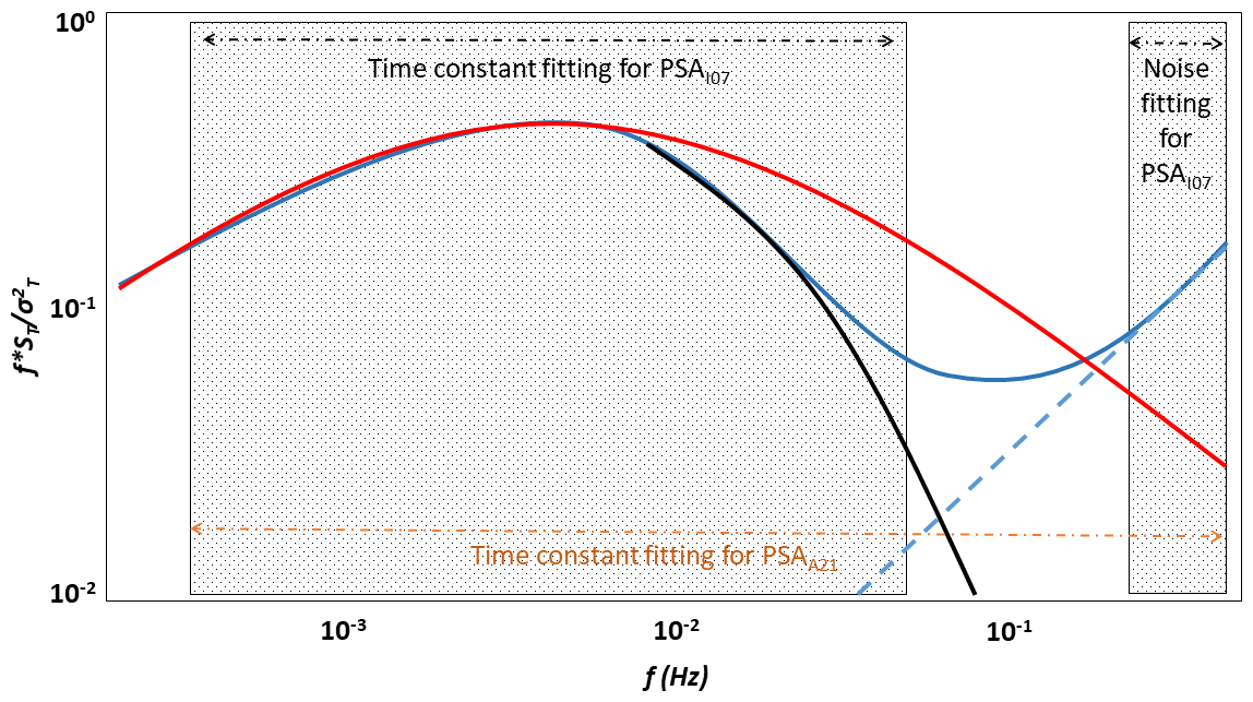
Figure 1 A diagram illustrating fitting procedures for PSA methods. Shown are the spectra of unattenuated and noise-free temperature (red line) and spectra of low-pass filtered and noisy scalar before (solid blue line) and after (black line) noise removal. For PSA_I07, the noise is detected via fitting a line (dashed blue) to the high-frequency end of noisy scalar over the frequency range highlighted. Then, it is extended towards lower frequencies and subtracted from the noisy spectrum, yielding noise-free spectra. Later, the time constant is calculated via fitting Eq. (4) to noise-free spectra over the frequency range highlighted. For PSA_A21, the time constant is obtained from one comprehensive fitting of Eq. (7) to noisy spectra over the whole frequency range highlighted.

3 Materials and methods

3.1 Sites description and measurements

Two datasets measured with sonic anemometer in an EC set-up from the Siikaneva fen site were mainly used in this study. The site is located in southern Finland (61^∘49.9610^′ N, 24^∘11.5670^′ E; 160 m a.s.l.). The data were measured with 10 Hz sampling frequency using a 3-D sonic anemometer (model USA-1; METEK GmbH, Elmshorn, Germany). Further details about the site and measurements can be found in Peltola et al. (2013).

The first dataset (D₁) was used for the time constant calculation (see Sect. 3.2). It contained 70 half-hourly EC data records measured in fully turbulent daytime conditions in the period from May to September 2013 with an average sensible heat flux of 114.3 W m⁻², friction velocity of 0.3 m s⁻¹, and wind speed of 2.1 m s⁻¹.

The second dataset (D₂) was used for the cumulative flux calculation based on T (see Sect. 3.3). This dataset was measured between 1 and 30 May 2013 and consisted of 1440 half-hourly periods for which fluxes were calculated.

Lastly, to demonstrate the performances of different methods in real-world data, we used CO₂ dataset (D₃) measured with 10 Hz sampling frequency using an infrared gas analyser (LI-7000, LI-COR, Lincoln, NE, USA). The measurements were simultaneously done with D₁ at the same set-up at 2.75 m above the peat surface, where the centre of the sonic anemometer was displaced 25 cm vertically above the intake of gas analyser. The air was drawn to the analyser through a 16.8 m long heated inlet sampling line.

3.2 Data processing for time constant estimation

The data processing flow for all variants of PSA and CSA is summarized in Fig. 2. In order to generate the artificial dataset, which represents various known levels of SNR and attenuation, we first applied commonly used EC data processing procedures, i.e. de-spiking, 2-D coordinate rotation of the wind velocity vector, and linear de-trending to D₁. We then degraded each half-hourly T time series with a first order low-pass filter in the spectral domain (see Sect. 3.2.1) and contaminated it with a prescribed amount of white noise in the time domain (see Sect. 3.2.2). For PSA, we calculated power spectra of T, following Sabbatini et al. (2018), normalized it by the total variance calculated within the frequency range of 0.0012 and 0.05 Hz, and averaged it into a logarithmically equally distanced frequency base. Then we took an ensemble average of the 70 power spectra. For PSA_I07, we first removed the noise from the power spectra (see Sect. 2.2), then retrieved the time constant (i.e. ${\mathit{\tau }}_{{\mathrm{PSA}}_{\mathrm{I}\mathrm{07}}}$) via fitting Eq. (4) within a frequency range, the lower limit of which is 0.01 Hz, while the optimal higher limit is defined via visual inspection. For PSA_A21, we obtained the time constant (i.e. ${\mathit{\tau }}_{{\mathrm{PSA}}_{\mathrm{A}\mathrm{21}}}$) via fitting Eq. (4) using the entire frequency domain.

In practice there is no time lag between T and w as both variables are measured with the same instrument. However, low-pass filtering introduces a time lag in the scalar of interest in addition to any physical time lag that may be caused by transport through sampling lines and/or sensor separation (Massman, 2000; Ibrom et al., 2007b; Peltola et al., 2021). In our case, since the scalar of interest is represented by the attenuated T, the time lag occurring between T and w was adjusted via the maximization of the cross-covariance for the time constant estimation in CSA. Next, we calculated cospectra of T and w, normalized them with the total covariance calculated within the frequency range of 0.0012 and 0.05 Hz, and averaged the data into exponentially spaced frequency bins. Then we calculated ensemble averages. Lastly, we derived the time constants for the original dataset (i.e. ${\mathit{\tau }}_{{\mathrm{CSA}}_{\sqrt{\mathrm{H}},\mathrm{sync}}}$) via fitting the square root of Eq. (3). The fit was estimated for the frequency range from 0.01 to 2 Hz.

In summary, for three methods (two PSAs and one CSA), we assessed 45 different conditions each, combining five different attenuation levels with nine different SNRs. We repeated the same procedure 100 times to account for the uncertainty associated with the white noise generation and thus obtained 100 different values for the time constant for all attenuation and SNR levels for both PSA and CSA. The relevant results are shown in Sect. 4.2.

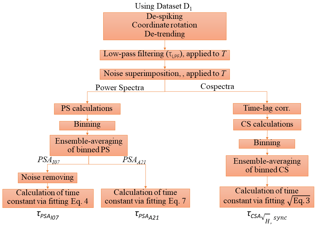
Figure 2 Flow chart of the data processing for time constant calculation using the dataset D₁: τ_LPF is the time constant of the first order filter, ${\mathit{\tau }}_{{\mathrm{PSA}}_{\mathrm{I}\mathrm{07}}}$ and ${\mathit{\tau }}_{{\mathrm{PSA}}_{\mathrm{A}\mathrm{21}}}$ represent the estimated time constants with power spectra (PSA) and ${\mathit{\tau }}_{{\mathrm{CSA}}_{\sqrt{\mathrm{H}},\mathrm{sync}}}$ with cospectra (CSA), and H is the spectral transfer function.

3.2.1 Low-pass filtering

The dynamic performance of any EC measurement system can be approximated with a linear first-order non-homogeneous ordinary differential equation (Massman and Lee, 2002):

$$\begin{array}{}\text{(8)}& {\mathit{\tau }}_{\mathrm{LPF}}{\displaystyle \frac{\mathrm{d}{\mathit{\chi }}_{\mathrm{O}}}{\mathrm{d}t}}+{\mathit{\chi }}_{\mathrm{O}}\left(t\right)={\mathit{\chi }}_{\mathrm{I}}\left(t\right),\end{array}$$

where χ_O is the output of a scalar sensor, χ_I(t) is the true scalar concentration (i.e. input), and τ_LPF is the characteristic time constant of the sensor response (Massman and Lee, 2002). The spectral response (h_LPF(ω)) of such a system can be obtained by the Fourier transform of the ratio of the output signal to the input signal, i.e. ${\mathit{\chi }}_{\mathrm{O}}/{\mathit{\chi }}_{\mathrm{I}}$ (Horst, 1997):

$$\begin{array}{}\text{(9)}& h_{\mathrm{LPF}}\left(\mathit{\omega }\right)={\displaystyle \frac{\mathrm{1}}{\mathrm{1}-j\mathit{\omega }{\mathit{\tau }}_{\mathrm{LPF}}}},\end{array}$$

where ω=2πf and $j=\sqrt{-\mathrm{1}}$.

The desired (i.e. low-pass filtered) output data in the frequency domain can be estimated as

$$\begin{array}{}\text{(10)}& Z_{\mathrm{O}}=h_{\mathrm{LPF}}\left(\mathit{\omega }\right)Z_{\mathrm{I}},\end{array}$$

where Z_I is the Fourier transform of χ_I. From this, the low-pass filtered time series χ_O can be acquired by applying the inverse Fourier transform to Z_O and taking the real part. In practice, the complex conjugate of h_LPF is used to derive the correct temporal lag (scalar lag with respect to w).

We followed this procedure to filter T with five different τ_LPF values, i.e. 0.1, 0.2, 0.3, 0.4, and 0.5 s, corresponding to f_c values of 1.60, 0.80, 0.53, 0.40, and 0.32 Hz, respectively.

3.2.2 Noise superimposition

In this study we use Gaussian white noise, which has equally distributed spectral densities across all frequencies (Stull, 2012), to contaminate the filtered signal in time-space. In order to generate time series with varying levels of SNR, we first generated white noise with unit standard deviation and multiplied the white noise with the standard deviation of the original T time series with different ratios (e.g. from 0.1 to 0.9). This represents the amount of noise compared to the amount of signal (e.g. from 10 % to 90 %). We then added this noise to the filtered signal. As a result, we obtained SNR values of 10.0, 5.0, 3.3, 2.5, 2.0, 1.6, 1.4, 1.2, and 1.1, which are equal to the ratio of the standard deviation of T and the standard deviation of white noise.

3.3 Data processing when estimating long-term budgets

Data processing steps when estimating the long-term budgets using the D₂ dataset are summarized in Fig. 3.

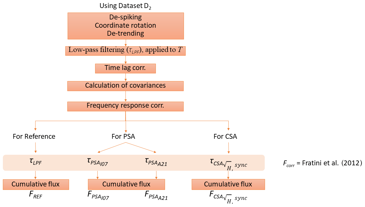
Figure 3 Flow chart of the data processing for the cumulative flux calculation using T of dataset D₂. $F_{{\text{PSA}}_{\mathrm{I}\mathrm{07}}}$, $F_{{\text{PSA}}_{\mathrm{A}\mathrm{21}}}$, $F_{{\mathrm{CSA}}_{\sqrt{H},\mathrm{sync}}}$, and F_REF are the cumulative fluxes corrected by following Fratini et al. (2012), in which F_corr is calculated by implementing the time constants (for PSA: ${\mathit{\tau }}_{{\text{PSA}}_{\mathrm{I}\mathrm{07}}}$ and ${\mathit{\tau }}_{{\text{PSA}}_{\mathrm{A}\mathrm{21}}}$; for CSA: ${\mathit{\tau }}_{{\mathrm{CSA}}_{\sqrt{H},\mathrm{sync}}}$; for reference: τ_LPF) calculated in previous section.

We applied regular EC data processing, which included de-spiking, coordinate rotation, and de-trending. Next, the T time series were deteriorated with values of τ_LPF that varied between 0.1 and 0.5 s to mimic a realistic range of scalar attenuations (mimicking the conditions of, for example, CH₄ or N₂O). Later, the low-pass-induced time lag was accounted for via maximization of the cross-covariance, which was followed by the calculation of the covariances. Then we applied the frequency response correction using Eq. (1), in which F_corr was estimated using the method proposed by Fratini et al. (2012)¹:

$$\begin{array}{}\text{(11)}& F_{\mathrm{corr}}={\displaystyle \frac{\underset{f=f_{min}}{\overset{f_{max}}{\int }}\text{CO}\left(f\right)\mathrm{d}f}{\underset{f=f_{min}}{\overset{f_{max}}{\int }}\text{CO}\left(f\right)\sqrt{H_{\mathrm{emp}}\left(f\right)}\mathrm{d}f}},\end{array}$$

where CO equals the current T cospectrum when the absolute sensible heat fluxes exceeded 15 W m⁻². For small fluxes we used a site-specific cospectral model (see Appendix C) for CO instead of parameterization of F_corr proposed by Ibrom et al. (2007a). To make sure that the analysis was not affected by low data quality, we removed the fluxes with low friction velocity ($u_{*}<\mathrm{0.2}$ m s⁻¹), unrealistic sensible heat fluxes and non-stationary conditions (Foken and Wichura, 1996), eliminating 554 half-hourly data points out of 1440 (ca. 38 %).

The time constant (τ) in H_emp is estimated by either PSA (i.e. ${\mathit{\tau }}_{{\mathrm{PSA}}_{\mathrm{I}\mathrm{07}}}$ and ${\mathit{\tau }}_{{\mathrm{PSA}}_{\mathrm{A}\mathrm{21}}}$) or CSA (i.e. ${\mathit{\tau }}_{{\mathrm{CSA}}_{\sqrt{H},\mathrm{sync}}}$), and this yielded cumulative fluxes $F_{{\mathrm{PSA}}_{\mathrm{I}\mathrm{07}}}$, $F_{{\mathrm{PSA}}_{\mathrm{A}\mathrm{21}}}$, and $F_{{\mathrm{CSA}}_{\sqrt{H},\mathrm{sync}}}$, respectively. For simplicity, in the FRC only median values of time constants of PSA and CSA ensembles estimated were used for each combination of SNR and attenuation. The reference fluxes (F_REF) were also estimated with F_corr using τ_LPF. We present the differences between cumulative fluxes as relative differences with respect to the reference (F_REF) in per cent. In particular, as an example, the relative bias for PSA_I07 is calculated as $\mathrm{100}(F_{{\mathrm{PSA}}_{\mathrm{I}\mathrm{07}}}-F_{\mathrm{REF}})/F_{\mathrm{REF}}$ while for ${\text{CSA}}_{\sqrt{H},\mathrm{sync}}$ as $\mathrm{100}(F_{{\mathrm{CSA}}_{\sqrt{H},sync}}-F_{\mathrm{REF}})/F_{\mathrm{REF}}$ for several attenuation and SNR conditions. The relevant results are shown in Sect. 4.3.

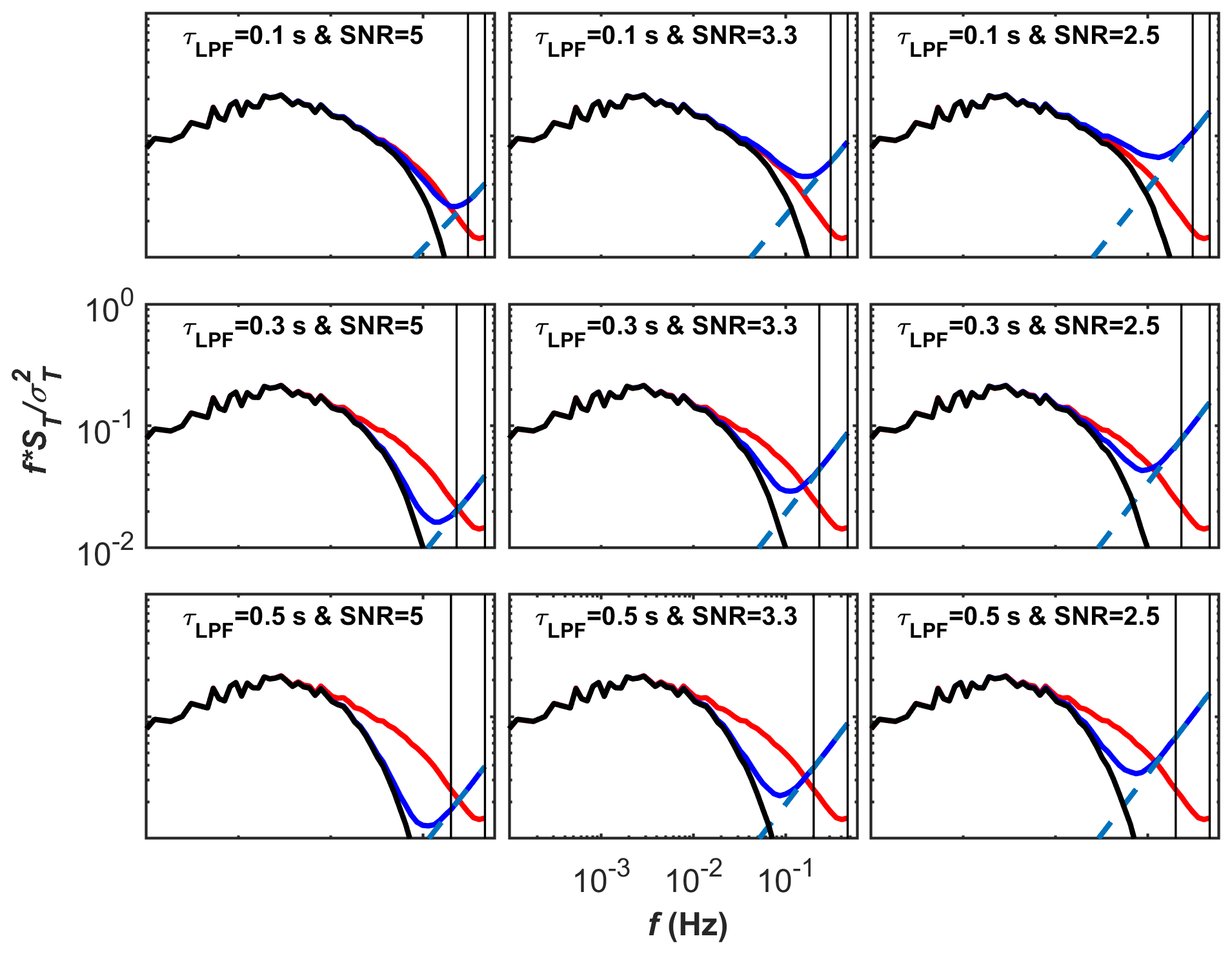
Figure 4 Effect of several low-pass filtering (τ_LPF=0.1, 0.3, and 0.5 s) and SNR (5, 3.3, and 2.5) on spectra of sonic temperature (T) of 70 half-hourly data records illustrated in logarithmic scale, where f is natural frequency, S_T is spectral density, and ${{\mathit{\sigma }}_T}^{\mathrm{2}}$ is the variance of T. Shown are the spectra of raw measured sonic temperature (red lines) and of the artificially deteriorated (i.e. low-pass filtered and noise superimposed) sonic temperature before (dark blue) and after (black) noise removal following Ibrom et al. (2007a) through the subtraction of the linear fit (dashed blue lines) to the high-frequency end of the deteriorated spectra. The vertical lines mark the frequency range used for fitting for noise removal. The lower thresholds of the frequency range are 3, 2.3, and 2 Hz for the attenuation levels of 0.1, 0.3, and 0.5 s, respectively.

4 Results and discussion

4.1 Time constant estimation with PSA

In order to illustrate the important steps in the data analysis in PSA (e.g. low-pass filtering, noise superimposition, and noise removal only for PSA_I07), here we show how the shape of power spectra changes on a logarithmic scale for a few SNR values (5, 3.3, and 2.5) and low-pass filtering conditions (Fig. 4). The low-pass filter time constants (τ_LPF) of 0.1, 0.3, and 0.5 s result in f_c values beyond which the signals become attenuated of ca. 1.6, 0.5, and 0.3 Hz. As the time constant increases, f_c decreases, causing stronger attenuation. Referring to the upper panel of Fig. 4, for constant attenuation (τ_LPF=0.1 s), if the SNR decreases, noise becomes more visible and the line fit to the noise becomes more consistent. Similarly, referring to the left panel of Fig. 4, for constant SNR (e.g. for SNR=5), from top to bottom, as attenuation increases, the slope of the fit increases, and therefore the goodness of fit increases (Table 1). As discussed in Sect. 2.2, white noise causes a slope of 1, and thus any discrepancies from 1 result in overestimated noise removal. Based on Fig. 4 alone, it is evident that removing the noise from power spectra can be done with higher accuracy when the high-frequency attenuation increases and/or SNR decreases.

Table 1 Results of the noise removal procedure applied in the power spectra approach following Ibrom et al. (2007a) (PSA_I07): the values indicate the slopes of the fitted line to the high-frequency end of the spectrum in Fig. 4, with the coefficient of determination (R²) shown in the parenthesis as a function of τ_LPF and SNR. Note that for accurate noise removal the slopes should equal 1.

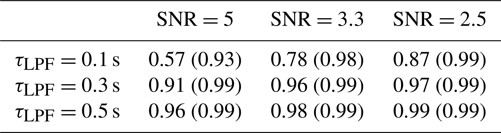
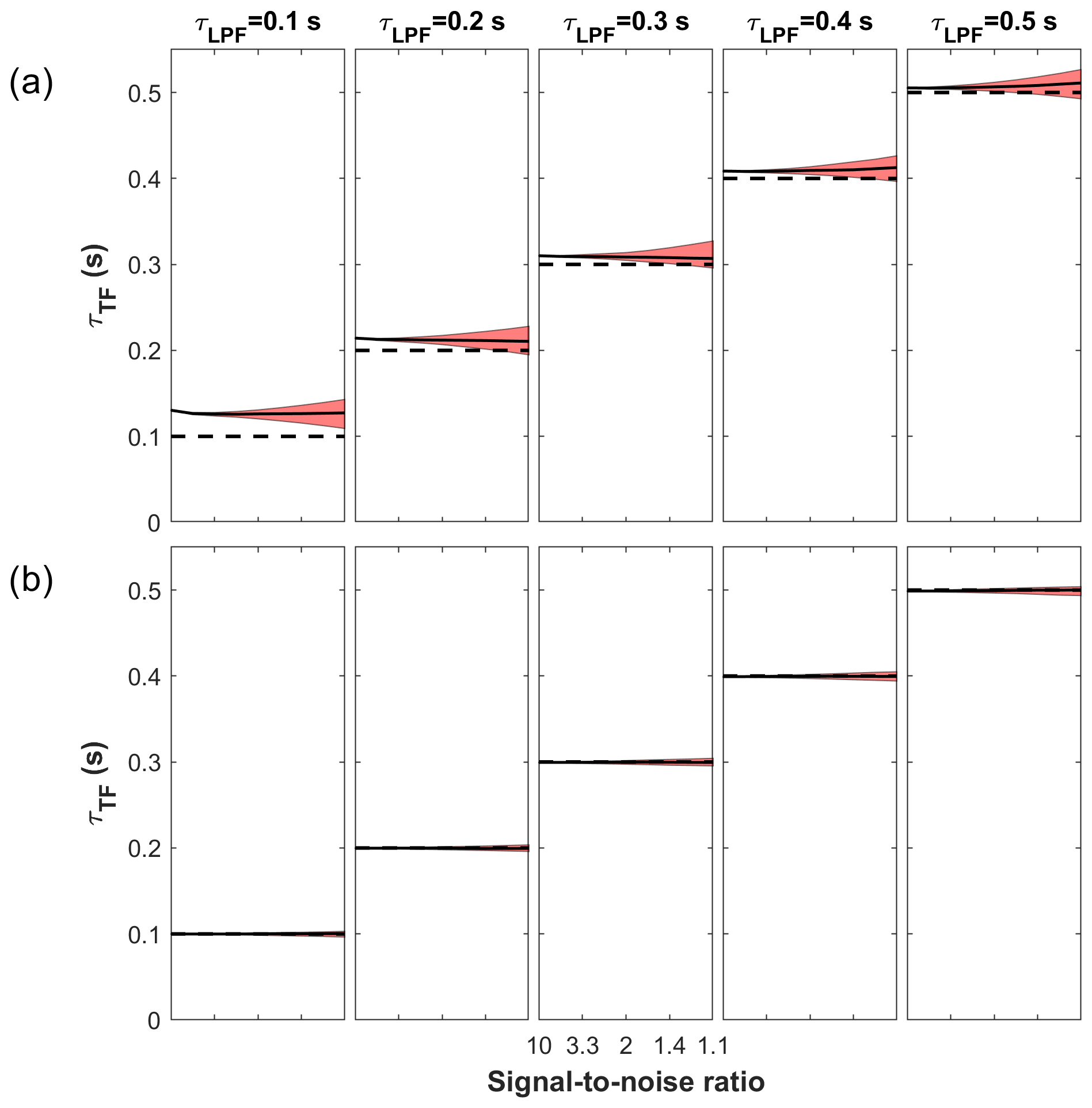
Figure 5 Time constants calculated using the power spectrum approach, comparing (a) PSA_I07 and (b) PSA_A21 in several low-pass filtering conditions (τ_LPF= 0.1–0.5 s) as a function of signal-to-noise ratio (SNR) over the range 10–1.1, which corresponds to the amount of noise (e.g. 10 %–90 %). The solid black curve represents the median, while the shaded area represents interquartile ranges. The dashed line corresponds to the expected value (τ_LPF), which was used for the artificial low-pass filtering.

The results of the time constant estimation are shown in Fig. 5a and 5b for PSA_I07 and PSA_A21, respectively. Results are presented as medians with 25th and 75th percentile ranges for the repeat simulations. It can be seen that for PSA_I07 the interquartile range (IQR) expands as the amount of noise increases, while for PSA_A21 it is small and almost constant with only a slight increase.

For PSA_I07, the optimal frequency domains used for noise fitting were detected as 3, 2.6, and 2.3 to 5 Hz for the different attenuation levels of 0.1, 0.2, and 0.3 s, respectively. For attenuation levels of 0.4 and 0.5 s, we used the frequency range of 2 to 5 Hz.

PSA_I07 overestimates the time constants with improving accuracy from low-attenuation to high-attenuation conditions regardless of the SNR values. The overestimation is likely due to the noise removal procedure, which further attenuates the high-frequency end of the spectra by removing the part of the signal together with noise (i.e. the noise is fitted with a slope <1). In this approach, the accuracy of the noise removal procedure can be improved by visual inspection and adjustment of the fitting range to provide slopes close to 1 and thus better fitting parameters. However, especially for low-attenuation conditions (e.g. 0.1, 0.2 s), the frequency range is not sufficient to detect the noise statistically, meaning that the linear fitting method is not ideal for differentiating in the spectral power the noise contribution from the real variations due to turbulence. In addition to the shortcoming of the linear fitting, the visual inspection of detecting the frequency ranges for both noise removal and the H fitting constitutes another uncertainty source due to its subjectivity. It requires expertise on the topic and is hard to automate when using software used for flux calculations (e.g. EddyPro). Moreover, in some cases, the optimal visual inspection might not be sufficient as the low-attenuation results in our study suggest. In our case we could not further improve the accuracy even though the exact attenuation and SNR level were known, which is not the case with real-world data.

PSA_A21 successfully estimates the time constants regardless of the attenuation and SNR level. This is due to using the whole frequency range for fitting without separating the superimposed attenuated signal and noise. The most important advantage of the PSA_A21 is that it does not require visual inspection.

We assumed that the noise contaminating the signal is white noise, which may not always be the case in real-world data. Thus, the accuracy of the PSA_A21 depends on knowledge of the nature of the noise, which should be determined in advance and implemented in Eq. (6) by adjusting the last term that characterizes the noise. This said, in many EC studies, the type of noise is attributed to white noise (e.g. Launiainen et al., 2005; Peltola et al., 2014; Rannik et al., 2015; Gerdel et al., 2017; Wintjen et al., 2020)² but brown noise in other studies (Wintjen et al., 2020). A simple approach to characterize the type of noise is either by examining the high-frequency end of spectra, which is similar to our study, or through the Allan variance, e.g. Werle et al. (1993). Alternatively, we conducted a brief investigation into the type of noise by comparing the power spectra of measurements with very low SNR and those of white and blue noise (see Appendix B). It should be noted, however, that there are situations when noise is complex and difficult to predict a priori.

4.2 Time constant estimation with CSA

Figure 6 illustrates the time-lag-corrected cospectra of three low-pass filtered cases (i.e. τ=0.1, 0.3, and 0.5 s) with the most noisy conditions (i.e. lowest SNR of 1.1) in addition to the unattenuated and noise-free cospectra (i.e. original). It shows that the white noise contamination did not cause linear increase in the high-frequency end of the cospectra, enabling the time-constant calculation without additional procedure related to noise removal.

${\text{CSA}}_{\sqrt{H},\mathrm{sync}}$ successfully estimates the time constants (Fig. 7). The variation around the expected values can be attributed to the shortcomings in the maximization of the cross-covariance used for the time-lag correction, the precision of which is limited to the sampling interval (e.g. 0.1 s). Hence, the importance of the precision of time-lag detection can be noted as a shortcoming of CSA. The use of square root might be the another reason for the variation as it is an approximation, not an exact representation of the phase shift effect (Peltola et al., 2021).

Lastly, as expected, the level of noise does not affect the accuracy of the CSA method at any SNR level as the random noise does not correlate with w, which is a pivotal advantage of the CSA in general. It does, however, add random noise to the result that is greater than in the improved PSA_A21 approach.

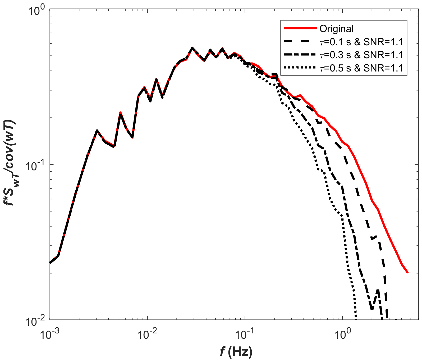
Figure 6 Normalized ensemble cospectra for the original and various attenuated time series (i.e. τ=0.1, 0.3, and 0.5 s). White noise was added at a signal-to-noise ratio (SNR) of 1.1. The red line represents the unattenuated and noise-free cospectrum, while the dashed, dotted-dashed, and dotted lines show the noise-contaminated and low-pass filtered cospectra for the three attenuation levels.

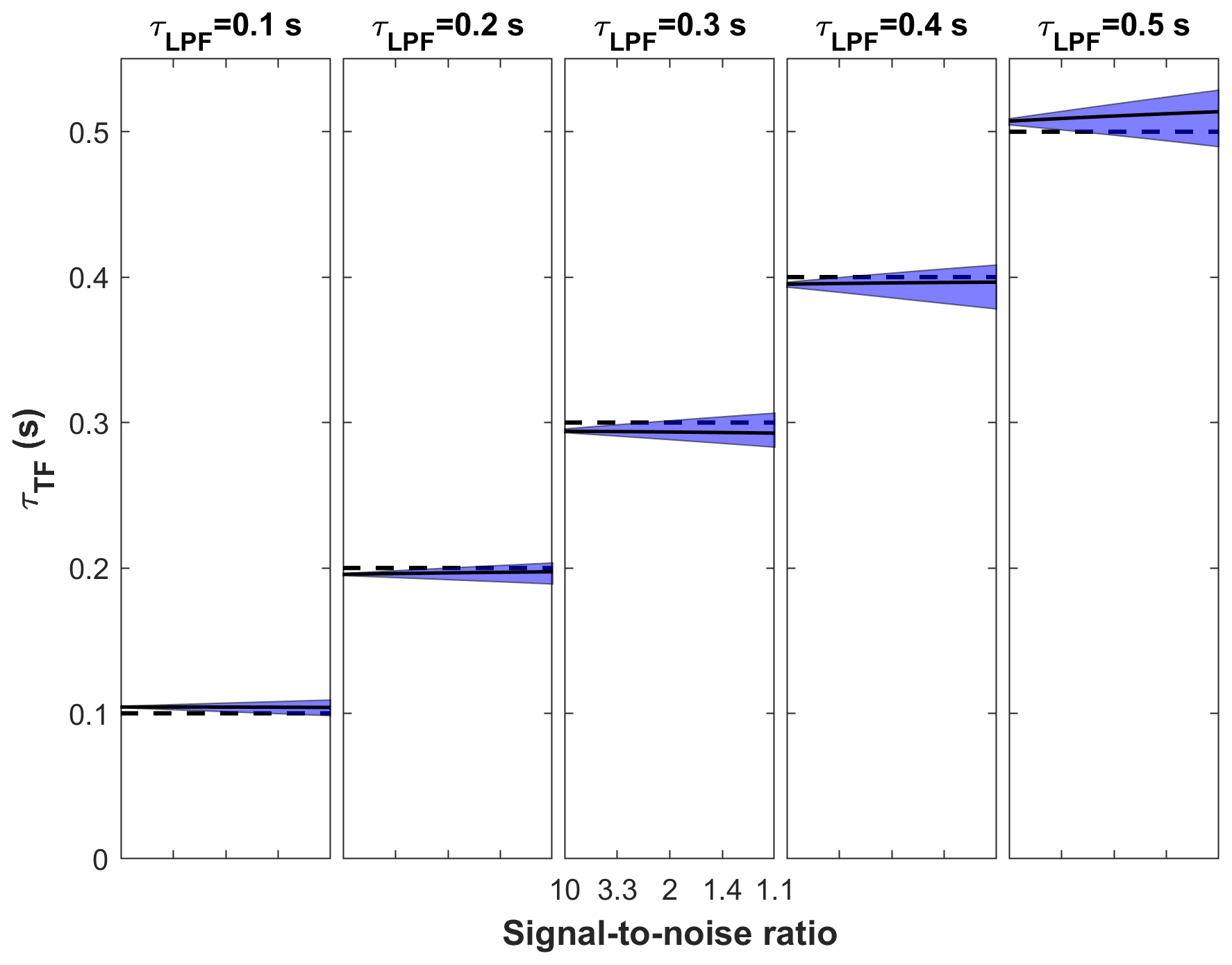
Figure 7 Time constants calculated using the cospectral approach, i.e. ${\text{CSA}}_{\sqrt{H},\mathrm{sync}}$, for several low-pass filtering conditions (τ_LPF= 0.1–0.5 s) as a function of signal-to-noise ratio (SNR) over the range 10–1.1, which corresponds to the amount of noise (e.g. 10 %–90 %). The solid black line represents the medians, while the shaded areas represent interquartile ranges. The dashed line corresponds to the expected value (τ_LPF), which was used for the artificial low-pass filtering.

4.3 Effect of time constant variations on cumulative fluxes

Figures 8 and 9 illustrate how variation in the estimation method of the time constant affected the cumulative fluxes in comparison to reference fluxes (see Sect. 3.3) calculated using dataset D₂. Figure 10 shows the correction factors (F_corr) for the case with τ=0.3 s and SNR of 2. The values vary between 1 and 1.3, indicating the frequency response correction as high as 30 %.

Figure 8 Relative biases of the cumulative fluxes derived with different PSA methods, i.e. PSA_I07 (blue) and PSA_A21 (black), compared with the reference flux as a function of SNR for different attenuation timescales (0.1–0.5 s), calculated as, for example, $\mathrm{100}(F_{{\mathrm{PSA}}_{\mathrm{I}\mathrm{07}}}-F_{\mathrm{REF}})/F_{\mathrm{REF}}$.

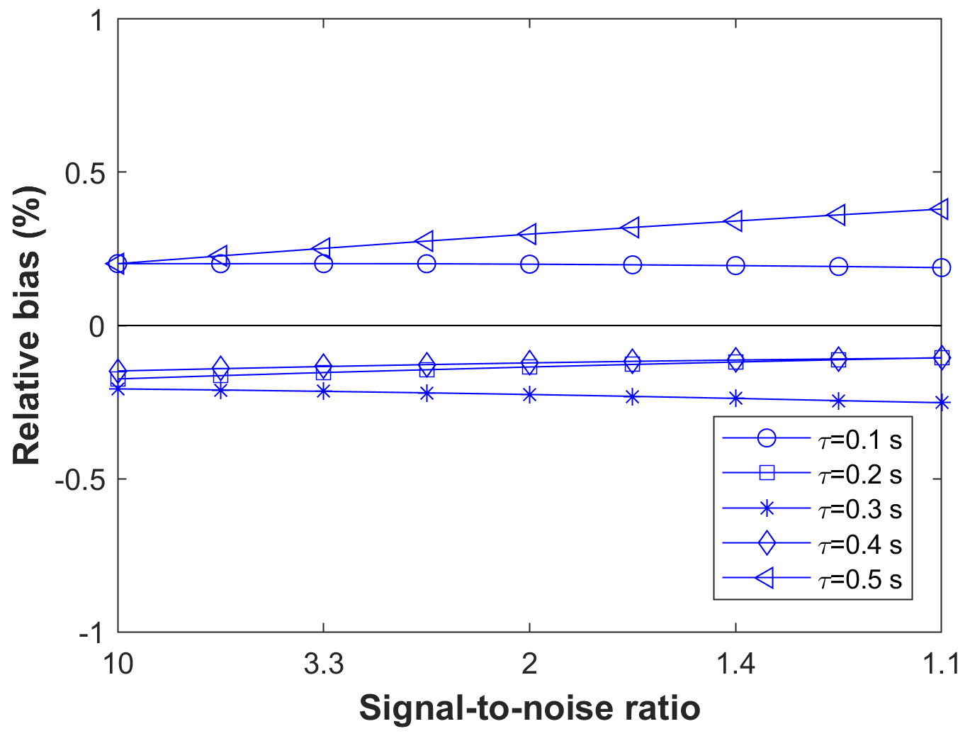
Figure 9 Relative biases of the cumulative fluxes derived with the ${\text{CSA}}_{\sqrt{H},\mathrm{sync}}$ compared with the reference flux as a function of SNR for different attenuation timescales (0.1–0.5 s), calculated as, for example, $\mathrm{100}(F_{{\mathrm{CSA}}_{\sqrt{H},\mathrm{sync}}}-F_{\mathrm{REF}})/F_{\mathrm{REF}}.$

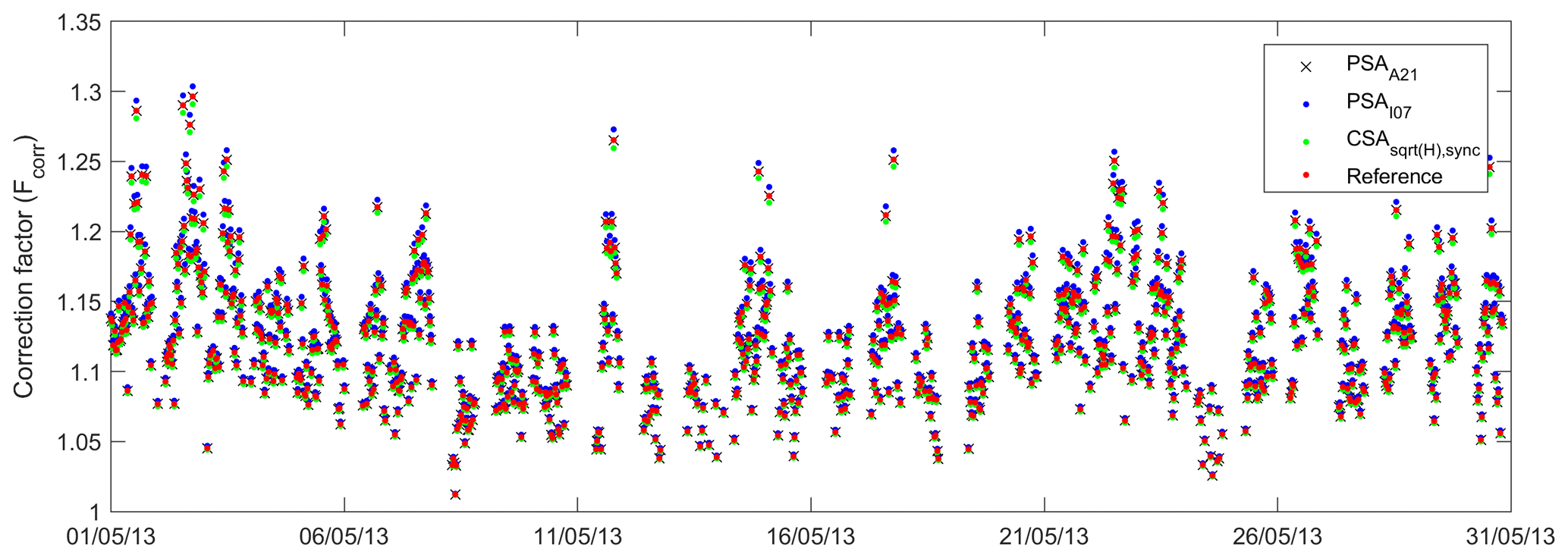
Figure 10 Correction factors (F_corr) of half-hourly fluxes calculated with different approaches, i.e. PSA_A21 (black cross), PSA_I07 (blue point), ${\text{CSA}}_{\sqrt{H},\mathrm{sync}}$ (green point), and the reference (red point) for the case with τ=0.3 s and SNR of 2.

PSA_I07-based fluxes showed a bias varying between 0.1 % and 1.5 %, whereas PSA_A21 showed almost no bias, reflecting the more accurate time constant estimation previously shown. Fluxes based on ${\text{CSA}}_{\sqrt{H},\mathrm{sync}}$ were close to the expected value with the bias of ±0.4 % with negligible response to the SNR level. These findings are consistent with the observed biases in time constant estimation, meaning that where the time constant and the low-pass filtering were overestimated (e.g. with the PSA_I07 especially for τ=0.1 s and ${\text{CSA}}_{\sqrt{H},\mathrm{sync}}$ for τ=0.1 and 0.5 s), the spectral correction factor and thus the fluxes were overestimated, too. In summary, the findings indicate that using the PSA_A21 for the time constant estimation provides quite accurate FRC. On the other hand, for the CSA method, ${\text{CSA}}_{\sqrt{H},\mathrm{sync}}$ reasonably approximates the time constants, hence FRC. These results are in agreement with the analysis presented in Peltola et al. (2021), showing that ${\text{CSA}}_{\sqrt{H},\mathrm{sync}}$ approximates the effect of phase shift on the estimation of the time constant and flux correction factor. See Peltola et al. (2021) for more details.

4.4 Review of typical signal-to-noise ratios and response times encountered during closed-path flux measurements

The range of attenuation and SNR conditions reported in the literature is rather wide and varies depending on ecosystem type, the scalar of interest, data processing, a configuration of instruments, and set-up of the EC system. Ibrom et al. (2007a) examined fluxes of water vapour and CO₂ measured over a temperate forest, both of which were disturbed by noise in the high-frequency range of power spectra (see their Fig. 2). They identified an f_c of CO₂ as low as 0.325 Hz (i.e. ca. τ=0.5 s), indicating strong attenuation, while H₂O showed even stronger attenuation which increased with relative humidity to up to 0.010 Hz (i.e. ca. τ=16 s) due to the sorption/desorption effects on the sampling line internal walls. Langford et al. (2015) reviewed SNR values of various gases published in many studies. In their comprehensive analysis (their Fig. 4), the majority of the half-hourly datasets of isoprene and acetone, measured with a quadrupole-based proton transfer reaction-mass spectrometer (PTR-MS, Ionicon Analytik GmbH, Austria) above broad-leaf woodland, roughly showed SNRs of 0.5 and 0.3, respectively, and benzene measured (with the same instrument) in the urban environment showed an SNR of 0.3. Additionally, N₂O measured with an older tunable diode laser (Aerodyne Research Inc., Billerica, MA, USA) over managed grassland showed an SNR of 1. Rannik et al. (2016) examined the random uncertainties in fluxes measured over forest, lake, and peatland ecosystems in the boreal region. According to their unpublished calculations, the SNRs of CO₂ and H₂O measured with an infrared gas analyser (LI-6262, LI-COR, Lincoln, NE, USA) were 2.6 and 10.3 for the forest site, respectively, while the SNRs of CO₂, H₂O, and CH₄ measured with two closed-path analysers (i.e. LI-7000, LI-COR, Lincoln, NE, USA, for CO₂, H₂O, and FMA, and Los Gatos Research, Los Gatos, CA, USA for CH₄) were 2.7, 24.3, and 5.4, respectively. At the same forest site, Kohonen et al. (2020) investigated fluxes of carbonyl sulfide (COS) with a newer generation Aerodyne quantum cascade laser spectrometer (QCLS) (Aerodyne Research Inc., Billerica, MS, USA) that also measures mole fractions of CO₂ and H₂O. They reported high attenuation for their measurement set-up (time constant of 0.68 s for their EC system) and high noise disturbance in their power spectra (their Fig. 7) with an SNR of about 1. During the measurement period, COS showed small fluxes near the detection limit, causing uncertainty in the calculation of H. Thus, they calculated the time constant using the cospectra of CO₂, assuming that both fluxes are affected by the same attenuation.

In addition, N₂O fluxes measured over urban areas (Järvi et al., 2014) and CO₂ fluxes over lake ecosystems (Mammarella et al., 2015) can also be examples of low SNR conditions.

Given the wide range of SNR and attenuation conditions summarized above, we analysed only a limited range of SNR and attenuation. Also, the impact of the system response time depends on the position of the spectral peak frequency which changes not only with wind speed but also measurement height and surface roughness. Nevertheless, the analysis of the different approaches showed a systematic behaviour with respect to SNR level and attenuation conditions. This provides the opportunity to extend the results of this study beyond the examined values and guides the selection of the right method to find the relevant H.

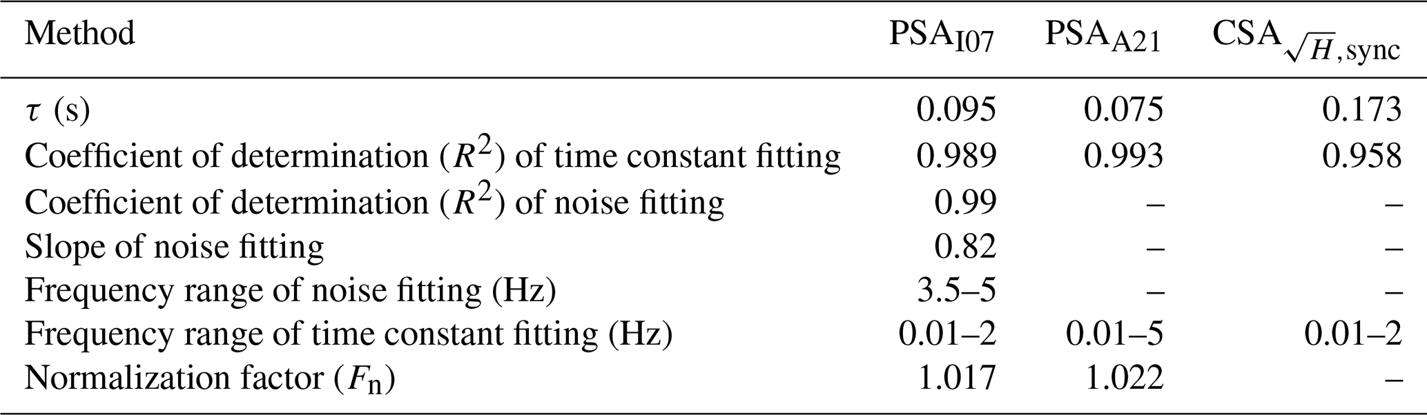
The key constraint of the study was that we artificially simulated the various attenuation and SNR conditions. Thus, demonstrating the performance of the methods with real-world data is of great importance. Accordingly, here we provide an example via processing CO₂ data D₃ with the SNR of 2.3. The power spectra and cospectra of CO₂ and T are shown in Fig. 11. The estimated time constants were 0.095, 0.075, and 0.173 s for PSA_I07, PSA_A21, and ${\text{CSA}}_{\sqrt{H},\mathrm{sync}}$, respectively. The details and statistics of fitting procedures are summarized in Table 2. The PSA_A21 fit successfully approximates the noisy CO₂ power spectra (R²=0.993), enabling us to assume that the noise is white. However, the slope of the linear noise fit of PSA_I07 differs from 1 (0.82). We believe that this is due to the low attenuation so that the noise cannot become visible similarly as in the case of the artificial dataset with low attenuation shown in Fig. 4, resulting in overestimation as it erroneously removes part of the signal together with noise. The differences in time constants obtained via PSA and CSA approaches might be attributed to sensor separation, uncertainties in time-lag correction, and the use of square root in CSA.

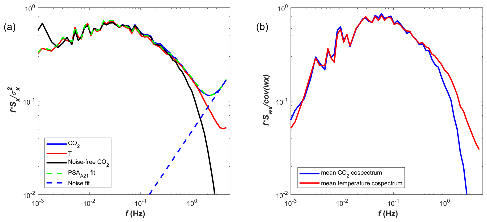
Figure 11 (a) Power spectra of (1) sonic temperature (red), (2) CO₂ from the Siikaneva site measured simultaneously with D₁ (black), and (3) noise-removed CO₂ (dashed blue); shaded areas show the frequency range used for noise fitting for PSA_I07, and time constant fitting for PSA_I07 and PSA_A21. (b) Cospectra of CO₂ (black) and T (red) with vertical wind speed (w).

Table 2 Time constants obtained via different approaches (PSA_I07, PSA_A21, and CSA${}_{\sqrt{H},\mathrm{sync}}$) for CO₂ data from the Siikaneva site and relevant statistics.

5 Conclusions

Here we investigated the limitations of two commonly used approaches to empirically estimate the eddy-covariance (EC) transfer function needed for the frequency response correction of measured fluxes by analysing a temperature flux time series which was synthetically degenerated mimicking slow-response set-ups and noisy sensors. The first approach (PSA) is based on the ratio of measured power spectra, while the second (CSA) is based on the ratio of measured cospectra. For PSA, we examined two alternative approaches of accounting for the white noise contribution to the power spectra: i.e. PSA_I07 and PSA_A21. The latter is newly introduced here and does not require noise removal prior to the fitting of the response function. For CSA, we examined one approach utilizing the square root of the transfer function (H) with shifted w time series via maximization of the cross-covariance, i.e. ${\text{CSA}}_{\sqrt{H},\mathrm{sync}}$. We generated an artificial dataset using T with differing degrees of low-pass filtering (simulated damping) and additional random noise. The advantage of using artificial datasets is that the real values of frequency attenuation, SNR, and physical time lag are all known, allowing the precise comparison of the estimations and expected values. PSA_I07 overestimated the noise contribution and consequently the signal loss and time constant for low-attenuation conditions, but better performance was found as attenuation increases. The new PSA_A21 approach successfully estimated the time constants regardless of the attenuation and SNR level, identifying the noise and signal comprehensively and providing no bias and the lowest random uncertainty in the case of noisy data. However, the approach assumed that the signal is contaminated by white noise, but this is not necessarily always the case. Hence, prior to the calculation of the time constant with this method, the nature of noise must be known. ${\text{CSA}}_{\sqrt{H},\mathrm{sync}}$ showed a slight deviation from expected values. That can be attributed to lack of precision in time-lag estimation and the use of square root.

We then examined the effect of the different approaches to estimate the time constants on the cumulative fluxes: fluxes corrected using the PSA_I07-based time constants showed the bias varying between 0.1 % and 1.5 % in comparison with reference fluxes (see Sect. 3.3), for which PSA_A21 showed almost no bias. By contrast, fluxes corrected using ${\text{CSA}}_{\sqrt{H},\mathrm{sync}}$ showed the bias of ±0.4 %. This analysis, however, does not account for the shortcomings of the method, i.e. Fratini et al. (2012), and thus should be read as the sole effect of time constant estimation on the final fluxes. The comparison of commonly used methods are comprehensively done in the companion paper.

The SNR did not affect the accuracy of either PSA or CSA approaches, alleviating concerns on EC flux measurements with low SNR levels.

In summary, for the empirical estimation of parameters of H of closed-path EC systems, our findings showed that PSA_A21 is the most accurate, precise, and robust method when power spectra are used. This finding was independent of SNR and degree of attenuation. On the other hand, using the square root of H in ${\text{CSA}}_{\sqrt{H},\mathrm{sync}}$, which is a good approximation of the attenuation of cospectra in the presence of phase shifts (Peltola et al., 2021), provided the reasonably correct estimation of τ and F_corr when cospectra are computed after with time-lag quantification by cross-covariance maximization.

Finally, given the constraints of this study, we encourage additional studies based on the real attenuation and SNR conditions, investigating also other types of noise contamination to provide a step forward in efforts to standardize the EC method, which is of great importance to avoid systematic biases of fluxes and improve comparability between different datasets.

Appendix A: Derivation of the PSA_A21

In this section, we derive the new approach for the PSA (i.e. PSA_A21) in detail. We assume that the measured χ contains two independent and additive components: the attenuated turbulent signal and the noise. We further assume that scalar similarity holds (i.e. power spectra of all scalars follow a similar shape). After these assumptions the power spectrum (S_χ) of χ can be written as

$$\begin{array}{}\text{(A1)}& S_{\mathit{\chi }}\left(f\right)={\displaystyle \frac{{\mathit{\sigma }}_{\mathit{\chi }}^{\mathrm{2}}}{{\mathit{\sigma }}_T^{\mathrm{2}}}}H{S}_T\left(f\right)+S_{\mathit{\chi },n}\left(f\right),\end{array}$$

where ${\mathit{\sigma }}_{\mathit{\chi }}^{\mathrm{2}}$ and ${\mathit{\sigma }}_T^{\mathrm{2}}$ are the variances of χ and T related to turbulent signal (no attenuation or noise), S_T(f) is the power spectrum of T, H describes the attenuation of χ due to imperfect instrumentation, and S_χ,n is the noise in the χ measurements. Note that here the noise in the T measurements was neglected as being small except in very low turbulence conditions (when eddy-covariance measurements become problematic anyway and fluxes are removed by the u_* filter). Assuming that the instrument measuring χ can be approximated by a first-order linear sensor and reordering terms, this yields

$$\begin{array}{}\text{(A2)}& {\displaystyle \frac{S_{\mathit{\chi }}\left(f\right)}{{\mathit{\sigma }}_{\mathit{\chi }}^{\mathrm{2}}}}={\displaystyle \frac{S_T\left(f\right)}{{\mathit{\sigma }}_T^{\mathrm{2}}}}{F}_{\mathrm{n}}{\displaystyle \frac{\mathrm{1}}{\mathrm{1}+(\mathrm{2}\mathit{\pi }f\mathit{\tau }{)}^{\mathrm{2}}}}+{\displaystyle \frac{S_{\mathit{\chi },n}\left(f\right)}{{\mathit{\sigma }}_{\mathit{\chi }}^{\mathrm{2}}}},\end{array}$$

where the proportionality constant F_n was introduced due to the effect that noise adds to ${\mathit{\sigma }}_{\mathit{\chi }}^{\mathrm{2}}$ and thus biases the normalization (see Ibrom et al., 2007a). The spectral density is best shown in log–log space as a wide range of frequencies, and spectral densities are well displayed (Stull, 2012), with natural frequency (f) on the x axis and spectral density multiplied by f on the y axis. After multiplication by f, Eq. (A2) becomes

$$\begin{array}{}\text{(A3)}& f{\displaystyle \frac{S_{\mathit{\chi }}\left(f\right)}{{\mathit{\sigma }}_{\mathit{\chi }}^{\mathrm{2}}}}=f{\displaystyle \frac{S_T\left(f\right)}{{\mathit{\sigma }}_T^{\mathrm{2}}}}{F}_{\mathrm{n}}{\displaystyle \frac{\mathrm{1}}{\mathrm{1}+(\mathrm{2}\mathit{\pi }f\mathit{\tau }{)}^{\mathrm{2}}}}+f{\displaystyle \frac{S_{\mathit{\chi },n}\left(f\right)}{{\mathit{\sigma }}_{\mathit{\chi }}^{\mathrm{2}}}}.\end{array}$$

As described in Sect. 2.2, $f\frac{S_{\mathit{\chi },n}\left(f\right)}{{\mathit{\sigma }}_{\mathit{\chi }}^{\mathrm{2}}}$ can be approximated by a model that is linear in frequency in logarithmic space as $f\frac{S_{\mathit{\chi },n}\left(f\right)}{{\mathit{\sigma }}_{\mathit{\chi }}^{\mathrm{2}}}=a\log \left(f\right)+\log \left(b\right)$. In the case of white noise, where a=1, this results in a simplified linear model as $f\frac{S_{\mathit{\chi },n}\left(f\right)}{{\mathit{\sigma }}_{\mathit{\chi }}^{\mathrm{2}}}=\log \left(f\right)+\log \left(b\right)$ and in non-logarithmic space as e^{log (f)+log (b)}, which is fb. Substitution into Eq. (A3) yields

$$\begin{array}{}\text{(A4)}& f{\displaystyle \frac{S_{\mathit{\chi }}\left(f\right)}{{\mathit{\sigma }}_{\mathit{\chi }}^{\mathrm{2}}}}=f{\displaystyle \frac{S_T\left(f\right)}{{\mathit{\sigma }}_T^{\mathrm{2}}}}{F}_{\mathrm{n}}{\displaystyle \frac{\mathrm{1}}{\mathrm{1}+(\mathrm{2}\mathit{\pi }f\mathit{\tau }{)}^{\mathrm{2}}}}+fb.\end{array}$$

It is worth mentioning that this method can be used to retrieve the variance of noise as well since b equals the ensemble-averaged noise power spectra (S_χ,n) divided by ${\mathit{\sigma }}_{\mathit{\chi }}^{\mathrm{2}}$. However, we do not further examine it as it is not the main interest of this study.

Appendix B: Identification of instrumental noise

Here we perform a short analysis to characterize the type of noise in an example high-frequency CH₄ time series by comparing the spectra of a turbulent scalar with those of artificially generated white and blue noise.

Methane fluxes from an upland forest site can be considered to be greatly affected by instrumental noise because fluxes are small and near the detection limit. Therefore, we used a forest methane mixing ratio dataset to identify the type of noise by comparing its spectra with the spectra of white and blue noise which was artificially generated and with the same standard deviation of the methane dataset.

The data were collected at the SMEAR II station (Station for Measuring Forest Ecosystem–Atmosphere Relations), Hyytiälä, southern Finland (61^∘51^′ N, 24^∘17^′ E; 181 m a.s.l.), which is a class 1 Integrated Carbon Observation System (ICOS) ecosystem station. The station is surrounded by extended areas of coniferous forests, and the EC tower is located in a 55-year-old (in 2017) Scots pine (Pinus sylvestris L.) forest with a dominant tree height of 19 m. The measurements were performed with 10 Hz sampling frequency at a height of 23 m, i.e. approximately 4 m above the forest canopy. A fast response laser absorption spectrometer (G2311-f, Picarro, Santa Clara, CA, USA) was used to measure the CH₄ mixing ratio.

Power spectra of methane were calculated using measurements from 10 July at 12:00–14:30 UTC+2. The high-frequency range of the normalized frequency-weighted CH₄ power spectrum follows the f⁺¹ power law scaling, which is consistent with white noise and inconsistent with, for example, blue noise (Fig. B1).

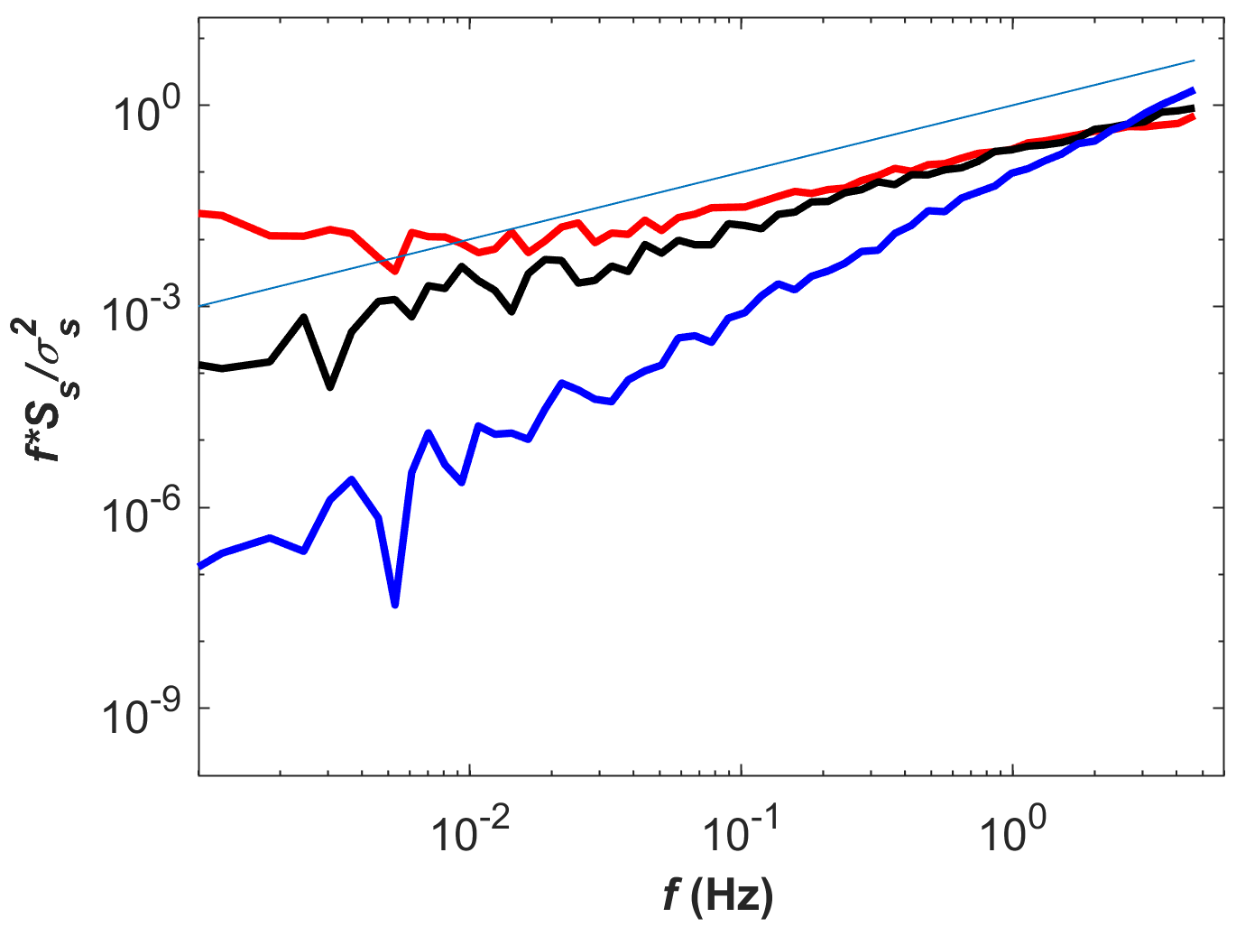
Figure B1 Normalized spectra of methane concentration (red), white noise (black), and blue noise (blue) ($f{S}_{\mathrm{s}}/{\mathit{\sigma }}_{\mathrm{s}}^{\mathrm{2}}$), all of which have the same standard deviation. The solid straight line is f⁺¹ line.

Appendix C: The site-specific cospectral model used in flux calculations

The cospectral model used in flux calculations for small fluxes (i.e. absolute value of sensible heat flux smaller than 15 W m⁻²) was calculated following Horst, 1997:

$$\begin{array}{}\text{(C1)}& {\displaystyle \frac{f\text{Co}\left(f\right)}{\stackrel{\mathrm{‾}}{w^{\prime }{\mathit{\chi }}^{\prime }}}}={\displaystyle \frac{\mathrm{2}}{\mathit{\pi }}}{\displaystyle \frac{n/n_m}{\mathrm{1}+(n/n_m{)}^{\mathrm{2}}}},\end{array}$$

where n is the normalized frequency, and n_m is the cospectral peak frequency, which is derived from in situ measurements in Siikaneva as

$$\begin{array}{}\text{(C2)}& n_m=\left\{\begin{array}{ll}\mathrm{0.09},& \frac{z-d}{L}\le \mathrm{0},\\ \mathrm{0.09}(\mathrm{1}+\mathrm{4.5}(\frac{z-d}{L}{)}^{\mathrm{0.78}}),& \frac{z-d}{L}>\mathrm{0},\end{array}\right.\end{array}$$

where z is the measurement height, d is the displacement height, and L is the Obukhov length, a measure of atmospheric stability.