The high-frequency response correction of eddy covariance fluxes – Part 1: An experimental approach and its interdependence with the time-lag estimation

The eddy covariance (EC) technique has emerged as the prevailing method to observe the ecosystem–atmosphere exchange of gases, heat and momentum. EC measurements require rigorous data processing to derive the fluxes that can be used to analyse exchange processes at the ecosystem–atmosphere interface. Here we show that two common post-processing steps (time-lag estimation via cross-covariance maximisation and correction for limited frequency response of the EC measurement system) are interrelated, and this should be accounted for when processing EC gas flux data. These findings are applicable to EC systems employing closed- or enclosed-path gas analysers which can be approximated to be linear first-order sensors. These EC measurement systems act as low-pass filters on the time series of the scalar χ (e.g. CO₂, H₂O), and this induces a time lag (t_lpf) between vertical wind speed (w) and scalar χ time series which is additional to the travel time of the gas signal in the sampling line (tube, filters). Time-lag estimation via cross-covariance maximisation inadvertently accounts also for t_lpf and hence overestimates the travel time in the sampling line. This results in a phase shift between the time series of w and χ, which distorts the measured cospectra between w and χ and hence has an effect on the correction for the dampening of the EC flux signal at high frequencies. This distortion can be described with a transfer function related to the phase shift (H_p) which is typically neglected when processing EC flux data. Based on analyses using EC data from two contrasting measurement sites, we show that the low-pass-filtering-induced time lag increases approximately linearly with the time constant of the low-pass filter, and hence the importance of H_p in describing the high-frequency flux loss increases as well. Incomplete description of these processes in EC data processing algorithms results in flux biases of up to 10 %, with the largest biases observed for short towers due to the prevalence of small-scale turbulence. Based on these findings, it is suggested that spectral correction methods implemented in EC data processing algorithms are revised to account for the influence of low-pass-filtering-induced time lag.

1 Introduction

The eddy covariance (EC) is the standard micrometeorological technique for measuring vertical turbulent fluxes of momentum, heat and gases in the atmospheric surface layer (Aubinet et al., 2012). Under certain conditions (flat terrain, homogeneous and stationarity turbulent flows, source/sink homogeneity, absence of chemical sources/sinks), the measured EC fluxes represent direct and continuous estimates of the surface exchange of energy and matter between the surface and the atmosphere and are then widely used to estimate energy and water balances, as well as the carbon budget of different type of ecosystems (Baldocchi, 2003; Vesala et al., 2008; Mammarella et al., 2015).

Gas flux measurements are made using a three-dimensional sonic anemometer and a gas analyser, which are able to provide fast-response measurements of turbulent fluctuations of vertical wind velocity and gas concentration (Aubinet et al., 2012). All EC systems, including open-path, enclosed-path or closed-path gas analysers, act as low-pass filters and thus cause a systematic bias to flux estimates. Flux loss at high frequency is due to the incapability of the measurement system to detect small-scale variation. The main reasons for co-spectral attenuation are inadequate frequency response of the sensor, sensor separation and line averaging, as well as, in closed-path systems, the sampling of air through tubes and filters.

The frequency response correction is usually performed based on a priori knowledge of the system transfer function and the unattenuated cospectrum:

$$\begin{array}{}\text{(1)}& \text{CF}={\displaystyle \frac{{\int }_{f_{\mathrm{1}}}^{f_{\mathrm{2}}}{\text{Co}}^{w,\mathit{\chi }}\mathrm{d}f}{{\int }_{f_{\mathrm{1}}}^{f_{\mathrm{2}}}{\text{Co}}^{w,\mathit{\chi }}{H}_{\text{lpf}}\mathrm{d}f}}.\end{array}$$

Here CF is the estimated spectral correction factor, Co^w,χ the normalised unattenuated cospectrum between scalar (χ) and vertical wind speed (w), f the frequency, H_lpf the total transfer function describing the low-pass filtering, and f₁ and f₂ the integration limits that are determined by the length of the averaging period and Nyquist frequency, respectively. The correction, performed by multiplying the measured covariance by the factor CF, always increases the absolute flux magnitude. Note that the high-pass transfer function (Rannik and Vesala, 1999) is not included in Eq. (1) as here we focus only on the low-pass filtering effect of the EC system. The low-pass filtering transfer function H_lpf can be derived either theoretically or empirically (Foken et al., 2012a). The correction is in general different for momentum flux, sensible and latent heat fluxes, and the various gas fluxes and is specific to each EC system. In the theoretical approach, the atmospheric surface layer co-spectral models (Moncrieff et al., 1997) are used, and H_lpf is calculated as a convolution of specific transfer functions representing different causes of flux loss, the equations for which can be found in Moncrieff et al. (1997) and Moore (1986). This approach works well for correcting the fluxes of momentum and sensible heat, as well as gas fluxes measured by open-path systems. Further, Horst (1997) and Massman (2000) have proposed alternative theoretical approaches, providing an analytical estimation of correction factors.

Alternatively, the empirical approach can be used, in which the model cospectra and H_lpf are estimated using in situ measurements. This is the preferable approach for closed-path systems, in which additional effects related to the inlet dust filters and rain caps (Aubinet et al., 2016; Metzger et al., 2016), potential variations in the sampling line flow rate, and absorption and/or desorption processes inside the sampling tube (Ibrom et al., 2007a; Nordbo et al., 2014; Runkle et al., 2012) may contribute to the EC system cut-off frequency, introducing transfer functions which are difficult to estimate a priori.

For this approach, different methods have been proposed for retrieving H_lpf from the measured power spectra or cospectra of the sonic temperature T and the target gas dry mole fraction (Fratini et al., 2012; Ibrom et al., 2007a; Mammarella et al., 2009; Nordbo et al., 2014). While the use of power spectra is the method recommended by the ICOS methodology (Sabbatini et al., 2018; Nemitz et al., 2018) and is implemented in the EddyPro software package, other studies and software packages (EddyUH) have supported the use of measured cospectra (Aubinet et al., 2000; Mammarella et al., 2009, 2016) for the empirical retrieval of H_lpf. The companion paper (Aslan et al., 2021) has investigated methodological issues and flux uncertainty related to these two methods under different attenuation conditions and signal-to-noise ratio scenarios.

In EC systems, particularly those using closed-path gas analysers, the measurements of vertical wind velocity and gas concentration are not co-located, and a time delay between the two signals exists (Aubinet et al., 2012). The standard procedure is to determine this time delay for each averaging period (typically 30 min) by maximising the related cross-covariance function (in absolute terms) and taking the corresponding lag as the true signal delay. However, this time shift between the two signals depends not only on the system set-up (e.g. air sample travel time from the inlet to the infrared gas analyser, IRGA, sampling cell, separation distance between the inlet and the centre of the sonic anemometer path), but it can additionally reflect the low-pass filtering of the measured signal (Massman, 2000; Ibrom et al., 2007a, b).

In this study, we investigate how the low-pass-filtering-induced phase shift affects the estimation of the high-frequency flux loss, and we show the implications that occur when H_lpf time constants are empirically derived from measured power spectra or cospectra and when related CFs values are applied to covariances estimated from the cross-covariance maximum. Finally, we present a method to take the phase shift effect into account when processing EC data. Towards these aims, we use EC data collected above a forest canopy (Hyytiälä) and a wetland (Siikaneva) in Finland covering a large range of attenuation conditions and integral turbulent timescale characteristics.

2 Theory

2.1 Transfer functions

The measured cross-spectrum (Cr_m) between the fluctuations of vertical wind speed and the attenuated and lagged scalar can be described by (e.g. Massman, 2000)

$$\begin{array}{}\text{(2)}& {\text{Cr}}_{\mathrm{m}}=\left[Z_{\mathrm{w}}\right]{\left[h_{\mathit{\chi }}{Z}_{\mathit{\chi }}\right]}^{*}{e}^{-j{\mathit{\varphi }}_{\text{phys}}},\end{array}$$

where Z_w and Z_χ are Fourier transforms of the time series of vertical wind speed (w^′) and scalar (χ^′) fluctuations which are perfectly in phase and not attenuated, h_χ is the Fourier transform of the filter function that describes the response of the instrument measuring the scalar time series, $j=\sqrt{-\mathrm{1}}$, and ϕ_phys=ωt_phys, where t_phys is a constant time shift (s) between w^′ and χ^′ and ω=2πf is the angular frequency, with f representing the frequency (Hz). The superscript ^* denotes complex conjugation. Equation (2) describes the cross-spectra measured with a typical EC system employing a closed-path gas analyser in which the scalar fluctuations are attenuated (h_χ) and delayed in time (t_phys) with respect to w^′ due to the gas sampling system (tubes, filters) and horizontal sensor separation. The signal travel time in the gas sampling line (t_phys) could be approximated from the volume of the sampling line and flow rate. Note that we assume that the sensor measuring w^′ is perfect without any distortions in the measured w^′ time series. This assumption does not limit the generality of the findings below. We also neglect any influence of sensor separation (Horst and Lenschow, 2009) or high-pass filtering on flux attenuation.

Following, for example, Horst (1997) and Massman (2000), the scalar sensor is approximated to be a linear first-order sensor for which h_χ can be written as

$$\begin{array}{}\text{(3)}& h_{\mathit{\chi }}={\displaystyle \frac{\mathrm{1}}{\mathrm{1}-j\mathit{\omega }\mathit{\tau }}},\end{array}$$

where τ is the time constant (s) of the filter, also called response time. Note that $Z_{\mathrm{w}}{Z}_{\mathit{\chi }}^{*}$ is the true cross-spectrum (Cr) between unattenuated w^′ and χ^′ time series which are in phase, and it has a real (cospectrum Co) and an imaginary (quadrature spectrum Q) part (Cr = $Z_{\mathrm{w}}{Z}_{\mathit{\chi }}^{*}$ = Co+jQ). Recall also that the integral of Co equals the unattenuated covariance $\stackrel{\mathrm{‾}}{w^{\prime }{\mathit{\chi }}^{\prime }}$, i.e. the vertical turbulent flux of scalar χ. Following previous studies (Horst, 1997; Massman, 2000), the quadrature spectrum (Q) can be assumed to be zero for stationary turbulent flow and hence Cr = $Z_{\mathrm{w}}{Z}_{\mathit{\chi }}^{*}$ ≈ Co. Now, using Euler's formula and some derivation (see Appendix A), we find

$$\begin{array}{}\text{(4)}& \begin{array}{rl}{\text{Cr}}_{\mathrm{m}}& ={\displaystyle \frac{\cos {\mathit{\varphi }}_{\text{phys}}-\mathit{\omega }\mathit{\tau }\sin {\mathit{\varphi }}_{\text{phys}}}{\mathrm{1}+{\mathit{\omega }}^{\mathrm{2}}{\mathit{\tau }}^{\mathrm{2}}}}\text{Co}\\ & -j{\displaystyle \frac{\sin {\mathit{\varphi }}_{\text{phys}}+\mathit{\omega }\mathit{\tau }\cos {\mathit{\varphi }}_{\text{phys}}}{\mathrm{1}+{\mathit{\omega }}^{\mathrm{2}}{\mathit{\tau }}^{\mathrm{2}}}}\text{Co}\\ & ={\text{Co}}_{\mathrm{m}}+j{Q}_{\mathrm{m}},\end{array}\end{array}$$

where the first term on the right equals the measured cospectrum (Co_m) and the second term the measured quadrature spectrum (Q_m). Note that whilst Q was assumed to be negligible, Q_m is in fact not equivalent to zero even when ϕ_phys=0, i.e. when the travel time of scalar χ^′ signal in the sampling system is zero. This means that w^′ and the attenuated ${\widehat{\mathit{\chi }}}^{\prime }$ (the ^∧ denotes attenuation throughout the text), depending on frequency, can be out of phase due to low-pass filtering of Z_χ with h_χ. This has already previously been noted (e.g. Massman, 2000; Massman and Lee, 2002; Wintjen et al., 2020). Now, simply based on the real part of Cr_m, we can define a transfer function for the first-order system (H) as

$$\begin{array}{}\text{(5)}& H={\displaystyle \frac{\mathrm{1}}{\mathrm{1}+{\mathit{\omega }}^{\mathrm{2}}{\mathit{\tau }}^{\mathrm{2}}}}\end{array}$$

and a transfer function (H_p) for a generic phase shift ϕ as (Massman, 2000)

$$\begin{array}{}\text{(6)}& H_{\mathrm{p}}=\cos \mathit{\varphi }-\mathit{\omega }\mathit{\tau }\sin \mathit{\varphi }.\end{array}$$

These two transfer functions together describe how the measured cospectrum (Co_m) deviates from the cospectrum calculated from ideal measurements free from any attenuation and time shifts (Co).

Similarly, forming the cross-spectrum of the attenuated scalar with itself yields

$$\begin{array}{}\text{(7)}& {\displaystyle }{\text{Cr}}_{\mathrm{m},\mathrm{p}}& {\displaystyle }=\left[h_{\mathit{\chi }}{Z}_{\mathit{\chi }}\right]{\left[h_{\mathit{\chi }}{Z}_{\mathit{\chi }}\right]}^{*}\text{(8)}& {\displaystyle }& {\displaystyle }={\displaystyle \frac{\mathrm{1}}{\mathrm{1}+{\mathit{\omega }}^{\mathrm{2}}{\mathit{\tau }}^{\mathrm{2}}}}{Z}_{\mathit{\chi }}{Z}_{\mathit{\chi }}^{*}=H{Z}_{\mathit{\chi }}{Z}_{\mathit{\chi }}^{*},\end{array}$$

where $Z_{\mathit{\chi }}{Z}_{\mathit{\chi }}^{*}$ is the unattenuated power spectrum. From this it follows that the same transfer function (i.e. H) applies to both power spectrum and cospectrum in the case that there is no phase shift between w^′ and χ^′ (i.e. H_p equals 1) and the quadrature spectrum Q is zero.

2.2 Time-lag determination via cross-covariance maximisation

Ideally the time lag between w^′ and ${\widehat{\mathit{\chi }}}^{\prime }$ would be estimated from the known dimensions of the gas sampling system and flow rate, in addition to other components causing time delay between signals. However, it is in practise difficult to keep track of all the components causing the time delay, and hence a practical (yet sometimes flawed; e.g. Langford et al., 2015) solution has been to estimate the time lag between w^′ and ${\widehat{\mathit{\chi }}}^{\prime }$ via cross-covariance maximisation. This can be considered to be equivalent to finding a time shift t (and hence ϕ=ωt) that maximises the integral of Co_m (i.e. maximises the covariance between w^′ and ${\widehat{\mathit{\chi }}}^{\prime }$).

$$\begin{array}{}\text{(9)}& \underset{\mathrm{0}}{\overset{\mathrm{\infty }}{\int }}{\displaystyle \frac{\cos \left(\mathit{\omega }t\right)-\mathit{\omega }\mathit{\tau }\sin \left(\mathit{\omega }t\right)}{\mathrm{1}+{\mathit{\omega }}^{\mathrm{2}}{\mathit{\tau }}^{\mathrm{2}}}}\text{Co}\mathrm{d}\mathit{\omega }=\stackrel{\mathrm{‾}}{w^{\prime }{\widehat{\mathit{\chi }}}^{\prime }}\left(t\right)\end{array}$$

The original aim of this cross-covariance maximisation is to account for the time lag between the time series w^′ and ${\widehat{\mathit{\chi }}}^{\prime }$ that is induced by sampling lines (air filters, tubing) and horizontal sensor separation, in other words to find such a time lag that removes the $e^{-j{\mathit{\varphi }}_{\text{phys}}}$ term in Eq. (2). After successfully accounting for the travel time (t_phys), the attenuation of the measured cospectrum Co_m (and hence flux) would be described only by H instead of H and H_p (see Eq. 4) since the time-lag estimation sets H_p=1. However, the filter described by Eq. (3) results in a phase shift and hence produces an additional time lag between w^′ and ${\widehat{\mathit{\chi }}}^{\prime }$, i.e. t_lpf. This can be seen from Eq. (4): Q_m differs from zero when ϕ=0 (see also Massman, 2000; Massman and Lee, 2002; Wintjen et al., 2020). Cross-covariance maximisation inadvertently derives the sum of t_phys and t_lpf, which implies that the time lag determined by cross-covariance maximisation is not the desired transport time lag. Using the sum of t_phys and t_lpf instead of t_phys induces a non-negligible negative ϕ in Eq. (4). Hence when shifting the time series according to the cross-covariance maximisation, the transfer function related to the phase shift (H_p) can no longer be neglected and should be calculated using $\mathit{\varphi }=-\mathit{\omega }{t}_{\text{lpf}}$, where t_lpf is the bias in the time lag when estimated via cross-covariance maximisation, in other words the low-pass-filtering-induced time lag (note the minus sign since H_p accounts for the overestimated time lag).

As the maximal possible cospectral energy content per unit frequency can be described with the amplitude spectrum ($A_{\mathrm{m}}=\sqrt{{\text{Co}}_{\mathrm{m}}^{\mathrm{2}}+Q_{\mathrm{m}}^{\mathrm{2}}}$), it can be assumed that after the cross-covariance maximisation (time series shifted by t_phys+t_lpf), Co_m can be approximated by A_m. It is straightforward to derive A_m from Eq. (4):

$$\begin{array}{}\text{(10)}& A_{\mathrm{m}}=\sqrt{{\text{Co}}_{\mathrm{m}}^{\mathrm{2}}+Q_{\mathrm{m}}^{\mathrm{2}}}={\displaystyle \frac{\text{Co}}{\sqrt{\mathrm{1}+{\mathit{\omega }}^{\mathrm{2}}{\mathit{\tau }}^{\mathrm{2}}}}}=\sqrt{H}\text{Co}.\end{array}$$

Hence A_m is attenuated with $\sqrt{H}$ instead of H which describes the attenuation of Co_m in the case that there is no phase shift between w^′ and ${\widehat{\mathit{\chi }}}^{\prime }$ as shown above. This suggests that after cross-covariance maximisation $\sqrt{H}$ approximates HH_p and the correct transfer function for cospectrum calculated after cross-covariance maximisation. However, $\sqrt{H}$ is not equivalent to HH_p. This relates to the fact that Q_m cannot be nullified with a constant time shift since low-pass filtering induces a frequency-dependent time shift ($\frac{\arctan (-\mathit{\omega }\mathit{\tau })}{\mathit{\omega }}$; see Massman, 2000). If Q_m could be nullified, then Co_m=A_m (see Eq. 10) and the attenuation of cospectra could be described accurately with $\sqrt{H}$. Note also that Eq. (10) applies universally, independent of ϕ.

The dependence between low-pass-filtering-induced time lag (t_lpf) and filter response time (τ) was estimated using the approximation $H{H}_{\mathrm{p}}\approx \sqrt{H}$ or $H_{\mathrm{p}}\approx \frac{\mathrm{1}}{\sqrt{H}}$. For this analysis the phase transfer function H_p was approximated by using the series expansion of the terms in H_p (Eq. 6). This approximation resulted in $H_{\mathrm{p}}\approx \mathrm{1}-\frac{\mathrm{1}}{\mathrm{2}}(\mathit{\omega }{t}_{\text{lpf}}{)}^{\mathrm{2}}+\mathit{\omega }\mathit{\tau }(\mathit{\omega }{t}_{\text{lpf}})$. Similarly, $\frac{\mathrm{1}}{\sqrt{H}}$ can be approximated by $\mathrm{1}+\frac{\mathrm{1}}{\mathrm{2}}(\mathit{\omega }\mathit{\tau }{)}^{\mathrm{2}}$. Equating these two approximations up to the second order yields a quadratic equation in which the frequency dependence cancels out: $t_{\text{lpf}}^{\mathrm{2}}-\mathrm{2}\mathit{\tau }{t}_{\text{lpf}}+{\mathit{\tau }}^{\mathrm{2}}=\mathrm{0}$. The solution of this simple equation gives t_lpf=τ. Thus, up to the second-order approximation, which holds roughly up to the frequency value ω=1, the low-pass-filtering-induced time lag equals the time constant of the filter. Note, however, that at this frequency range (ω between 0 and 1) the filtering effect is very weak. The dependence between t_lpf and τ can be determined also by numerically solving $H_{\mathrm{p}}\approx \frac{\mathrm{1}}{\sqrt{H}}$ (which equals $\cos (-\mathrm{2}\mathit{\pi }f{t}_{\text{lpf}})-\mathit{\omega }\mathit{\tau }\sin (-\mathrm{2}\mathit{\pi }f{t}_{\text{lpf}})\approx \sqrt{\mathrm{1}+{\left(\mathrm{2}\mathit{\pi }f\mathit{\tau }\right)}^{\mathrm{2}}}$) and using an assumption that t_lpf is proportional to τ, i.e. t_lpf=Cτ, where C is a proportionality constant. These analyses are continued in Sect. 4.1. Note that the dependency between t_lpf and τ derived here and in Sect. 4.1 was not used in the estimation of correction factors (see Sect. 3.2.1) but merely to analyse the factors controlling the dependency.

3 Materials and methods

3.1 Measurement sites

Measurements from the Siikaneva fen and the Hyytiälä forest site (SMEAR II) were used. Both stations are part of the Integrated Carbon Observation System (ICOS) measurement station network.

The SMEAR II station is situated in southern Finland (61^∘51^′ N, 24^∘17^′ E; 181 $\mathrm{m}\mathrm{a}.\mathrm{s}.\mathrm{l}.$, above sea level). The station is surrounded by extended areas of coniferous forests, and the EC tower is located in a 57-year-old (in 2019) Scots pine (Pinus sylvestris L.) forest with a dominant tree height of ca. 19 m. The EC measurements were performed with 10 Hz sampling frequency at 27 m height, whereas the zero plane displacement height (d) was 14 m. The wind speed components and sonic temperature were measured by a three-dimensional ultrasonic anemometer (Solent Research HS1199, Gill Ltd, Lymington, UK), while carbon dioxide and water vapour mixing ratios were measured by an infrared gas analyser (LI-7200, LI-COR Biosciences, Lincoln, NE, USA). A 0.77 m long tube (4 mm inner diameter) was used to sample air for the gas analyser with a nominal flow rate of 10 L min⁻¹. The centre of the sonic anemometer was displaced 20 cm horizontally and 1 cm vertically from the intake of the gas analyser. The measurement set-up was designed to closely follow the ICOS EC measurement protocols (Franz et al., 2018; Rebmann et al., 2018). The measurements were conducted between May and August 2019.

The Siikaneva fen site is located in southern Finland (61^∘49.9610^′ N, 24^∘11.5670^′ E; 160 $\mathrm{m}\mathrm{a}.\mathrm{s}.\mathrm{l}.$), consisting mainly of sedges (Eriophorum vaginatum, Carex rostrata, C. limosa) and Sphagnum species, namely S. balticum, S. majus and S. papillosum, with a height of ca. 10–30 cm. Further details about the site can be found in Riutta et al. (2007), Peltola et al. (2013) and Rinne et al. (2018). The EC measurements were conducted between May and August 2013. The data used in this study were measured with 10 Hz sampling frequency using a three-dimensional sonic anemometer (Metek USA-1, GmbH, Elmshorn, Germany) and a closed-path analyser (LI-7000, LI-COR Biosciences, Lincoln, NE, USA). The sonic anemometer and the gas inlet were situated 2.75 m above the peat surface, and the air was drawn to the analyser through a 16.8 m long heated inlet sampling line. The centre of the sonic anemometer was displaced 25 cm vertically above the intake of the gas analyser.

A short dataset (hereafter $D_{{\mathrm{S}}_{\mathrm{1}}}$) measured between 09:30 and 11:30 (UTC + 2) on 16 June 2013 at the Siikaneva site was used in the method validation (see Sect. 4.2), whilst long-term datasets from both Siikaneva (hereafter $D_{{\mathrm{S}}_{\mathrm{2}}}$) and Hyytiälä (hereafter D_H) were used to evaluate the accuracy of different spectral correction methods and their effect on CO₂ and H₂O fluxes (see Sect. 4.3).

3.2 Data processing

High-frequency EC data from the two sites were processed in order to evaluate (1) the accuracy of different spectral correction methods and (2) their effect on gas (CO₂ and H₂O) flux estimates at these sites. The processing steps followed commonly accepted routines: (1) data were despiked using a method based on the running median filter (Brock, 1986; Starkenburg et al., 2016), (2) coordinates were rotated using double-rotation which aligned one of the horizontal wind components with the mean wind, setting the mean vertical and cross wind components to zero, (3) gas (CO₂ and H₂O) mole fractions were converted point-by-point to be relative to dry air if not already done internally by the gas analyser (LI-7200), (4) turbulent fluctuations were extracted from the measurements using block-averaging, and (5) time lags between gas or filtered T (see Sect. 3.2.2) and vertical wind time series were accounted for using cross-covariance maximisation. Power spectra and cospectra were calculated after these processing steps. Spectral corrections and the related correction factors (CFs) were calculated using four methods described below; see Sect. 3.2.1. After processing, the flux time series were quality filtered by removing periods with unrealistic sensible heat fluxes or friction velocities and highly non-stationary fluxes (Foken and Wichura, 1996). Site-specific friction velocity thresholds (0.17 and 0.3 m s⁻¹ for Siikaneva and Hyytiälä, respectively) were used to discard gas flux data during low-turbulence periods. Furthermore, at Hyytiälä wind directions between 150 and 230^∘ were discarded since here the mast construction disturbed the airflow. At Siikaneva an omnidirectional sonic anemometer was used mounted on the top of a mast, and hence clearly disturbed wind directions were not identified. After quality filtering 4210 and 4722 30 min periods were available for analysis from Hyytiälä and Siikaneva, respectively.

Atmospheric stability was evaluated using the Obukhov length (L):

$$\begin{array}{}\text{(11)}& L=-{\displaystyle \frac{u_{*}^{\mathrm{3}}}{\frac{v_{\mathrm{k}}g\stackrel{\mathrm{‾}}{w^{\prime }{\mathit{\theta }}_{\mathrm{v}}^{\prime }}}{\stackrel{\mathrm{‾}}{{\mathit{\theta }}_{\mathrm{v}}}}}},\end{array}$$

where u_* is the friction velocity, v_k=0.4 the von Karman constant, g the acceleration due to gravity, and θ_v virtual potential temperature. Overline denotes temporal averaging and primes deviations from the mean. From the Obukhov length, the stability parameter was calculated as $\mathit{\zeta }=\frac{z-d}{L}$, where z is the measurement height and d is the zero plane displacement height.

3.2.1 Empirical estimation of the low-pass filtering of the signal

The total transfer function of an EC set-up can be estimated empirically from measured w–$\widehat{\mathit{\chi }}$ and w–T cospectra:

$$\begin{array}{}\text{(12)}& H_{\mathrm{e},\text{cs}}={\displaystyle \frac{{\text{Co}}^{w,\widehat{\mathit{\chi }}}}{{\text{Co}}^{w,T}}}{\displaystyle \frac{\stackrel{\mathrm{‾}}{w^{\prime }{T}^{\prime }}}{\stackrel{\mathrm{‾}}{w^{\prime }{\widehat{\mathit{\chi }}}^{\prime }}}}{F}_{\mathrm{n}},\end{array}$$

or, alternatively, from the power spectra of the measured scalar and T:

$$\begin{array}{}\text{(13)}& H_{\mathrm{e},\text{ps}}={\displaystyle \frac{S_{\widehat{\mathit{\chi }},\widehat{\mathit{\chi }}}}{S_{T,T}}}{\displaystyle \frac{{\mathit{\sigma }}_T^{\mathrm{2}}}{{\mathit{\sigma }}_{\widehat{\mathit{\chi }}}^{\mathrm{2}}}}{F}_{\mathrm{n}},\end{array}$$

where ${\text{Co}}^{w,\widehat{\mathit{\chi }}}$ denotes the cospectral density between w and $\widehat{\mathit{\chi }}$, and $\stackrel{\mathrm{‾}}{w^{\prime }{\widehat{\mathit{\chi }}}^{\prime }}$ represents the covariance between w and $\widehat{\mathit{\chi }}$. $S_{\widehat{\mathit{\chi }},\widehat{\mathit{\chi }}}$ and ${\mathit{\sigma }}_{\widehat{\mathit{\chi }}}^{\mathrm{2}}$ denote the power spectral density and variance of $\widehat{\mathit{\chi }}$, respectively, and the corresponding terms are defined for T. When estimating H_e,cs and H_e,ps, the covariances and variances were calculated from unattenuated frequencies (between 5 × 10⁻³ and 5 × 10⁻² Hz) (Foken et al., 2012a; Sabbatini et al., 2018). An additional normalisation factor (F_n) was also incorporated in order to take into account the fact that the variances and covariances in Eqs. (12) and (13) may be subject to various high-frequency losses (Ibrom et al., 2007a). Here, w and T were approximated to be free from any low-pass filtering effects, and thus Co^w,T and S_T,T could be used as a reference. H_e,cs and H_e,ps were calculated from ensemble-averaged spectra from measurement periods that fulfilled the following criteria: flux stationarity (Foken and Wichura, 1996) was below 0.3, u_* > 0.1 m s⁻¹, and $\stackrel{\mathrm{‾}}{w^{\prime }{T}^{\prime }}$ > 0.02 K m s⁻¹. For CO₂ it was also required that its turbulent flux was below −0.05 $\mathrm{\mu }\mathrm{mol}{\mathrm{mol}}^{-\mathrm{1}}\mathrm{m}{\mathrm{s}}^{-\mathrm{1}}$, and for H₂O it was required that the flux was directed upwards. For H₂O the transfer functions were determined in relative humidity (RH) bins, and the τ and t_lpf values used in calculating CF were estimated from exponential fits made to the values obtained in the RH bins (similar as for τ in Mammarella et al., 2009). In the case of CO₂ and H₂O fluxes, the power spectra were subjected to noise removal prior to utilising them in Eq. (13) by assuming that the signal was contaminated by white noise and that at the highest frequencies the power spectra contained only noise. See the influence of different noise removal techniques on the estimation of high-frequency attenuation in our companion paper (Aslan et al., 2021).

Often both H_e,cs and H_e,ps are approximated by H with a value for τ that describes the low-pass filtering of the EC set-up according to Eq. (5). Then the measured flux is corrected for low-pass filtering by multiplying it with CF (see Eq. 1). There are different ways to estimate Co^w,χ for Eq. (1). Here we limited the analysis only to periods when the absolute sensible heat fluxes were higher than 15 W m⁻² and estimated Co^w,χ in Eq. (1) with the measured Co^w,T following Fratini et al. (2012).

Sabbatini et al. (2018)Aubinet et al. (2000)Fratini et al. (2012)

Table 1 Methods used in this study to estimate flux losses and related correction factors (CFs) due to low-pass filtering of the scalar signal. See the definitions for H and H_p in Eqs. (5) and (6), respectively. Values for τ (and t_lpf in Method 4) were estimated with non-linear least squares fit to H_e,ps or H_e,cs, in which F_n and τ (and t_lpf in Method 4) were used as fitting parameters. The additional normalisation factor F_n took into account any inaccuracies in estimation of variances and covariances in the calculation of H_e,ps and H_e,cs (Eqs. 13 and 12), respectively. The fits were weighted with temperature cospectra in order to give more weight to frequencies where the scalar fluxes were high.

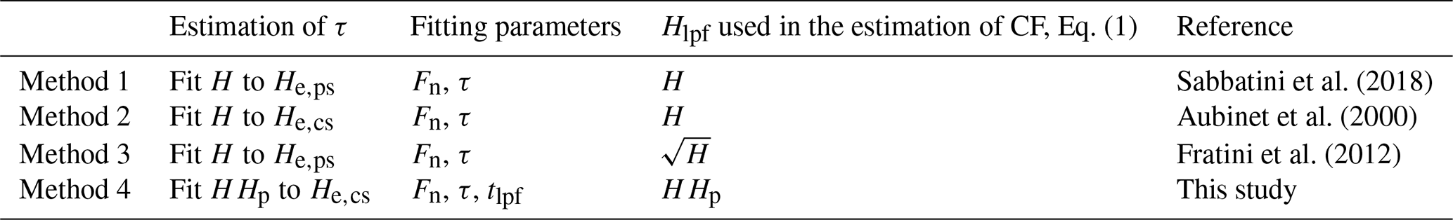
We used four methods to estimate EC system response times (and additionally t_lpf in Method 4) and then to calculate CF (see Table 1). All the four methods are subject to similar limitations; i.e. they are applicable only when the attenuation is not strong at frequencies close to the cospectral peak frequency. Method 1 follows the ICOS EC data processing protocol (Sabbatini et al., 2018) and is implemented, for example, in EddyPro based on Hunt et al. (2016) (see also https://www.licor.com/env/support/EddyPro/topics/whats-new.html, last access: 24 June 2021). Method 2 follows Aubinet et al. (2000) and is implemented in EddyUH (Mammarella et al., 2016). Method 3 follows Fratini et al. (2012) and is implemented in older versions of EddyPro, and Method 4 is the only one that explicitly accounts for the temporal lag caused by the low-pass filtering action of the system and is introduced in this study. In Method 4, both parameters τ and t_lpf, were estimated by fitting HH_p to H_e,cs. Throughout the study, cross-covariance maximisation was used to account for the lag between scalar and vertical wind speed as typically done in the global flux measurement network. Note that also other techniques have been used to estimate the time lag (e.g. Hunt et al., 2016; Taipale et al., 2010) and that the selection of the time-lag estimation method may have an effect on the correct shape of the cospectral transfer function (see Sect. 2). For instance, the cross-covariance moving average method to estimate the time lag introduced in Taipale et al. (2010) should be related to Method 4 as it is also based on cross-covariance maximisation, whereas for the approach in Hunt et al. (2016) the correct cospectral transfer function is H (with the caveat that the physical time lag is estimated accurately).

3.2.2 Low-pass filtering of temperature data

In order to evaluate the performance of the different spectral correction methods presented in Sect. 3.2.1, high-frequency T time series were attenuated with different values of τ in order to mimic attenuated scalar time series. Similar to the procedure used by Aslan et al. (2021), T time series were converted to frequency domain via a Fourier transform, multiplied by Eq. (3) and converted back to time domain with the inverse Fourier transform. Three different values for τ were used: 0.1, 0.3 and 0.7 s. The correct value for CF was obtained from the ratio between $\stackrel{\mathrm{‾}}{w^{\prime }{T}^{\prime }}$ and $\stackrel{\mathrm{‾}}{w^{\prime }{\widehat{T}}^{\prime }}$, where $\widehat{T}$ was the time series attenuated with the methodology described above. Note that here $\stackrel{\mathrm{‾}}{w^{\prime }{\widehat{T}}^{\prime }}$ was calculated using cross-covariance maximisation in order to mimic regular EC gas flux processing, meaning that the lag caused by low-pass filtering was taken into account. This correct value for CF was then compared against CF estimated with the four methods described in Sect. 3.2.1 in order to evaluate the accuracy of the methods.

Figure 1 Top: the value for the proportionality constant C (t_lpf=Cτ) obtained when approximating $H_{\mathrm{p}}\approx \mathrm{1}/\sqrt{H}$ at different frequency ranges. Bottom: H_p and $\mathrm{1}/\sqrt{H}$ calculated using the proportionality t_lpf=0.63τ. See Sect. 4.1 for more details.

4 Results and discussion

4.1 Time-lag dependence on attenuation and turbulence timescales

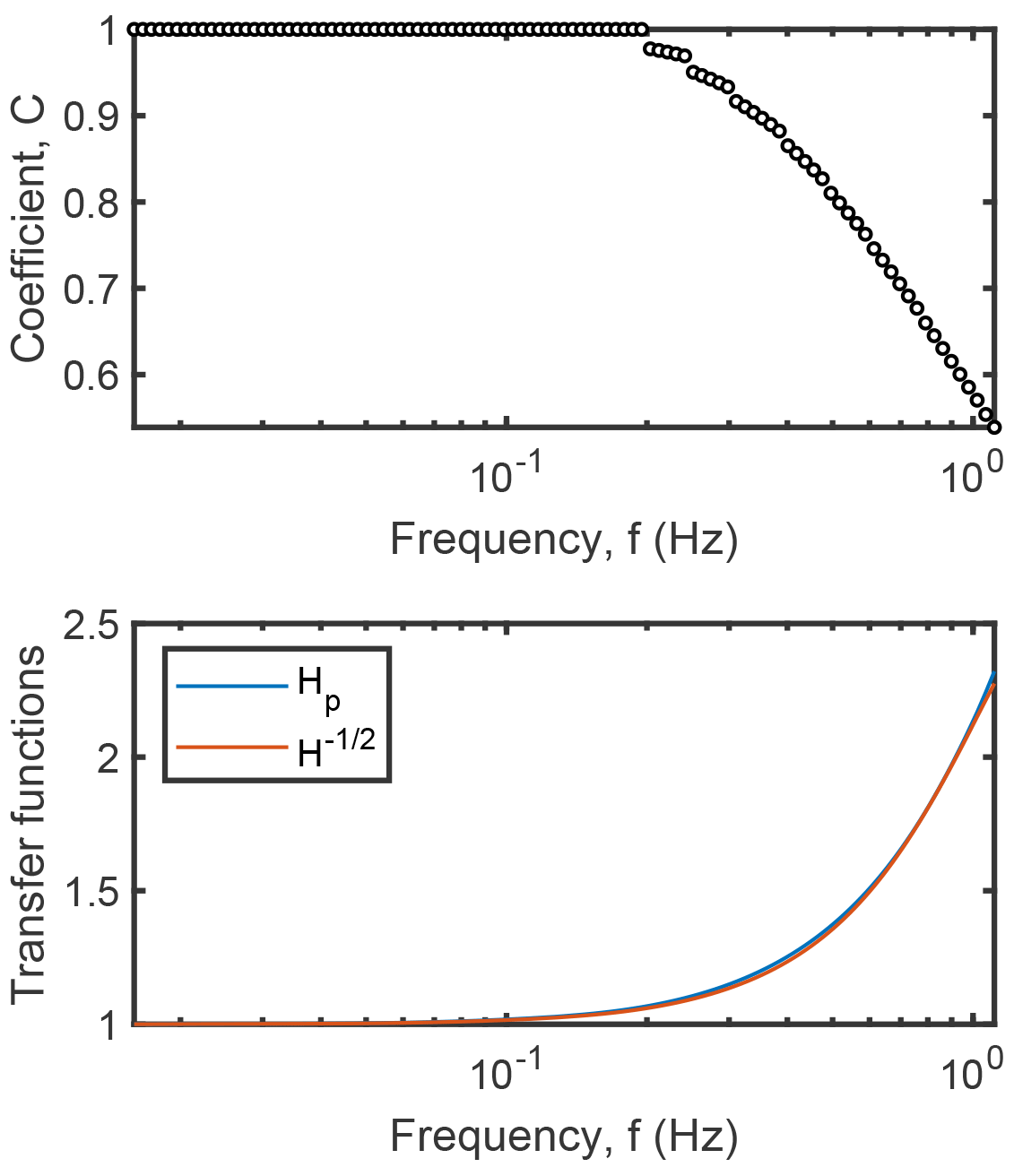
In Sect. 2.2, we explained why the following approximate relationship must hold up to some bound at the high-frequency end: $H_{\mathrm{p}}\approx \mathrm{1}/\sqrt{H}$. Using the assumption that t_lpf=Cτ, this equation was solved numerically for the constant C as a function of frequency f. Figure 1 (upper panel) illustrates that such a solution is dependent on frequency and varies over a relatively large interval up to the frequency $\frac{\mathrm{2}}{\mathrm{3}}\frac{\mathit{\pi }}{\mathit{\tau }}$ (the relationship holds well up to such a frequency for any τ). This suggests that t_lpf and τ are not directly proportional, but their relation depends on frequency. In accordance with the approximations with the Taylor expansion (Sect. 2.2), at low frequencies the constant C equals 1. For illustration, the lower panel of Fig. 1 presents the left and right side terms of the approximate equality ($H_{\mathrm{p}}\approx \mathrm{1}/\sqrt{H}$) calculated using a value of 0.63 for the coefficient C. In spite of the large variation of the exact coefficient with frequency shown in the upper panel in Fig. 1, the selected constant value produces very good correspondence for the whole frequency range, suggesting that C can be approximated to be constant, although strictly speaking it is not. The value of C=0.63 was obtained by estimating the average time lag in a least square sense over equally spaced frequencies in logarithmic scale over the interval from $\mathit{\tau }=\mathrm{0.01}\frac{\mathit{\pi }}{\mathit{\tau }}$ to $\frac{\mathrm{2}}{\mathrm{3}}\frac{\mathit{\pi }}{\mathit{\tau }}$ for a range of time constants from 0.05 to 1 s. We observed that the optimum coefficient was independent of τ and equal to 0.63 (with two-digit accuracy). Note that these analyses were independent of the actual turbulent signal as they were obtained using the transfer functions only (H and H_p).

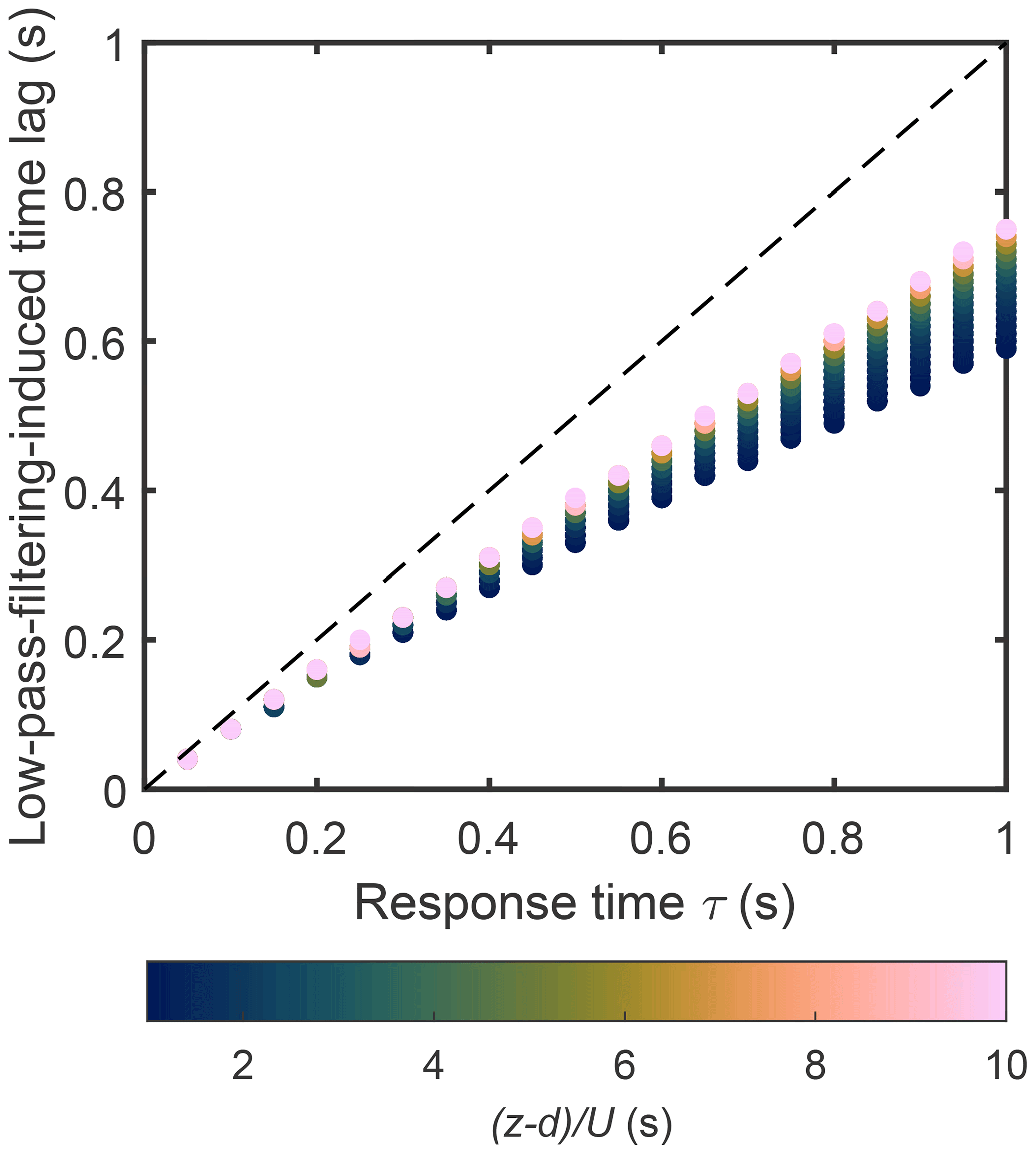
Figure 2 Low-pass-filtering-induced time lag (t_lpf) plotted against response time (τ). The t_lpf values were estimated by numerically integrating the integral in Sect. 2.2 with various time-lag values and evaluating which value resulted in maximum value for various τ and $(z-d)/U$ combinations. The dashed line shows 1:1 correspondence. See Sect. 4.1 for more details.

In order to evaluate the influence of turbulent signal on the dependence between t_lpf and τ, the integral in Sect. 2.2, i.e. Eq. (9), was solved numerically with various combinations of time lag, τ and $(z-d)/U$ in order to evaluate which time-lag value resulted in maximum value for the integral for a given τ and $(z-d)/U$ combination. This approach is similar to finding the time lag between signals using cross-covariance maximisation, and it identified the dependence of the low-pass-filtering-induced lag (t_lpf) on τ and the turbulence timescale ($(z-d)/U$). For this numerical experiment, τ varied between 0.05 and 1 s, $(z-d)/U$ between 1 and 10 s, and Co was calculated based on a model (similar to the one in Kristensen et al., 1997, but fitted to Siikaneva observations). Based on this analysis, t_lpf depended approximately linearly on τ (Fig. 2) in accordance with the analysis above, yet the dependence had an additional weak $\frac{\mathit{\tau }U}{z-d}$ term: $t_{\text{lpf}}=a\mathit{\tau }-b\frac{\mathit{\tau }U}{z-d}+c$, where a=0.73, b=0.15 s and c=0.02 s. However, this numerical experiment was repeated also for very high-attenuation levels; the dependence found above failed to fully recover t_lpf values at high attenuation, and this bias increased with τ and inverse of turbulence timescale (i.e. $U/(z-d)$). For example at τ=2 s and $(z-d)/U=\mathrm{1}\mathrm{s}$ the equation above gave t_lpf=1.2 s, whereas based on the numerical integration value 1.0 s was obtained, meaning that the dependence above was not able to accurately describe the low-pass-induced time lag at these high-attenuation levels. This is likely due to the fact that also the shape of the cospectrum Co in Eq. (9) has an effect on t_lpf dependence on τ. At very high-attenuation levels the peak of the cospectrum is also attenuated, and this results in a different t_lpf dependence on τ than the equation above which describes the dependence when attenuation takes place at high frequencies (i.e. inertial subrange).

The discrepancy between the two dependencies between t_lpf and τ obtained above was likely due to the fact that the latter took into account also the variability in the turbulent flux with frequency, whereas the former was based purely on transfer functions. Nevertheless, these results indicate that, for a given site, t_lpf can be approximated to be constant at a specific attenuation (τ) level, hence supporting the estimation of t_lpf as a fitting parameter in Method 4 when fitting HH_p to H_e,cs (see Sect. 3.2.1 and Table 1).

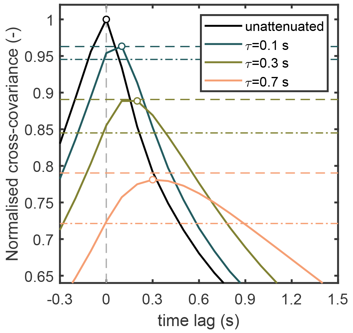
Figure 3 Cross-covariance between w and $\widehat{T}$ calculated from data measured between 09:30 and 11:30 on 16 June 2013 at the Siikaneva site. T data were attenuated with Eq. (3) and three different values for τ in order to demonstrate the effect of filtering on cross-covariance. All the cross-covariance values were normalised with a maximum of unattenuated cross-covariance (i.e. unattenuated covariance). Dots highlight the maxima. Horizontal dashed lines show the attenuation factor (inverse of correction factor, $\mathrm{1}/\text{CF}$) values calculated with Method 4, and dash-dot lines show the attenuation factors calculated with Method 1. Note that the dash-dot lines match the cross-covariance values at zero lag, whereas dashed lines agree with the cross-covariance maxima.

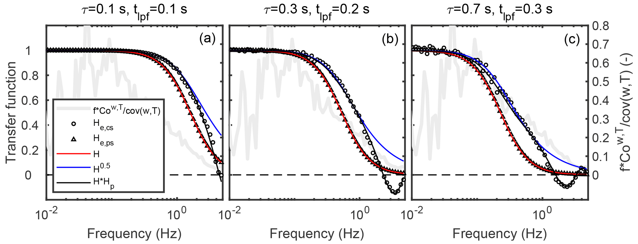
Figure 4 Transfer functions (left y axes) and frequency-weighted and normalised cospectrum (right y axes) for the same data shown in Fig. 3. Note that here H, $\sqrt{H}$ and HH_p were not fitted but calculated using the known values for τ and t_lpf resulting from the low-pass filtering of the T time series (Sect. 3.2.2). Nevertheless, H is related to Method 1, H^0.5 to Method 3 and HH_p to Method 4 (see Table 1). Note also that the cospectrum shown in the figure was calculated from the unattenuated T time series in order to demonstrate the frequency range making the biggest contribution to the flux.

4.2 Assessment of the flux loss correction methods using an attenuated T time series

The four methods to estimate the CF (Table 1) were evaluated using an artificially attenuated turbulent T time series comparing different values for τ. Figure 3 shows example cross-covariance functions from the Siikaneva site with three different values of τ applied to the same 2 h time series.

The peak of the cross-covariance between w and $\widehat{T}$ shifted to longer positive times (i.e. $\widehat{T}$ lags w), and the cross-covariance maximum decreased as τ increased. This is related to the phase shift and flux attenuation caused by the low-pass filter, respectively. The low-pass filtering was also evident in the corresponding power spectra and cospectra. The resulting empirical transfer functions in Fig. 4 show that power spectra were more attenuated than the cospectra when cospectra were calculated from data in which the time lag derived from cross-covariance maximisation was used to shift the time series (as is typically done when processing EC data). Moreover, the shape of the empirical transfer function derived from the cospectra differed from Eq. (5). This difference in shape was related to H_p and the phase shift caused by the low-pass filter. Note that the phase shift resulted in negative values for HH_p and H_e,cs at high frequencies, meaning that the related attenuated cospectrum had both positive and negative values. This implies that attenuated cospectra should not be presented on log–log scales (negative values cannot be presented on log scale). Note also that HH_p is not exactly equal to $\sqrt{H}$ at all frequencies. In particular, HH_p shows negative values at high frequencies, whereas $\sqrt{H}$ does not. Hence the approximation of HH_p with $\sqrt{H}$ will likely fail under very strong attenuation. When the correction factor was calculated with Method 4, which takes into account the low-pass-filtering-induced phase shift, the attenuation factors ($\mathrm{1}/\text{CF}$) agree with the normalised cross-covariance maxima (see Fig. 3). This indicates that the attenuation of cross-covariance maxima was accurately estimated with this method. However, when H_p was neglected and the attenuation factors were calculated with H only, then they agreed with cross-covariance values at zero lag like those predicted by theory (Sect. 2). Note that the time lag discussed here only represents the low-pass-filter effect and not other effects that also alter the time lag. This is only possible because we work with degraded temperature time series, in which phase shifts through low-pass filtering are the only cause for time delays.

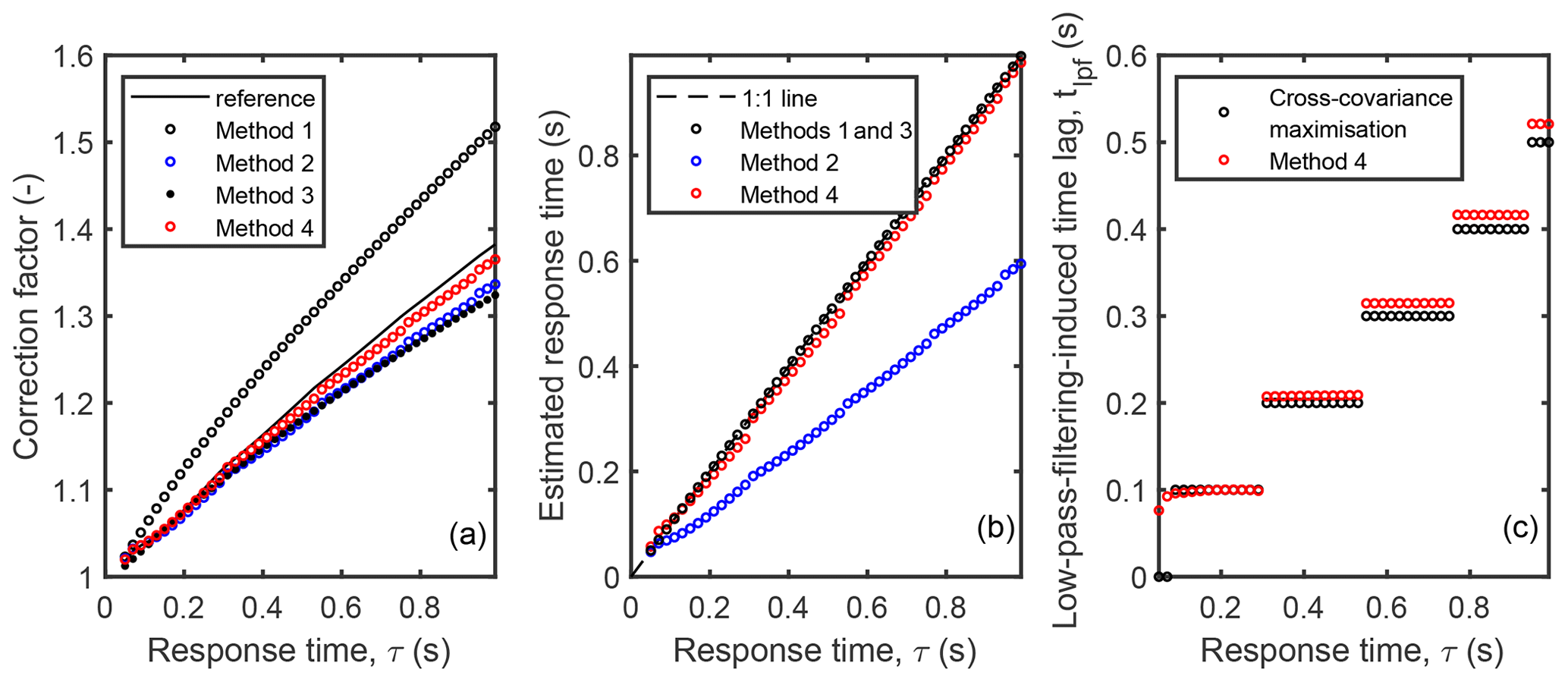
Figure 5 Comparison of estimated correction factors and response times to the values used to attenuate the T time series. The reference values for the correction factors were calculated as the ratio between $\stackrel{\mathrm{‾}}{w^{\prime }{T}^{\prime }}$ and $\stackrel{\mathrm{‾}}{w^{\prime }{\widehat{T}}^{\prime }}$, where $\widehat{T}$ is the temperature time series attenuated according to Sect. 3.2.2. Note that $\stackrel{\mathrm{‾}}{w^{\prime }{\widehat{T}}^{\prime }}$ was calculated using cross-covariance maximisation. The time lags obtained from cross-covariance maximisation and from fitting HH_p to H_e,cs are shown in panel (c). The same data were used as in Figs. 3 and 4.

The value for τ used in attenuating the T time series was further varied between 0.05 and 1 s and used for the same 2 h time series. The bias in CF calculated with Method 1 increased with τ (Fig. 5a). The other methods did not produce as significantly biased estimates for CF when using this example dataset, although methods 2 and 3 somewhat underestimated CF (approximately 4 % underestimation when τ = 0.9 s), and this underestimation increased with τ. These findings are in agreement with Fig. 4: $\sqrt{H}$ was above and H below the empirical transfer function calculated from the cospectrum (H_e,cs), meaning that they underestimated and overestimated the attenuation, respectively. These findings are also in accordance with the results of Aslan et al. (2021) with noisy measurements. Note that Method 2 estimated close to correct value for CF (Fig. 5a) despite biased estimates for the response time (Fig. 5b) due to the compensation of two errors (biased τ and incorrect shape for the cospectral transfer function). Method 4 was able to reproduce the correct value for τ from H_e,cs (Fig. 5), indicating that the difference between H_e,cs and H_e,ps was indeed related to H_p and the low-pass-filtering-related phase shift. The time lags estimated by Method 4 (i.e. by fitting HH_p to H_e,cs) agreed with the ones estimated by maximising the cross-covariance (Fig. 5c), also corroborating this conclusion. It should be noted that the step changes in the data that are very visible in Fig. 5c but to some extent also in Fig. 5a and b are caused by the finite resolution of the underlying data of w and T of 0.1 s.

Table 2 Relative difference between the mean sensible heat fluxes obtained with the different correction methods ($\left(\text{cor-ref}\right)/\text{ref}\cdot \mathrm{100}\mathit{\%}$) and the reference (unattenuated sensible heat flux). All values are in per cent (%).

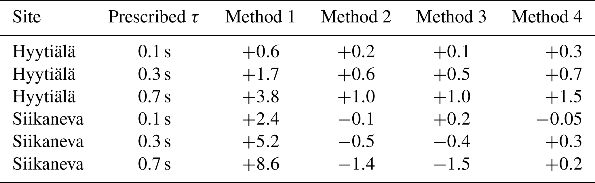
In order to evaluate the four methods to estimate CF further, turbulent T data were low-pass filtered with three values of τ (0.1, 0.3 and 0.7 s) over several summer months (May–August) at two contrasting EC sites, Hyytiälä and Siikaneva. Then the related flux attenuation was corrected with the four methods, and the results were compared against a reference flux calculated from unattenuated T data. Table 2 summarises the relative differences between the four correction methods and the reference. In general, the values obtained with this extended dataset are in line with Fig. 5a for Siikaneva, although slight differences can be noted. The performance of all four methods decreases with increasing τ at both sites, and Method 1 showed the worst performance, which is in line with the example shown in Fig. 5 and follows the predictions from theory (Sect. 2). Of the analysed cases, the biggest bias (+8.6 %) was found when applying Method 1 at Siikaneva with τ = 0.7 s. In general, the performance of the methods was worse at Siikaneva than at Hyytiälä. This was likely related to the lower measurement height at Siikaneva (z−d = 2.7 m) than at Hyytiälä (z−d = 13 m) and thus the comparably larger contribution of high frequencies to the covariance. At Siikaneva, smaller eddies dominated the turbulent transport, and hence the effect of inaccuracies in describing the high-frequency attenuation of the signal was amplified compared with Hyytiälä.

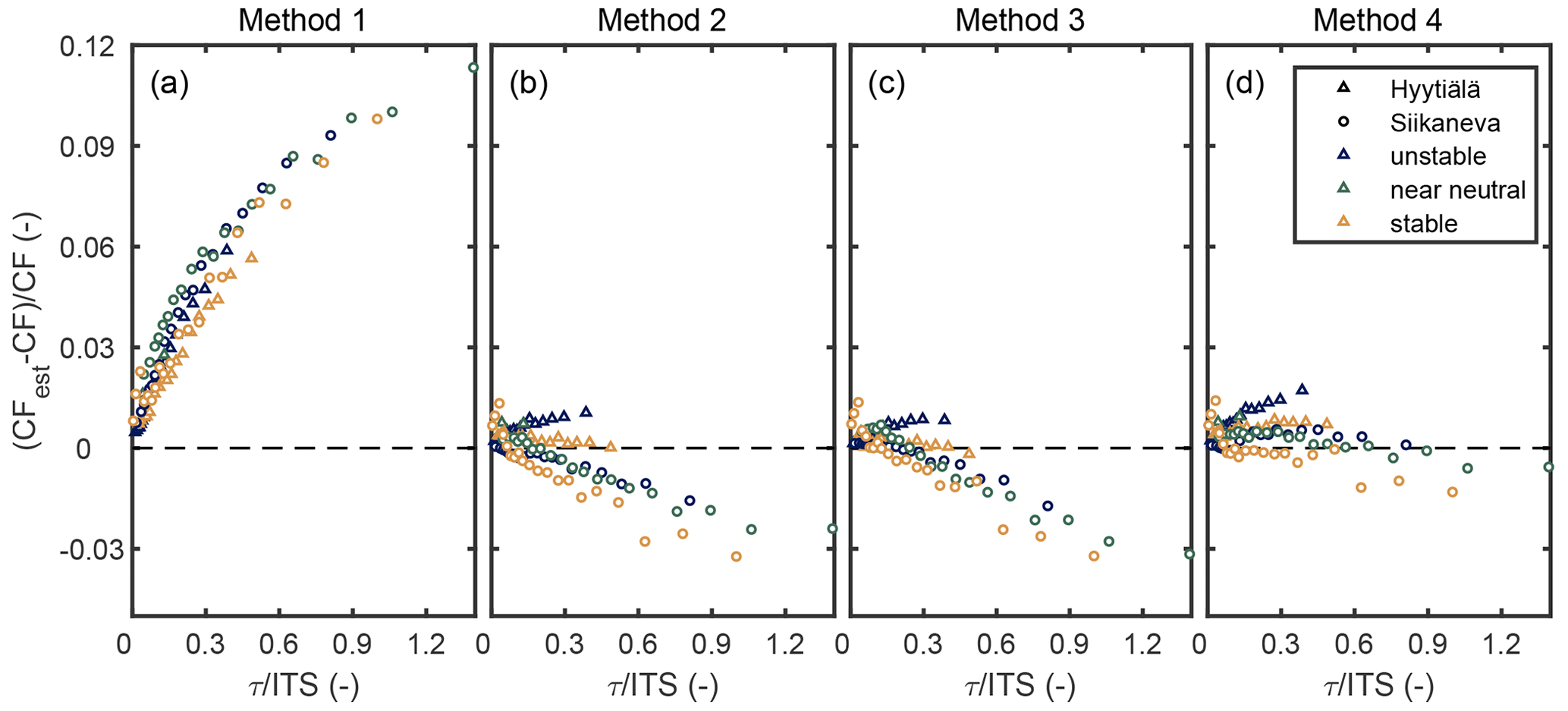
Figure 6 Relative bias in the estimated correction factor (CF_est) against $\mathit{\tau }/\text{ITS}$, where ITS is the integral timescale of $w^{\prime }{T}^{\prime }$. Data were divided into unstable ($\mathit{\zeta }<-\mathrm{0.1}$), stable (ζ>0.1) and near-neutral (|ζ|<0.1) cases before bin-averaging and plotting. Reference values for the correction factor (CF in the figure) were calculated from the ratio between unattenuated and attenuated covariances. Note that the different colours refer to different stability conditions and markers to the different sites.

The importance of turbulence scale on the performance of the four methods was evaluated by stratifying the data according to stability and plotting them against $\mathit{\tau }/\text{ITS}$ (Fig. 6), where ITS is the integral timescale of $w^{\prime }{T}^{\prime }$ calculated from the autocovariance of $w^{\prime }{T}^{\prime }$ time series by integrating the normalised autocovariance function until its first zero crossing (e.g. Kaimal and Finnigan, 1994). This ratio describes the ratio of attenuation and turbulent transport scales. It is also worth noting that this ratio can alternatively be approximated by the ratio of the cospectral peak frequency ($f_m=n_{\mathrm{m}}U/(z-d)$, where n_m is the normalised cospectral peak frequency) to the cut-off frequency ($f_{\text{co}}=\mathrm{1}/\left(\mathrm{2}\mathit{\pi }\mathit{\tau }\right)$) (Rannik et al., 2016). High values for $\mathit{\tau }/\text{ITS}$ describe periods when the attenuation timescale is large relative to the timescale of turbulent scalar transport, whereas low values correspond to cases when the attenuation timescale is small relative to this turbulence scale. When CF was estimated with methods 2 or 3, the relative bias in CF was typically within ± 3 % and increased linearly with $\mathit{\tau }/\text{ITS}$ at Siikaneva. The different behaviour of the two sites in Fig. 6b and c may be related to differences in spectral characteristics of turbulent transport at these two sites since measurements in Hyytiälä were made above forest (roughness sublayer flow) and in Siikaneva above short vegetation (boundary layer flow). For Method 4 the bias was within ± 2 % at both sites and independent of the $\mathit{\tau }/\text{ITS}$ ratio. The remaining small bias obtained with Method 4 can be speculated to be related to the quadrature spectra, which was assumed to be zero, although strictly speaking it is not (not shown). For Method 1 the relative bias in CF scaled with $\mathit{\tau }/\text{ITS}$ and, after normalisation with ITS, the data from both field sites collapsed into one common relationship (Fig. 6a). Horst (1997) derived a simple formula to estimate CF for different situations as a function of $(\mathit{\tau }/\text{ITS}{)}^{\mathit{\alpha }}$, where $\mathit{\alpha }=\mathrm{7}/\mathrm{8}$ in neutral and unstable cases and α=1 in stable cases. Similar dependencies could be derived for the bias in CF derived with Method 1. However, these dependencies should not be used to rectify the biased CF values, but rather CF should be estimated with methods that do not result in biased CF values in the first place.

Since the relative bias in CF when estimated with Method 1 scales with $\mathit{\tau }/\text{ITS}$, this dependence can be used to assess how much scalar fluxes are biased with different EC set-ups when Method 1 is utilised in the EC data processing. For the following example calculations we approximate a linear dependence between ITS and $(z-d)/U$ and used the fit to estimate ITS for different z−d and U combinations. For a short tower (z−d = 1.5 m) with moderate wind speed (U = 2 m s⁻¹) and attenuation (τ = 0.2 s), fluxes are biased by 4 % based on the dependency shown in Fig. 6a. For the same tower, higher attenuation (τ = 0.8 s) results in larger bias (9 %) if Method 1 is utilised. For a tall tower the biases are not as significant since larger eddies dominate the transport, and hence $\mathit{\tau }/\text{ITS}$ is smaller for a given τ than in the case of a shorter tower. For a tall tower (z−d = 20 m) with moderate wind speed (U = 3 m s⁻¹) and attenuation (τ = 0.2 s) the bias is 1 %–2 %, and with higher attenuation (τ = 0.8 s) the bias is 3 %–4 %. These example calculations demonstrate the magnitude of the flux bias resulting from biased spectral corrections at contrasting EC sites.

4.3 CO₂ and H₂O fluxes corrected with the four methods

The applicability of the results acquired with attenuated T was analysed by processing CO₂ and H₂O fluxes from summer months at the two sites (Sect. 3.1). The gas fluxes were corrected with the four spectral correction methods in order to assess the systematic biases stemming from biased spectral corrections. For CO₂ the fitting of H to H_e,ps, of H to H_e,cs and of HH_p to H_e,cs estimated response times of 0.05, 0.10 and 0.13 s at Hyytiälä and of 0.13, 0.12 and 0.18 s at Siikaneva, respectively. The low-pass-induced time lag (t_lpf) estimated as a fitting parameter when fitting HH_p to H_e,cs yielded close to 0.1 s at both sites for CO₂. For reference, the time lags estimated via cross-covariance maximisation which are combinations of signal travel times in the sampling line (t_phys) and t_lpf yielded on average 1.4 and 0.2 s at Siikaneva and Hyytiälä, respectively. For Hyytiälä the signal travel time calculated from the sampling tube dimensions and flow rate was 0.06 s. However, this calculation neglects the additional time lag caused by the LI-7550 interface unit and hence can be assumed to slightly underestimate t_phys.

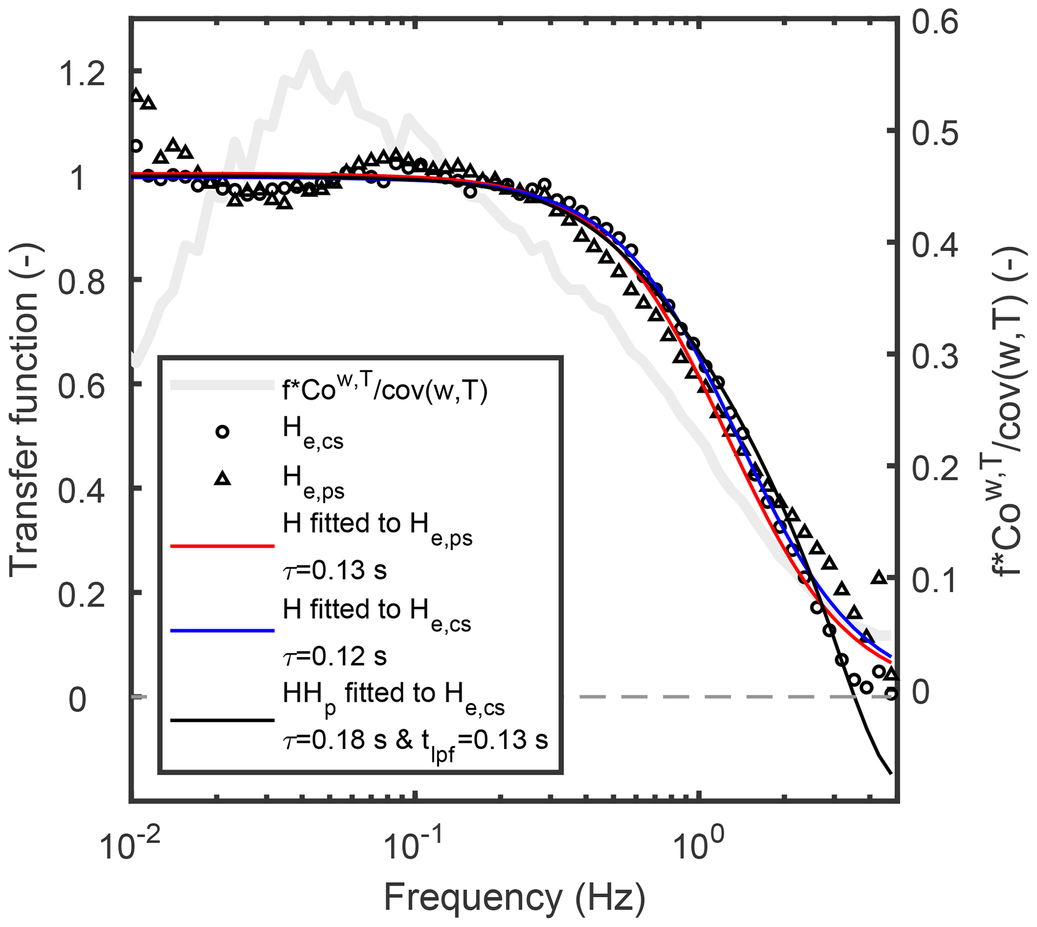
Figure 7 Empirical transfer functions estimated for CO₂ from ensemble-averaged cospectra (H_e,cs; Eq. 12) and power spectra (H_e,ps; Eq. 13) and three fits to the empirical transfer functions. Also the corresponding frequency-weighted normalised average cospectrum related to heat flux is shown (grey line) in order to illustrate the frequency range with the highest contribution to the scalar fluxes. Data from Siikaneva were used.

Based on theoretical considerations (Sect. 2) and results obtained with attenuated T time series, H fit to H_e,cs (Method 2) was projected to estimate smaller response times than the other two methods that were projected to agree (see, for example, Fig. 5b). Instead, here for CO₂ the HH_p fit to H_e,cs gave longer response times than the other two methods (Fig. 7). For signals with small attenuation both τ and t_lpf are likely difficult to estimate accurately by fitting HH_p to H_e,cs. The low-pass-filtering-induced lag (t_lpf) can attain values only with the temporal resolution of the data being processed (here 0.1 s), and hence for time series exhibiting small attenuation t_lpf may well be zero. This would cause H_e,ps and H_e,cs to be similar, and hence they would result in similar estimates for the response time, as observed here for CO₂. This granular estimation of t_lpf might explain why the response times for CO₂ did not follow the expectations. It should be also noted that the methods to estimate the response time have a limited accuracy of estimation stemming from the algorithms used in the estimation, instrument limitations and meteorological conditions under which the observations are made (Aslan et al., 2021). Furthermore, the empirical transfer function derived from cospectra (H_e,cs) contains the attenuation related also to sensor separation (Horst and Lenschow, 2009), whereas the empirical transfer function estimated from power spectra (H_e,ps) is related only to gas-analyser-induced low-pass filtering.

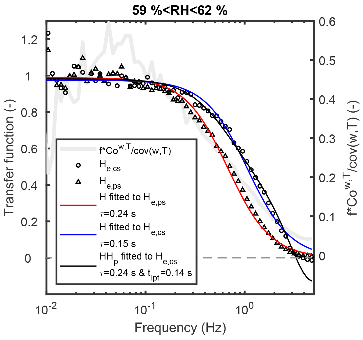
Figure 8 Similar figure as Fig. 7 but for H₂O in moderate relative humidity conditions (59 % < RH < 62 %). Note that τ estimated from H_e,ps agrees with τ estimated from H_e,cs with HH_p. Data from Siikaneva were used.

For H₂O, τ depends on RH (Mammarella et al., 2009; Ibrom et al., 2007a; Runkle et al., 2012), and hence the analysis was done in RH bins. Figure 8 shows an example of empirically derived transfer functions for H₂O at Siikaneva in moderate relative humidity conditions. H_e,cs showed less high-frequency attenuation than H_e,ps due to cross-covariance maximisation as predicted by the theory (Sect. 2). HH_p fit to H_e,cs resulted in a similar value for τ as the one obtained by fitting H to H_e,ps. The other fitting parameter in HH_p fit (t_lpf) was 0.14 s, indicating the low-pass filtering of H₂O time series caused an additional lag to the H₂O time series. Note that H does not perfectly describe the shape of H_e,ps. This is due to adsorption and desorption of H₂O to sampling tube walls, a process which cannot be described accurately with Eq. (3) (Nordbo et al., 2013). Hence different transfer functions have been proposed for H₂O (De Ligne et al., 2010; Nordbo et al., 2014).

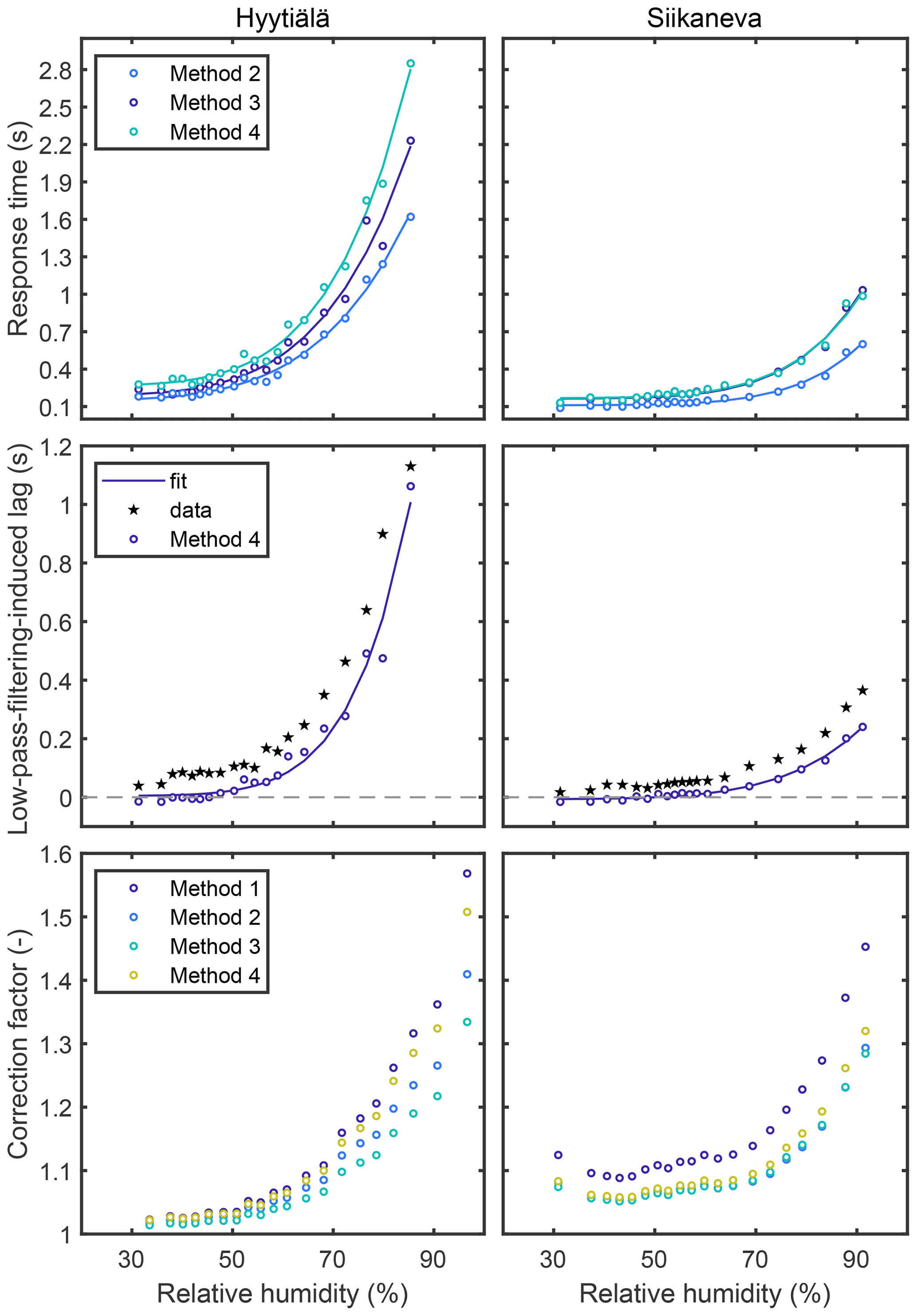
Figure 9 Response times (top row), low-pass-filtering-induced time lags (middle row) and correction factors (bottom row) as a function of relative humidity. Results for Hyytiälä pine forest are on the left and for Siikaneva open peatland on the right. The lines describe the fits used to obtain τ and t_lpf values for the CF calculation (see Sect. 3.2.1).

Figure 9 shows results obtained for H₂O in different RH bins at the two sites. The H fit to H_e,cs (Method 2) gave smaller values for τ in agreement with the results obtained with attenuated T (Fig. 5b) and expectations based on the theory (Sect. 2). The HH_p fit to H_e,cs (Method 4) was able to reproduce the H₂O time-lag dependency on RH, yet it estimated systematically smaller values for the time-lag difference between H₂O and CO₂ than those obtained with cross-covariance maximisation. The time-lag difference between H₂O and CO₂ can be assumed to be related to t_lpf of H₂O since H₂O is more attenuated than CO₂. The difference between H₂O and CO₂ time lags obtained with cross-covariance maximisation showed linear dependence on estimated response times in relative humidity bins with a similar dependency at both sites ($y=ax+b$, where a=0.47 and b = −0.05 s for Siikaneva and a=0.44 and b = −0.07 s for Hyytiälä, and where y is the time-lag difference and x the response time. Fits were based on orthogonal linear regression). Difference between H₂O and CO₂ time lags resulted from stronger low-pass filtering of H₂O than CO₂ signal, and this analysis assumes that the mere travel times through the sampling lines (i.e. t_phys), which do not depend on the low-pass filtering effects, were the same for H₂O and CO₂. These results are in line with Fig. 2 where it was shown that the low-pass-filtering-induced time lag was primarily determined by a linear dependence on τ with a secondary dependence on turbulence timescale. However, the slopes obtained above were different from the ones derived in Sect. 4.1.

The CF values estimated with the four methods agreed at Hyytiälä for low RH periods, but they diverged at high RH periods. For instance when RH > 80 % the four methods gave on average 1.39, 1.29, 1.23 and 1.37 at the Hyytiälä site, respectively. These results are in line with the ones obtained with attenuated T time series (Sect. 4.2 and Fig. 5a): when τ was large, Method 1 overestimated and Method 3 underestimated CF, similar as here for H₂O at high RH (and hence large τ). In contrast, for Siikaneva Method 1 gave systematically higher values for the correction factor regardless of RH, whereas the other three methods gave more similar CF RH dependency. This difference to Hyytiälä was likely due to lower τ values also at high RH (Fig. 9). Note also that the EC measurement set-up (measurement height, gas sampling system) was not identical at the two sites.

Table 3 Relative difference between the mean CO₂ and H₂O fluxes obtained with the different correction methods ($\left(\text{cor-ref}\right)/\text{ref}\cdot \mathrm{100}\mathit{\%}$). Fluxes corrected with Method 4 were used as a reference for the other three methods. All values are in per cent (%).

On average, the differences between the four different methods to calculate CF were small, typically within ± 3 % at both sites for both gases (CO₂ and H₂O) (Table 3). The biggest mean relative difference (4.1 %) was found for H₂O measurements at the Siikaneva site for Method 1. This was likely due to the combination of low measurement height and high attenuation which resulted in biased CF values, in accordance with the findings obtained with the attenuated T time series (Fig. 6a). Interestingly, for CO₂ the biggest difference at both sites was obtained with Method 3, yielding smaller fluxes than the reference (Method 4). The difference was bigger than the one obtained with Method 1 which contradicts the findings presented above with attenuated T (Sect. 4.2 and Table 2) and expectations based on theory (Sect. 2), although the differences found between the methods were generally small. Note that if t_lpf≈0, then both power spectra and cospectra are attenuated similarly (i.e. with H) resulting in methods 1, 2 and 4 being similar. Infrared gas analysers for CO₂ and H₂O can often be mounted close to the inlet, and in both set-ups considered here inlet lines are fairly short. The measurement of other gases, including CH₄ and N₂O, usually requires larger equipment which often has to be operated on the ground and/or some distance away from the mast, requiring longer inlet lines with slow time response. In these situations the correct shape of the cospectral transfer function matters a lot more than for the measurement set-ups included here, and hence the variability between methods is expected to be larger.

4.4 Correct form for cospectral transfer function

There has been a long-standing debate about what the correct form for cospectral transfer function is when the scalar measurements are done with a first-order linear sensor and vertical wind speed is not attenuated. The seminal paper on EC frequency-response corrections by Moore (1986) described the flux attenuation related to the scalar sensor with $\sqrt{H}$ (see Eq. 5), which was later deemed erroneous, for example, by Eugster and Senn (1995), Horst (1997, 2000), and others. Partly based on similar derivations as shown here in Sect. 2, the correct form for the cospectral transfer function was argued by Horst (1997, 2000) and Massman (2000) to be H instead of $\sqrt{H}$ . Lately, both forms (H and $\sqrt{H}$) have been utilised in the literature (e.g. Fratini et al., 2012; Foken et al., 2012b; Mammarella et al., 2016; Hunt et al., 2016; Wintjen et al., 2020) without clear consensus on which one is correct. Part of this confusion is likely related to the fact that some of the past studies have been using incorrect terminology by using the term cospectral transfer function (Eq. 5) even though they have derived/utilised a transfer function for the amplitude spectrum (Eq. 10).

Briefly summarising the findings in this study, it was shown in Sect. 2 in accordance with, for example, Horst (2000) that in the case the travel time in the gas sampling system could be accurately estimated and accounted for, the attenuation of cospectrum (and hence flux) could be described with H. However, cross-covariance maximisation inadvertently accounts also for the scalar low-pass-filtering-related time shift (t_lpf) and consequently induces a phase shift between the lag-corrected attenuated scalar and vertical wind time series. Hence in the case that cross-covariance maximisation is used to align the two time series, the correct form for cospectral transfer function is HH_p, in which the part related to the phase shift (H_p) is calculated with t_lpf. It was shown above that HH_p can be approximated with $\sqrt{H}$. Therefore the debate about which is the correct form for cospectral transfer function (H or $\sqrt{H}$) relates to the low-pass-filtering-induced phase shift as discussed already by Eugster and Senn (1995) and Horst (2000), albeit with a different conclusion. Note, however, that $\sqrt{H}$ is an approximation and not an exact representation of the cospectral transfer function.

5 Summary and conclusions

The influence of low-pass-filtering-induced phase shift on estimation of high-frequency response of an EC set-up was analysed. The analysis assumed that the EC set-up consisted of a fast-response anemometer and a linear, first-order-response scalar sensor. Spectral corrections aiming at correcting the EC fluxes for low-pass filtering were estimated with four methods: three widely used methods and one newly proposed method which specifically accounts for the interaction between the low-pass-filtering-induced phase shift and attenuation. Based on theoretical considerations and experimental results we come to the following conclusions:

• Cross-covariance maximisation overestimates the signal travel time in the EC sampling line since it inadvertently accounts also for the lag caused by low-pass filtering of scalar time series caused by the non-ideal measurement system. The bias in the estimated time lag depends linearly on low-pass-filter response time (τ) with a small additional dependence on turbulence timescale. Hence, other means for estimating the physical time lag might be warranted, especially in the case of noisy measurements (Langford et al., 2015). Further research on this topic is required.

• Both power spectra and cospectra are attenuated with the same transfer function (H, as noted also by Horst, 2000) in the case that the travel time of the scalar signal in the sampling line can be accurately estimated. However, if cross-covariance maximisation is used, then attenuation of cospectra follows HH_p in which H_p accounts for the bias in the estimated travel time caused by cross-covariance maximisation, and it was shown that HH_p can be roughly approximated with $\sqrt{H}$. Therefore, all flux calculation algorithms which rely on cross-covariance maximisation and at the same time use H to describe the attenuation of the cospectra (e.g. Horst, 1997; Massman, 2000) can be projected to be biased in the same way as Method 1 used here if the response time (i.e. τ) is accurately estimated (e.g. from power spectra). In these cases the bias in EC fluxes can be 10 % or above for short tower measurements with moderate attenuation. Hence, data reprocessing is warranted in order to rectify this bias.

• In order to estimate and correct for the flux attenuation correctly, it is vital to accurately describe the attenuation of the cospectra in the correction procedure. Hence, while fitting H to cospectra (Method 2) biased the first-order response time due to the use of the incorrect cospectral transfer function, it resulted only in a small bias for the flux correction factor since the method describes the attenuation of cospectra accurately once the cross-covariance maximisation has been applied. By contrast, fitting of H to power spectra (Method 1) correctly estimates the response time, but it nevertheless yields biased flux corrections since it utilised a transfer function that is incorrect when estimating the flux using cross-covariance maximisation.

• The theoretical framework proposed in this paper was able to describe the changes in H₂O time lag as H₂O response time increased with relative humidity. This suggests that the findings derived here with attenuated temperature time series are applicable also in real world situations for EC gas flux measurements. However, results for CO₂ deviated from the expectations based on the theory. Reasons for this remained unclear; however, low-pass filtering of inert gases (such as CO₂) in the gas sampling line may deviate from what was described here in such a way that the low-pass filter acting on CO₂ may not induce a phase shift. This should be investigated by using CO₂ flux data from an EC set-up with pronounced attenuation of CO₂ fluctuations in the sampling line or alternatively in a controlled environment in a laboratory (Metzger et al., 2016; Aubinet et al., 2016).

In summary, it is suggested that the spectral correction methods implemented in EC data processing software are revised so that the influence of low-pass-filtering-induced phase shift is recognised following the findings presented above. In particular, the usage of Method 1 is discouraged as it resulted in clearly biased flux values.

Appendix A: Derivation of Eq. (4)

Here we derive Eq. (4) starting from the cross-spectrum (Eq. 2):

$$\begin{array}{}\text{(A1)}& {\text{Cr}}_{\mathrm{m}}=\left[Z_{\mathrm{w}}\right]{\left[h_{\mathit{\chi }}{Z}_{\mathit{\chi }}\right]}^{*}{e}^{-j{\mathit{\varphi }}_{\text{phys}}},\end{array}$$

where h_χ can be described with Eq. (3), which gives

$$\begin{array}{}\text{(A2)}& {\displaystyle }{\text{Cr}}_{\mathrm{m}}& {\displaystyle }=\left[Z_{\mathrm{w}}\right]{\left[{\displaystyle \frac{Z_{\mathit{\chi }}}{\mathrm{1}-j\mathit{\omega }\mathit{\tau }}}\right]}^{*}{e}^{-j{\mathit{\varphi }}_{\text{phys}}},\text{(A3)}& {\displaystyle }{\text{Cr}}_{\mathrm{m}}& {\displaystyle }=\left[Z_{\mathrm{w}}\right]\left[{\displaystyle \frac{Z_{\mathit{\chi }}^{*}}{\mathrm{1}+j\mathit{\omega }\mathit{\tau }}}\right]e^{-j{\mathit{\varphi }}_{\text{phys}}},\text{(A4)}& {\displaystyle }{\text{Cr}}_{\mathrm{m}}& {\displaystyle }=Z_{\mathrm{w}}{Z}_{\mathit{\chi }}^{*}{\displaystyle \frac{\mathrm{1}}{\mathrm{1}+j\mathit{\omega }\mathit{\tau }}}{e}^{-j{\mathit{\varphi }}_{\text{phys}}},\text{(A5)}& {\displaystyle }{\text{Cr}}_{\mathrm{m}}& {\displaystyle }={\displaystyle \frac{\text{Co}+jQ}{\mathrm{1}+j\mathit{\omega }\mathit{\tau }}}{e}^{-j{\mathit{\varphi }}_{\text{phys}}},\text{(A6)}& {\displaystyle }{\text{Cr}}_{\mathrm{m}}& {\displaystyle }={\displaystyle \frac{(\text{Co}+jQ)(\mathrm{1}-j\mathit{\omega }\mathit{\tau })}{\mathrm{1}+{\mathit{\omega }}^{\mathrm{2}}{\mathit{\tau }}^{\mathrm{2}}}}{e}^{-j{\mathit{\varphi }}_{\text{phys}}},\text{(A7)}& {\displaystyle }{\text{Cr}}_{\mathrm{m}}& {\displaystyle }={\displaystyle \frac{(\text{Co}-j\mathit{\omega }\mathit{\tau }\text{Co}+jQ+\mathit{\omega }\mathit{\tau }Q)}{\mathrm{1}+{\mathit{\omega }}^{\mathrm{2}}{\mathit{\tau }}^{\mathrm{2}}}}{e}^{-j{\mathit{\varphi }}_{\text{phys}}},\end{array}$$

where $Z_{\mathrm{w}}{Z}_{\mathit{\chi }}^{*}=\text{Co}+jQ$ was utilised. Next the quadrature spectrum (Q) was assumed to be zero (Horst, 1997; Massman, 2000) and hence

$$\begin{array}{}\text{(A8)}& {\text{Cr}}_{\mathrm{m}}={\displaystyle \frac{\text{Co}-j\mathit{\omega }\mathit{\tau }\text{Co}}{\mathrm{1}+{\mathit{\omega }}^{\mathrm{2}}{\mathit{\tau }}^{\mathrm{2}}}}{e}^{-j{\mathit{\varphi }}_{\text{phys}}}.\end{array}$$

Now we can use Euler formula ($e^{-j{\mathit{\varphi }}_{\text{phys}}}=\cos {\mathit{\varphi }}_{\text{phys}}-j\sin {\mathit{\varphi }}_{\text{phys}}$):

$$\begin{array}{}\text{(A9)}& {\displaystyle }{\text{Cr}}_{\mathrm{m}}={\displaystyle \frac{\text{Co}-j\mathit{\omega }\mathit{\tau }\text{Co}}{\mathrm{1}+{\mathit{\omega }}^{\mathrm{2}}{\mathit{\tau }}^{\mathrm{2}}}}(\cos {\mathit{\varphi }}_{\text{phys}}-j\sin {\mathit{\varphi }}_{\text{phys}}),\text{(A10)}& {\displaystyle }{\text{Cr}}_{\mathrm{m}}={\displaystyle \frac{\left[\begin{array}{c}\text{Co}\cos {\mathit{\varphi }}_{\text{phys}}-j\mathit{\omega }\mathit{\tau }\text{Co}\cos {\mathit{\varphi }}_{\text{phys}}\\ -j\text{Co}\sin {\mathit{\varphi }}_{\text{phys}}-\mathit{\omega }\mathit{\tau }\text{Co}\sin {\mathit{\varphi }}_{\text{phys}}\end{array}\right]}{\mathrm{1}+{\mathit{\omega }}^{\mathrm{2}}{\mathit{\tau }}^{\mathrm{2}}}},\text{(A11)}& {\displaystyle }\begin{array}{rl}{\text{Cr}}_{\mathrm{m}}=& {\displaystyle \frac{\cos {\mathit{\varphi }}_{\text{phys}}-\mathit{\omega }\mathit{\tau }\sin {\mathit{\varphi }}_{\text{phys}}}{\mathrm{1}+{\mathit{\omega }}^{\mathrm{2}}{\mathit{\tau }}^{\mathrm{2}}}}\text{Co}\\ & -j{\displaystyle \frac{\sin {\mathit{\varphi }}_{\text{phys}}\mathit{\omega }\mathit{\tau }\cos {\mathit{\varphi }}_{\text{phys}}}{\mathrm{1}+{\mathit{\omega }}^{\mathrm{2}}{\mathit{\tau }}^{\mathrm{2}}}}\text{Co},\end{array}\end{array}$$

which equals Eq. (4) in Sect. 2.