A powerful lidar system capable of 1 h measurements of water vapour in the troposphere and the lower stratosphere as well as the temperature in the upper stratosphere and mesosphere

A high-power Raman lidar system has been installed at the high-altitude research station Schneefernerhaus (Garmisch-Partenkirchen, Germany) at 2675 $\mathrm{m}\mathrm{a}.\mathrm{s}.\mathrm{l}.$, at the side of an existing wide-range differential absorption lidar (DIAL). An industrial XeCl laser was modified for linearly polarized single-line operation at an average power of about 180 W. This high power and a 1.5 m diameter receiver allow us to extend the operating range for water-vapour sounding to 20 km for a measurement time of just 1 h, at an uncertainty level of the mixing ratio of 1 to 2 ppm. This was achieved for a vertical resolution varied between just 0.2 and 0.6 km in the stratosphere. The lidar was successfully validated with a balloon-borne cryogenic frost-point hygrometer (CFH). In addition, temperature measurements up to altitudes of around 87 km were demonstrated for 1 h of signal averaging. The system has been calibrated with the DIAL, the CFH and radiosondes.

1 Introduction

Water vapour in the upper troposphere and lower stratosphere (UTLS) is the key factor controlling how much thermal infrared radiation escapes from the atmosphere into space (e.g. Kiehl and Trenberth, 1997; Schmidt et al., 2010; Lacis et al., 2013). In a warmer climate, the atmosphere takes up more water vapour from the sea surface. However, this increase could be counteracted by additional cloud formation and precipitation. Also vertical exchange processes could change in a warmer climate (Trickl et al., 2010a, 2020a). Water-vapour trends in the troposphere derived from observations are discussed in literature. Paltridge et al. (2009) report negative trends for the period 1973 to 2007 at all free tropospheric altitudes in NCEP (National Centers for Environmental Prediction; https://www.ncep.noaa.gov/, last access: 20 January 2021) reanalysis data, in particular in the upper troposphere, in contrast to the expectations from climate modelling. Other studies show at least regionally positive trends (Ross and Elliott, 2001; Mieruch et al. 2008; Chen and Liu, 2016). However, they evaluate columnar quantities that are dominated by the moist boundary layer, where thermal radiation is trapped by water vapour anyway. In the lower stratosphere, the Boulder series shows a trend reversal from positive to negative that occurred around 2000 (Hurst et al., 2011), but the pronounced positive trend during the early phase since the late 1980s is not confirmed for other locations (Solomon et al., 2010; Hegglin et al., 2014).

Due to the role of water vapour as the most important greenhouse gas, the optimization of high-accuracy, range-resolved vertical sounding instrumentation covering the entire free troposphere and the lower stratosphere has become more and more important during the past 2 decades (Kämpfer et al., 2013). All the most commonly used sensors used for routine measurements have limitations. Operational radiosondes have been greatly improved within the troposphere in recent years, but deficiencies exist in the very cold tropopause region and the lower stratosphere, where the sensors exhibit slow response and low sensitivity (Miloshevich et al., 2006; Vömel et al., 2007a; Steinbrecht et al., 2008; Kämpfer et al., 2013). Balloon-borne cryogenic frost-point hygrometers (CFHs; Vömel et al., 2007b, 2016; Kämpfer et al., 2013; Hurst et al., 2016) and Lyman-α hygrometers (Kley and Stone, 1978; Weinstock et al., 1990; Khattatov et al., 1994; Hintsa et al., 1999; Zöger et al., 1999; Kämpfer et al., 2013), though being highly accurate, are rarely used in dense routine measurement programmes due to their elevated costs. Ground-based microwave radiometers have an excellent temporal coverage, but their application is limited to the lower and middle troposphere (Westwater, 1978; Han and Westwater, 1995; Solheim and Godwin, 1998) and altitudes above 20 km (Nedoluha et al., 1997; Deuber et al., 2004, 2005; Kämpfer et al., 2013), with somewhat limited vertical resolution. The value of satellite-borne measurements (Kämpfer et al., 2013) is limited by the considerable spatial averaging that results in a loss of information due to the high variability of water vapour, even in the lower stratosphere (Zahn et al. 2014), but can yield reasonable averages and global coverage (e.g. Solomon et al., 2010).

There is just one long quantitative ground-based sounding series of stratospheric water vapour, obtained with the Boulder balloon-borne CFH (Scherer et al., 2008; Hurst et al., 2011). These measurements have been carried out since 1980 at intervals of about one measurement per month. Because of the considerable variability of water vapour up to at least the UTLS, more frequent measurements with good vertical resolution are desirable (Müller et al., 2016). This variability is caused to a major extent by transport-induced patterns. Injections of water vapour into the stratosphere occur not only in the tropics (Rosenlof, 2003), where freeze-drying has also been claimed to matter (see, for example, the discussions by Peter et al., 2003, Luo et al., 2003, Jensen et al., 2007, and Zahn et al., 2014), but also in the jet-stream regions (Stohl et al., 2003; and references therein). Warm conveyor belts (WCBs) can lift moist polluted air from the boundary layer to the tropopause region (Stohl and Trickl, 1999). Overshooting WCBs even transfer water vapour into the lower stratosphere (LS; Stohl, 2001), although possibly diminished by dehydration due to cirrus–cloud formation (cirrus clouds being almost ubiquitous in WCB air probed by our lidar systems). Most investigations related to this topic have been limited to airborne measurements of the chemical composition of the tropopause region (e.g. Pan et al., 2007; Gettelman et al., 2011; Zahn et al., 2014). It is reasonable to assume that water vapour transported into the LS by troposphere–stratosphere transport (TST) is an important target for vertical sounding of H₂O with enhanced temporal density. The opposite mechanism, stratosphere–troposphere transport (STT), is much more important than previously thought, at least in central Europe after an increase over several decades (Trickl et al., 2010a; 2020a). Growing STT can contribute to a lowering of the tropospheric humidity.

Lidar-based measurements have the potential of good temporal and vertical resolution and are, therefore, attractive for resolving transport-related concentration changes. However, the use of lidar systems for water vapour implies a major challenge due to the strong decrease of both the backscatter signal and the water-vapour concentration with altitude. Despite the problems related to the extreme signal dynamics, the NDACC (Network for the Detection of Atmospheric Composition Change) Lidar Working Group has strongly advocated developing powerful ground-based water-vapour lidar systems with UTLS capability, with a focus on the Raman lidar technique. Several Raman lidar systems have already reached a reasonable UTLS performance (Congeduti et al., 1999; Whiteman et al., 2010; Dionisi et al., 2012, 2015; Leblanc et al., 2012; Vérèmes et al., 2019). Whiteman et al. (2010), Leblanc et al. (2012) and Vérèmes et al. (2019) demonstrated vertical ranges extending to more than 20 $\mathrm{km}\mathrm{a}.\mathrm{s}.\mathrm{l}.$ for averaging over many hours.

The most important detection barrier in the lower stratosphere is the very small mixing ratio of water vapour of 4 to 5 ppm (e.g. Hurst et al., 2011). In principle, this would require a highly sensitive approach. Measurements of molecules in a range far below 1 ppt with respect to normal conditions can be achieved in the laboratory, even under restrictive conditions (e.g. Trickl and Wanner, 1983; Trickl et al., 2010b). However, a fluorescence lidar approach cannot be used for atmospheric H₂O because it electronically absorbs in the vacuum ultraviolet spectral region and undergoes photodissociation as concluded from the diffuse bands (e.g. Yoshino et al., 1997). As a consequence, lidar measurements of H₂O in the lower atmosphere are restricted to the differential absorption lidar (DIAL) and Raman scattering methods. The detection sensitivity and the range of the DIAL method are limited by the signal noise of the absorption measurement. Raman scattering is the least sensitive approach. However, night-time Raman scattering is a so-called background-free method. Thus, the sensitivity to water vapour can, in principle, be driven to any level by enhancement of the laser power and the diameter of the receiver, as long as allowed by financial or technical restrictions. Very importantly, a Raman lidar can be operated at wavelengths for which absorption in the atmosphere is negligible.

For a Raman lidar calibration with an external source, there is an important issue: the optical transmission data of a Raman lidar and the Raman scattering cross sections cannot be determined with sufficient accuracy. In addition, a degradation of the components must be taken into consideration. Thus, a trace-gas Raman lidar routinely operated over an extended period of time must be repeatedly calibrated with external references, and the stability of the calibration must be verified. Mostly, radiosonde measurements are used as reference (e.g. Leblanc and McDermid, 2008; Dionisi et al., 2010), but also calibration with H₂O column measurements are reported (Barnes et al., 2008; Vérèmes et al., 2019). However, the Raman lidar systems are not necessarily located at routine balloon sounding stations. Even for on-site sonde launches, the sondes usually rapidly drift away from the lidar, which frequently results in discrepancies due to the high spatial variability of water vapour (Vogelmann et al., 2011, 2015). Infrequent comparisons with sondes necessitate additional performance control such as built-in lamps (Dionisi et al., 2010; Leblanc and McDermid, 2008, 2011; Leblanc et al., 2012; Whiteman et al., 2011) or monitoring of the radiation backscattered from air or nitrogen.

At Garmisch-Partenkirchen, we first concentrated on the differential absorption lidar (DIAL) technique for measuring free tropospheric water vapour (Vogelmann and Trickl, 2008; Trickl et al., 2013, 2014, 2015, 2016, 2020a). This system has the great advantage of a good daytime performance. In recent years, a high-power Raman lidar has been built that extends the range of the DIAL into the lower stratosphere during night-time with a data-acquisition time of just 1 h. Both systems are operated side by side at the Schneefernerhaus mountain station (UFS, Umweltforschungsstation Schneefernerhaus; 47^∘25^′00^′′ N, 10^∘58^′46^′′ E) at an altitude of 2675 m, which offers the possibility of direct and accurate calibration of the Raman lidar. The DIAL has been thoroughly validated and is free of bias at an uncertainty level of 1 % of average concentrations or less (Vogelmann, et al., 2011; Trickl et al., 2016). Both systems probe the same atmospheric volume and can be very reliably compared up to about 8 km where the DIAL data start to become noisy.

The large system allows us to make temperature measurements up to the mesosphere based on an established approach for inverting the Rayleigh backscatter signal for 355 nm (Hauchecorne and Chanin, 1980). In this way, not only the primary greenhouse gas, but also the most important climate parameter is provided.

In this paper we report the development and the current state of the Raman lidar, before the begin of routine measurements. We describe the steps to achieve up to 180 W of linearly polarized and single-line output from a modified industrial xenon-chloride laser (308 nm) (Sect. 3) and the development of the far-field receiver featuring a primary mirror with a diameter of 1.5 m (Sect. 4). Parallel to the ozone DIAL at IMK-IFU (Trickl et al., 2020b), a significant step forward in signal processing was made. The highly satisfactory lidar performance is demonstrated by examples of 1 h atmospheric measurements, also including a first demonstration of a temperature measurement up to 87 km (Sects. 6 and 7). Finally, conclusions and suggestions for upgrading the lidar are made (Sect. 8).

2 Simulation of the system performance

Before finalizing the first version of the lidar design a number of simulations of the system performance were made. Figure 1 shows the results. We assumed 200 W of laser power at 308 nm (as suggested by the laser specifications available at that time), a receiver diameter of 1.5 m, a range bin of 200 m, 10 % detection efficiency and a measurement time of 1 h. The atmospheric data were taken from the mid-latitude summer model of the LOWTRAN simulation program (Kneizys et al., 1988).

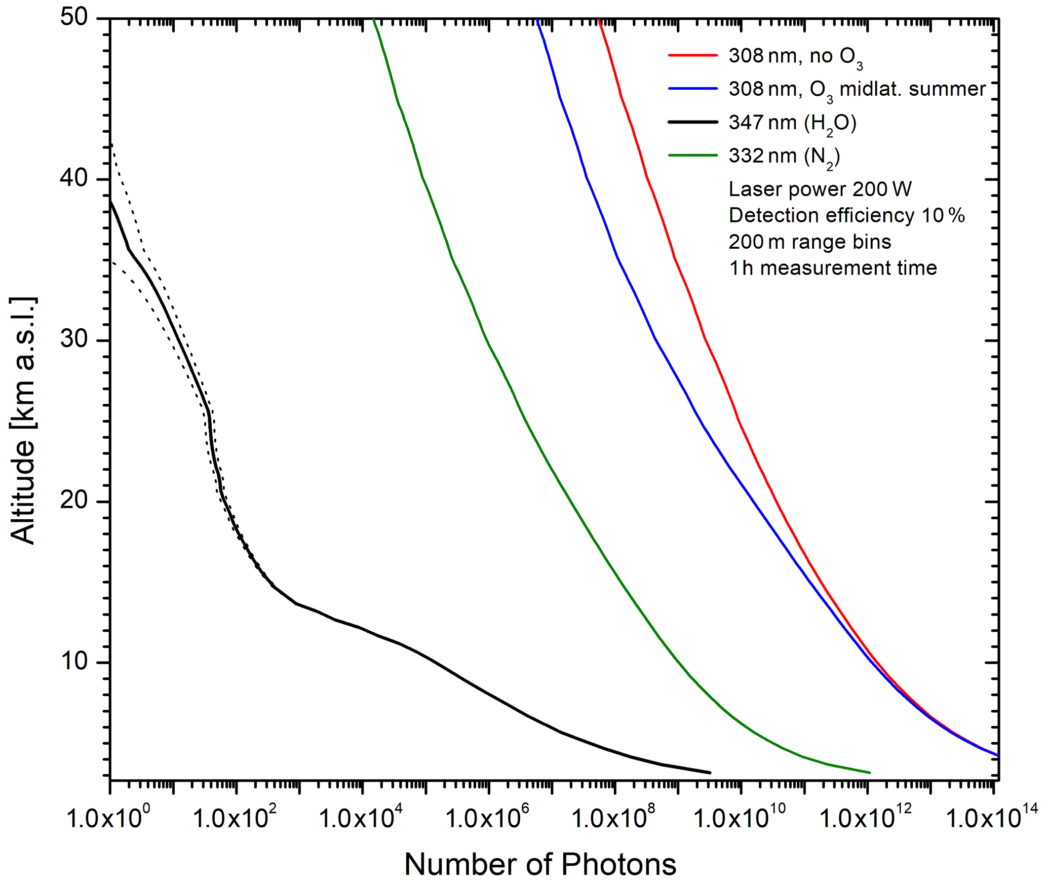
Figure 1 Simulations of the backscatter signals for four wavelengths specified in the upper right corner; an average laser power at 308 nm of 200 W, a receiver diameter of 1.5 m, a detection efficiency of 10 %, a range bin of 200 m and a measurement time of 1 h were assumed.

The simulation revealed that the Raman backscatter signal for stratospheric water vapour is roughly 8 orders of magnitude smaller than the Rayleigh backscatter signal for 308 nm. This imposes extreme boundary conditions for the optical system (Sect. 3.3). The effect of the signal loss at 308 nm due to the absorption by ozone is not very severe up to 20 km. In comparison with the most commonly used primary wavelength of 355 nm, this loss is roughly compensated for by the fourth-order frequency dependence of the Raman backscatter coefficient.

The atmospheric measurements demonstrate that the simulation is realistic (Sect. 8).

Table 1 Transmitter details.

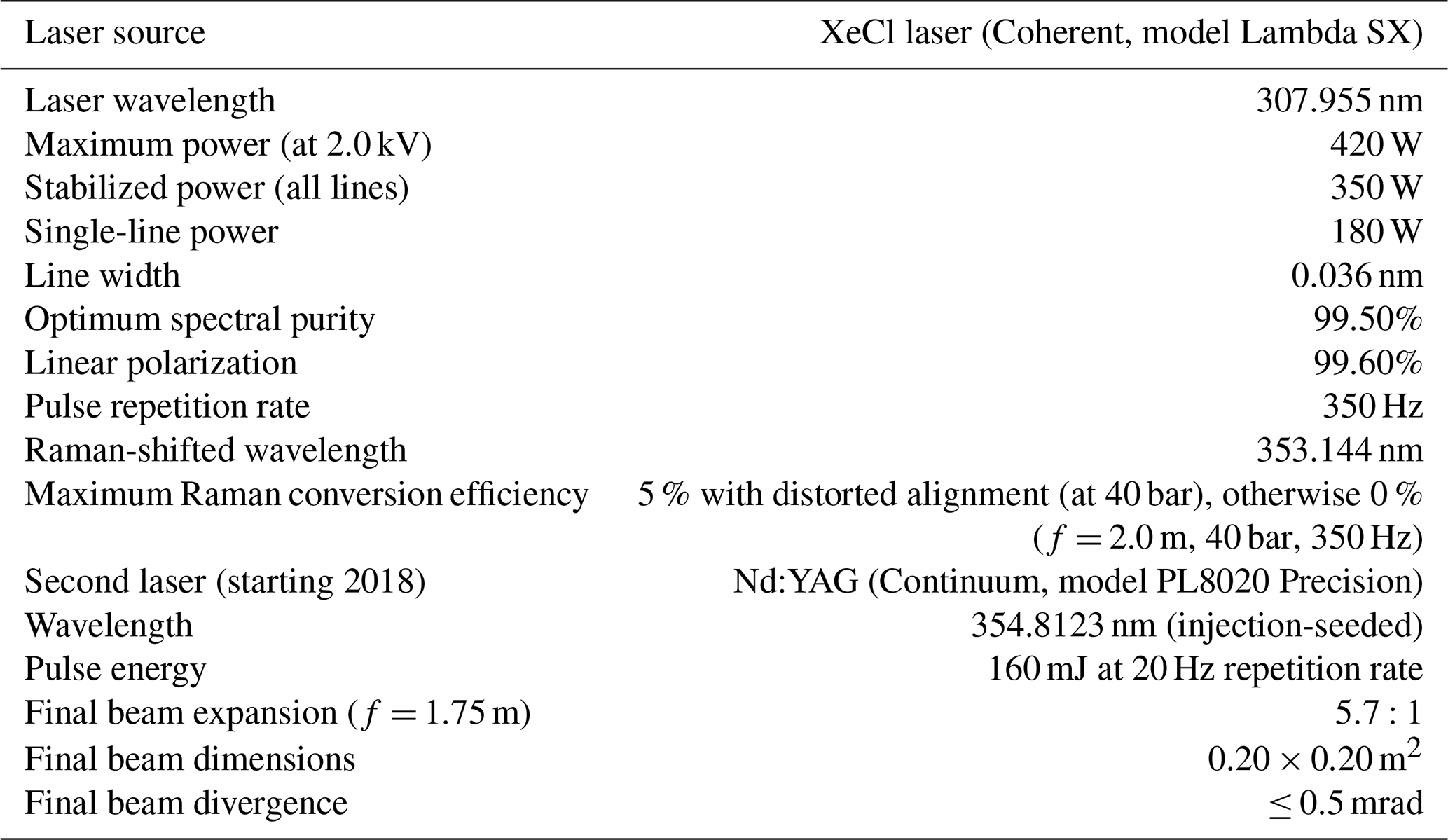
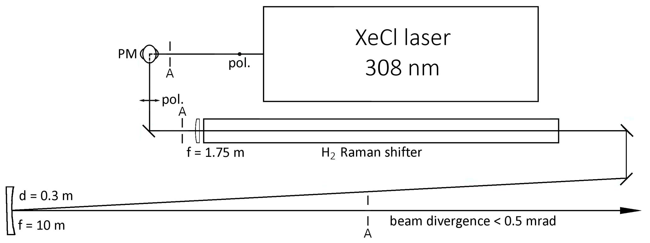
Figure 2 Overview of the transmitter part of the UFS Raman lidar: the laser beam profile is expanded to a 36 × 36 mm² square shape by a f = −100 mm–f = 250 mm pair of cylindrical lenses (recently removed), sent down by a combination of two plane mirrors (rotating the polarization by 90^∘) before it is focussed into a vacuum cell (originally Raman shifter), 3.6 m long with a f = 1.75 m lens (initially f = 2.0 m). The beam diverges from the focal point, is collimated by an f = 10 m concave mirror and reaches the motorized beam-steering mirror in a vertical exit shaft outside the laboratory (not shown). Three apertures allow us to control the beam pointing.

3 Laser system

3.1 General description

Figure 2 gives an overview of the transmitter section of the new UFS Raman lidar system in the rear part of the lidar laboratory (see also Table 1). The transmitter consists of a high-power laser, a hydrogen Raman shifter and a motorized (Astro System Austria, ASA) beam-steering mirror (not shown). The 0.5 m diameter beam-steering mirror sending the radiation into the atmosphere is located in a vertical emergency exit shaft outside the laboratory. All dielectrically coated optics, in particular the large-diameter mirrors, were supplied by Laseroptik G.m.b.H., unless explicitly stated differently.

The efficiency of Raman scattering scales as λ⁻⁴ and, thus, is the highest in the ultraviolet (UV) spectral region. Here, by far the most powerful radiation sources are excimer lasers. The radiation source used in our system is a big XeCl laser system with a power of 350 W (pulse energy 1 J, repetition rate 350 Hz, pulse length 80 ns) in energy-stabilized mode of operation that is normally used for industrial applications (Coherent Göttingen (formerly Lambda Physik), model Lambda SX 350C, size (l × w × h) = 2.500 m × 0.850 m × 1.925 m). The very high power of this laser system is much more important than the single-pass absorption loss in stratospheric ozone at the operating wavelength of 308 nm (Sect. 2). An ozone correction can be provided by a DIAL approach with an “off” emission at 353 nm (stimulated Raman shifting the laser radiation in H₂) or at 355 nm (frequency-tripled Nd:YAG laser).

The laser was transported to UFS by a cogwheel train of Zugspitzbahn A.G. There, it was lifted to the seventh floor of the building with the large elevator of UFS and then to the eighth floor with two pulleys, after removing the stairs.

Figure 3 Emission spectrum of a Coherent high-power XeCl laser in broadband operation (source: Coherent); the dashed red curve is the sum of three Gaussian lines with centres at 308.955, 308.173 and 308.215 nm and a full width at half maximum of 0.0357 nm.

As a consequence of its primarily industrial application, the laser system is operated under computer control, providing energy stabilization and numerous safety features. This is highly helpful for the planned automatic operation of the lidar system. However, a high beam divergence of nominally 1 mrad and 4 mrad in two perpendicular transverse orientations, random polarization and a three-line spectrum as shown in Fig. 3 are insufficient for the requirements of the lidar. Therefore, an approach had to be found for overcoming these disadvantages, considering the dangerous power level of this laser.

For our lidar concept, a linearly polarized narrowband radiation is needed. Injection seeding with a XeCl master oscillator with these properties was the premier choice because this could have resulted in maintaining high average power. However, this idea was given up because the manufacturer pointed out that there was no easy way of synchronization because of the specified 25 µs pulse-to-pulse jitter of the big laser and because of the considerable additional complexity and costs.

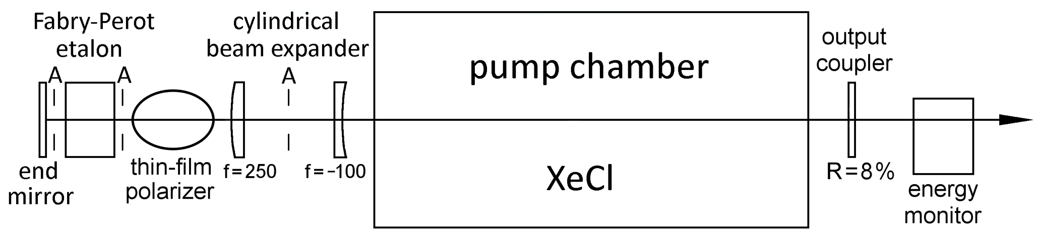
Figure 4 Top view of the modified Lambda SX laser system; 36 mm × 36 mm square apertures (A) are used for protecting optical components from potential powerful reflections from accidentally rotated components. The polarizer is oriented out of plane at Brewster's angle.

Instead, an intra-cavity solution was chosen. The resonator was stretched as shown in Fig. 4. The intra-cavity laser beam is first converted to an approximate squared cross section with another 2.5:1 cylindrical telescope in order to reduce the intensity in the new rear section. It is then fed through a Brewster-angle thin-film polarizer (transmittance 96 %) and a custom-made 70 mm diameter Fabry–Pérot etalon with 0.10 mm plate distance (SLS Optics Ltd.; R = 54 %, T_min ≈ 7 %, T_max = 95.4 %) to reach the 75 mm diameter end mirror. The large diameter of the etalon is expected to provide strong reduction of ablation of material by scattered UV radiation and the resulting ageing of the etalon plates. The chosen plate distance sets the free spectral range exactly to twice the wavelength difference between the two groups of emission lines in Fig. 3. When setting the transmission maximum to the short-wavelength component (307.955 nm; all wavelengths in this paper are specified for vacuum), the gain at the wavelength pair around 308.2 nm is suppressed, despite the residual transmittance of about 7 %. Just the direct first-pass forward emission estimated by the manufacturer to about 7 mJ cannot be avoided.

The beam divergence with our long cavity was smaller than that determined by the manufacturer. We measured a burning spot of 2.0 mm × 1.2 mm generated on a metal plate by focussing with a f = 2.0 m lens in front of the Raman shifter, corresponding to a divergence of 1.0 mrad × 0.6 mrad (most likely smaller than the full width of the intensity distribution). After the 5:1 beam expansion, the beam divergence is 0.2 mrad or less, an important prerequisite for ensuring a moderate size of the focal areas in the very large receiver and its polychromator.

3.2 Laser testing

3.2.1 General remarks

Despite the pronounced intra-cavity losses after multiple passes through the laser cavity, the maximum pulse energy achieved at repetition rates below 100 Hz is about 0.75 J. We explain this by fresh gain generated all along the 80 ns of laser emission and by 92 % of the amplified energy being emitted after each round trip. Thus, the losses do not matter similarly as in a cavity with higher reflectance of the output mirror.

3.2.2 Emission spectrum

For the laser operation we just slightly tilted the etalon vertically in order to avoid specular reflection. The wavelength is changed by horizontally tuning the etalon that is mounted on a motorized rotation stage (OWIS).

For monitoring the emission spectrum an inexpensive computer-controlled miniature grating spectrograph is used (Ocean Optics, HR 4000; Δλ = 0.07 nm). The performance of this spectrograph is highly satisfactory and stable as determined from a comparison of the 308.955 nm emission that is reproducibly obtained for maximum laser emission. Both the emissions around 308 and 353 nm are within the limited measurement range.

Figure 5 Spectrum of the laser emission with an almost optimized etalon angle; the laser was operated at a 10 Hz repetition rate, 1.75 kV load voltage and 663 mJ (including the polarizer).

In Fig. 5 we show a typical spectrum of the laser radiation obtained with the HR 4000 spectrograph. The etalon was rotated to concentrate the pulse energy almost exclusively in the low-wavelength spectral component. The etalon angle was not fully optimized to show the small impurity peak at 308.4 nm that is located at twice the distance between the strong line groups in Fig. 3 and, thus, most likely corresponds to another, weaker line of XeCl. Under optimum conditions, the impurity stays in the range between 1.0 % and 1.5 %. Further suppression would require an etalon with a slightly larger free spectral range.

The contribution of the longer wavelength doublet (308.2 nm) for an optimum etalon angle is less than 0.5 %. This value is in reasonable agreement with the 7 mJ of initial forward emission (Sect. 3.1), considering that just one-half of this weak broadband emission goes into the correct wavelength component (Fig. 3).

Given the specified 0.07 nm resolution of the HR 4000 spectrograph, the laser bandwidth is approximately 0.03 nm, in good agreement with the 0.0357 nm in the spectrum measured by Coherent in a high grating order (Fig. 3).

It is interesting to note that with an initially pronounced vertical tilt of the etalon, we achieved continuous single-line tuning of the laser, however with changing output pulse energy as a function of the horizontal tilt angle.

3.2.3 Polarizer

Linear polarization is mandatory for single-line stimulated Raman shifting (Kempfer et al., 1994) and for the wavelength-separation strategy in our receivers (Sect. 3.2). Therefore, a thin-film polarizer was mounted in the extended laser cavity, in the expanded section of the beam where the intensity is reduced. Despite the widened, quadratic beam profile, the substrate and the holder get rather warm after long operation of the laser at full power. This is caused by the absorption losses due to a maximum transmittance of just 94 %. Nevertheless, the degree of polarization of the laser output is as high as 99.4 %, in agreement with the expected 3.5 mJ (Sect. 3.1) of forward emitted radiation with wrong polarization after the first passage though the laser medium.

Laseroptik meanwhile promised the capability of producing thin-film polarizers with more than 99 % transmittance (as demonstrated for the polychromator). This would significantly reduce the thermal load and the intra-cavity radiation losses.

3.2.4 Alignment drifts

A careful warm-up procedure was seen as mandatory because of the long resonator. Any small thermally induced misalignment leads to a pronounced rotation of the laser beam inside and outside the cavity, which can lead to damage of components. Horizontal misalignment of the cavity starts to progress with a growing repetition rate that requires both the etalon and the end mirror being rotated horizontally. If the optical surfaces of the etalon stay perfectly parallel, the latter is difficult to understand and is tentatively ascribed to a combination of a slight mutual distortion of the etalon plates and the cylindrical telescope. Vertical corrections are mostly negligible.

Warm-up has been performed in 50 Hz steps. For each step, the etalon and the end mirror are realigned for maximum power after about 5 min of thermal equilibration. Very importantly, maximum power corresponds to optimum beam pointing and optimum spectral purity, which is highly welcome in view of automatic control of the modified laser. In the end, a highly stable operation of the laser is achieved over many hours, rarely requiring intervention.

For safety, six sand-blasted aluminium apertures were added as shown in Figs. 2 and 4, the first five of them with a cross section of 43 mm × 43 mm and the last one in the expanded beam; width × height = 200 mm × 120 mm. As mentioned, inside the laser cavity, even weak reflections can lead to damage at a maximum repetition rate. Outside the laser head, the apertures also help to control the beam pointing. At full power, metal plates must be used to localize the beam instead of paper sheets.

3.2.5 Laser pulse energy

In Fig. 6 the dependences of the pulse energy on the repetition rate and the load voltage, measured with the modified system, are shown. For each measurement, both the end mirror and the etalon were optimized.

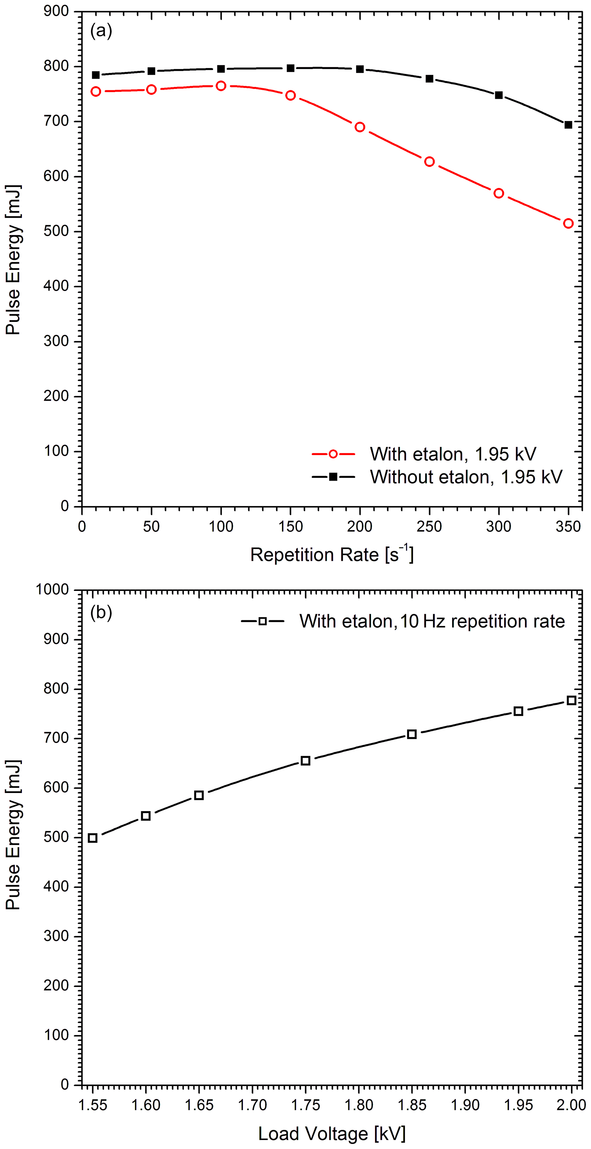
Figure 6 Optimized pulse energy as a function of the repetition rate (a) and the load voltage (b) for comparison. The maximum pulse energy of the broadband laser as delivered is 1.25 J (at 2.0 kV and 300 Hz).

The maximum pulse energy for a load voltage of 1.95 kV was 797 mJ without the etalon and 765 mJ with the etalon installed. This is much less than the 1.24 J at 1.95 kV and 300 Hz repetition rate achieved with the laser at the factory. Of course, there are considerable intra-cavity losses. These losses are mostly caused by the polarizer and the etalon but perhaps also by deficiencies in imaging in the cylindrical telescope or by achieving fewer round trips within the elevated-gain period due to the longer cavity. However, the overall losses are considerably stronger than the optical losses, as we estimate from the moderate reduction in pulse energy when inserting the etalon. We conclude that the most important drop in power is caused by the reduced number of round trips in the extended cavity.

With a growing repetition rate, the energy first increases, but above 150 Hz, it starts to drop considerably. This behaviour is not similarly pronounced without the etalon, as shown for comparison. It is, thus, ascribed to thermal stress in the etalon. The optimum pulse energy at 350 Hz achieved for clean optics was 515 mJ, resulting in a power of 180 W, 1 order of magnitude higher than in 355 nm Nd:YAG-based water-vapour Raman lidar systems in the past. The power slowly decreases further during a long night-time measurement period, most likely due to growing thermal issues. Under typical conditions we have operated the lidar in the range of 400 to 450 mJ, with aged gas even less. The pulse repetition rate was set to 300 Hz because of a time limitation in the data-acquisition system for operation with 16 000 bins.

The pulse energy at low repetition rates rises from 499 mJ at 1.55 kV to 777 mJ at 2.0 kV (Fig. 6b).

3.3 Raman shifter and beam expander

As routinely done in stratospheric ozone DIAL systems, we first applied stimulated Raman shifting in high-pressure hydrogen for generating an off wavelength of 353.144 nm (Klanner et al., 2012; Höveler et al., 2016) as a base for ozone corrections and a high-altitude temperature Rayleigh detection channel. We assumed that a conversion efficiency of a few per cent is sufficient for these purposes. In this way we could fulfil two goals, to minimize the loss of pulse energy in the fundamental wavelength for maximizing the detection sensitivity for water vapour and to reduce the uncertainty in the pulse-energy level at 308 nm needed for calibration of the H₂O Raman detection channel.

The 353 nm energy conversion efficiency was 19 % (f = 2.0 m) and more (f = 1.75 m) at a repetition rate of 10 Hz but did not exceed 3 % at a repetition rate of 350 Hz. This required very critical astigmatic focussing influenced by a cylindrical beam expander in front of the laser (no longer used, therefore missing in Fig. 2). With a well-collimated laser beam, no conversion was achieved at all at repletion rates beyond 100 Hz.

A new approach was introduced that is described below. The Raman shifter was then used just as a vacuum cell for the beam expander to avoid the optical breakdown in air.

3.4 New approach with a frequency-tripled Nd:YAG laser

Instead of spending more time for Raman-shifting experiments, e.g. with longer focal lengths or a pair of crossed cylindrical lenses (Perrone and Picinno, 1997), in 2018 we integrated the injection-seeded Nd:YAG laser previously used in the water-vapour DIAL (Continuum, Powerlite 8020 Precision) into the system. This laser, modified for optimum beam quality for pumping a single-mode optical parametric oscillator, yields a reduced third-harmonic (355 nm) pulse energy of 160 mJ at a repetition rate of 20 Hz. This is sufficient for reasonable measurements (Sect. 7.2).

The use of this laser for providing the off wavelength has two advantages. Firstly, the full, stable power of the XeCl laser is available for the sounding of water vapour, important for the H₂O calibration. Secondly, the Nd:YAG laser is run delayed with respect to the XeCl laser. In this way interference of the 355 nm Rayleigh return in the H₂O Raman channel is completely excluded.

The Powerlite laser is meanwhile operated under control of an external computer and is synchronized with the XeCl laser.

3.5 Conclusions for the laser system

Based on previously available laser specifications, we planned an average laser power of about 200 W (Sect. 2), ensuring an order-of-magnitude increase with respect to frequency-tripled Nd:YAG lasers most commonly used in this field. Thus, the maximum single-line output of 180 W achieved in this project is acceptable. Also the high degree of polarization fulfils the requirements for the new lidar.

Nevertheless, the significant loss of power with respect to the free-running laser is a major disappointment. Solutions could come from injection seeding or shortening the laser cavity. We currently exclude injection seeding since this would add significant costs and complexity. Shortening means a removal of the cylindrical beam expander. This would enhance the intensity in both the etalon and the thin-film polarizer. However, as we learnt from Laseroptik, both optics can be meanwhile manufactured almost without optical loss. In this way, the thermal problems are minimized.

An important result is that for maximized output, the beam pointing is extremely reproducible. Because of this property we have meanwhile started to develop automatic power optimization by horizontal rotation of both the etalon and the end mirror.

4 Receiver design

4.1 General design considerations

As also pointed out by Trickl et al. (2020b), the receiver design of the IFU lidar systems follows a number of design principles:

1. We use Newtonian telescopes for a less critical alignment.

2. We separate the return in near-field and far-field channels because of the giant dynamical range of the backscatter signal (see Sect. 2).

3. No optical elements or detectors are placed close to the focal points in order to avoid a modulation of the backscatter signal by the near-field scan of the focal point across inhomogeneously transmitting or detecting surfaces. This prohibits the use of optical fibres because of their unknown input surface quality (apart from coupling losses which mean throwing away a lot of the costly laser photons).

4. Particularly inhomogeneous surfaces (such as those of the photomultiplier tubes (PMTs) used in our system) are placed in or very close to image planes (exit pupils), where the image spots and the light bundle as a whole stay stable in space. This also ensures that drifts in laser pointing have no influence on the position of the spot of the returning radiation on the detectors, even for very long beam paths, resulting in a long-term stability as long as the no part of the light bundle is cut off by a holder or an aperture.

5. The expensive interference filters are also placed in exit pupils to keep their diameter as small as possible. The interference filters are placed in a collimated part of the radiation bundle to minimize angular spread. In this way the near-field overlap is maximized.

6. All lenses with focal lengths below 0.2 m are anti-reflection-coated in order to avoid angle-dependent transmittances.

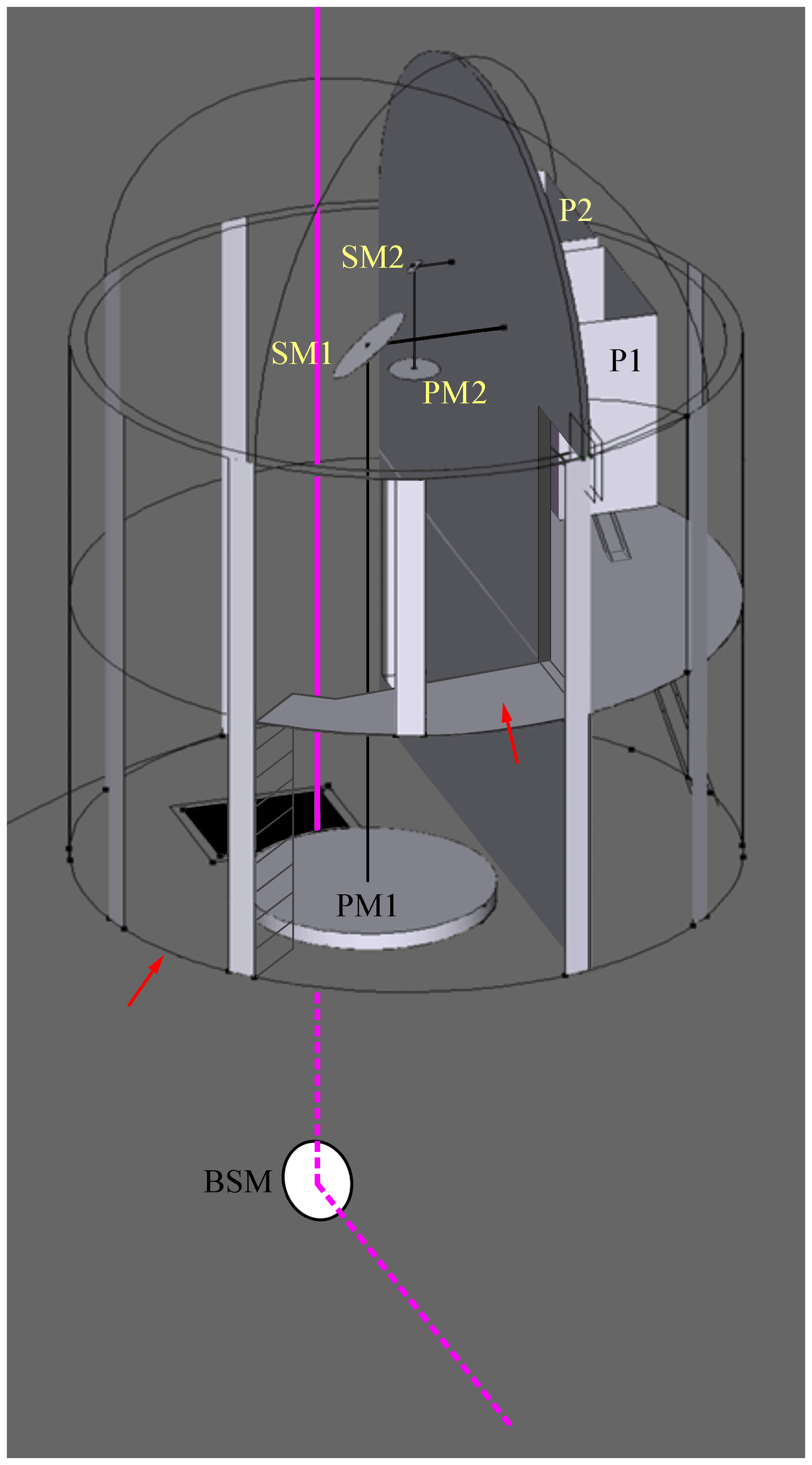
Figure 7 Receiver tower mounted on the terrace above the lidar laboratory. The tower is covered by a 4.2 m diameter astronomical dome with a 1.5 m slit. The laser beam (violet) emerges from a former emergency shaft. The plane formed by the axes of the large telescope and the laser beam contains the section of the laser beam in the lower floor. This plane is perpendicular to the plane formed by the axes of the small telescope and the laser beam. Abbreviations: BSM: beam-steering mirror; PM: primary mirror; SM: secondary mirror; P: Polychromator; 1, 2: belonging to far-field receiver, near-field-receiver, respectively. The two red arrows indicate the two entrances of the tower.

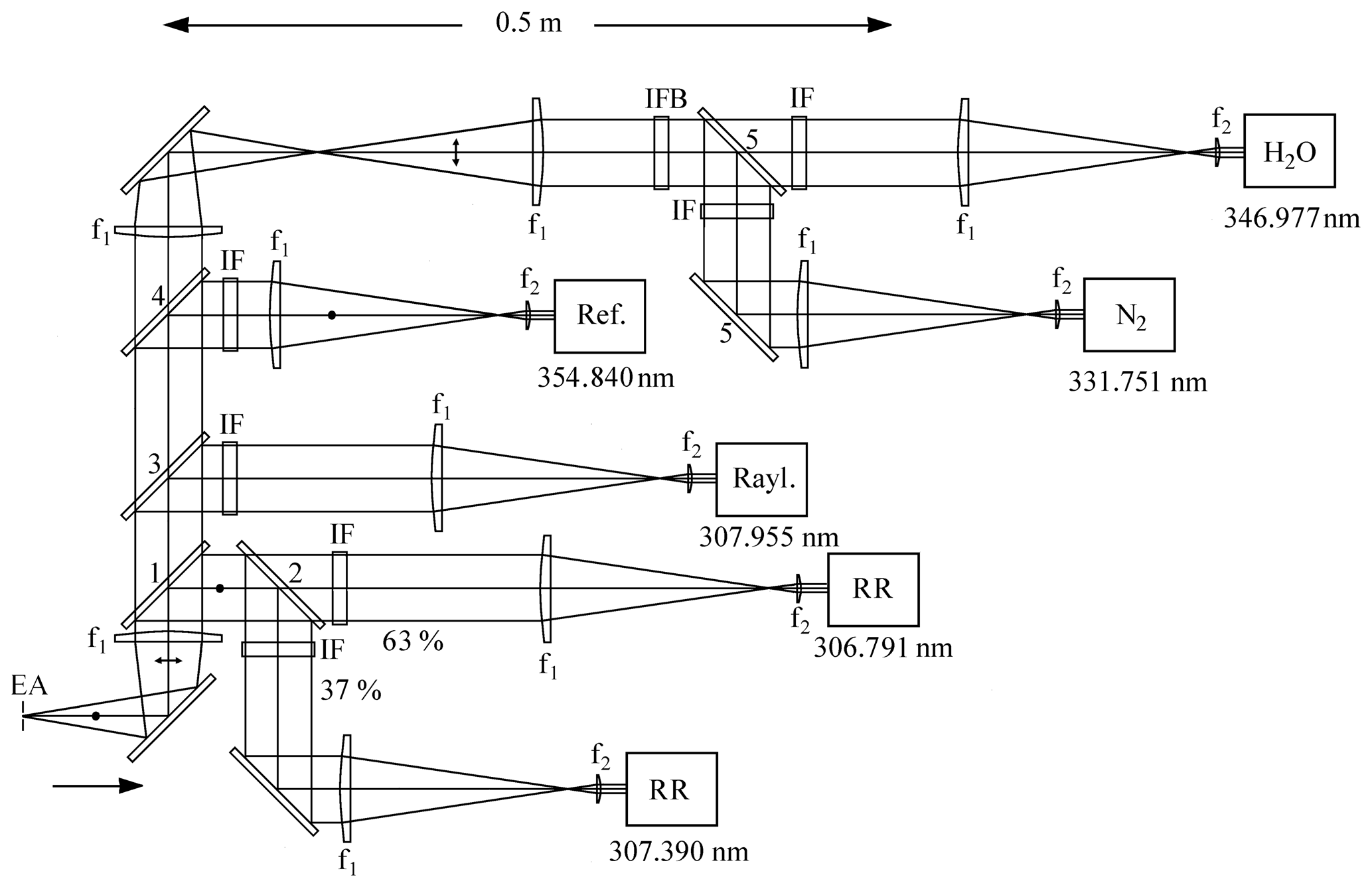
Figure 8 Final polychromator design. The true orientation of the mounting plate (vertical) is rotated clockwise by 90^∘. The radiation cone from the telescopes (arrow) enters the polychromators from behind the plate as indicated by the polarization dot next to the arrow. In detail, EA: entrance aperture with four adjustable blades (OWIS); 1: beam splitter, transmitting almost all P-polarized radiation (308–355 nm) and highly reflecting the S-polarized 308 nm radiation; 2: 63 %∕37 % beam splitter for S-polarized 308 nm radiation; 3: beam splitter reflecting all radiation at 308 nm and transmitting 83 %–91 % of the longer wavelength P components; 4: polarizing beam splitter; 5: sharp-edged long-pass filter for P polarization, reflecting about 99 % at 332 nm and transmitting 99 % of the longer wavelength components ; IF: narrowband interference filters; IBF: broadband interference filter transmitting between 330 and 355 nm with T = 85 %–90 % and blocking the radiation outside this range by at least 10⁵; lenses: f₁ = 150 mm and f₂ = 18 mm (large telescope), f₂ = 30 mm (small telescope). Detailed specifications are given in Table 3.

4.2 Telescopes

Two separate Newtonian telescopes are used with focal length f = 2.0 m and diameter d = 0.38 m (Intercon Spacetec), taken from our former eye-safe aerosol lidar (Carnuth and Trickl, 1994; Trickl, 2010), and with f = 5.0 m, d = 1.50 m (Astrooptik Philipp Keller), respectively. The large focal length of the far-field telescope necessitated installing the receiver system in a separate tower on the terrace above the lidar (Fig. 7). The tower (Sirch and Hägele&Böhm) is covered by a 4.2 m diameter astronomical dome with a 1.50 m slit (Baader Planetarium) which proved to be an adequate solution under the arctic conditions on the high mountain. The entire structure is designed for withstanding wind speeds of up to more than 300 km h⁻¹. The costs for the dome limit its size, and the slit width determines the width of the large telescope. Tower and dome were transported to the site by a big Kamov double-rotor helicopter (HELISWISS), the large mirror with a small helicopter from Heli Tirol. The mirror was lowered to the terrace, from where it was moved into the tower under assistance of two provisional cranes.

Although the frame of the large telescope is prepared for heating, this turned out to be unnecessary because of a powerful heating system inside the tower. The tall frame carries both the secondary mirrors and the two polychromators without contact to the measurement compartment that is stepped on by the operators. The tower can be entered by two doors at the terrace level and upstairs. The upper door allows us to access the measurement compartment directly or to use the emergency exit also after major snowfall.

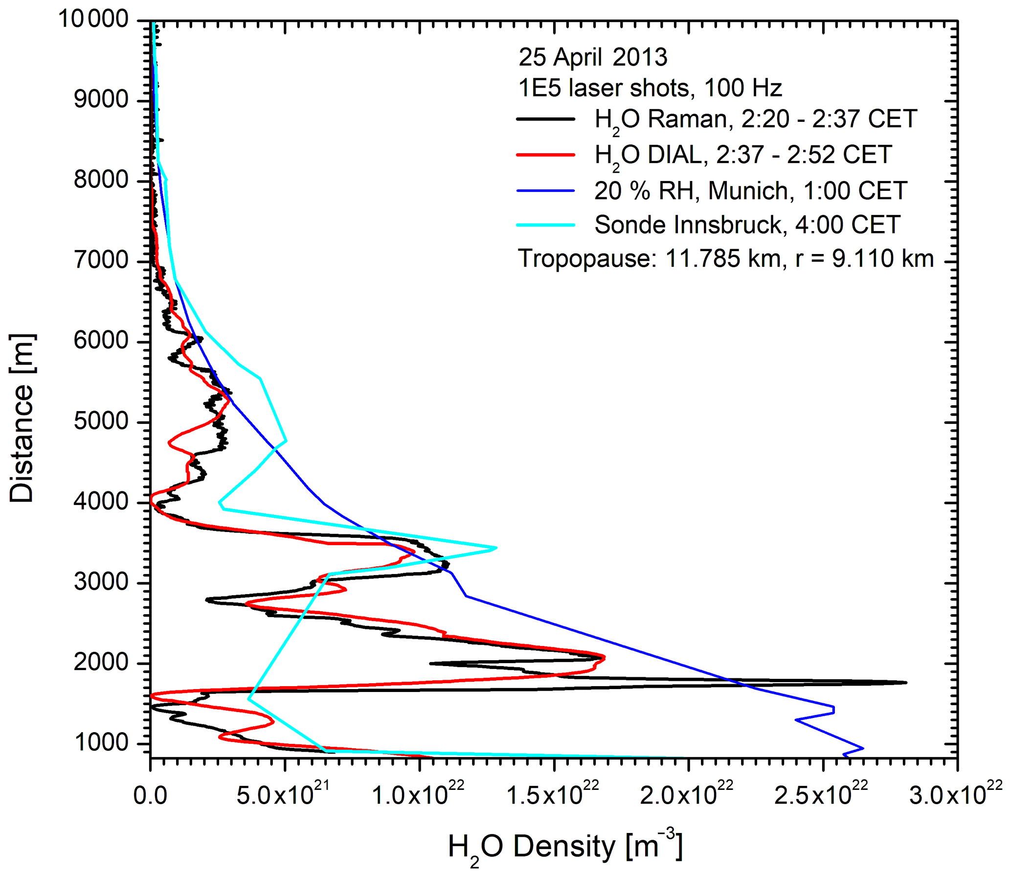
Figure 9 Comparison of consecutive measurements of the Raman lidar and DIAL at UFS on 25 April, 2013: the sonde measurements at Munich (not shown) and Innsbruck strongly differ from those of the lidar systems. For comparison, we show the densities corresponding to 20 % RH as calculated from the Munich radiosonde.

4.3 Polychromators and wavelength separation

The final design of the polychromators is shown in Fig. 8. The optical table (OPTA G.m.b.H.) is in reality oriented vertically, with the left-hand side representing the top. The entrance of the radiation arriving from the telescope is horizontal (see Fig. 9), i.e. rotated with respect to the drawing plane, as one can see from the change in polarization vector (dot for out-of-plane to double arrow for in-plane orientation). The radiation bundle is spatially filtered with a rectangular aperture with four adjustable blades (custom-made by OWIS) placed in the focal plane. Due to space limitations, the aperture is oriented perpendicularly to the beam axis. A slight tilt angle would be superior because of the longitudinal walk of the “focus” (Trickl et al., 2020b). This will be made possible in the future by mounting additional inclined apertures in front of the PMTs. In this way, the different diameters of the focal points, caused by the different beam divergences of the two lasers, can also be accounted for.

Several relay-imaging modules formed by confocally arranged f = 150 mm lenses (f₁) are seen (Sect. 3.1; see also Vogelmann and Trickl, 2008). In the sections with parallel beams (with one exception), beam splitters and interference filters are placed in or close to image planes of the primary mirror. Another confocal pair of f₁ lenses (not shown) is used to transfer the radiation from the focus of the large telescope to the first focal point in the polychromator. The short-f lenses (f₂) image the principal mirror on to the photocathode of the photomultiplier tubes (PMTs). The exact positions of the intermediate and final exit pupils can be nicely identified with visible sky light after removing the interference filters.

Table 2 Receiver details.

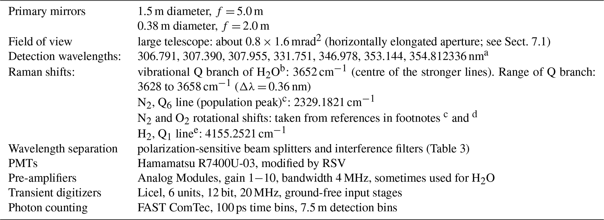
^a Measured during the project by Vogelmann and Trickl (2008). ^b Avila et al. (2004). ^c Trickl et al. (1993, 1995). ^d Rouillé et al. (1992) and Golubiatnikov and Krupnov (2004). ^e Bragg et al. (1982) and Dickensen et al. (2013).

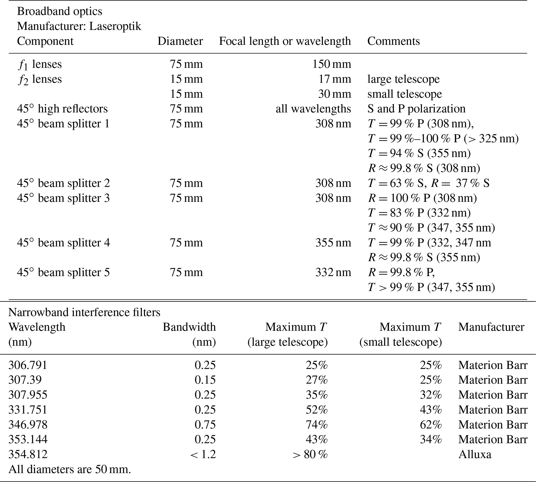
The specifications of the polychromators are listed in Table 2, including the lidar vacuum wavelengths and the Raman shifts used. The Raman shifts in Table 2 sometimes differ from those in the lidar literature. The radiation for the different wavelengths is separated by dichroic beam splitters and narrowband interference filters. This is a highly demanding task considering the 8 to 10 orders of magnitude in signal between the Rayleigh and Raman channels (Sect. 4.3). Figure 8 shows the principal polychromator design without the black walls separating the detection compartments or surrounding the filters. In order to save costs, the optics of both polychromators are equal for except for focal length f₂ that is chosen to achieve image diameters of the order of 5 mm for the different primary mirrors.

The optics (Table 3) were mostly purchased from Laseroptik G.m.b.H., with the exception of the narrowband interference filters and the steep-edge long-pass beam splitter 5 (Materion Barr). The width of the interference filter for water vapour (347 nm) was chosen to cover the entire rather wide Q branch of H₂O in order to avoid a temperature influence on the backscatter profiles. A broadband interference filter (IFB; Semrock; T = 85 %–90 %) was recently added for additional suppression of a potential residual influence of radiation outside the wavelength range of the Raman returns such as scattered light from illuminations inside the laboratory, from the buildings of the ski area or residual 308 nm contributions.

The design in Fig. 8 differs for the two long-wavelength channels from that described by Klanner et al. (2012), used until 2017. The old approach to separate the 347 and 353 nm returns was based on a pair of beam splitters with a steep spectral edge similar to those used for separating the N₂ channel. The perfect separation of the H₂O signal was not possible for maximum suppression of the 353 nm component. Even very small angular changes would imply calibration drifts during routine operation. The modifications in Fig. 8 remove the alignment-dependent signal loss in the H₂O channel. They benefit from the new laser concept (Sect. 3.3): the 355 nm pulses are temporally shifted with respect to those at 308 nm. In this way any residual 355 nm interference in the 347 nm channel is avoided.

4.4 Detectors and discriminators

The detector choice is based on the experience from our stationary ozone lidar system. The final development stage took place parallel to that for the ozone DIAL and is described in detail in Trickl et al. (2020b). Hamamatsu R7400U-03 tubes were chosen and integrated into an actively stabilized socket optimized for us in 1999 for our three-wavelength aerosol lidar by Romanski Sensors (RSV). The socket is now modified to deliver optimized single-photon spikes without the ringing of the original PMTs that had previously enhanced the count rate in our ozone DIAL up to about 5 km. Signal-induced non-linearities can be avoided for normal operating voltages around 800 V if one limits the analogue signal to roughly 100 mV or less. This level is high in comparison with traditional PMTs. Non-linearity in the photon-counting signal was revealed by a comparison with a simultaneous ozone measurement at Hohenpeißenberg for analogue signals of 400 mV.

The output of a PMT is fed into an impedance-matched junction containing the discriminator (also from RSV). The output for the analogue channel is slow, with single-photon pulses widened by a factor of 2. The second branch is the fast discriminator that emits −0.4 V constant amplitude pulses with a full width at half maximum of 0.6 to 1.5 ns, depending on the photon pulse height. The discriminator level that can be chosen from −2 mV to lower voltages is important for the six-dynode PMT and its rather small pulses. The pulse–height distribution for 800 V shows pulses from −2 to −23 mV and peaks at about 10 mV (Trickl et al., 2020b). We have applied discriminator levels between −4 and −5 mV.

An important issue for achieving a high sensitivity is a low level of dark-count photons, which normally requires cooling of the PMT (0.03 counts s⁻¹; Trickl and Wanner, 1981). With the PMTs used here and discriminator levels of −4 mV, no dark count was registered in 50 ns bins within 1 h (1 × 10⁶ laser shots) without cooling. The average external background for atmospheric measurements is clearly less than 1 count for voltages up to the maximum of 1000 V, except for the H₂O channel (see Sect. 7).

Table 3 Specifications of the polychromator optics.

4.5 Transient digitizers

Following the other lidar systems developed at IFU since 1995 we purchased two 12 bit, 20 Hz transient digitizer systems from Licel, each with six channels. Licel designed new, ground-free input amplifiers for this project and the ozone DIAL . This latest version has led an unprecedented performance in the ozone DIAL, with a relative noise level of about ± 1 × 10⁻⁶ of the full voltage range after minor smoothing, also yielding highly sensitive aerosol measurements at 313 nm despite the short wavelength (Trickl et al., 2020b).

An exponentially decaying contribution of roughly 10⁻⁵ of the peak signal is present that scales with the signal pulse area; i.e. it grows with the wavelength. After introducing the discriminator for the photon-counting channel and the counter, the exponential wing increased and a slight undershoot occurred in addition. The interference could be strongly reduced by adding an optocoupler to the trigger input of the counting system (Sect. 4.6). Some more sophisticated impedance matching is necessary for achieving an ultimate performance. Examples of the performance achieved so far are shown in Sect. 7.

Another limitation has resulted from the high data transfer produced by the chosen 16 000 bins (120 km): the repetition rate of the laser had to be limited to 300 Hz in order to allow for a reliable data storage.

4.6 Photon counting

Single-photon counting is mandatory in a lidar system with stratospheric capability. In order to benefit from the temporal resolution of the PMTs, we purchased MCS6 and one MCS6A five-channel photon-counting systems from FAST ComTec. Just two of them were used in the end since the analogue signal range for the near-field receiver was found to be good enough to do without photon counting. The signals are scanned for falling edges at intervals of 100 ps, which means a maximum count rate of about 5 GHz for equidistant picosecond pulses.

A bottleneck of this counting system is the sequential data transfer to the computer that limits the signal to 1.8 × 10⁷ s⁻¹. The multi-channel scaler was, therefore, triggered with a delay of 10 to 20 µs with respect to the laser pulse, which resulted in a fully linear performance for H₂O. However, if an earlier beginning of the individual measurement is desired, on-board averaging becomes necessary, which is not implemented in this model. Another limiting issue has been the control program of the counting system: an automatic start from outside UFS is not reliable, and, thus, a mouse click on the “start” symbol is needed on the remote computer.

4.7 System control

The electronic components of the two DIAL systems (Ingenieurbüro W. Funk) are ground-free. The trigger pulse is derived from a photodiode and subsequently distributed into numerous output channels via optocouplers. The supply voltages are transferred to the different devices in shielded cables. The shields of the cable leading to the PMTs are open on the side of the detectors. The supply voltage can be set by the lidar PC via an I²C bus. Electromagnetic interference in the lidar signals from outside (e.g. the laser) has been kept at a negligible level by using doubly shielded cables (Suhner, G03332; the outer shield is left open on one side) and ground-free circuits.

The data acquisition of the lidar system is controlled from a central Linux computer via a Perl program and Ethernet. The Licel transient digitizers are fully read every 10 s. At a repetition rate of 300 Hz this allows for an integration without overflow due to the 24 bit depth for each unit. This data stream is subsequently integrated for each channel by the controlling program until the end of the measurement after 1 million laser shots, corresponding to an integration time of roughly 1 h. The measurement data are finally stored in an ASCII file, including meta information in the file header.

The same Perl program is designed to control also the photon-counting devices via Ethernet communication with the Windows-based FAST ComTec software. As mentioned, this communication does not yet work reliably for control from outside UFS.

Meanwhile, the excimer laser can be operated via Ethernet, as well as the rotation of the etalon, the spectrometer HR400 and a new motorized end mirror of the XeCl laser. The laser power supply and cooling water pump are controlled by Wago-SPS units (programmed in CodeSys) via a Java web interface. The beam-steering mirror is motorized and remotely controlled by custom-made software from ASA. The slit of the lidar dome, the covers of the telescopes, the laser output mirror and the power supply of the lidar receiver are controlled with a Wago-SPS system via a Java web interface.

5 Data processing

5.1 Reference data

Apart from the water-vapour DIAL, we use meteorological data from different sources as external references. Up to typically 32 km, we take radiosonde data from the sounding stations nearest by, Munich (Oberschleißheim; 101 km roughly to the north), Hohenpeißenberg (42 km to the north) and Innsbruck (32 km to the south-east). Up to a geopotential altitude of roughly 54 km, we import data from NCEP (National Centers for Environmental Prediction; http://www.ncep.noaa.gov/, last access: 20 January 2020). The NCEP values are calculated daily for all NDACC stations. Beyond this, initial density and temperature guesses are derived from the U.S. Standard Atmosphere (1976). For all reference data the geopotential altitudes are converted into real ones.

5.2 Water vapour

A great advantage of Raman lidars is that uncalibrated H₂O densities are obtained in a robust way by multiplying the backscatter signal for the full ro-vibrational Q branch by the square of distance r (range correction). Thus, small perturbations of the signal do not matter as severely as in the DIAL algorithm that implies derivative calculations. However, in our system, the choice of a particularly powerful UV laser implicated a short operating wavelength of 308 nm. Thus, for obtaining number densities, an ozone correction must be made that is based on the DIAL solution for the wavelengths 307.955 and 353.11 nm (or recently 354.22 nm).

For simplicity we have so far preferred calculating just water-vapour volume mixing ratios, which also makes a range correction superfluous. The uncalibrated mixing ratios are calculated by dividing the H₂O backscatter signal by the vibrational nitrogen Raman backscatter signal. Here, the influence of ozone is cancelled out on the upward path exactly because the transmitted wavelength is the same for both Raman channels. On the downward path, a small residual absorption in the stratospheric ozone exists at 331.75 nm that grows to almost 2 % at 20 km and has been neglected given the current level of accuracy at this altitude. The photon-counting data are collected at 51.2 ns per bin instead of the 50 ns in the transient digitizers and are interpolated to match the timescale of the analogue data. In order to avoid excessive data array sizes, we double the bin size to 100 ns during the subsequent calculations, averaging pairs of neighbouring signals.

In the useful range for H₂O up to roughly 20 km, the relative noise of the nitrogen Raman signal is negligible, and no smoothing is applied. Smoothing is just applied to the Raman signal ratios that are determined separately for the analogue and the photon-counting data. The smoothing approach is based on a numerical low-pass filtering approach with a Blackman window, described and characterized in the parallel paper by Trickl et al. (2020b). This numerical filtering approach is free of ringing. The filtering interval is dynamically increased. As shown in Sect. 6, a purely quadratic dependence

$$L=\mathrm{1.2}\times {\mathrm{10}}^{-\mathrm{4}}{i}^{\mathrm{2}}$$

as a function of 15 m bin i (minimum interval size: 2 bins, i ≤ 300) (or slightly modified for noisier data) is adequate. In one case (5 February 2019) a third-order polynomial was used for L to achieve a better vertical resolution in the lowermost stratosphere in the presence of a steep concentration feature. In a Raman lidar this dependence does not require much modification from measurement to measurement, whereas in a DIAL, the strongly changing water-vapour concentration results in considerable change in absorption and, thus, of the smoothing requirements. The definition of vertical resolution so far used by us is given by the range interval corresponding to the 25 % to 75 % rise of the response of the smoothing filter to a Heaviside step (VDI, 1999). For the Blackman filter the VDI vertical resolution is 19.3 % of the size of the smoothing interval. Leblanc et al. (2016) recommend defining the vertical resolution as the full width at half maximum of a delta response, which is 34.7 % of the filtering interval for the Blackman filter. Equation (1) yields a VDI vertical resolution of 155 m at 10 km, 348 m at 15 km and 619 m at 20 km, and a delta-response vertical resolution of 277 m at 10 km, 624 m at 15 km and 1109 m at 20 km.

The role of aerosols is limited to extinction and, in the case of biogenic particles (Immler et al., 2005; Reichardt et al., 2018), to fluorescence in a Raman lidar. The presence of aerosols is best judged from the 355 nm channel. The influence of extinction is very low when calculating the H₂O mixing ratio from the ratio of the H₂O and N₂ profiles. An estimate of the extinction coefficients at the two wavelengths can be obtained from the 355 nm data.

The system testing was limited to clear nights. Thus, aerosol effects could be neglected.

5.3 Temperature

The retrieval of temperature from lidar data is a highly demanding task. For instance, an uncertainty of 1 K means a relative uncertainty of 0.33 % at a temperature of 300 K. Thus, a very high quality of the backscatter signals is a prerequisite for reasonable results. For our system the two conventional methods have been selected, evaluating the temperature dependences of the rotational Raman spectra received just below 308 nm (Arshinov et al., 1983) and the direct retrieval of temperature from backscatter profiles (Hauchecorne and Chanin, 1980).

The retrieval of temperature profiles from rotational Raman backscattering has not yet been optimized and is, thus, not described here. The main problem has been that the first generation of 307.390 nm interference filters obtained from Materion Barr did not sufficiently reject the 307.955 nm contribution. In principle, this contribution is a reasonable reference in the absence of aerosol because it is independent of temperature. Thus, several successful temperature retrievals could be achieved for the near-field receiver (Höveler, 2015).

The evaluation of temperature profiles directly from backscatter profiles has been tested for the Rayleigh channels at 308, 353 and 355 nm, as well as the nitrogen Raman channel (332 nm). Due to the signal losses caused by ozone the range of the N₂ channel is limited. We finally decided to invert the backscatter signal for 355 nm (Sect. 2.3). The analogue and photon-counting backscatter profiles are merged into a single profile, switching at about 28 km. The resulting profile is, again, smoothed with the Blackman filter mentioned above. Similar to water vapour, the filtering interval Δ is enhanced as (approximately)

$$L=\mathrm{2}\times {\mathrm{10}}^{-\mathrm{5}}{i}^{\mathrm{2}}$$

as a function of 15 m bin i.

We follow the strategy of calculating the temperature described by Shibata et al. (1986). In a first step the density is calculated and subsequently the temperature. However, instead of the simplified density algorithm, we use a fully quantitative Klett-type approach with downward integration from the far end (Klett, 1981, 1985). The result is calibrated to the number density n and not to the backscatter coefficient:

$$\begin{array}{}\text{(1)}& n\left(r\right)={\displaystyle \frac{n\left(r_{\text{ref}}\right)r_{\text{ref}}^{\mathrm{2}}S\left(r_{\text{ref}}\right)}{r^{\mathrm{2}}S\left(r\right)+\mathrm{2}n\left(r_{\text{ref}}\right){\mathit{\sigma }}_{\mathrm{R}}\left[\mathrm{1}+\underset{r}{\overset{r_{\text{ref}}}{\int }}{r}^{\prime \mathrm{2}}S\left(r^{\prime }\right)\mathrm{d}{r}^{\prime }\right]}},\end{array}$$

S(r) being the ozone-corrected backscatter signal, r_ref the reference distance and σ_R the Rayleigh extinction coefficient. We take as a first approximation a reference value calculated from the U.S. Standard Atmosphere (1976). The results of the inversion with Eq. (1) are then compared with radiosonde or NCEP values in a low-noise range of the backscatter profile at moderate altitudes. If the agreement in this reference range is not sufficient, n(r_ref) is modified, and the procedure is repeated until agreement is reached. This approach is highly robust, a change in reference value corresponding to an approximate parallel shift of the density curves. For the selection of r_ref, it is advisable to select a position for which the signal S(r_ref) is closest to the average of adjacent data points. In this way, the subsequent correction necessitated by the local data noise is the lowest.

The temperature is subsequently calculated from the density by applying

$$T\left(z\right)=T\left(z_{\mathrm{0}}\right){\displaystyle \frac{n\left(z_{\mathrm{0}}\right)}{n\left(z\right)}}+{\displaystyle \frac{m_{\text{air}}}{kn\left(z\right)}}\underset{z}{\overset{z_{\mathrm{0}}}{\int }}n\left(z^{\prime }\right)g\left(z^{\prime }\right)\mathrm{d}{z}^{\prime },$$

with z being the altitude above sea level, m_air = 28.9644 u (U.S. Standard Atmosphere, 1976; 1 u = 1.6605390 × 10⁻²⁷ kg) the mass of an “average air molecule” and g the gravitational acceleration (Mohr et al., 2014),

$$\begin{array}{}\text{(2)}& g\left(z\right)=g_{\mathrm{0}}{\left({\displaystyle \frac{r_{\mathrm{E}}}{r_{\mathrm{E}}+z}}\right)}^{\mathrm{2}},\end{array}$$

with g₀ = 9.80665 m s⁻¹ and the earth radius r_E = 6356766 m.

Equation (2) immediately shows that selecting z₀ at the upper end of the data evaluation range means a strong decrease with the growing density on the way downward. As a consequence, the second term in Eq. (2) clearly dominates the temperature about 15 km downward from z₀. Here, the number density retrieved in the first step determines the temperature. Any density error critically enters the computation of the temperature. Thus, the range of the temperature retrieval is shorter than that of the density retrieval.

5.4 Uncertainties

Uncertainties u of both water vapour and temperature have been approximated by the expression

$$\begin{array}{}\text{(3)}& u=\sqrt{u_{\mathrm{0}}^{\mathrm{2}}+{\left(u_{\mathrm{1}}{\displaystyle \frac{r^{\mathrm{2}}}{r_{\text{ref}}^{\mathrm{2}}}}\right)}^{\mathrm{2}}+\left(u_{\mathrm{2}}S\right(r){)}^{\mathrm{2}}},\end{array}$$

with coefficients u₀, u₁ and u₂ that are adjusted by comparison with reference measurements as shown in the examples in Sect. 7. The second term in Eq. (3), quadratic in r, reflects the quadratic rise of the noise of the unsmoothed quantities. The reference distance r_ref is chosen at the upper end of the data evaluation range. Through the approach with Eq. (3), considerable computation efforts have been avoided.

6 Calibration of the water-vapour profiles with the DIAL

The calibration of the Raman lidar by the water-vapour DIAL operated in the same laboratory is a unique chance to overcome the restrictions imposed by the sometimes extreme variability of water vapour (Vogelmann et al., 2011, 2015). This variability is caused by a rapid sequence of atmospheric layers of strongly different origin. The humidity varies from very high (origin in the boundary layer) to extremely low (origin in the stratosphere). Our routine measurements since 2007 have revealed that on 84 % of our ozone measurement days, stratospheric influence could be identified in the free troposphere (Trickl et al., 2020a). This leads to a particularly strong modulation of the humidity profile.

In Fig. 9 we show the first example of a comparison between the two lidar systems on 25 April 2013. The measurements took place under highly complex conditions in the presence of three dry layers, two of them clearly related to stratospheric air as a result of the almost negligible humidity. 315 h backward trajectories with the HYSPLIT model (http://ready.arl.noaa.gov/HYSPLIT.php, last access: 20 January 2021; Draxler and Hess, 1998; Stein et al., 2015), run here with reanalysis meteorological data, show a 5 to 7 d descent from altitudes above 9 km over western Canada and more than 10 km above the Aleutian Islands for the layers at 4.2 and 6.7 km, respectively.

This was the only case in our entire test phase in which a slight 308 nm background was superimposed on the signal. This background could be reliably removed by subtracting a very simple exponential curve. After calibration of the data from the Raman lidar with those from the DIAL above 5.5 km, reasonable agreement was found in a major fraction of the free troposphere. However, due to using the same electronics in that early phase, the measurements were not made simultaneously. Thus, a few differences are visible and ascribed to the sometimes extreme spatial and temporal variability of water vapour mentioned above.

The strong variability becomes even more obvious from comparisons with the Innsbruck (shown) and Munich radiosonde (not shown) ascents that differ strongly and do not show similarly dry layers despite similar courses of the trajectories calculated for these sites in comparison with those for the lidar station. This example demonstrates that simultaneous calibration of the Raman lidar with the quality-assured DIAL (e.g. Trickl et al., 2016) is mandatory. Unfortunately, comparisons were no longer possible after 2014 due to permanent laser damage of the DIAL. The development of a new Ti:sapphire laser system with a high repetition rate is underway, and emission was already demonstrated.

The stability of the calibration can be monitored by using the signals of the 308, 332 and 355 nm channels outside ranges affected by aerosol.

During the rest of the test period, in part described in the following, the system was calibrated by comparison with sonde humidity profiles from Munich, Innsbruck and Hohenpeißenberg, selecting sections of the sonde profiles that look the most reasonable. During one night in February 2019, very successful comparisons with a CFH sensor (launched in the valley) were made.

7 Measurements in the atmosphere

After the completion of the lidar systems, testing started in autumn 2012. The measurements demonstrated the perfect suppression of interference from the other channels in the water-vapour channel by spectral filtering and shielding. This achievement implies, according to the simulations in Sect. 5.3, a suppression of more than 9 decades of 308 nm background.

In early 2015, the near-field receiver was also completed and performed well. Even rotational Raman retrievals with a temperature noise level of 1 K were achieved (Höveler, 2015). In addition, single-photon counting successfully entered operation for the far-field receiver but was given up for the small telescope because of the excellent analogue performance. In the following, we show results just for the far-field receiver since a good system performance at high altitudes has been the main goal of this project. The examples were chosen to show the performance under different conditions, such as different levels of background noise and different situations of calibration.

7.1 Water-vapour measurements up to 20 km

7.1.1 1 July 2015

The first, quite instructive measurement demonstrating a detection range up to 20 km was achieved on 1 July 2015 (Fig. 10). Due to a wide entrance slit of the polychromator (about 40 mm × 40 mm to facilitate alignments in the dark), a strong background of 155 photon counts h⁻¹ in 15 m bins occurred that included scattered radiation from the almost full moon. Despite the resulting noise of about ± 25 counts, the background-corrected signal, arithmetically averaged over 51 bins, stays positive to distances of up to 19.7 km (22.4 $\mathrm{km}\mathrm{a}.\mathrm{s}.\mathrm{l}.$).

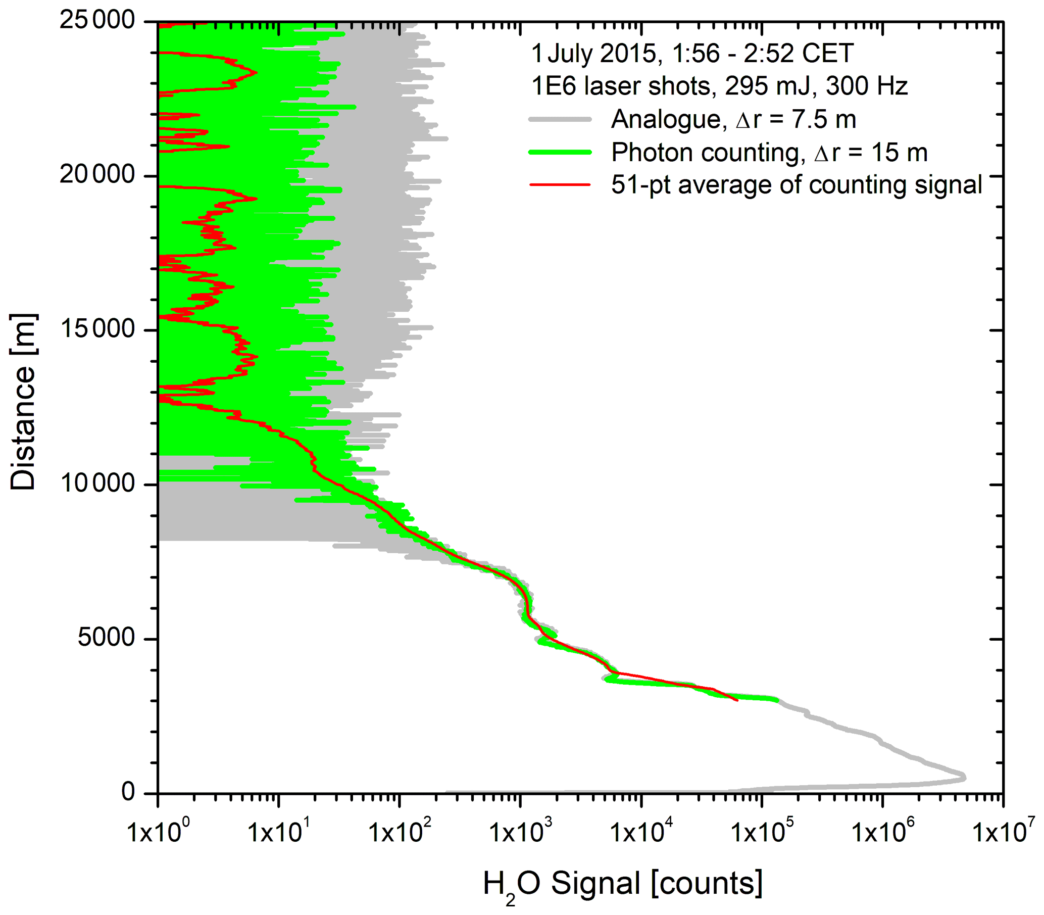
Figure 10 347 nm Raman backscatter signals as a function of the vertical distance above UFS, obtained during the first hours on 1 July 2015. Despite a high noise level of about 12 counts (square root of signal) the averaged signal remains positive up to r = 19.7 km. The averaged signal covers 6 decades, the peak signal being roughly 3 mV. The average laser pulse energy, 295 mJ, was low due to a contaminated cell window.

The signal was accumulated over 1 h with a laser pulse energy of just 295 mJ (300 Hz) due to a dirty window of the laser pump chamber. The analogue signal was corrected, just with a very small exponential decay function, leaving a slight residual signal undershoot at distances around 12 km that is ascribed to the parallel use of analogue detection and photon counting (Sect. 4.4). The peak analogue signal is about 3 mV but is rescaled here to match the counting signal. The photon-counting noise corresponds to an analogue voltage of just about ± 15 nV.

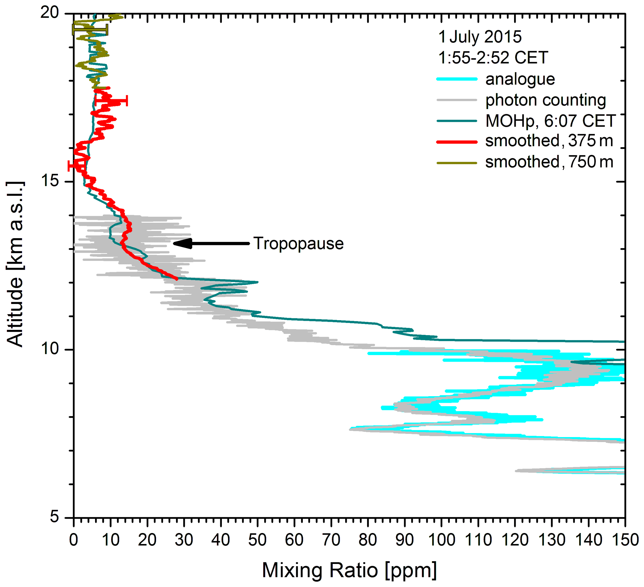
Figure 11 Water-vapour mixing ratio obtained for the measurement in Fig. 11; the calibration is based on looking at zones of best agreement below 7 km between the sonde data for Munich (01:00 CET), Innsbruck (04:00 CET) and Hohenpeißenberg (06:00 CET). Just the Hohenpeißenberg (MOHp) results are displayed here because they agree best with the lidar values above 11 km. 51 and 101 pt arithmetic-means smoothing was applied to the mixing ratios derived from the photon-counting data at high altitudes; the corresponding VDI vertical resolutions are specified in the legend.

The water-vapour mixing ratio is shown in Fig. 11. The calibration of the mixing ratio was very difficult since there was macroscopic mutual disagreement of the lidar and all three Vaisala RS92 radiosonde profiles inspected (Klanner et al., 2018, Fig. 3). A few points below 7 km where the sonde data agree were chosen as reference. The Hohenpeißenberg mixing ratio (early morning) agrees best with the lidar results in the tropopause region and is, therefore, displayed here.

The example of 1 July 2015 is special in our test phase: there was very low water vapour around 15.7 km (about 2 ppm). The drop is verified by the Hohenpeißenberg profile. Although the sonde data become highly uncertain at higher altitudes, we see principal agreement with the lidar. HYSPLIT trajectory calculations indicated advection of tropical air from the Caribbean Sea above the tropopause, slightly downward-shifted, most likely because of the wrong model orography at the northern rim of the Alps. In the tropics, freeze-drying in cirrus clouds has been suggested to lead to dehydration and, thus, low humidity (see Sect. 1). Such an inhomogeneity is a strong motivation for lidar work that features a potential for a good time resolution. Water vapour is an excellent tracer for troposphere–stratosphere transport (TST), and there is some hope that we can study some cases of TST in the future.

7.1.2 Measurements since 2018

The measurements since 2018 have been carried out with full optical insulation of the channels including the covers of the polychromators, with a narrow entrance slit and with measurements at 355 nm with the separate Powerlite laser. In 2018 and until 6 February 2019, a total of 14 1 h measurements and several shorter tests were carried out during nights that were completely cloud-free. The minimum H₂O mixing ratios were 4 to 6 ppm, i.e. in the range one would expect for the stratosphere from the literature cited in the Introduction.

The smallest slit size tested was roughly 2 mm × 8 mm. The horizontal elongation allows the slightly inclined near-field return to enter the polychromator. This size led to one to two background counts per 7.5 m bin and 1 h but also to an indication of a lower backscatter signal. This behaviour is in agreement with the large beam diameter in the focal plane of roughly 2.5 mm expected from the laser beam divergence and the receiver focal length of 5 m. The final chosen size of the horizontal entrance slit was roughly 4 mm × 8 mm, resulting in 3 to 5 background counts.

The reason for the background counts in the water-vapour channel could not be fully clarified. Upper atmosphere air-glow spectra (Broadfoot and Kendall, 1968; Johnston and Broadfoot, 1993) show several features in the wavelength range of the lidar return for λ ≥ 332 nm. However, some spectral overlap also exists with the components at 332, 353 and 355 nm, where the measured background is very low.

7.1.3 19 July 2018

During the early hours of 19 July 2018, two subsequent measurements were made that could be compared. The average laser pulse energy was just 380 mJ (300 Hz). The background count rate was 5–8 counts h⁻¹ per bin for a slightly larger entrance slit.

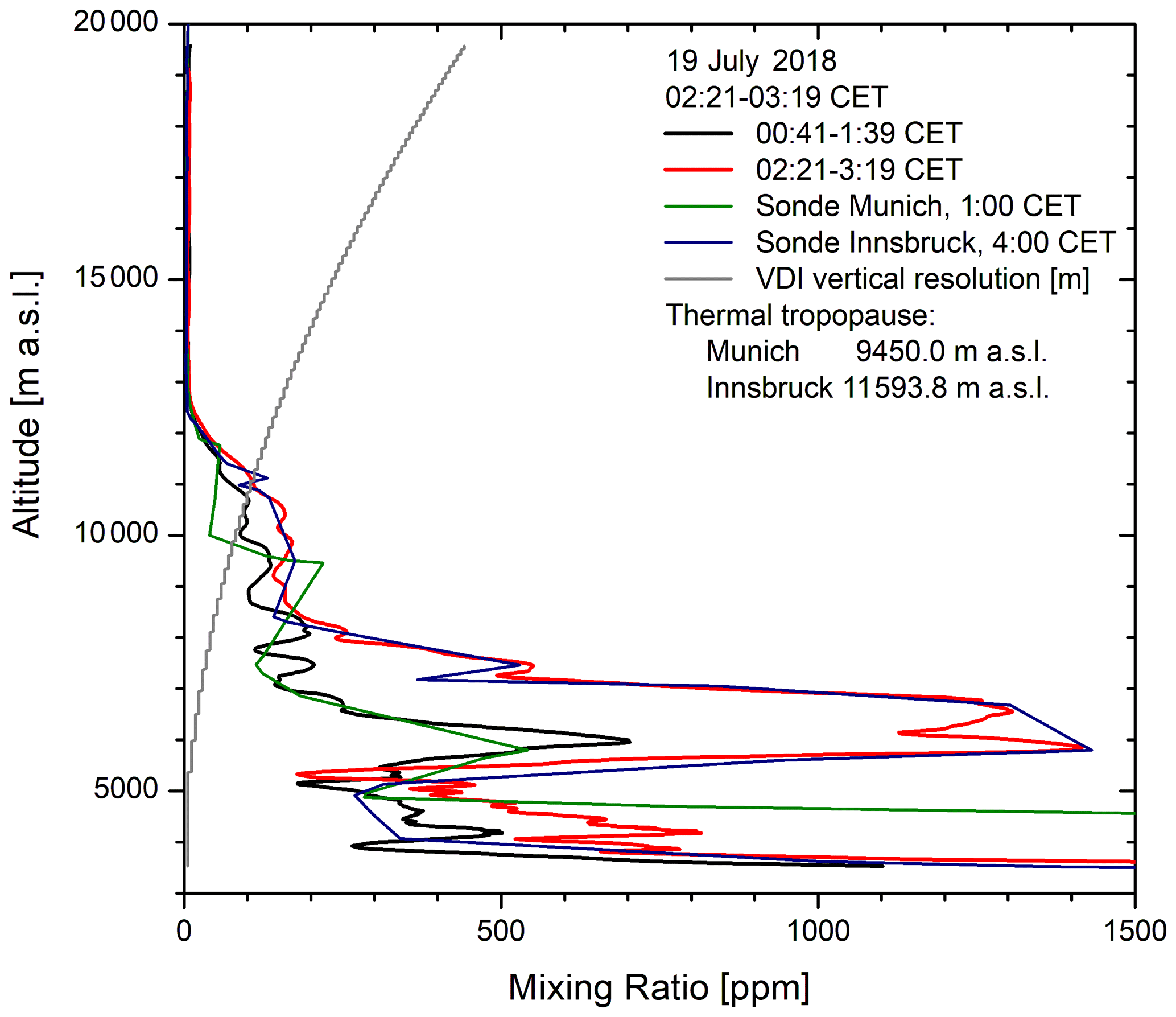
Figure 12 Calibration of the measurements on 19 July 2018: the profile derived from the first measurement agrees better with the 01:00 CET sonde data from Munich. The mixing ratios for the second measurement almost coincide with those from the later sonde launch at the airport of Innsbruck. The average laser pulse energy was 380 mJ (300 Hz).

The mixing ratios obtained are shown in Fig. 12. The calibration of the first measurement was estimated from the Munich sonde data for the launch at 01:00 CET. The profile for the second measurement looks completely different, which, again, demonstrates the strong atmospheric variability of water vapour. Here, the calibration of the lidar mixing ratios was based on the Innsbruck sonde (nominal daily launch: 04:00 CET). We assume that the horizontal homogeneity is much better in the tropopause region, where we, thus, centred the calibration. However, the agreement is also reasonable around 6.5 km (5 % to 10 %).

The two profiles for the lidar agree quite well up to about 18 km (Fig. 13), despite the elevated signal background. The second measurement was noisier, which is reflected by the larger error bars.

It is interesting to note that the sonde data are substantially lower than the mixing ratios from the lidar, which is also the case in the following examples. We speculate that this is due to a change in sonde type from RS92 to RS41 by the German Weather Service. We have found that the RS92 data are highly realistic in our tropospheric studies in comparison with our DIAL (Trickl et al., 2014–2016). For 2018, the data for the new sonde type exhibited a positive bias of 2 %–3 % relative humidity (RH) in intrusion layers.

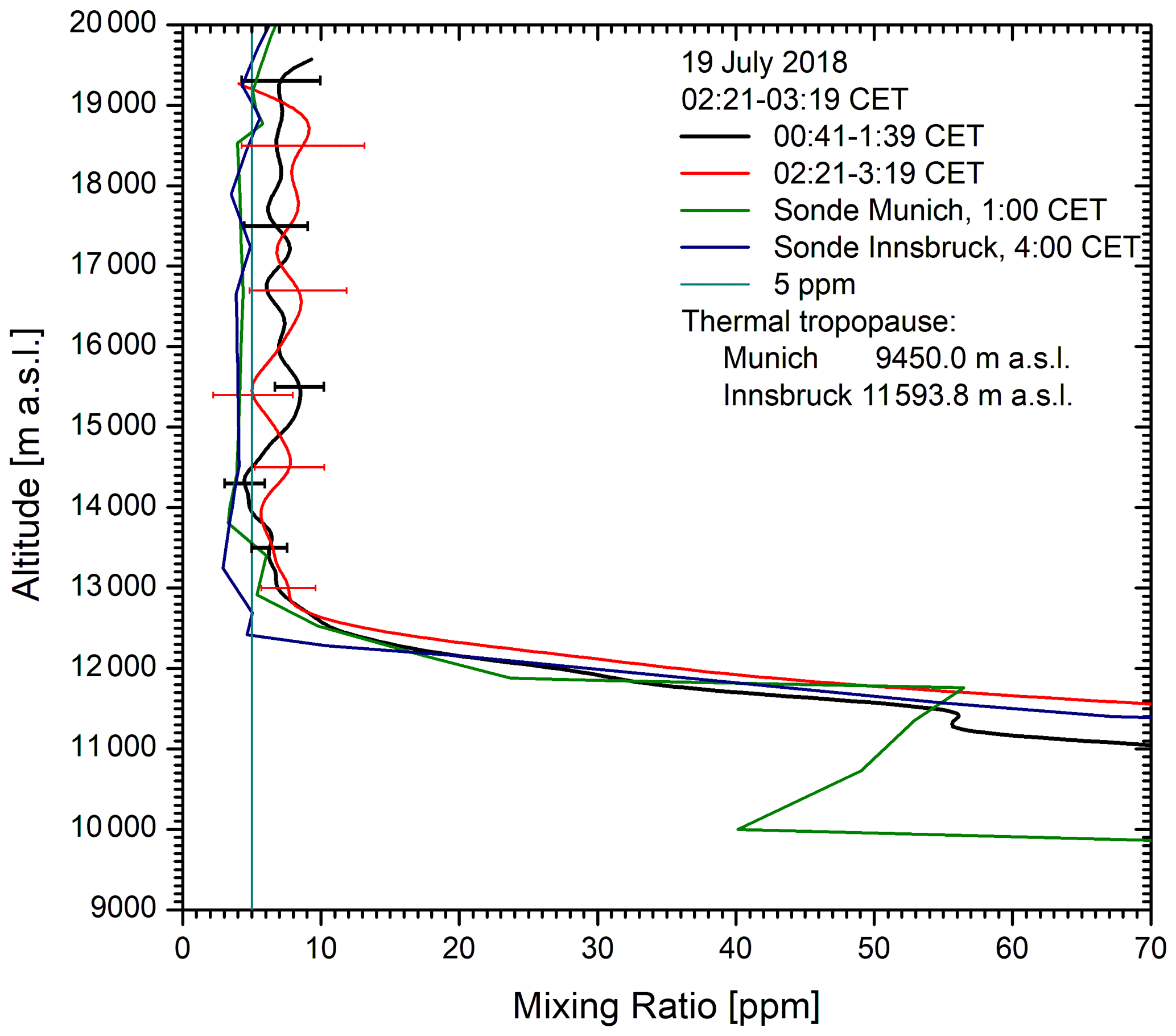
Figure 13 Comparison of the two lidar measurements on 19 July 2018, and the Innsbruck sonde on a close-up scale: the lidar values agree well up to 18 km, ranging between 5 and 12 ppm. The mixing ratio for the radiosondes (presumably RS41) is much lower than that for the lidar in the stratosphere.

7.1.4 5 February 2019: system validation

On 5 and 6 February 2019, several balloons with cryogenic frost-point hygrometers (CFHs; Vömel et al., 2007; 2016), standard Vaisala RS41-SGP radiosondes, ECC ozone sondes (Smit et al., 2007) and COBALD backscatter sondes (Brabec, 2011) were launched in the valley at IMK-IFU (9 km to the north-east of UFS) by a team of the Forschungszentrum Jülich. The data were transmitted to a ground station installed for this campaign at the Zugspitze summit. The combined balloon payload is well tested and also regularly used by the GCOS Reference Upper Air Network (GRUAN) (e.g. Dirksen et al., 2014).

The CFH has an uncertainty of about 2 %–3 % in the troposphere and less than 10 % in the lower stratosphere. Thus, the CFH is especially suitable for measuring water vapour under the dry conditions at the tropopause and in the stratosphere up to altitudes of 28 km.

The first night of the campaign was clearer, and these results are presented in the following. The conditions for the comparison were excellent: the sondes rose almost vertically up to 8.5 km and then slowly drifted to the south-east (Innsbruck). The balloons stayed within 20 km distance of IMK-IFU up to the tropopause (12.8 $\mathrm{km}\mathrm{a}.\mathrm{s}.\mathrm{l}.$) and remained within 30 km up to 20 $\mathrm{km}\mathrm{a}.\mathrm{s}.\mathrm{l}.$

The launch times of the balloons were 18:03 CET (ascent to 16.147 km), 19:03 CET (29.475 km) and 23:00 CET (29.469 km). The profiles of the CFH H₂O mixing ratio during that period mutually agreed to within 0.5 ppm between 13.0 and 17.5 km and slightly more up to 26 km. Just two of the three lidar measurements at UFS cover the full standard measurement time of 1 h and are presented here.

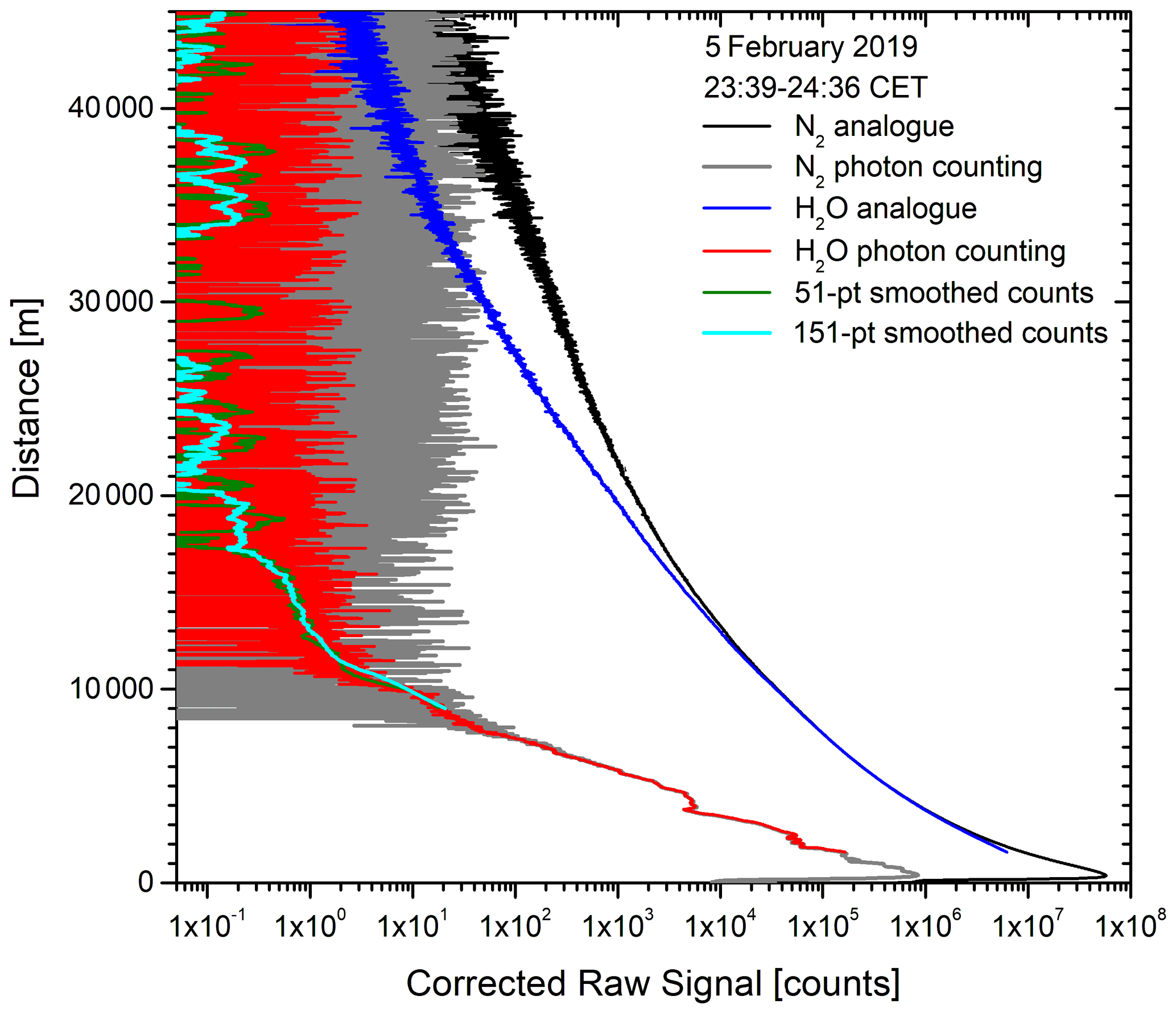
Figure 14 Nitrogen and water-vapour backscatter signals on 5 February 2019 as a function of the vertical distance above UFS; The H₂O backscatter profiles averaged over 151 7.5 m bins (i.e. raw data; VDI vertical resolution: 562.5 m) become noisy at about 17 km (19.7 $\mathrm{km}\mathrm{a}.\mathrm{s}.\mathrm{l}.$). The laser pulse energy was just 360 mJ (300 Hz).

The H₂O Raman backscatter profile for the measurement before midnight is shown in Fig. 14. Due to a narrow slit, the H₂O raw data exhibit an average background of just 2.33 counts (subtracted here), with a SD of 1.55 counts. Two curves with gliding arithmetic means over ± 25 and ± 75 bins are included that suggest a useful range up to r = 17 km (h = 19.7 $\mathrm{km}\mathrm{a}.\mathrm{s}.\mathrm{l}.$). The remarkably low sensitivity limit for the averaged curve corresponds to roughly 0.1 nV analogue voltage. The dynamic range within the dry free troposphere and the lower stratosphere covers an astonishing 7 decades.

The nitrogen Raman backscatter signal is considerably larger. Thus, the onset saturation effects can be seen in the photon-counting data below r = 4 km. Here, the analogue data are, still, valid for at least two more downward kilometres. The analogue signal starts to deviate from the photon-counting signal due to an exponential decay in the signal processing mentioned in Sect. 4.5. We do not correct this effect because the photon-counting method is used at high altitudes.

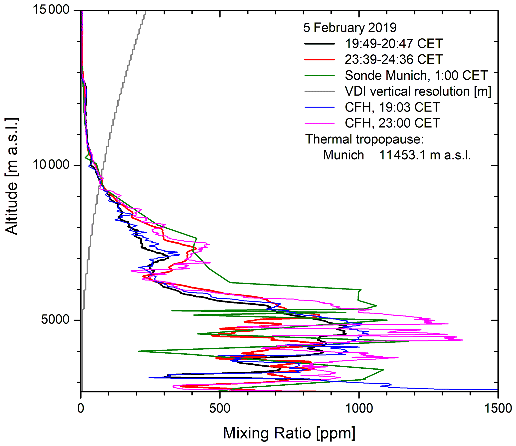
Figure 15 Vertical distributions of water vapour derived from two measurements of the Raman lidar on 5 February 2019 together with those from the midnight Munich sonde and the CFH sensors; the CFH data in the upper troposphere were used for calibration.

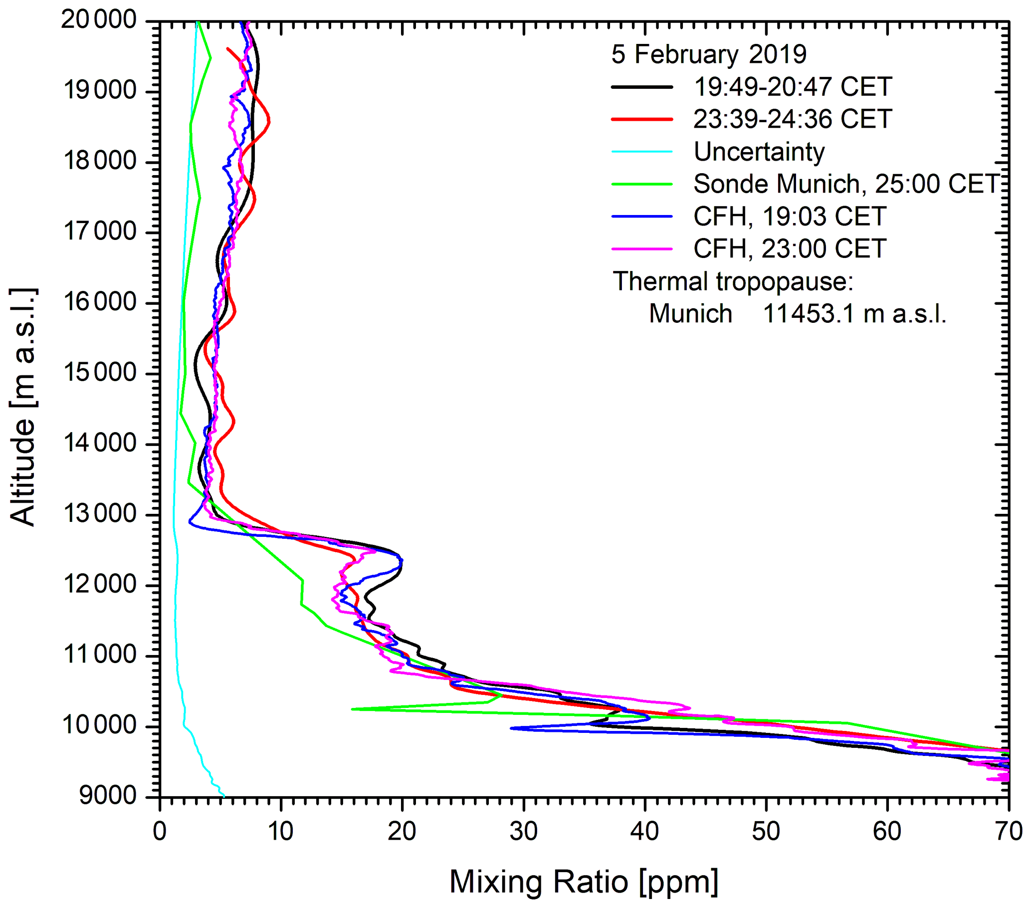
Figure 16 A close-up portion of Fig. 20: the agreement between the lidar and the CFH is satisfactory up to almost 20 km. Above this, the lidar values start wider excursions around the CFH mixing ratios.

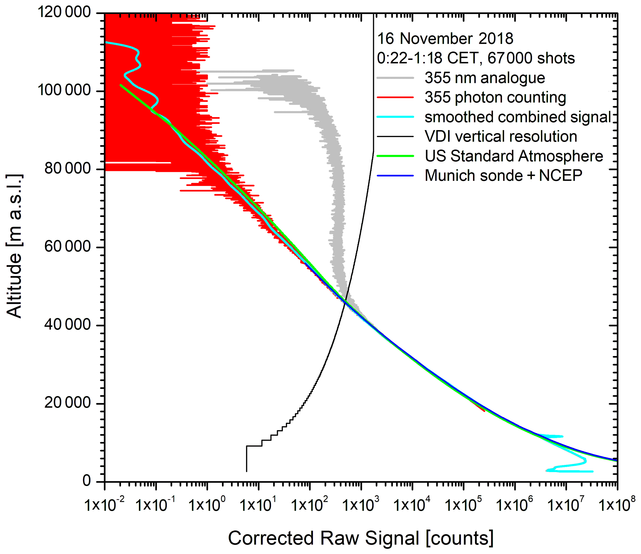
Figure 17 355 nm backscatter coefficients for a 355 nm measurement on 16 November 2018 together with the smoothed combined analogue plus photon-counting signal; the VDI vertical resolution of the smoothing procedure is given in metres. Simulated backscatter signals calculated from the U.S. Standard Atmosphere (1976) and a combined radiosonde and NCEP profile are included for comparison.

Figures 16 and 17 show the water-vapour mixing ratios obtained for two measurement periods on 5 February with 1 h lidar measurements together with those from the almost simultaneous CFH ascents. In addition, the values for the Munich radiosonde (6 February, launched at 01:00 CET) are included for comparison. The grey curve corresponds to the VDI vertical resolution used for the numerical filtering that is about 0.2 km at 14 km and 0.47 km at 20 km. Due to the moderate smoothing around 13 km, the downward humidity step at 12.8 km is just slightly widened with respect to the CFH sensor. We reduced the vertical resolution of the first measurement around this step by introducing a third-order dependence (polynomial) of the smoothing interval (Eq. 1) but could not improve the steepness of this step. We conclude that the width of the step in the lidar result is primarily determined by the long data acquisition over 1 h.

The lidar was calibrated in the upper troposphere above 7.7 km, yielding an almost perfect agreement with the CFH measurements in this range. Between 7.7 and 5.7 km, it is still satisfactory, with a deviation of 5 % to 10 %. Below this altitude, the agreement for the first profile was also acceptable, the lidar value lying in the middle of the CFH mixing ratios for ascent and descent (the latter not shown for clearness). This was quite different for the second profile recorded before midnight when the atmosphere was obviously highly inhomogeneous in space, even on a horizontal scale of 10 km given by the almost vertical rise of the balloon. The presence of several very thin dry layers, also over Munich, indicates a pronounced filamentation.

Below this zone, the agreement is good for both measurements. This indicates a good cancellation of the overlap functions of the nitrogen and water-vapour channels, similar to DIAL systems.

7.2 Temperature measurements

7.2.1 Rotational method

A few measurements based on the rotational temperature method were evaluated for the near-field receiver (Höveler, 2015). The Cabannes influence was corrected for. A good performance with a temperature noise of less than 1 K in a range up to 8 km in the free troposphere was achieved. With recently purchased new narrowband interference filters (Materion Barr rejection of Cabannes radiation to 2 × 10⁻⁴) and a better polarizing beam splitter (Laseroptik, T > 99 %), we expect a much better rejection of the Cabannes radiation.

7.2.2 Rayleigh method

Temperature profiles based on the Rayleigh approach have been made for the wavelengths 308, 332, 353 nm and, finally, 355 nm. For 308 and 332 nm, the signals must be corrected for the absorption of the radiation in ozone. The range for 332 nm ends far below the mesosphere and is, therefore, no longer considered. For 308 nm, a temperature retrieval up to 55 km was achieved. However, the backscatter signal was attenuated with a neutral-density filter by a factor of 1000 in order to avoid detector overload. This means that, without attenuation, a high-speed chopper must be added to cut off the signal returning from the first 10 km. Then, the performance could be excellent. The 353 nm channel was successfully tested at low repetition rates (yielding reasonable temperatures up to 52 km) but was given up because of the loss of Raman conversion at full power.

Here, we present the first demonstration of a measurement with the separate frequency-tripled Nd:YAG laser (Sect. 3.4) up to the mesosphere on 16 November 2018. This example yields the best example of the technical performance of the UFS lidar: Fig. 17 shows the backscatter signals for a 1 h measurement up to as high as 120 km. The smoothed combined signal (analogue at low altitudes, photon counting at high altitudes; cyan curve) exhibits low to moderate noise up to 95 km (VDI vertical resolution: black curve). The average photon-counting background is considerably less than 1 count. This results in an overall dynamic range of 8 decades. The analogue signal exhibits a considerable distortion at high altitudes, which we ascribe in part to the known (Trickl, 2010) magnetic interference of the flashlamp-pumped Nd:YAG laser. Again, a correction is not necessary because the photon-counting data are used at high altitudes.

For comparison, we give simulated backscatter profiles calculated from the U.S. Standard Atmosphere and a combination of the 01:00 CET Munich radiosonde and the 13:00 CET NCEP data for our station downloaded from the NDACC website. The curve for the standard atmosphere (green) is climatological and slightly deviates from the lidar results at high altitudes. It just guides the eye. No deviation of the lidar backscatter profile with respect to the sonde and NCEP data is seen up to end of these data at 53 km (blue curve).

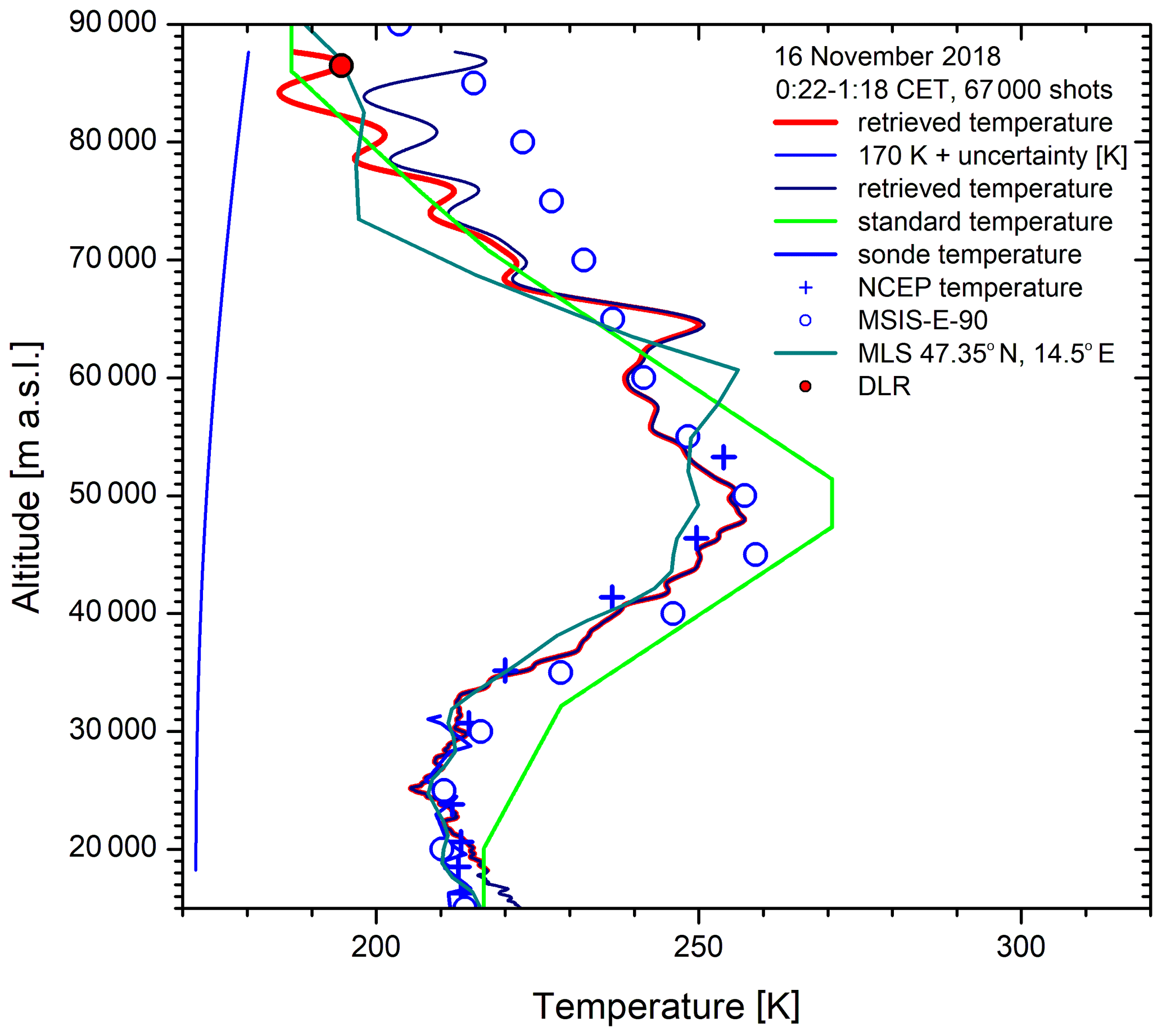
Figure 18 Temperature profile from the measurement in Fig. 21, in comparison with data from the Munich 01:00 CET radiosonde, NCEP (13:00 CET), the MSIS model and MLS; the temperatures were retrieved from the lidar signal by initializing the temperature at about 87 km using both the U.S. Standard and the MSIS values. Both retrievals converge to the same curve within 15–20 km from the top. The red dot shows the temperature from OH airglow measurements at UFS by DLR.

The strong near-field signal peak was attenuated by using a narrow aperture and by rotating the laser beam away from the telescope axis. However, this resulted in a slightly reduced overlap as far as almost 20 km, as can be seen in the temperature data (Fig. 18). The combined raw data were smoothed with a VDI vertical resolution scaling as shown in Fig. 17, the maximum value staying below 2 km.

The temperature data were initialized at 87 $\mathrm{km}\mathrm{a}.\mathrm{s}.\mathrm{l}.$ (density: at 95 km) by using the temperature of the U.S. Standard atmosphere as the starting value. The performance is surprisingly good, despite the strongly growing noise of the raw data in this altitude range. The agreement with the temperatures from the Munich radiosonde and NCEP is very good up to the upper end of the NCEP table (50 km) downloaded from the NDACC website. For higher altitudes, we first compared our results with the MSIS model output calculated for our site, as recommended by Wing et al. (2018). There is a strong discrepancy that could not be reduced by selecting the MSIS temperature at 87 km as the starting value of the retrieval: the temperature converged to the curve for calibrating with the standard atmosphere within just 15 km.

A comparison was made with the temperature of the Microwave Limb Sounder (MLS) during the early hours of 16 November for a position 3.5^∘ farther to the east. Considering the difference in position, the agreement with the MLS temperature profile is quite good, with a strong similarity in structure. The temperature peak at 65 km is present but slightly downward-shifted.

Finally, the mesospheric OH airglow measurements (Schmidt et al., 2013) at UFS by DLR (Deutsches Zentrum für Luft- und Raumfahrt) yielded an average temperature of 194.3 ± 4 K at an estimated 86.5 km during the period of the lidar measurement. This agreement is quite enjoyable. However, there is some uncertainty due to the 45^∘ slant path of the field of view of the OH spectrometer and due to gravity-wave activity indicated in the OH data.

In summary, we are highly satisfied by this first result for a wide-range temperature measurement. In principle, due to the very small average background signal, Poisson effects in the photon statistics must be taken into consideration. More advanced approaches are needed, such as that presented by Sica and Haefele (2015).

8 Discussion and conclusions

The primary goals of the system development described in this paper have been to reduce the measurement time for lower stratospheric water vapour up to at least 20 km to 1 h and to achieve temperature measurements up to more than 80 km. These goals have been met, with a satisfactory performance. Nevertheless, a comparison with the simulations in Sect. 2 clearly shows that the measured lidar signal for water vapour is considerably smaller than predicted.

At 15 km our measurements typically yield H₂O Raman returns of 2 counts per 7.5 m bin and hour. This is converted to 53 counts for the 200 m bins used in the calculation in Sect. 2, one-sixth of the 315 counts simulated. Roughly a factor of 2 is due to the lower laser power in comparison with the 200 W assumed in the simulation. For the rest, apart from uncertainties in the parameters used in the numerical estimate, we found that the most likely reason for this discrepancy is that the Raman cross section used in the calculations is presumably given for the sum of all three ro-vibrational branches. Indeed, the peak signal increased by roughly a factor of 3 when we removed the 347 nm interference filter, which includes the missing attenuation by the interference filter (T = 0.72).

As a consequence, we carried out measurements without an interference filter. However, this resulted in a much higher stratospheric mixing ratio of 120 ppm due to insufficient blocking of 308 or 332 nm radiation. Thus, for collecting the signal from the entire ro-vibrational band, at least a broadband interference filter (bandwidth almost 20 nm) must be added to reject residual contributions from the other channels and to reduce the observed 3 to 4 background counts.

The background is dominated by the size of the entrance slit. The optimum slit width is different for both lasers, given different beam divergences. Therefore, in the future, two additional slits will be used in focal points of the 347 and 355 nm channels (Fig. 8). These slits are more easily accessible than the entrance slit, which facilitates optimization of their position and size.

There are obvious possibilities to enhance the laser power. Better transmitting intra-cavity optics should be installed to significantly reduce the thermal load. A higher transmittance would, therefore, also allow us to remove the cylindrical telescope (Fig. 4) that was introduced to reduce the intra-cavity intensity on the optical components added by us. As a consequence, the resonator would become shorter, and the number of cavity round trips within the fluorescence time of XeCl would grow. As pointed out in Sect. 3.1, the reduction of the numbers of round trips is likely to be the dominant loss factor in the extended resonator.

The calibration of the water-vapour channel was confirmed to be a key issue for the long-term operation of the lidar. We hope that the UFS DIAL can soon be reactivated for this gap to be filled. Additional control by inspecting the data from surrounding radiosonde stations or the signal level at 308 and 332 nm is another important tool to ensure long-term stability of the system. A longer comparison with CFH sensors than in the campaign in February 2019 would also be advantageous. This would be particularly important during periods with fluorescing aerosol in the lower stratosphere in order to assess the influence of this kind of background at 347 nm.

The temperature measurements with a separate, frequency-tripled Nd:YAG laser were quite successful. Improvements could result from using a diode-pumped Nd:YAG laser with a 300 or 350 Hz repetition rate, matching that of the XeCl laser. Such lasers are meanwhile available. We expect lower pulse energies for such a laser at 355 nm, but the 160 mJ currently available yielded too much backscatter signal anyway. The remaining efforts will concentrate on testing the rotational Raman channels with the new spectral filters, on implementing the ozone correction (not possible for the configuration with 353 nm) and on completing the remote control of the lidar system. Automatic control of the alignment is the key to more frequent measurements. Lidar measurements at high temporal resolution may yield more information on the role of atmospheric transport, in particular TST, in the water-vapour concentration in the UTLS. Finally, we are heading for long-term operation of the system with a stable performance in order to provide insight into the H₂O feedback in the climate system.