Estimation of PM_2.5 concentration in China using linear hybrid machine learning model

Satellite remote sensing aerosol optical depth (AOD) and meteorological elements were employed to invert PM_2.5 (the fine particulate matter with a diameter below 2.5 µm) in order to control air pollution more effectively. This paper proposes a restricted gradient-descent linear hybrid machine learning model (RGD-LHMLM) by integrating a random forest (RF), a gradient boosting regression tree (GBRT), and a deep neural network (DNN) to estimate the concentration of PM_2.5 in China in 2019. The research data included Himawari-8 AOD with high spatiotemporal resolution, ERA5 meteorological data, and geographic information. The results showed that, in the hybrid model developed by linear fitting, the DNN accounted for the largest proportion, and the weight coefficient was 0.62. The R² values of RF, GBRT, and DNN were reported as 0.79, 0.81, and 0.8, respectively. Preferably, the generalization ability of the mixed model was better than that of each sub-model, and R² (determination coefficient) reached 0.84, and RMSE (root mean square error) and MAE (mean absolute error) were reported as 12.92 and 8.01 µg m⁻³, respectively. For the RGD-LHMLM, R² was above 0.7 in more than 70 % of the sites and RMSE and MAE were below 20 and 15 µg m⁻³, respectively, in more than 70 % of the sites due to the correlation coefficient having a seasonal difference between the meteorological factor and PM_2.5. Furthermore, the hybrid model performed best in winter (mean R² was 0.84) and worst in summer (mean R² was 0.71). The spatiotemporal distribution characteristics of PM_2.5 in China were then estimated and analyzed. According to the results, there was severe pollution in winter with an average concentration of PM_2.5 being reported as 62.10 µg m⁻³. However, there was only slight pollution in summer with an average concentration of PM_2.5 being reported as 47.39 µg m⁻³. The period from 10:00 to 15:00 LT (Beijing time, UTC+8 every day is the best time for model inversion; at this time the pollution is also high. The findings also indicate that North China and East China are more polluted than other areas, and their average annual concentration of PM_2.5 was reported as 82.68 µg m⁻³. Moreover, there was relatively low pollution in Inner Mongolia, Qinghai, and Tibet, for their average PM_2.5 concentrations were reported below 40 µg m⁻³.

1 Background

In recent years, pollutants have been discharged increasingly in China where air pollution is becoming worse than ever before due to rapid urbanization and industrialization (Wang et al., 2019a). The fine particulate matter (PM_2.5) with a diameter below 2.5 µm is the main component of air pollutants, having considerable impacts on human health, atmospheric visibility, and climate change (Gao et al., 2015; Pan et al., 2018; Pun et al., 2017; Qin et al., 2017). The global concern about PM_2.5 has increased significantly since it was listed as a top carcinogen (Apte et al., 2015; Lim et al., 2020). Currently, ground monitoring is the most efficient method of measuring PM_2.5 (Yang et al., 2018). However, monitoring stations are not evenly distributed due to terrain and construction costs; therefore, it is difficult to obtain a wide range of accurate PM_2.5 concentration data (Han et al., 2015). To solve the problem, the method of estimating PM_2.5 with satellite remote sensing was developed. Satellite remote sensing is characterized by a wide coverage and high resolution (Hoff and Christopher, 2009; Xu et al., 2021). There is also a high correlation between aerosol optical depth (AOD), obtained from satellite remote sensing inversion, and PM_2.5; therefore, AOD is a very effective method of monitoring the spatiotemporal concentration characteristics of PM_2.5.

After Engel-Cox et al. (2004) proposed using satellite AOD to estimate PM_2.5 concentration, several studies have been reported in the literature to address this theory. Based on the regression model, Liu et al. (2005) introduced AOD, boundary layer height, relative humidity, and geographical parameters as the main controlling factors to estimate PM_2.5 in the eastern part of the United States, and the verification coefficient R² obtained was 0.46. Tian and Chen (2010) used AOD, PM_2.5, and meteorological parameters in Southern Ontario, Canada, to establish a semi-empirical model to predict PM_2.5 concentration per hour, and the verification coefficient R² obtained in rural and urban areas was 0.7 and 0.64, respectively. Hu et al. (2013) proposed a geographically weighted regression model to estimate the surface PM_2.5 concentration in southeastern America by combining AOD, meteorological parameters, and land use information. Their model average R² was 0.6. Lee et al. (2012) believed that the satellite remote sensing AOD data would face interference from clouds and snow and ice, and the reliability of the data was questionable. They proposed a mixed model based on AOD calibration to predict the ground PM_2.5 concentration in New England, USA, and achieved good results (R²=0.83). Li et al. (2016) used a PM_2.5 remote sensing method with remote sensing of ground PM_2.5. Combined with MODIS (Moderate Resolution Imaging Spectroradiometer) AOD and ground observation data, Lv et al. (2017) estimated the daily surface PM_2.5 concentration in the Beijing–Tianjin–Hebei region and improved the data resolution to 4 km. Using an interpretable self-adaptive deep neural network, Chen et al. (2021) estimated daily spatially continuous PM_2.5 concentrations across China and analyzed the contribution of various characteristics to the PM_2.5 model. The data used in these early studies are AOD products obtained from polar-orbit satellite sensors. The daily observation frequency is limited. Due to the influence of cloud and ground reflection, the dynamic change information of PM_2.5 cannot be obtained. As a result, geostationary satellite observations can be used to overcome the problem of low temporal resolution for estimating surface PM_2.5 (Emili et al., 2010).

The Himawari-8 satellite commonly used in the Asia-Pacific region is a geostationary satellite launched by the Japan Meteorological Agency in 2014. The observation frequency is 10 min, and the observation results can characterize the aerosols and provide AOD data with a resolution of 5 km (Bessho et al., 2016; Yumimoto et al., 2016). Due to its excellent performance, Wei et al. (2021a) use Himawari-8 data to estimate ground PM_2.5; results show that the CV R² (cross-validation coefficient of determination) is 0.85, with a root mean square error (RMSE) and mean absolute error (MAE) of 13.62 and 8.49 µg m⁻³, respectively. Wang et al. (2017) proposed an improved linear model and introduced AOD, meteorological parameters, and geographic information to estimate PM_2.5 in the Beijing–Tianjin–Hebei region, and the verification coefficient R² was 0.86. T. X. Zhang et al. (2019) used the Himawari-8 hourly AOD product to estimate ground PM_2.5 in China's four major urban agglomerations. The results showed significant diurnal, seasonal, and spatial changes and improved the temporal resolution of estimating PM_2.5 concentration to the hourly level. Yin et al. (2021) used Himawari-8 hourly TOAR (top-of-the-atmosphere reflectance) data to estimate ground PM_2.5 in China, improving the data coverage area.

As research into ground-based PM_2.5 estimation deepens, traditional linear or nonlinear models cannot meet the requirements of large-scale estimation and are gradually being replaced by machine learning algorithms with strong nonlinear fitting abilities (Guo et al., 2021; Mao et al., 2021). Liu et al. (2018) combined Kriging interpolation and a random forest algorithm to obtain the concentration of high-resolution ground PM_2.5 in the United States. To demonstrate the accuracy and superiority of the proposed method, the results were compared with the PM_2.5 concentration in ground measurement stations. Chen et al. (2019) stacked and predicted PM_2.5 concentration based on a variety of machine learning algorithms, discussed the influence of meteorological factors on PM_2.5, and achieved an R² of 0.85. Li et al. (2017a) established a GRNN (generalized regression neural network) model for the whole of China to estimate PM_2.5 concentration, and the results demonstrated that the performance of the deep learning model was better than that of the traditional linear model. In addition, there are some novel algorithms such as the space-time extra-tree (STET) (Wei et al., 2021b) and space-time random forest (STRF) (Wei et al., 2019a) algorithms that are also used for PM_2.5 inversion research.

A large number of existing studies in the broader literature have examined the estimation of ground PM_2.5 concentrations using satellite remote sensing AOD. However, the performance of PM_2.5 estimation models established in the existing studies varies greatly and is not stable in different seasons and regions. To overcome this limitation, in this paper, a restricted gradient-descent linear hybrid machine learning model (RGD-LHMLM) based on a random forest (RF), gradient lifting regression tree (GBRT), and deep neural network (DNN) is proposed to estimate ground PM_2.5 concentration. The model performance is evaluated from time and space to analyze its causes. Finally, spatiotemporal distribution of PM_2.5 concentration in China in 2019 is obtained.

2 Data

2.1 Ground PM_2.5 monitoring data

PM_2.5 concentration data for 2019 used in this study are available from the China National Environmental Monitoring Center (CNEMC) real-time air quality publication system. The PM_2.5 datasets are calibrated and quality-controlled according to national standard GB 3095-2012 (China's National Ambient Air Quality Standards) (China, 2012). The system extracts hourly mean PM_2.5 data. By the end of 2019, China had 1641 monitoring stations built and in operation. Figure 1 shows the spatial distribution of monitoring stations in China.

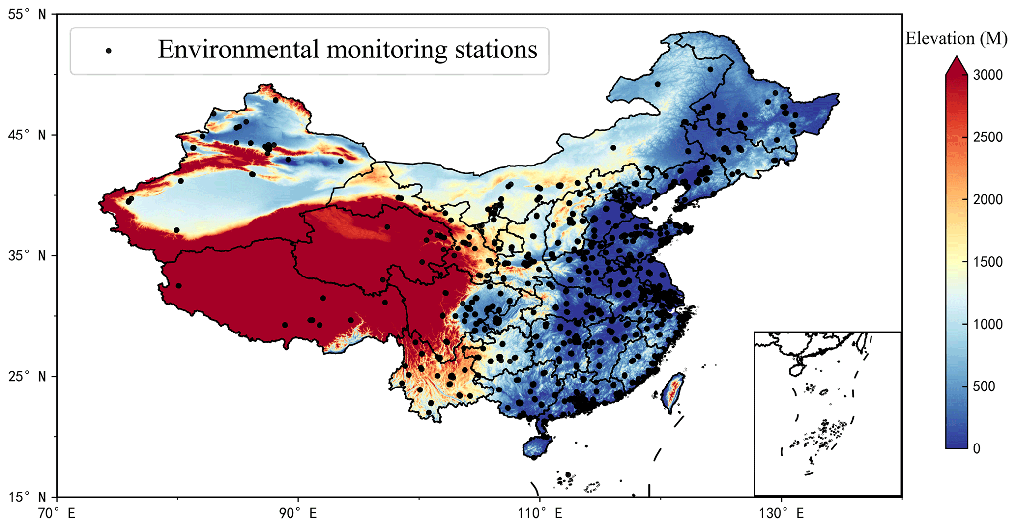
Figure 1 Distribution diagram of environmental monitoring stations in China.

2.2 Satellite AOD data

The Advanced Himawari Imager (AHI) on the Himawari-8 satellite launched by the Japan Meteorological Agency is a highly improved multi-wavelength imager. It adopts the whole disk observation method and has 16 visible and infrared channels. It has the characteristics of fast imaging speed and flexible observation area and time. Himawari-8 AOD is obtained by an aerosol retrieval algorithm based on a Lambertian surface assumption developed by Yoshida et al. (2018). The Level 3 hourly AOD product, released by the Japan Aerospace Exploration Agency (JAXA), provides 500 nm AOD data with a spatial resolution of 5 km during the day. In previous studies (Zang et al., 2018), Himawari-8 AOD was compared with the AOD data of AERONET (Aerosol Robotic Network) in China and achieved good performance (Z. Zhang et al., 2019), so the results show that they are consistent (R²=0.75); RMSE and MAE were 0.39 and 0.21, respectively (Wei et al., 2019b). The AOD data used in this study are the Himawari-8 Level 3 hourly AOD data in 2019 obtained from the Himawari Monitor website of the Japan Meteorological Agency (see “Code and data availability” section). In the study, we selected AOD with strict cloud screening, that is, AOD data with low uncertainty.

2.3 Meteorological data

ERA5 reanalysis data comprise an hourly collection of atmospheric and land-surface meteorological elements that has taken place since 1979 that the European Centre for Medium-Range Weather Forecasts (ECMWF) has used with its prediction model and data assimilation system to reanalyze archived observations (Jiang et al., 2021). Data used in this paper include surface relative humidity (RH, expressed as a percentage), air temperature at a height of 2 m (T_2 m, in K), wind speed (U₁₀, V₁₀; in m s⁻¹), surface pressure (SP, in Pa), boundary layer height (BLH, in m), and cumulative precipitation (RAIN, in m) at 10 m above the ground. A series of studies have indicated that these parameters can affect the concentration of PM_2.5 (Fang et al., 2016; Guo et al., 2017; Li et al., 2017b; Wang et al., 2019b; Zheng et al., 2017; Gui et al., 2019). Uncertainty estimation of ERA5 data has been described in detail on the following website: https://confluence.ecmwf.int/display/CKB/ERA5%3A+uncertainty+estimation (last access: 1 July 2021).

2.4 Auxiliary data

The auxiliary data used in this study include high and low vegetation indices (LH, LL), ground elevation data (DEM), and population density data (PD). The high and low vegetation indices are derived from ERA5 reanalysis data and represent half of the total green leaf area per unit level ground area of high and low vegetation type, respectively. The ground elevation data are derived from SRTM3 (Shuttle Radar Topography Mission, 90 m resolution) measurements jointly conducted by NASA and the US Department of Defense National Imagery and Mapping Agency (NIMA), with a spatial resolution of 90 m. The population data come from the 2015 United Nations GPWv4-Adjusted Population Density data provided by NASA's Socioeconomic Data and Applications Center (SEDAC), which is based on national censuses and adjusted for relative spatial distribution.

3 Method

3.1 Random forest

Random forests (RF) are built based on the combination of a bagging algorithm and decision trees (Breiman, 2001), which are an extended variant of the parallel ensemble learning method (Stafoggia et al., 2019). To construct a large number of decision trees, the random forest model takes multiple samples of the sample data. In the decision trees, the nodes are divided into sub-nodes by using the randomly selected optimal features until all the training samples of the node belong to the same class. Finally, all the decision trees are merged to form the random forest. This method has proved to be effective in regression and classification problems and is one of the best-known machine learning algorithms used in many different fields (Yesilkanat, 2020).

3.2 Gradient-boosted regression trees

Differently from the random forest, gradient boosting regression trees (GBRTs) are based on a boosting algorithm and decision trees (Friedman, 2001). The basic principle of GBRTs is to construct N different basic learners through multiple iterations and constantly add the weight of the learners with a small error probability to eventually generate a strong learner (Johnson et al., 2018). The core of this method is that after each iteration, a learner will be built in the direction of residual reduction (gradient direction) to make the residual decrease in the gradient direction (Schonlau, 2005). The basic learner of the GBRT is the regression tree in the decision tree. During the prediction, a predicted value is calculated according to the model obtained. The minimum square root error is used to select the optimal feature to split the dataset, and the average value of the child node is then taken as the predicted value.

3.3 Deep neural networks

Deep neural networks (DNNs) comprise a supervised learning technique that uses a backpropagation algorithm to minimize the loss function. They adjust the parameters through an optimizer and have high computational power, making them ideal for solving classification and regression problems (Wang and Sun, 2019). The structure of a DNN includes an input layer, an output layer, and several hidden layers. Each layer takes the output of all nodes of the previous layer as the input, and this process requires activation functions. Compared with other activation functions, the linear rectifying function (ReLU) has the advantages of simple derivation, faster convergence, and higher efficiency. At the same time, among the adaptive learning rate optimizers, the AdaMax optimizer performs the best. It not only has the advantages of Adam in determining the learning rate range and having stable parameters in each iteration but also simplifies the method of defining the upper limit range of the learning rate and improves the iteration efficiency (Diederik and Jimmy, 2014). Therefore, in this paper, we selected the AdaMax optimizer and ReLU activation function to train the DNN.

3.4 Model establishment and verification

After data processing, an RF, GBRT, and DNN are used for modeling.

$$\begin{array}{}\text{(1)}& \begin{array}{rl}{\text{PM}}_{\mathrm{2.5}i,j}& ={\text{AOD}}_{i,j}+{\text{BLH}}_{i,j}+{\text{RH}}_{i,j}+{T_{\mathrm{2}\mathrm{m}}}_{i,j}+{\text{LL}}_{i,j}\\ & +{\text{LH}}_{i,j}+{\text{SP}}_{i,j}+{\text{RAIN}}_{i,j}+U_{\mathrm{10}i,j}+V_{\mathrm{10}i,j}\\ & +{\text{PD}}_{i,j}+{\text{HEIGHT}}_{i,j}+{\text{LONG}}_{i,j}+{\text{LAT}}_{i,j}\\ & +{\text{MONTH}}_{i,j}+{\text{HOUR}}_{i,j}\end{array}\end{array}$$

Equation (1) is applicable to the RF, GBRT, and DNN, where PM_2.5i,j is the PM_2.5 at time i at station j.

To prevent model parameters from being controlled by a large or small range of data and speed up the convergence rate of the model, the data must be normalized before starting the training process. Finally, the three optimal sub-models are linearly combined to achieve the final mixed model. To verify the model performance, this paper uses the “10-fold cross-validation” method (Adams et al., 2020). In this method, the data are split into 10 copies, 9 copies for training and 1 copy for verification; this process is repeated 10 times, and then the average of the 10 predictions is computed as the final result. Finally, the predicted value and the measured value are fitted linearly. At the same time, several indicators are used to evaluate the model, including the mean absolute error (MAE; when the predicted value and the true value are exactly equal to 0, that is, the perfect model; the larger the error, the greater the value), the root mean square error (RMSE; when the predicted value and the real value are completely consistent, this is equal to 0, that is, the perfect model; the larger the error, the greater the value), the slope of the fitting equation and the determination coefficient R² (the greater the value, the better the model fitting effect), the bias (Bias; the difference between the predicted values and the true values, so models with larger bias performed worse), and the GEB (generalization error of the bias; it is generally believed that bias should be expressed as a square when using the generalization error). The calculation formula of each indicator is shown as follows:

$$\begin{array}{}\text{(2)}& {\displaystyle }& {\displaystyle }{R}^{\mathrm{2}}=\mathrm{1}-{\displaystyle \frac{{\mathrm{ss}}_{\text{res}}}{{\mathrm{SS}}_{\text{tot}}}},\text{(3)}& {\displaystyle }& {\displaystyle }\text{MAE}={\displaystyle \frac{\mathrm{1}}{n}}{\sum }_{i=\mathrm{1}}^n\left|\widehat{y_i}-y_i\right|,\text{(4)}& {\displaystyle }& {\displaystyle }\text{RMSE}=\sqrt{{\displaystyle \frac{\mathrm{1}}{n}}{\sum }_{i=\mathrm{1}}^n(\widehat{y_i}-y_i{)}^{\mathrm{2}}},\text{(5)}& {\displaystyle }& {\displaystyle }\text{Bias}={\displaystyle \frac{{\sum }_{i=\mathrm{1}}^N\widehat{y_i}-y_i}{N}},\text{(6)}& {\displaystyle }& {\displaystyle }\text{GEB}={\displaystyle \frac{{\sum }_{i=\mathrm{1}}^N(\widehat{y_i}-y_i{)}^{\mathrm{2}}}{N}},\end{array}$$

where $\widehat{y_i}$ represents the predicted value, y_i shows the true value, ss_res denotes the error between the regression data and the mean value, SS_tot represents the error between the real data and the mean value, and the mean value is the mean value of the true value.

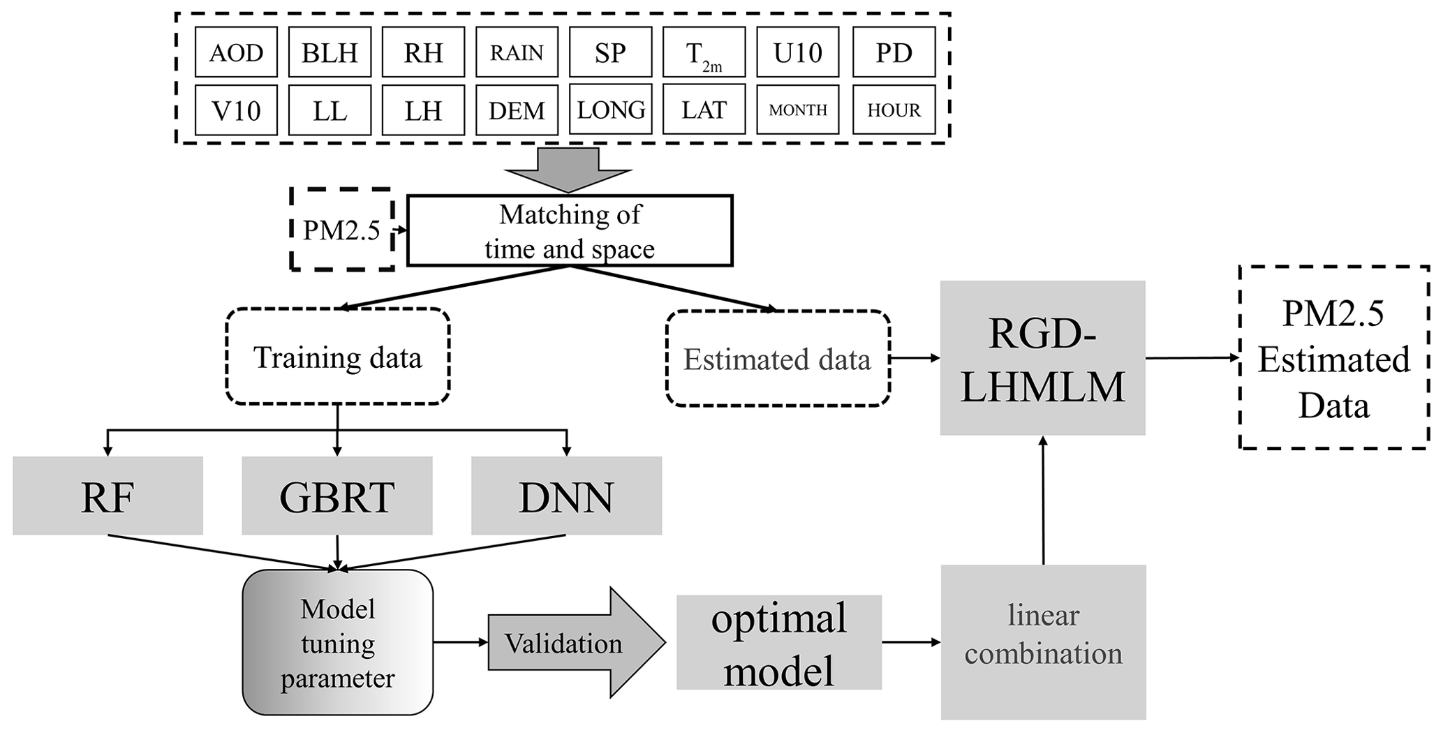
The research process is illustrated in Fig. 2.

Figure 2 Schematic diagram of model.

4 Results and discussion

4.1 Modeling results

According to the above steps, the mixed model RGD-LHMLM is obtained through modeling verification and is compared with the RF, GBRT, and DNN. The fitting and verification accuracy results of each model are shown in Table 1.

Table 1 Comparison of model accuracy.

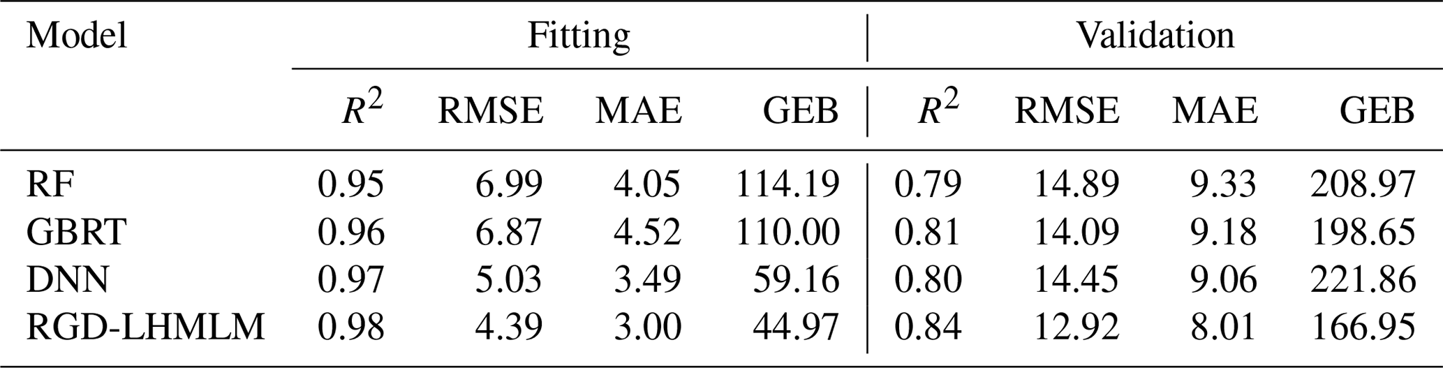
The PM_2.5 inversion results of a single machine learning model show that the DNN has the best inversion performance, followed by the GBRT, and the RF has the worst performance. The expression of the mixing model obtained after linear mixing is as follows:

$$\begin{array}{}\text{(7)}& \begin{array}{rl}{\text{PM}}_{\mathrm{2.5}\text{RGD}-\text{LHMLM}}& =\mathrm{0.25}{\text{PM}}_{\text{2.5RF}}+\mathrm{0.17}{\text{PM}}_{\text{2.5GBRT}}\\ & +\mathrm{0.62}{\text{PM}}_{\text{2.5DNN}}-\mathrm{2.13}.\end{array}\end{array}$$

The weight coefficient of the DNN in the mixed model was the largest (0.62). The R² of RGD-LHMLM in the training set was 0.98, and the RMSE was only 4.39 µg m⁻³, indicating that the model had an excellent data fitting effect. Meanwhile, the generalization ability of the mixed model is also good, with R² of 0.84 and RMSE of 12.92 µg m⁻³ on the validation dataset. Among all the models, the deviation generalization error of the linear mixed model is also the lowest, indicating that the difference between the results obtained by this model and the real value is the lowest. Compared with the RF, GBRT, and DNN, the inversion performance of RGD-LHMLM is improved. In other words, the combination of multiple models can improve the robustness and generalization ability of the model (Wolpert, 1992). The linear fitting equation coefficients between the predicted and measured values in the training set and the verification set were 0.98 and 0.84, respectively, indicating that the prediction accuracy of the model reached a high level. The fitting curve between the model-predicted value and the real value is shown in Fig. 3. The RGD-LHMLM model has the smallest degree of data dispersion, and the slope of the fitting line reaches 0.84, indicating that 84 % of the prediction results are accurate, higher than in the three sub-models. The accuracy of the model decreased in the site-based validation, in which the R² and RMSE values are 0.8 and 14.59 µg m⁻³, respectively.

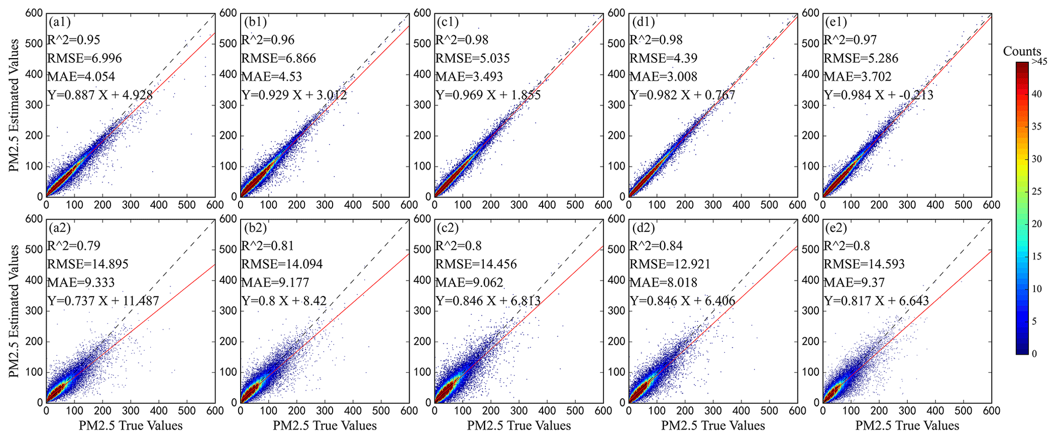
Figure 3 Accuracy of model fitting (the first row) and validation (the second row) (a: RF, b: GBRT, c: DNN, d: RGD-LHMLM (based on sample), e: RGD-LHMLM (based on site)). R² represents the determination coefficient; RMSE represents root mean square error; MAE represents mean absolute error; N represents the number of samples. The equation with terms Y and X represents the fitting relationship between the actual and estimated PM_2.5 values. Dashed black line represents 1:1 line, and red line represents best-fit line from linear regression.​​​​​​​

4.2 Model performance analysis

4.2.1 Bias analysis of model

The average bias of the mixed model in different PM_2.5 concentration ranges was analyzed, and the result is shown in Fig. 4. When the PM_2.5 concentration is less than 60 µg m⁻³, the average bias of the model is less than 0. As the PM_2.5 concentration increases, the model deviation gradually increases. In other words, when the PM_2.5 concentration is small, the predicted value of the model will generally overestimate PM_2.5, and when the PM_2.5 further increases, it will underestimate the PM_2.5 concentration.

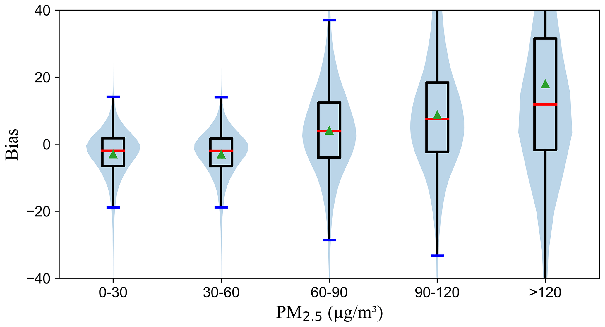
Figure 4 Boxplots of resulting bias (y axis) for different PM_2.5 concentration ranges in µg m⁻³ (x axis) (the green arrow symbol and dark blue and red marks represent the average bias, the median of bias, and the extrema of bias, respectively. Data density is represented by the light blue shading.)

4.2.2 Performance analysis of monitoring station model

The spatial performance of the model was analyzed by measuring R², RMSE, and MAE at the monitoring stations. According to Fig. 5, there are regional differences in the inversion performance of RGD-LHMLM. At all monitoring stations, the average R² was reported as 0.74, and R² was above 0.7 at more than 70 % of the stations, especially in the densely populated and industrially developed areas. The model prediction accuracy was reported as low (R²<0.6) in Xinjiang, Tibet, Qinghai, western Sichuan, and a few other areas of Northeast China. The mean values of RMSE and MAE were reported as 11.4 and 8.01 µg m⁻³, respectively. In fact, the mean values of RMSE and MAE were below 20 and 15 µg m⁻³ in more than 95 % of stations, showing a low estimation error.

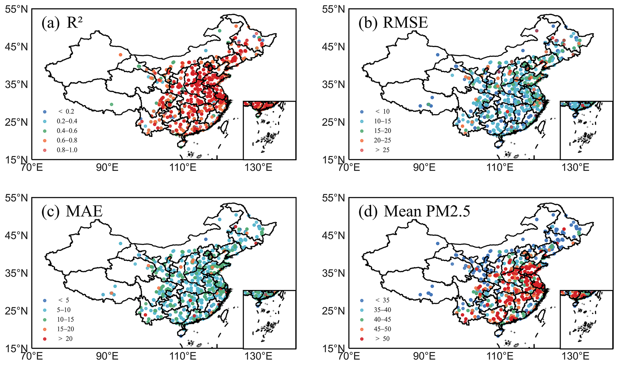
Figure 5 Spatial distributions of model precision in terms of (a) determination coefficient (R²), (b) root mean square error (RMSE), (c) mean absolute error (MAE), and (d) mean PM_2.5 concentration at each site in China. Colored circles represent different value ranges of statistical parameters shown.

Based on the analysis of spatial differences in the RGD-LHMLM inversion performance, the following deductions can be made. First, the environmental monitoring stations in the central and eastern regions with better inversion performance were distributed densely, and there are many data available; therefore, the model had a satisfactory training effect. Moreover, data matching was lower in the western region than in other regions, something which resulted in model over-fitting and reduced accuracy (Zhang et al., 2018). Second, some areas of western and northeastern China are covered by snow and the Gobi Desert has high surface albedo. This reduces the accuracy of AOD obtained by satellite observation and introduces errors into model training. Finally, the Himawari-8 scanning range is limited, and the satellite observation data obtained in western China are limited in terms of quantity and accuracy. In general, RGD-LHMLM has a satisfactory spatial performance, especially in areas with high annual average concentrations of PM_2.5; therefore, it can have a good inversion effect.

4.2.3 Timescale model performance analysis

Figure 6 shows the scatterplot fitted with the inversion results of the mixed model from 9:00–17:00 LT. The model R² ranged from 0.556 to 0.88 at different times. Except for 17:00 LT when the model had the worst performance, the model R² exceeded 0.7, indicating that the model had a good performance. The optimal performance time is 13:00 LT when R² is 0.88. According to the results, the hourly differences in model performance were significant.

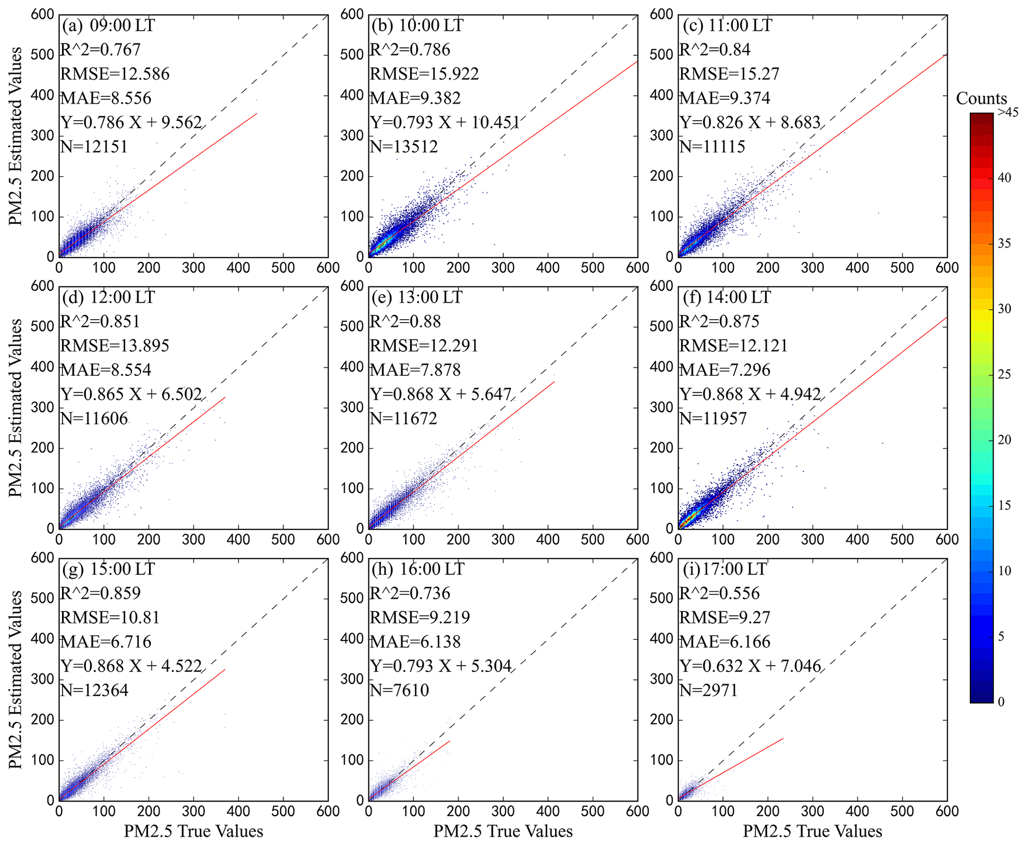
Figure 6 Density scatterplot of actual hourly PM_2.5 values (x axis) and model-estimated values (y axis) in hourly PM_2.5 estimates in China from (a) 09:00 LT to (i) 17:00 LT. R² represents the determination coefficient; RMSE represents root mean square error; MAE represents mean absolute error; N represents the number of samples. The equation with terms Y and X represents the fitting relationship between the actual and estimated PM_2.5 values. Dashed black line represents 1:1 line, and red line represents best-fit line from linear regression.

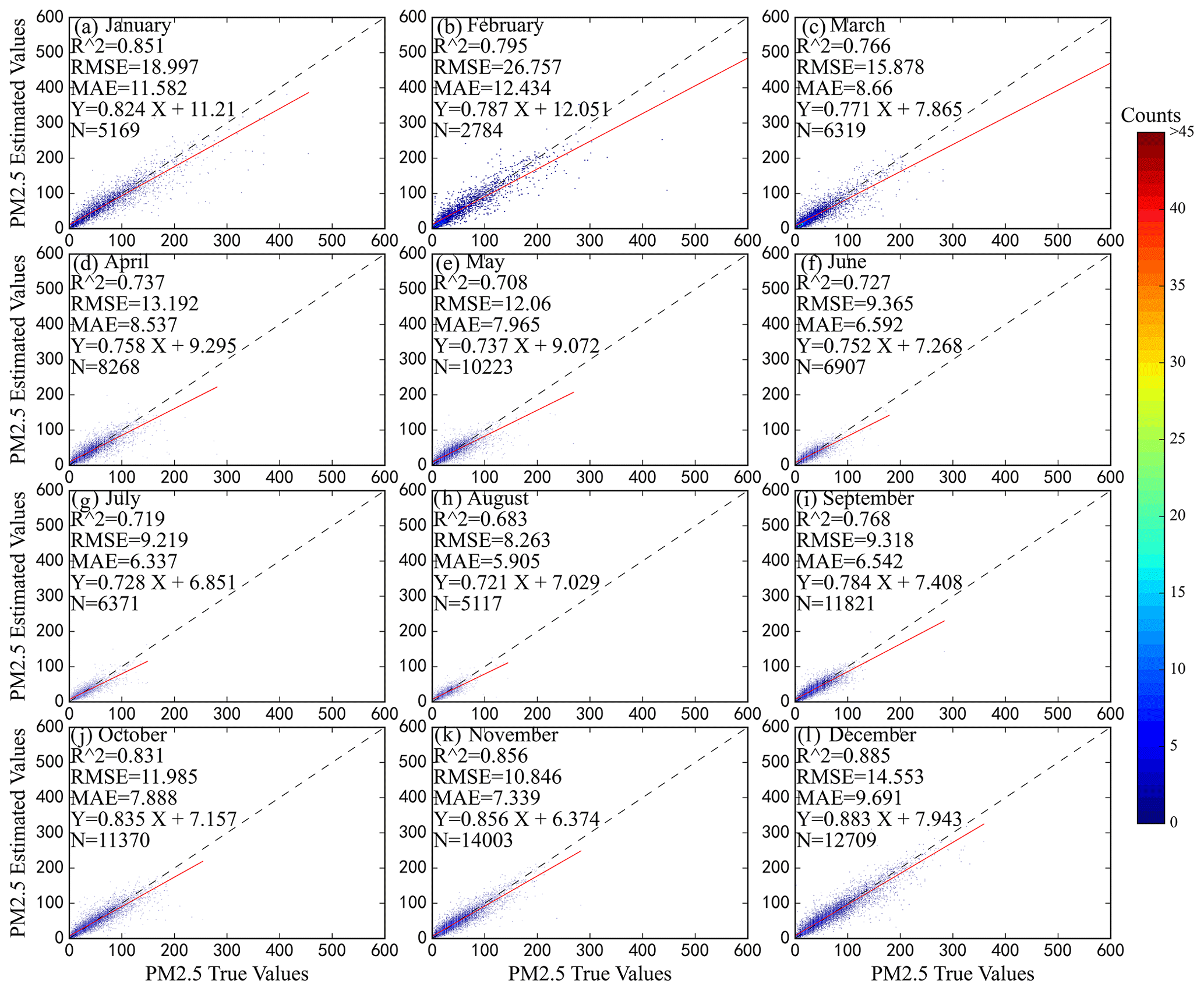
Figure 7 shows the inversion performance results of the hybrid model collected from January to December 2019. The model performed the worst in the summer months – June, July, and August – when R² was reported as 0.73, 0.72, and 0.68, respectively; however, RMSE and MAE were only 9.37, 9.22, 8.26 and 6.59, 6.34, and 5.91 µg m⁻³, respectively, due to the lower average concentration of PM_2.5 in summer. Winter and autumn models gained better performance results with an average R² over 0.8. However, in contrast to those of summer, the estimation errors of these two seasons were relatively large, with average RMSE of 20.10 and 10.72 µg m⁻³ and average MAE of 11.20 and 7.25 µg m⁻³, respectively. The mean R² was 0.74, and the mean RMSE and MAE were 13.71 and 8.39 µg m⁻³, respectively.

Figure 7 Same as Fig. 6 but for monthly PM_2.5 estimates.

4.2.4 Feature importance analysis

The model performance differences were also analyzed to extract and rank the model features of the RF and GBRT based on the feature importance. The higher the feature importance, the greater the contribution of factors to the model. Figure 8 shows that AOD, boundary layer height, 2 m surface temperature, and relative humidity had the greatest effect on the mixed model performance out of all variable characteristic parameters. Accordingly, AOD is greatly affected by the fine particulate matter and is the main factor in the inversion of PM_2.5. Changes in the boundary layer height can affect the diffusion ability of the atmosphere. If the boundary layer height is low, the accumulation of pollutants will be caused. At the same time, the 2 m surface temperature has a great impact on the boundary layer height (Miao et al., 2018). Finally, higher rates of atmospheric humidity can improve the fine particulate matter accumulation.

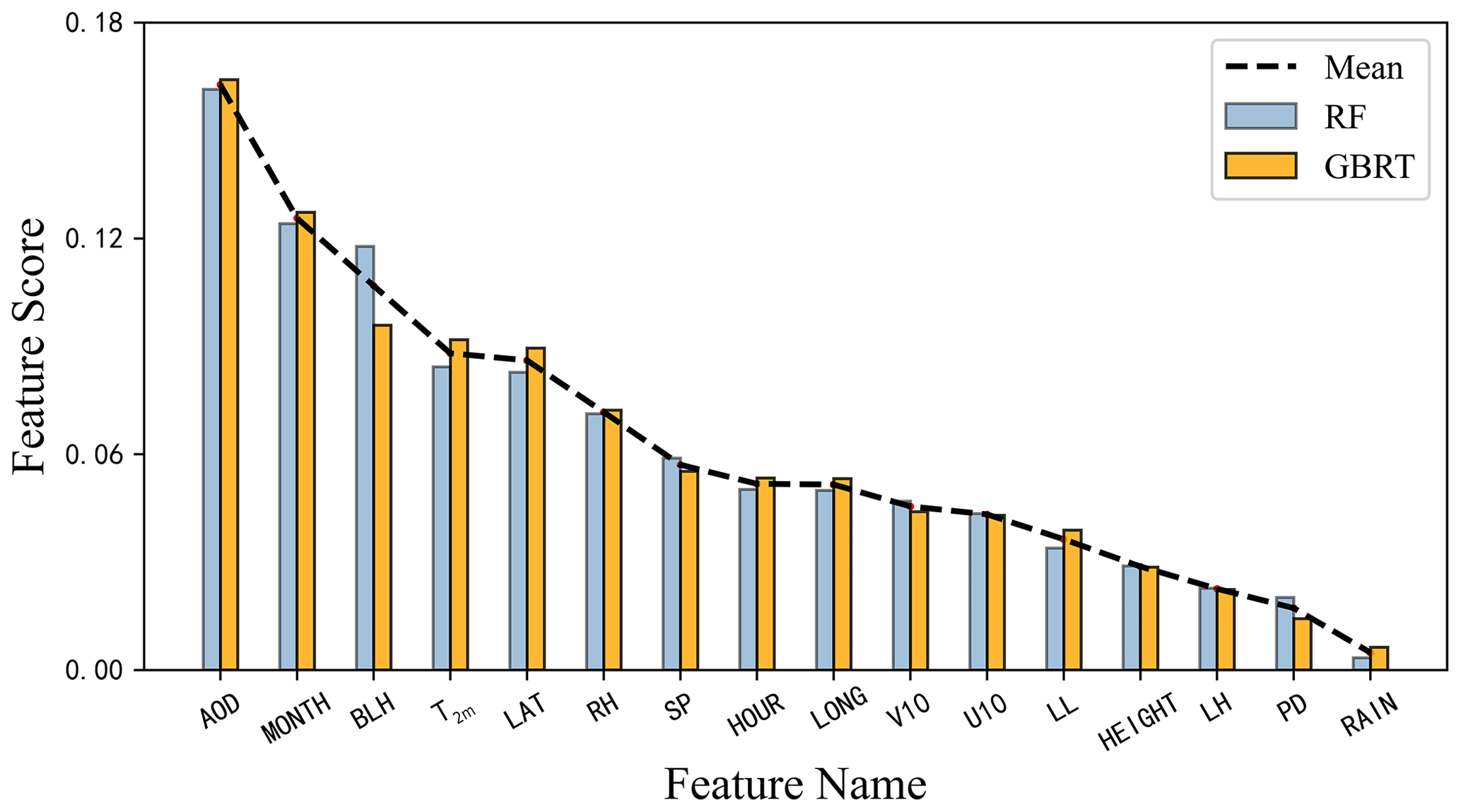
Figure 8 Score (y axis) for each model contributing feature factor (x axis) for the RF (blue) and GBRT (orange). Dashed line represents the mean values.

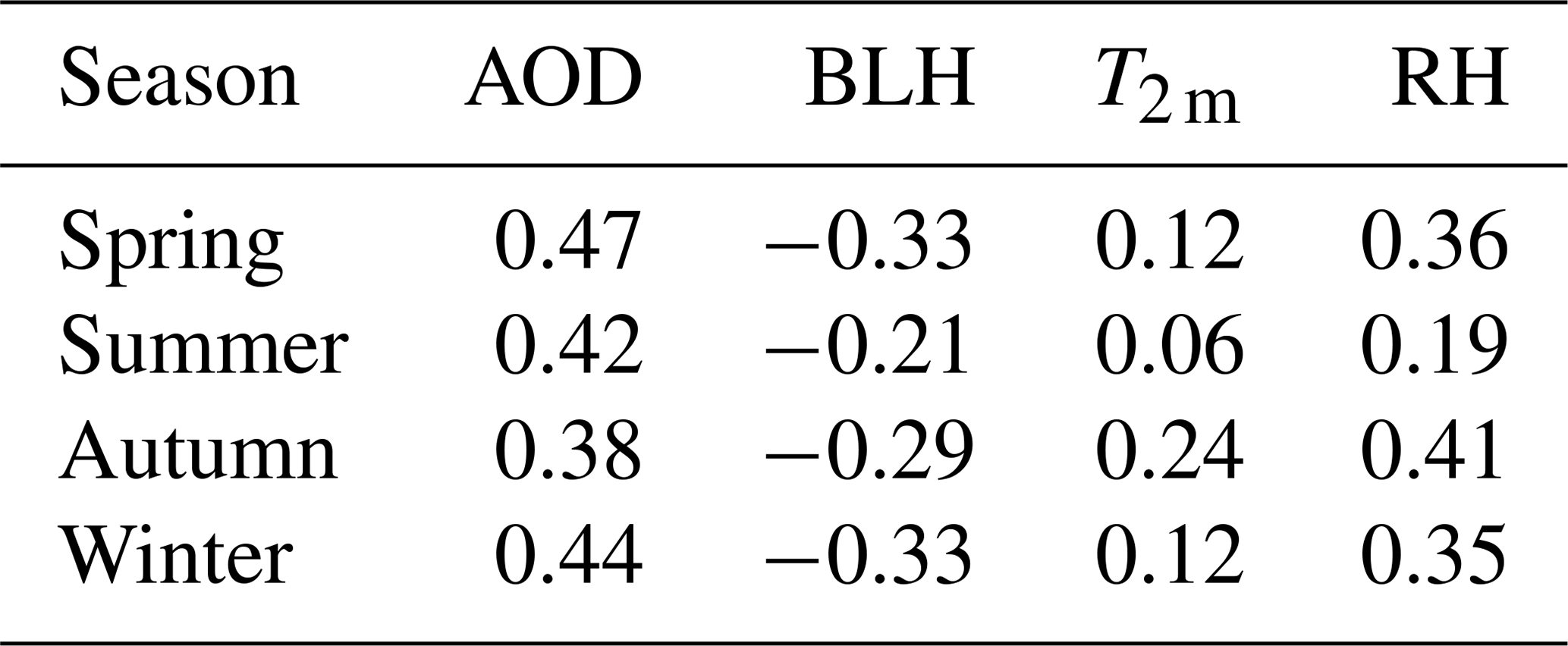
As shown in Fig. 9, the correlation coefficients between the monthly mean values of important meteorological parameters (AOD, BLH, T_2 m, and RH) and R² were also analyzed. According to the results of Table 2, the correlation coefficients between the meteorological parameters and PM_2.5 were lower in summer. Furthermore, there are many rainy days and large cloud coverage, which is not conducive to satellite observation and decreases the accuracy of AOD data in summer. Therefore, the summer model performance is poor. There was a strong correlation between meteorological parameters and PM_2.5 in autumn. There were also similar correlations between spring and winter; however, the winter model performed better. The reasons can be interpreted as follows. The winter temperature and boundary layer height are low, whereas the atmosphere is stable but not conducive to the diffusion of pollutants. Moreover, during the heating period in winter, pollutant emissions soar greatly and result in a sharp rise in the concentration of PM_2.5. The increased pollution in winter ensures the quality and quantity of data, thereby improving the model performance effectively.

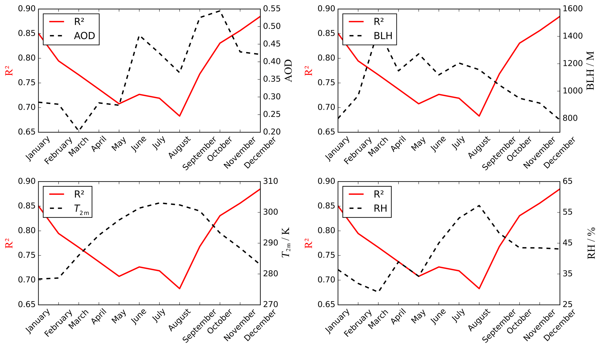
Figure 9 Annual variability (x axis) in monthly average of meteorological parameters AOD, BLH (m), T_2 m (K), and RH (%) (right y axis) and R² (left y axis).

Table 2 Correlation coefficient between meteorological parameters with PM_2.5.

4.3 Temporal and spatial distribution characteristics of PM_2.5 concentration in China

In terms of spatial distribution, Shandong, Henan, Jiangsu, and Anhui, as well as parts of Hubei and Hebei, were the most polluted areas in China in 2019, with an annual average PM_2.5 concentration of 82.86 µg m⁻³. On the one hand, these areas are economically developed and densely populated, resulting in a large quantity of pollutant emissions. On the other hand, the barrier of the peripheral mountains (Taihang Mountains, the Qinling, and the southern hills) leads to the accumulation of pollutants that are difficult to diffuse. The Sichuan Basin is a rare area with a high PM_2.5 value due to its unique topography (L. Zhang et al., 2019), with an annual average PM_2.5 concentration of 64.69 µg m⁻³. In addition, in Inner Mongolia, Qinghai, Tibet, and other places, the pollution level is low: the average annual PM_2.5 concentration is less than 40 µg m⁻³.

The temporal distribution of PM_2.5 is shown in Fig. 10, The PM_2.5 concentration began to rise from 09:00 LT, and peaked at 55.65 µg m⁻³ between 10:00 and 11:00 LT every day. After that, it maintained a high concentration until 15:00 LT and then began to decrease. In the most polluted areas of China, the peak concentration of PM_2.5 can reach 85.05 µg m⁻³, while the peak in the less polluted areas is only about 40 µg m⁻³. On a national scale, daily PM_2.5 concentrations fluctuate slightly.

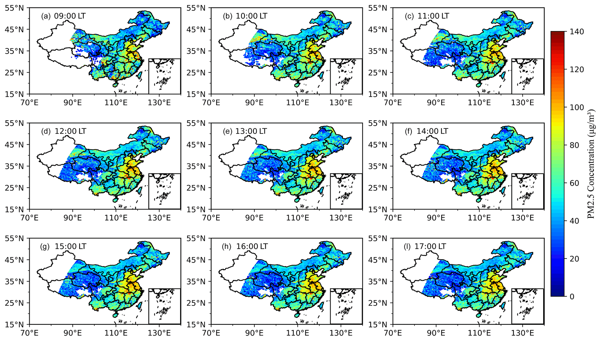
Figure 10 Hourly spatial distribution of PM_2.5 concentration in China at different local times from (a) 09:00 LT to (i) 17:00 LT.

PM_2.5 concentration in China varies significantly with the seasons. As shown in Fig. 11, PM_2.5 concentration in winter is the highest, with an average value of 62.10 µg m⁻³. January 2019 was the most polluted month in China, with the average PM_2.5 concentration reaching 63.58 µg m⁻³. The average PM_2.5 concentration was 47.39 µg m⁻³ in summer. The average concentration of PM_2.5 in spring and autumn was 54.21 and 52.26 µg m⁻³, respectively, indicating similar levels of pollution.

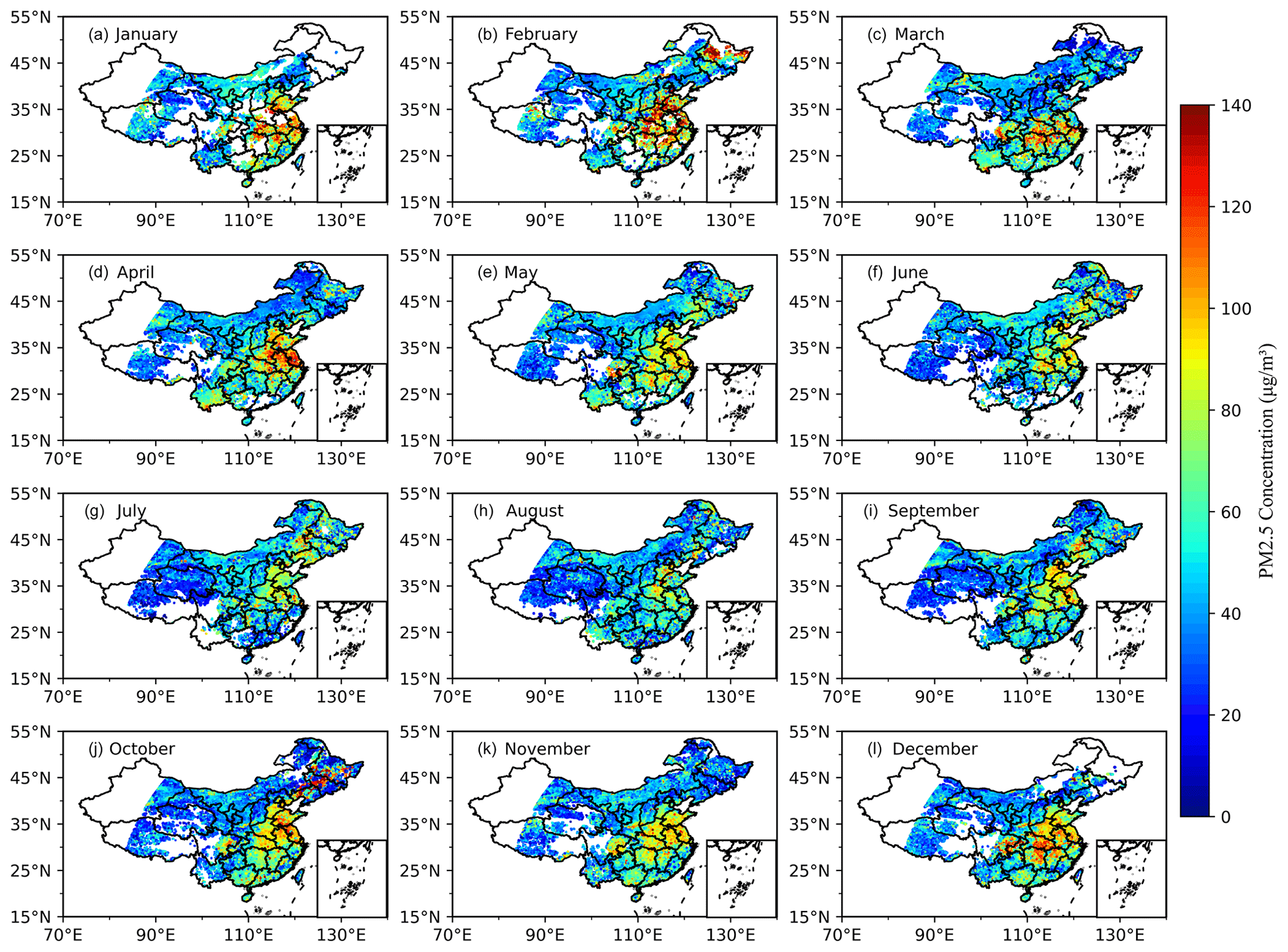
Figure 11 Same as Fig. 10 but for monthly spatial distribution.

5 Conclusions

It is essential to collect the spatiotemporal evolution characteristics regarding the concentration of PM_2.5 for air pollution prevention and containment. Based on the linear hybrid machine learning model, this paper used the AOD data of Himawari-8 to invert the concentration of PM_2.5 in China and obtain its distribution characteristics. The model performance and inversion results are analyzed and summarized below:

1. In the RGD-LHMLM obtained from linear fitting, the DNN accounted for the largest proportion with a weight coefficient of 0.62. The R² of RGD-LHMLM was 0.84, and its generalization ability was significantly better than that of a single model (DNN, 0.80; GBRT, 0.81; RF, 0.79). Moreover, RMSE and MAE were 12.92 and 8.01 µg m⁻³, respectively.

2. RGD-LHMLM was spatially stable, with R²>0.7 in more than 70 % of sites as well as RMSE < 20 µg m⁻³ and MAE < 15 µg m⁻³ in more than 95 % of sites. These sites are mainly located in densely populated and industrially developed areas. The correlation difference between the inversion factor and PM_2.5 in various seasons would lead to seasonal variations in the model performance. In addition, the performance was the worst in summer with an average R² of 0.71; winter showed the best performance with an average R² of 0.84. The diurnal variation in the model inversion effect is also obvious, and the 11:00–14:00 LT model usually has better performance.

3. Changes in the spatiotemporal characteristics were obvious in the concentration of PM_2.5 in China. In other words, North China and East China had the highest concentration of PM_2.5 with an average annual concentration of 82.86 µg m⁻³, whereas Inner Mongolia, Qinghai, Tibet, and other regions had low pollution levels with an average annual concentration of PM_2.5 below 40 µg m⁻³. In winter, the concentration of PM_2.5 was higher with an average of 62.10 µg m⁻³, whereas the pollution was lighter in summer with an average concentration of PM_2.5 being reported 47.39 µg m⁻³. In the most polluted areas, the peak concentration of PM_2.5 could reach 85.05 µg m⁻³, but the daily PM_2.5 concentration fluctuated slightly.

In conclusion, RGD-LHMLM can accurately measure the concentration of PM_2.5 and demonstrate the seasonal evolution of pollutants. These results can help control the local pollution. This study also indicated that integrating multiple machine learning models improved the accuracy of fitting results effectively. For more accurate pollutant data, such models can be employed to fit the PM_2.5 in the future with more parameters closely related to PM_2.5. However, there are some vacant values in the results of this study. There are also no data for some areas. Thus, other satellite data can be used in future studies to solve this problem.