Measurements of CFC-11, CFC-12, and HCFC-22 total columns in the atmosphere at the St. Petersburg site in 2009–2019

Monitoring atmospheric anthropogenic halocarbons plays an important role in tracking their atmospheric concentrations in accordance with international agreements on emissions of ozone-depleting substances and, thus, in estimating the ozone layer recovery.

Within the Network for the Detection of Atmospheric Composition Change (NDACC), regular Fourier transform infrared (FTIR) measurements can provide information on the abundancies of halocarbons on a global scale. We improved retrieval strategies for deriving the CFC-11 (CCl₃F), CFC-12 (CCl₂F₂), and HCFC-22 (CHClF₂) atmospheric columns from IR solar radiation spectra measured by the Bruker IFS125HR spectrometer at the St. Petersburg site (Russia). We used the Tikhonov–Phillips regularization approach for solving the inverse problem with optimized values of regularization parameters. We tested the strategies developed by comparison of the FTIR measurements with independent data. The analysis of the time series of column-averaged dry air mole fractions (Xgas) measured in 2009–2019 gives mean values of 225 pptv (parts per trillion by volume; CFC-11), 493 pptv (CFC-12), and 238 pptv (HCFC-22). Trend values total −0.40 % yr⁻¹ (CFC-11), −0.49 % yr⁻¹ (CFC-12), and 2.12 % yr⁻¹ (HCFC-22).

We compared the means, trends, and seasonal variability in X_CFC-11, X_CFC-12, and X_HCFC-22 to that of (1) near-ground volume mixing ratios (VMRs), measured at the observational site Mace Head, Ireland (GVMR), (2) the mean in the 8–12 km layer VMRs, measured by ACE-FTS and averaged over 55–65^∘ N latitudes (SVMR), and (3) Xgas values of the Whole Atmosphere Community Climate Model (WACCM) for the St. Petersburg site (WXgas).

In general, the comparison of Xgas with the independent data showed a good agreement of their means within the systematic errors of the measurements considered. The trends observed over the St. Petersburg site demonstrate the smaller decrease rates for X_CFC-11 and X_CFC-12 than that of the independent data and the same increase rate for X_HCFC-22. As a whole, Xgas, SVMR, and WXgas showed qualitatively similar seasonal variations, while the GVMR variability is significantly less, and only the WX_HCFC-22 variations are essentially smaller than that of X_HCFC-22 and SVMR_HCFC-22.

1 Introduction

Since the middle of the 20th century, anthropogenic trace gases, the molecules of which contain halogens, due to their specific physical and chemical properties, have been actively used in the climatic and refrigeration industry, as well as in various propellants. Molina and Rowland (1974) have shown that these gases play an important role in the destruction of stratospheric ozone. In particular, the photolysis of CCl₃F (trichlorofluoromethane; CFC-11) and CCl₂F₂ (dichlorodifluoromethane; CFC-12) in the stratosphere leads to the appearance of active chlorine, which is involved in ozone depletion reactions. The WMO (2018, Appendix A) estimates the ozone depletion potential (ODP) of CFC-12 as being 0.73–0.81 (the ODP of CFC-11, chosen as a reference, equals 1). Although the major content of these gases is concentrated in the troposphere, in the equatorial region, the global circulation moves them out into the lower and middle stratosphere and transports them to high-latitude regions. In the stratosphere, chlorofluorocarbons (CFCs) are photochemically decomposed to chlorinated free radicals (Cl and ClO) that are deactivated into chlorine reservoirs of HCl, ClONO₂, and HOCl (WMO, 1985, Chapter 3). In polar regions, heterogeneous reactions on the surfaces of polar stratospheric clouds and cold sulfate aerosols convert inert reservoir molecules into active forms that photolyze, producing free radicals, and cause the chemical ozone depletion in spring through catalytic cycles resulting up to the appearance of ozone holes (Solomon et al., 2014).

As the result of the Montreal Protocol and its amendments and adjustments that restricted the production of CFCs (see WMO, 2018), the industry moved away from CFCs to less ozone-depleting hydrochlorofluorocarbons (HCFCs), especially CHClF₂ (chlorodifluoromethane; HCFC-22). Although the ODP of HCFC-22 is much lower than that of CFCs, it is an ozone-depleting substance too. Ozone depletion by HCFC-22 is primarily associated with the heating of the stratosphere, and its ODP, although small, totals 0.024–0.34.

CFC-11 and CFC-12, like HCFC-22, also absorb infrared radiation; therefore, they are all greenhouse gases. The global warming potential (GWP) represents the integrated radiative forcing (RF) for a conditional time horizon (20, 100, and 500 years) caused by emissions of a unit mass of a gas relative to the same RF value of CO₂ that is chosen as a reference for estimating the GWP of other gases. According to WMO (2018, Appendix A), the GWP for 100 years is 5160 for CFC-11, 10 300 for CFC-12, and 1780 for HCFC-22. One of the reasons for the high GWP values of these gases is their long lifetimes, i.e., 52, 102, and 11.9 years, respectively. Due to their long lifetimes, these gases are also good indicators for studying the transport and mixing processes in the upper troposphere and the lower stratosphere (e.g., Hoffmann and Riese, 2004).

After Molina and Rowland (1974) reported that the CFCs accumulating in the Earth's atmosphere led to an increased rate of ozone depletion, the attention of both scientists and policymakers to the ozone hole problem increased. Nowadays, monitoring of ozone and other stratospheric gases, as well as ozone-depleting substances, including CFCs, is crucial for testing the theories of the ozone hole formation mechanism (Cracknell and Varotsos, 2009).

The Montreal Protocol from 1987, which came into force in 1989, limited the production and consumption of CFCs. Later on, in 1992, in Copenhagen, and in 1995, in Vienna, the phasing out of CFCs was started by the end of 1995 in developed countries and by the end of 2010 in developing countries. Therefore, the atmospheric burden of CFC-11 and CFC-12 was declining at an average rate of 0.7 % yr⁻¹–1.2 % yr⁻¹ and 0.4 % yr⁻¹–0.5 % yr⁻¹, respectively (Brown et al., 2011). ACE-FTS (Atmospheric Chemistry Experiment and Fourier transform spectrometer) satellite measurements in the last 16 years (Bernath et al., 2020a) have illustrated the success of the Montreal Protocol by demonstrating decreasing trends in CFC-11 (−0.53 % yr⁻¹) and CFC-12 (−0.61 % yr⁻¹) abundancies and a slowing rate of increase in HCFC-22 abundancies (1.8 % yr⁻¹). ACE-FTS estimates are made for latitudes between 60^∘ S and 60^∘ N and for altitudes between 5.5 and 10.5 km. Nevertheless, with its accumulation in the troposphere, CFC-11 still provides a quarter of all chlorine reaching the stratosphere. The time needed for recovery of the ozone layer depends, among other factors, on the sustainability of the reduction in the atmospheric concentrations of CFC-11, CFC-12, and other halocarbons.

Based on the 2015–2017 data, Montzka et al. (2018) showed that the rate of change in the CFC-11 atmospheric concentrations decreased by approximately half to −0.4 % yr⁻¹, assuming that this slowdown is caused by the emergence of new, unregistered sources. This finding enhances the importance of the CFC-11 monitoring. The maximum of the CFC-12 atmospheric concentrations was observed in the early 2000s; since then, its steady decrease has been detected with an average rate of 0.4 % yr⁻¹ to 0.5 % yr⁻¹ (Advanced Global Atmospheric Gases Experiment (AGAGE) network; http://agage.mit.edu/data/agage-data, last access: 3 August 2020). As HCFCs are “transitional substances” for the replacement of CFCs, their production has increased rapidly in developed countries in the 1990s and peaked in the mid-1990s. Under the Montreal Amendment (1997), all countries must gradually phase down HCFCs. In September 2007, it was decided to accelerate the phasing out of HCFCs. Developed countries were reducing their consumption of HCFCs and completely phased them out by 2020. Developing countries agreed to start their phase-out process in 2013 and are now following a stepwise reduction until the complete phase out of HCFCs by 2030.

On a global scale, two data sources are mainly used to study the trends and seasonal variations in the target gases, i.e., local measurements of near-ground concentrations (e.g., the AGAGE networks, Dunse et al., 2005, NOAA's Halocarbons & other Atmospheric Trace Species (HATS) and Chlorofluorocarbon Alternatives Monitoring Project (CAMP), Montzka et al., 1993), and satellite limb measurements by the Improved Limb Atmospheric Spectrometer (ILAS), ACE-FTS, and Michelson Interferometer for Passive Atmospheric Sounding (MIPAS; Hoffmann et al., 2008; Mahieu et al., 2008; Eckert et al., 2016; Kellmann et al., 2012; Boone et al., 2020). In contrast to satellite and in situ measurements near ground, ground-based Fourier transform infrared (FTIR) measurements of solar radiation are sensitive to changes in total columns (TCs) of atmospheric gases. The FTIR method complements the information obtained by the first two methods, although it does not allow detailed information on the vertical gas distribution to be retrieved.

The first FTIR measurements of atmospheric HCFC-22 were performed from the balloon in early 1980s (Goldman et al., 1981). Later, with the appearance of high-resolution instruments, halocarbons started to be derived with ground-based FTIR spectrometers. In the last few decades, TCs of halocarbons are more actively measured by ground-based FTIR methods (e.g., Notholt, 1994; Rinsland et al., 2005, 2010; Zander et al., 2005; Mahieu et al., 2010, 2013, 2017; Zhou et al., 2016; Prignon et al., 2019). Time series of CFC-11, CFC-12, and HCFC-22 TCs above the Jungfraujoch station, Switzerland, are presented in World Meteorological Organization (WMO) reports on the scientific assessment of ozone depletion (e.g., WMO, 2018).

Within the Network for the Detection of Atmospheric Composition Change (NDACC; http://www.ndaccdemo.org/, last access: 28 July 2021), regular FTIR measurements provide information on TCs of a number of atmospheric trace gases, including halocarbons, with a large spatial coverage (at 19 out of 77 network stations located at latitudes between 78^∘ S and 80^∘ N). Mahieu et al. (2017) reported on the results of R-142b measurements, along with the comparison with independent data and the trend estimates. Zhou et al. (2016) showed the results of CFC-11, CFC-12, and HCFC-22 measurements at two NDACC sites on Réunion island for the period of 2004–2016, including the trend estimates and the comparison with the satellite data. Prignon et al. (2019) proposed a technique for estimating two partial columns and TCs of HCFC-22 at the Jungfraujoch mountain station and a corresponding time series of HCFC-22 TCs for 1988–2017, along with a trend analysis for various time periods.

The archive of ground-based spectroscopic measurements of IR solar radiation, performed at the NDACC site of St. Petersburg (Timofeyev et al., 2016; Virolainen et al., 2017) since 2009, has been used to derive TCs of CFC-11, CFC-12, and HCFC-22. First, in Russia, estimates of CFC-11 TCs using the FTIR method and the original retrieval technique were given by Yagovkina et al. (2011). Polyakov et al. (2018) presented the preliminary results of CFC-11, CFC-12, and HCFC-22 TCs retrieval for the period of 2009–2016, using the SFIT4 software (version 0.9.4.4) described by Hase et al. (2004). It should be noted that the SFIT4 software is a versatile tool, and it is necessary to customize it for a specific task through the selection and tuning of numerous parameters. Polyakov et al. (2018) selected these parameters, based on the studies at other NDACC sites (Mahieu et al., 2010; Zhou et al., 2016), and the general recommendations of the IR working group (IRWG) of the NDACC network. However, these first results raised a several problems; in particular, there was an unreasonably large scatter of the TC values and significant seasonal variations. A later study showed that the scatter and seasonal variability observed were not due to objective reasons but due to peculiarities in the processing retrieval technique.

The information content of the FTIR spectra, with respect to target gases abundancies, is not large, due to several reasons. First, the absorption of CFC-11 and HCFC-22 is not strong. Even for a solar elevation of about 15^∘, the transmission of solar radiation caused by CFC-11 absorption is greater than 90 %, and for HCFC-22, it is close to 75 %. For a solar elevation of about 50^∘, these values are estimated as being 96 % and 95 %, respectively. Second, there is the absorption of interfering gases in the spectral range considered. Thus, the CFC-11 absorption band overlaps with several strong water vapor absorption lines and the HNO₃ absorption band, and each of the CFC-12 and HCFC-22 absorption bands overlap a wing of the water vapor absorption line (see Appendix A). Finally, the CFC-12 and, to a larger extent, the CFC-11 bands have a smoothed spectral dependency of absorption that requires the use of wide microwindows for retrieving their abundancies, i.e., 2 cm⁻¹ for CFC-12 and not smaller than 30 cm⁻¹ for CFC-11. These factors cause difficulties in halocarbon retrieval from FTIR spectra measurements.

Later, the retrieval techniques for estimating CFC-11, CFC-12, and HCFC-22 TCs by the FTIR method at the St. Petersburg site were refined and improved. These techniques were described in detail by Polyakov et al. (2019a, b, 2020b). In the current study, we present the main features of the techniques developed and analyzed using the Tikhonov–Phillips (T−Ph) approach. The time series of CFC-11, CFC-12, and HCFC-22 TCs were extended until the fall of 2019. The time series of the TCs were analyzed and compared to independent measurements and numerical modeling data.

2 Technique for inverting the spectroscopic measurements

2.1 Spectroscopic measurements

The main features of the ground-based station, observational system, and the technique for measuring the solar spectra used in this study were described in detail by Timofeyev et al. (2016).

The St. Petersburg site is located in Peterhof, 30 km west of the city of St. Petersburg. The latitude of the site (59.88^∘ N) predetermines winter measurements with a low solar elevation; in December–January, the maximal solar elevation does not usually exceed 20^∘, and spectroscopic measurements are performed up to a solar elevation of 5^∘. Due to peculiarities of the local weather, measurements are mainly (76 %) carried out in the spring and summer seasons. The spectra analyzed are obtained without any additional apodization of the interferograms, and their spectral resolution is 0.005 cm⁻¹. The observational system is based on a Bruker IFS125HR Fourier spectrometer, but some of the equipment is nonstandard. Before February 2016, a nonstandard (for the IRWG-NDACC sites) spectral filter (hereinafter F3) was used for measurements in a spectral region with the absorption bands of the target gases. Since this filter was plane-parallel, a parasitic interference arose in it, leading to the appearance of an effect of the optical resonance Blumenstock et al. (“channeling”; see 2020). In addition, a homemade solar tracking system is used.

The period of channeling is caused by the material and the thickness of the filter, and in the spectral region (800–900 cm⁻¹), it is close to 1.1 cm⁻¹, while the channeling amplitude varies from zero to a few percent, depending randomly on the filter positioning. To analyze the presence and the channeling amplitude, we performed the Fourier analysis in the most transparent spectral range (892–905 cm⁻¹) for harmonic components, with interval periods of 1–1.25 cm⁻¹. The channeling amplitude was calculated relative to the mean signal value in this spectral range.

The SFIT4 software supports the accounting for channeling, and its compensation is in a spectrum. Before September 2009, some of the spectra measured had significant values of the channeling amplitude. We excluded spectra with a channeling amplitude that exceeds 2 % from further processing, assuming that such a distortion of the spectra is too great. Afterwards, the filter was installed so as to minimize channeling. In addition, we analyzed the autocorrelation coefficient of a dark noise in the range of 660–680 cm⁻¹ (except for a slope) and excluded the spectra with an averaged autocorrelation coefficient greater than 0.1. A large autocorrelation coefficient of the dark noise indicates the presence of external influences on a measurement process. Moreover, we excluded the spectra that were measured when a haze or clouds were observed in any part of the sky from further processing, since the use of these spectra also noticeably increases the scatter of the results.

As a result of the filtering described, 2901 of 3523 (i.e., 82 %) spectra measured before February 2016 were selected for further processing. In February 2016, the F3 filter was replaced by the standard IRWG NDACC filter, f6, which eliminates the channeling through its wedge-shaped design. Thus, the quality of the measurements was improved, and 1903 of 1958 spectra were selected, giving a sum of 4804 spectra for the 2009–2019 period.

2.2 Main parameters of the retrieval technique

In previous studies, Polyakov et al. (2019a, b, 2020b) determined a number of parameters of the retrieval strategy using the SFIT4 code for deriving the TCs of the target gases from the FTIR measurements at the St. Petersburg site, i.e., boundaries of microwindows, mean (a priori) of the measured gases, the magnitude of and variability in the zero level, periods for taking into account (or excluding) channeling, and the background shape of a spectrum (BSS).

The criteria used for the optimization of retrieval parameters are briefly described below. As the lifetime of the target gases in the atmosphere is more than 10 years, and CFC-11 and CFC-12 have no known active sources of emission, we expect the stability of their retrieved columns, both during each day and during the whole period of measurements (excluding the trend). To a lesser extent, due to its continuous production, the same criterion is valid for HCFC-22, at least for intraday variability. Thus, Polyakov et al. (2019a, b, 2020b) used the stability of retrieved total columns in terms of the minimal root mean squared (RMS) standard deviation (SD) of the TCs for all days of measurements as the main criterion in choosing the retrieval parameters. Another important retrieval parameter is the number of degrees of freedom for signal (DFS) (Rodgers, 2000, p. 19) for target gases. As a criterion for optimization, the SD of the DFS is minimized. Estimates of total systematic and random measurement errors are also considered. Finally, the spectral residuals (differences between spectra measured and calculated with the retrieved atmospheric state) are analyzed. To estimate the residuals in the SFIT4 software, spectra are normalized to the unit, and RMS difference is calculated and denoted as χ².

It should be noted that, without additional analysis, the listed criteria do not unambiguously determine the optimal retrieval technique. Thus, for example, by adding an unknown parameter, such as channeling, to the spectra analysis, we increase the measurements errors; however, if we remove it, and residuals become larger, it will indicate that the parameters used are inadequate for real measurements, i.e., the actual presence of channeling in the spectra. Table 1 highlights the main parameters optimized in previous studies.

Table 1 The main parameters of the inversion of the spectra for deriving the TCs of halocarbons obtained by Polyakov et al. (2019a, b, 2020b).

While processing the measured spectra, spectroscopic parameters supplied as a part of the SFIT4 software are used. Target gases and COCl₂ absorption is calculated based on pseudo-lines (see https://mark4sun.jpl.nasa.gov/pseudo.html, last access: 3 July 2019); other interfering gases absorption is calculated based on spectroscopic information from HITRAN (high-resolution transmission molecular absorption database). The a priori information on the physical state of the atmosphere is taken from the NCEP CPC (National Centers for Environmental Prediction Climate Prediction Center; ftp://ftp.cpc.ncep.noaa.gov/ndacc/ncep/, last access: 1 May 2021); water vapor profiles used in the retrieval are independently derived from the FTIR measurements as per the technique described by Virolainen et al. (2017). The a priori profiles of other interfering gases are taken from the Whole Atmosphere Community Climate Model (WACCM Park et al., 2013). As a first guess for target gases, the mean profiles of the WACCM data set for the 2009–2019 period are used. A wide spectral window for CFC-11 retrieval (30 cm⁻¹; see Table 1) is unusual for deriving the information on the gas content from high-resolution IR spectra and requires a nonstandard approach for considering the BSS. This approach was described in detail by Polyakov et al. (2020b); the main features of this approach are listed below.

The filter spectral transmission function (STF) is a constant and important factor that determines the BSS. We have measured the STF in a special experiment using an artificial source of light.

Repeated measurements of the STF showed that, over time, they exhibit a specific spectrum of absorption by amorphous water ice (AWI), which is formed on the HgCdTe (mercury cadmium telluride, MCT) detector at temperatures are cooled by liquid nitrogen (e.g., Hudgins et al., 1993; Lynch, 2006). Absorption of radiation by AWI depends on its thickness, which increases during the measurement period and decreases during the period of inactivity of the instrument when the detector is not cooled. In addition, the water vapor from the atmospheric air gradually (on a monthly scale) seeps into the evacuated zone of the instrument and also leads to an increase in the AWI thickness. To compensate for the BSS curvature due to the AWI thickness, we use a second-degree polynomial implemented in the SFIT4 code. To account for the variability in the AWI thickness, we turn on the coefficient at the quadratic term of the polynomial (hereinafter, curvature value) and limit its a priori variability to avoid the “over-freedom” of the solution. We minimized the intraday variability in CFC-11 TCs in a series of spectra processing and, in the first step, obtained the a priori thickness of the AWI (0.3 µm for F3; 0.9 µm for f6) with the a priori curvature value of zero. In the next step, we optimized the value of a priori curvature uncertainty as 10⁻⁶ for both filters.

The water vapor continuum makes a significant contribution to radiation attenuation by the atmospheric water vapor (Mlawer et al., 2012). Our calculations have shown that radiation absorption by the water vapor continuum in the considered spectral region under conditions at the St. Petersburg site can significantly exceed 50 %. For a 30 cm⁻¹ window, the selectivity of the continual uptake is sufficient to influence the spectra-processing results. To calculate the water vapor continuum, we use a freely distributed computer code (AER, 2017) and the daily profiles of water vapor independently derived from the FTIR measurements (Virolainen et al., 2017). The code (AER, 2017) calculates the spectral dependence of the continuum absorption of radiation by a homogeneous layer of the atmosphere. We used this code to integrate the optical thickness of all atmospheric layers, based on the same profiles of pressure and temperature that were used in SFIT4. As a first approximation, the contribution of the water vapor continuum to absorption is proportional to the water vapor partial pressure squared, and it can only be detected in a very humid atmosphere. We estimated the contribution of the water vapor continuum numerically by analyzing spectra with and without considering the spectra measured in 2018. Figure 1 depicts a dependence of differences in CFC-11 TCs on water vapor TCs with and without considering the water vapor continuum. This dependence may misinterpret, for example, the results of the analysis of CFC-11 seasonal variations (see Sect. 3.3), the maximal amplitude of which does not exceed 3 %, while the maximal difference in TCs due to the water vapor continuum is close to 0.2×10¹⁵ cm⁻², which is more than 4 %.

Figure 1 A dependence of the differences in CFC-11 TCs, derived without and with taking the continuum on precipitable water during 2018 into account.

Thus, for CFC-11 processing, we take into account the STF, AWI variability, and water vapor continuum. Figure 2 highlights their contribution to the distortion in BSS. The expression for the monochromatic transmission function P(ν) can be written as Eq. (1), as follows:

$$\begin{array}{}\text{(1)}& P\left(\mathit{\nu }\right)=\exp (-\mathit{\tau }(\mathit{\nu }\left)\right),\end{array}$$

where, in the following:

$$\begin{array}{}\text{(2)}& \begin{array}{rl}\mathit{\tau }\left(\mathit{\nu }\right)=& {\mathit{\tau }}_{\mathrm{Filter}}\left(\mathit{\nu }\right)+{\mathit{\tau }}_{\mathrm{Ice}}\left(\mathit{\nu }\right)+{\mathit{\tau }}_{\mathrm{Cont}}\left(\mathit{\nu }\right)+{\mathit{\tau }}_{\mathrm{CFC}\text{-}\mathrm{11}}\left(\mathit{\nu }\right)\\ & +{\mathit{\tau }}_{\mathrm{OGases}}\left(\mathit{\nu }\right).\end{array}\end{array}$$

Terms correspond to contribution to optical depth by optical filter (IRWG NDACC f6), ice on the cooled detector, continuum attenuation, CFC-11, and other gases. Figure 2 depicts the first four terms of the right-hand side of Eq. (2).

Figure 2 Nonlinearity of optical depth components $\mathrm{\Delta }=\mathit{\tau }\left(\mathit{\nu }\right)-({\mathit{\tau }}_{\mathrm{830}}+({\mathit{\tau }}_{\mathrm{860}}-{\mathit{\tau }}_{\mathrm{830}}\left)\right(\mathit{\nu }-\mathrm{830})/\mathrm{30})$. As on 29 July 2018, where the solar zenith angle is 60^∘.

We may conclude that nonlinearities in the first three of them are too considerable to be taken into account when CFC-11 content is estimated from a spectrum.

2.3 Method for solving the inverse problem

For solving the inverse problem, we used the T−Ph approach presented by Tikhonov (1963) and Phillips (1962). The use of the first-order T−Ph regularization (Tikhonov, 1963) for retrieving the TCs of trace gases is described in detail, for example, by Sussmann et al. (2011).

For the optimization of the regularization parameter α, we used a technique based on minimizing the intraday variability in TCs suggested by Sussmann et al. (2011). In addition, we analyzed the residuals (χ²) and values of DFS. For the analysis of the regularization parameter, we used spectroscopic measurements from 2017, which were characterized by a fairly stable quality of measurements, a low noise level, and a possibly more uniform distribution of measurements throughout the year, including the winter months. Additionally, the year 2017 was chosen due to the measurements with the f6 filter, which is used at other sites in the IRWG NDACC network. The year 2015 was chosen for testing the F3 filter; calculations demonstrated that values of α that are optimal for the f6 filter in 2017 are also optimal for the F3 filter.

Figure 3 Dependence of the TCs intraday variability in the regularization parameter α.

Figure 3 depicts the RMS intraday variability in TCs of target gases as a function of α for 2017. The presence of a pronounced minimum for CFC-12 is due to larger information content of the spectral measurements with respect to CFC-12 abundancies compared to CFC-11 and HCFC-22 (DFS is 1.2 for CFC-12, 1.05 for CFC-11, and 1.0 for HCFC-22; see Table 3). The reason for this is a weak absorption of interfering gases in the spectral range for CFC-12 retrievals. Thus, for CFC-12, an increase in the regularization parameter, which tightens the requirement for spectrum smoothness, leads to the suppression of useful information on the gas vertical structure contained in a spectrum. Consequently, the intraday variability in retrievals is increasing. For CFC-11 and HCFC-22, the information content of spectral measurements is less and DFS is close to 1; therefore, large values of the parameter α and the corresponding requirements for smoothness do not contradict the information contained in a spectrum.

For CFC-11, the minimum of the intraday variability of 0.589 % is reached asymptotically for all values of α not less than 85, and the DFS at α=85 differs from 1 (DFS=1.08). For CFC-12, the optimal value of the regularization parameter α=85, this value corresponds to the intraday SD minimum of 0.382 %, and DFS totals 1.18. For HCFC-22, the minimum of intraday variability of 0.398 % is reached asymptotically for all values of α, starting from 3×10³, the DFS for all these values amounts to 1.00, and both parameters do not change for α greater than 3×10³. This can be interpreted as a complete absence of the information on the vertical profile of HCFC-22 in spectral measurements; thus, we may obtain information on the first guess profile multiplier only (profile scaling approach).

Since DFS is close to unity for all three gases, we can consider a profile scaling approach for solving the inverse problem. However, it turned out that, although the SFIT4 core solves the problem, a Python script for performing the batch processing and estimating errors does not work in this case. Moreover, if profile scaling is used for all gases considered (see Table 1), then the mass processing is not performed. If at least one gas (i.e., H₂O) is retrieved as a profile, then mass processing is performed but error estimates are not calculated. We compared the two approaches by analyzing all spectra measured in 2018 (681 measurements over 80 d) for CFC-11 retrieval. The average difference between the TCs derived from profile scaling and T−Ph approaches for this set of measurements is 0.016×10¹⁵ cm⁻² or 0.33 %, and the SD of the difference is 0.012×10¹⁵ cm⁻² or 0.26 %, which is significantly less than the measurement errors estimated. Therefore, to avoid problems with batch processing and error analysis, we chose the T−Ph approach.

Using the T−Ph approach and choosing the regularization parameter based on minimizing the intraday variability of TCs, we obtained DFS=1 for HCFC-22; the DFS value of other two gases is close to 1 (1.05 and 1.20; see Table 3). Prignon et al. (2019) reported the higher values of DFS (DFS=1.97) caused by T−Ph regularization with the parameter α=9 and a low atmospheric water vapor content above the mountain (3580 m a.s.l.) site of Jungfraujoch.

3 Results and analysis

The techniques described above were applied to processing the entire archive of spectral measurements at the NDACC site of St. Petersburg for the period of 2009–2019.

3.1 The filtering of the results

Table 2 presents a number of statistical characteristics and the assessment of total errors for target gases.

Table 2 Summary of the statistics for retrieved halocarbons TCs before filtering. The values after the “±” sign indicate the standard deviation (SD). DFS is the number of degrees of freedom for signal.

The first row in Table 2 shows the total number of spectra/days for which the TCs have been obtained. Although the total number of spectra taken for SFIT4 processing was 4804 (see Sect. 2.1), we had to remove 31 spectra for CFC-11 as they were measured with the incorrect filter (F3 instead f6 and vice versa). The retrieval technique for CFC-11 is very sensitive to the correctly defined filter (see Sect. 2.2 on BSS for CFC-11). Thus, the number of spectra for CFC-11 was 4773. The number of spectra is different for different gases, since the solution of the inverse problem algorithm implemented in SFIT4 does not always provide a solution. The total number of spectra suitable for processing for over more than 10 years of observations (from March 2009 to August 2019) is about 4500–4800, measured over about 720 d. Thus, on average, the FTIR measurements at the St. Petersburg site are carried out for 68 d yr⁻¹. Such a relatively small number of days of measurements is primarily due to the latitude and climatic features of the site.

As we observed some outliers in the HCFC-22 TCs time series before 2016, we discarded the TCs values that differed from the approximating line (trend) by more than three SD values. A total of 219 measurements were excluded; thus, the HCFC-22 spectra number is less then spectra numbers for two other gases. In the next step, we filtered the retrieved TCs using the following criterion: the deviation from the mean statistical characteristics presented in Table 2 should not be greater than 2×SD. Details of this selection are shown in Table B1 of Appendix B.

Table 3 gives some statistics for target gases measurements after filtering the retrievals. The general information on the spectra analyzed is given in row 1 (the number of measurement days and single measurements) and in row 2 (the spectral residuals). The number of days is close to 670, and the number of the retrieved TCs is close to 3900 for each gas. The spectral residual is the most important parameter of the retrieval; it characterizes the quality of fitting the measured spectra with the calculated one. Ideally, the spectral residual should be equal to the measurement's noise level. For target gases, the mean values of the spectral residuals vary from 0.34 % to 0.52 %, depending on the gas; it corresponds to the signal-to-noise ratio (SNR) values of 209, 280, and 327 for CFC-11, CFC-12, and HCFC-22, respectively. Since the spectrum in residual calculations has been normalized to the unit, SNR and residual are the reciprocal values, i.e., $\text{SNR}=\mathrm{1}/\text{residual}$. Comparing these values to the preliminary determined mean SNR in the opaque spectral range (364, 351, and 324 in the same order of gases), we see that, for CFC-11 and CFC-12, they are slightly less and, for HCFC-22, they are nearly the same. This means that, for CFC-11 and CFC-12, the radiative transfer model and a set of parameters used, although satisfactory, do not ideally describe the absorption of radiation by the atmosphere and the observational system, whereas, for HCFC-22, the retrieval technique works in the best way.

Table 3 Summary of the statistics for retrieved halocarbon TCs after filtering.

^* Before/after February 2016.

Rows 3–7 of Table 3 present the characteristics of the target gases retrievals, TCs, and Xgas. Row 3 shows the means, and row 4 shows the RMS intraday variability in Xgas, which can be interpreted as being their precision. Comparison of the RMS intraday variability values with the estimates of the random error (row 11 of Table 4) demonstrates that, for HCFC-22, the intraday variability practically coincides with the total random error. The other two gases show a significantly different ratio, and the intraday variability is noticeably less than the random error (i.e., 0.76 % vs. 3.08 % for CFC-11 and 0.58 % vs. 2.40 % for CFC-12). Therefore, the random error has a significant component of a systematic nature during 1 d of measurements but randomly changes from 1 d to another. It should be noted that the temperature profile changes insignificantly during a day, so the intraday variability in Xgas includes the corresponding component and exceeds the contribution of a total random noise of spectroscopic measurements. Thus, the resulting error budget estimates and the intraday variability in the results are mutually consistent.

The DFS (row 5) for all gases is close to 1, which is primarily due to the T−Ph approach and the selection of the regularization parameter α, based on minimizing the intraday variability in the gas TCs. Row 6 of Table 3 shows the trend values estimated in accordance with a method described by Gardiner et al. (2008). This method is based on the RMS approximation of the variability in gas concentrations by a three-term segment of the Fourier series and bootstrap method of confidence intervals assessment for 95 % probability. Finally, row 7 shows the RMS difference between Xgas and the trigonometric Fourier series used to estimate its temporal variability. For CFC-11 and CFC-12, these values are close to the random error (2.8 % vs. 3.08 % and 2.1 % vs. 2.40 %), which indicates an adequate description of their variability by the Fourier series. At the same time, for HCFC-22, the RMS difference is 5.3 %, which exceeds the random error of 3.7 %, and the HCFC-22 variability involves some other components besides the trigonometric Fourier series. The reason for such behavior of HCFC-22 is a reduction in its use during the period analyzed that leads to a decrease in its growth rate. As a result, the representation of its variability in the form of a linear increase and seasonal variations, represented by trigonometric Fourier series (see Sect. 3.2), cannot be accurate. Polyakov et al. (2020a) demonstrated the decrease in a growth rate of HCFC-22 abundancies over St. Petersburg in the past decade.

The SFIT4 software provides the calculation of the error budget based on the Rodgers (2000, Chap. 3) approach for each measurement. Rodgers (2000, Eq. 3.16) considers the four components of the measurement error, namely the smoothing error, model parameter error, forward model error, and the retrieval noise. To estimate the mean smoothing error, it is necessary to have real covariance matrices of the gas vertical profiles, which are not available; therefore, we cannot estimate this component of the error. We can only assume that it is small because, due to their long lifetime, we expect nearly constant volume mixing ratio (VMR) profiles of the target gases in the troposphere. Prignon et al. (2019) showed that the smoothing error for HCFC-22 is rather small (0.3 %). The model parameter error is caused by the inaccuracies in setting the parameters describing the instrument and the state of the atmosphere.

To calculate the terms of the model parameter error, which are shown in rows 1–7 of Table 4, Eq. (3.18) in Rodgers (2000) was used. For this equation, it is necessary to first set the uncertainties of various parameters which are taken into account. Rodgers (2000) enters them as elements of the S_b matrix; the corresponding column for these elements is presented in Table 4. For the temperature profile (row 1) below 40 km, where the profiles of the target gases are derived, the absolute value of the temperature systematic error totals 1–2 K, and the random error totals 2–4 K, depending on the altitude. For other parameters, the relative errors are indicated in other rows of Table 4. In addition to fixed parameters, two types of parameters are fitted in the retrieval process, namely (1) the retrieval parameters, including a number of instrumental parameters, such as BSS (a slope for all three gases and a curvature for CFC-11), along with instrumental line shape, channeling before 2016, zero level uncertainty, etc., and (2) the content of interfering atmospheric gases listed in Table 1 (column 3, other gases), for which the absorption lines overlap with the lines of the target gas. Their contribution to the error budget is shown in rows 8 (interfering species) and 9 (retrieval parameters). We assume that the forward model error (Rodgers, 2000, Eq. 3.16) is negligible in our retrieval. The retrieval noise shown in row 10 indicates the error corresponding to the spectra measurement noise.

Row 11 in Table 4 demonstrates that, for CFC-11 and HCFC-22, total systematic errors are relatively large, amounting to 7.61 % and 5.75 %, and these values are almost entirely due to the uncertainty in the spectroscopic information on the intensities of pseudo-lines (row 3 of Table 4). For CFC-12, the total systematic error is estimated as 2.2 %, and the main source of this error is the uncertainty of the temperature profile (row 1 of Table 4). Note that the value of the total systematic error is slightly variable, and its SD is maximal for CFC-11, which comprises 0.16 %. The total random error and its variability is maximal for HCFC-22. The main contribution to it is made by the spectral measurement error, which is caused by the low absorption of the solar radiation by this gas. The random components of the total error for other two gases, 3.08 % and 2.40 %, are more stable, and their main source is the error in the temperature profile (see row 1). It should be noted that the filter used has a significant effect on the errors and variability in the HCFC-22 TCs. When switching to the IRWG NDACC f6 filter in February 2016, the intraday variability in the results (row 4 of Table 3) decreased by approximately 2 times, and the random component of the total error (row 11 of Table 4) decreased by 1.4 %, mainly due to the error of spectroscopic measurements. Due to channeling, the use of the F3 filter before February 2016 leads to a large scatter in retrieval results (see Sect. 2.1).

Table 4 Error budget for retrieved halocarbons TCs. The relative uncertainties of spectroscopic parameters are 7 %, 1 %, and 5 % for CFC-11, CFC-12, and HCFC-22, respectively. S_b means the a priori imprecision of parameters.

^* Before/after February 2016. SZA is the solar zenith angle.

3.2 Analysis

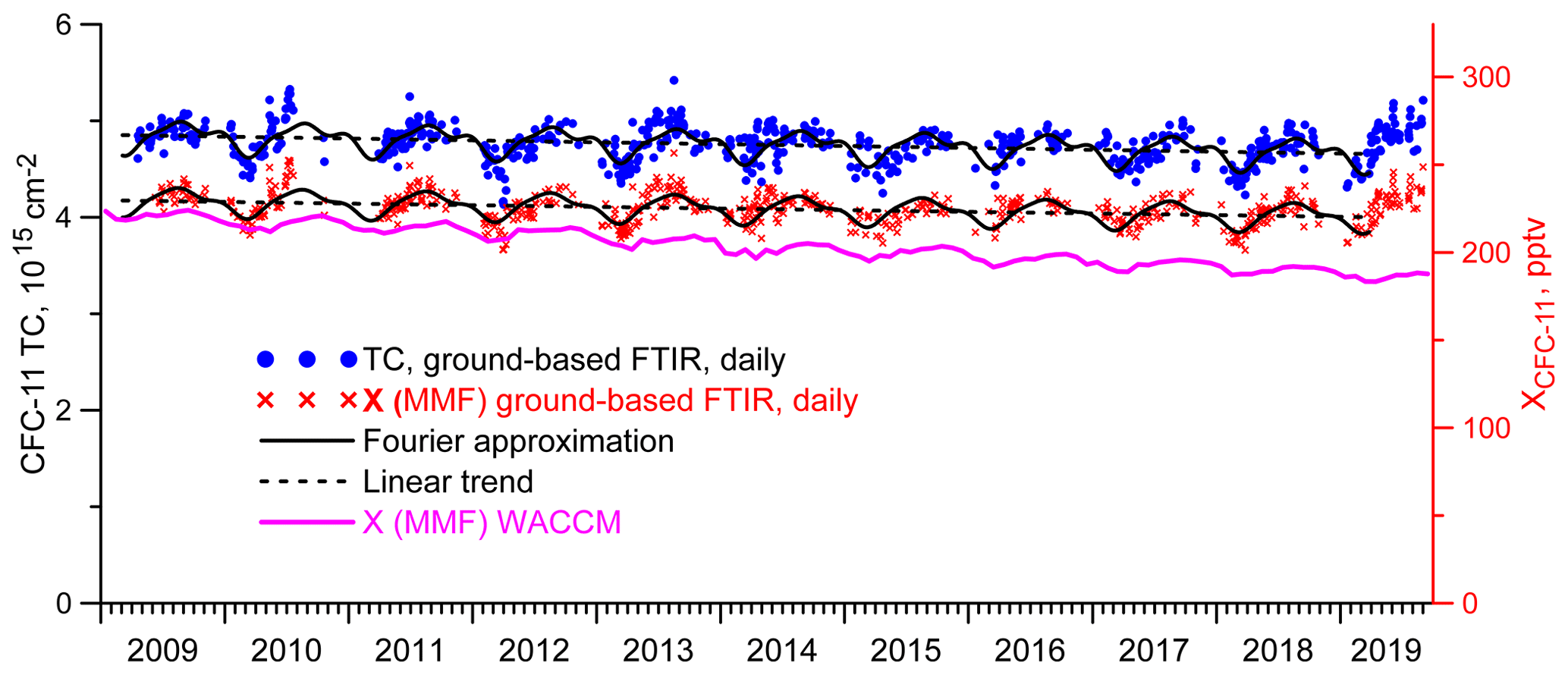
Figures 4–6 show the results in a form of the daily means of both TCs and Xgas. The TC values directly represent the results of spectra inversion, while Xgas values are calculated by dividing the gas total column by the dry air total column. The analysis of Xgas values avoids the influence of the surface pressure and humidity variability, and thus, these values are more stable. To analyze the variability in target gases on a scale of both long-term trends and seasonal variability, we used the approach implemented by Gardiner et al. (2008) for assessing the trends, which is based on the approximation of a series of data by expansion on a finite-dimensional basis; see Eq. (3).

$$\begin{array}{}\text{(3)}& F\left(t\right)\approx a+bt+c_{\mathrm{1}}{f}_{\mathrm{1}}\left(t\right)+c_{\mathrm{2}}{f}_{\mathrm{2}}\left(t\right)\mathrm{\dots }+c_k{f}_k\left(t\right).\end{array}$$

In Eq. (3), F(t) is a dependence approximated by the expansion, in our case represented by discrete measurement data, t is time (years), a is the constant, and b is the linear term coefficient that is equal to a trend value. c_i, i=1, and k are the coefficients, k is the number of coefficients, and f_i(t) are the basis functions. Due to the annual cyclical nature of atmospheric processes, a trigonometric Fourier series with a maximum period of a year is used, which corresponds to the basis functions in Eq. (4), as follows:

$$\begin{array}{}\text{(4)}& f_{\mathrm{2}i-\mathrm{1}}\left(t\right)=\cos \left(\mathrm{2}\mathit{\pi }it\right),f_{\mathrm{2}i}\left(t\right)=\sin \left(\mathrm{2}\mathit{\pi }it\right),i=\mathrm{1},m,\end{array}$$

where m=3 or, which is the same, k=6. Let us write Eq. (3) in the form of Eq. (5), highlighting the nonlinear part S(t) (Eq. 6).

$$\begin{array}{}\text{(5)}& F\left(t\right)\approx a+bt+S\left(t\right),\end{array}$$

where, in the following:

$$\begin{array}{}\text{(6)}& S\left(t\right)=c_{\mathrm{1}}{f}_{\mathrm{1}}\left(t\right)+c_{\mathrm{2}}{f}_{\mathrm{2}}\left(t\right)\mathrm{\dots }+c_k{f}_k\left(t\right).\end{array}$$

S(t) can be considered as being a periodic component of the measurement data time sequence, and its one period can be analyzed as a seasonal data variability. Figures 4–6, in addition to the daily mean values of Xgas and TC, also show, with a dashed line, the linear trend a+bt and, with a solid black line, the result of approximating the measurement data by the trigonometric Fourier series in Eqs. (3) and (4). Figure 4 demonstrates a pronounced periodicity of the results, showing the seasonal variation in both the TCs and Xgas of CFC-11. A similar periodicity is also observed in satellite measurements and in the WACCM data. As expected, Xgas exhibit a slightly smaller scatter than TCs. Note that, starting from April 2019, there is a sharp increase in the concentrations of CFC-11. At present, we have no way of explaining whether such growth is objectively presented or caused by peculiarities in the operation of the instrument. At the same time, this growth noticeably affects the trend estimates. Therefore, when calculating the trends of CFC-11 TCs and Xgas, we limited the CFC-11 time series to April 2019, leaving the analysis of the reasons for this feature outside the scope of this study.

Figure 4 Daily mean TCs and Xgas of CFC-11. The T−Ph parameter α=85.

CFC-12 measurements (Fig. 5) show significantly different results. First of all, the comparison of Figs. 4 and 5 and estimates of the intraday variability and measurement uncertainties of these gases demonstrate that the TCs and Xgas of CFC-12 show less scatter than that of CFC-11, except for some isolated anomalies. The seasonal variability in these values for CFC-12 is noticeably less than that for CFC-11. We also note that, moving from TCs to Xgas, the deviations in the results from the approximating segment of the Fourier series decrease significantly. Variations in surface pressure and water vapor TCs make a significant contribution to the variability in CFC-12 TCs, which indicates small changes in its VMR profile. We analyze these factors in detail in Sect. 3.3.

Figure 5 Daily mean TCs and Xgas of CFC-12. Filtered results of the T−Ph parameter α=85.

Having considered the results of measurements of HCFC-22 daily means, we observed a large variability consistent with a large random component of the total error estimates (see Table 4). There are also noticeable seasonal variations. At first glance, the filter change in February 2016 clearly manifests itself in a change in the data scatter, but in 2016, the scatter looks no less than in previous years and sharply decreases in 2017 and later. Noteworthy is the observed cessation of the increase in HCFC-22 values starting from 2018, previously described by Polyakov et al. (2020a). We also observed an increase in the scatter of the results for all three gases in 2013 due to a decrease in the SNR values caused by the degradation of the tracking system mirror.

Figure 6 Daily mean TCs and Xgas of HCFC-22. Filtered results of the T−Ph parameter $\mathit{\alpha }=\mathrm{3}\times {\mathrm{10}}^{\mathrm{3}}$.

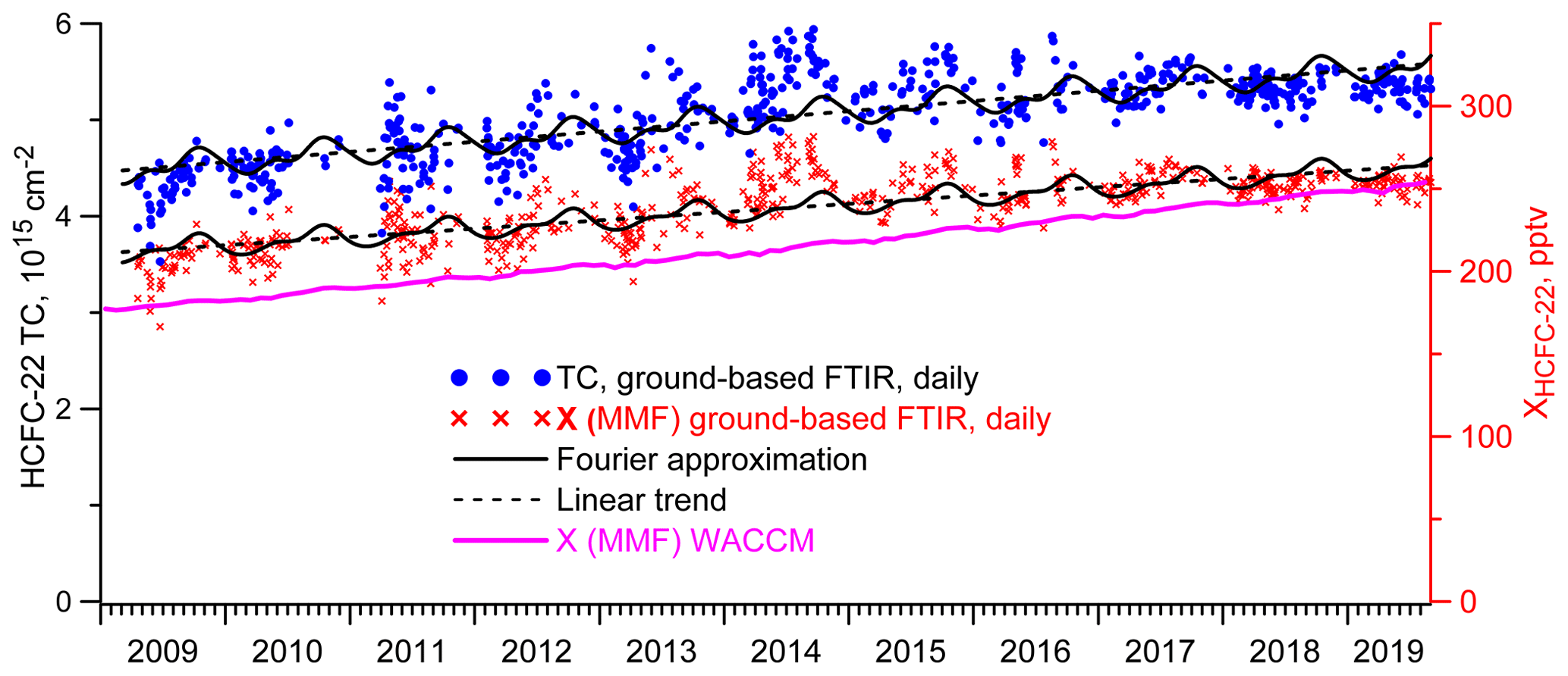
Table 5 presents trend estimates for Xgas time series using two different methods described by Gardiner et al. (2008) and Timofeev et al. (2020). Gardiner et al. (2008) model the intra-annual variability in terms of a Fourier series, and Timofeev et al. (2020) use monthly mean values of the considered period to describe a seasonal cycle. In both methods, trends are estimated by subtracting the seasonal variability from initial time series. In the first method, we consider periodicities of 4 months and larger; in the second method, the monthly mean values account for periodicities from 1 month. The estimation of the width of the confidence interval of the trend value for Gardiner's approach is carried out using the bootstrap method; for Timofeev's method, it is calculated on the basis of a theoretical statistical approach. We do not take the autocorrelation that can be presented in long-lived Xgas time series into account. Santer et al. (2000) demonstrated that neglecting the autocorrelation in a time series could affect the trends estimates and underestimate uncertainties; however, due to substantially irregular FTIR measurements, it was difficult to estimate it.

Gardiner et al. (2008)Timofeev et al. (2020)

Table 5 Estimated trends of Xgas derived from the FTIR measurements at the St. Petersburg site in 2009–2019.

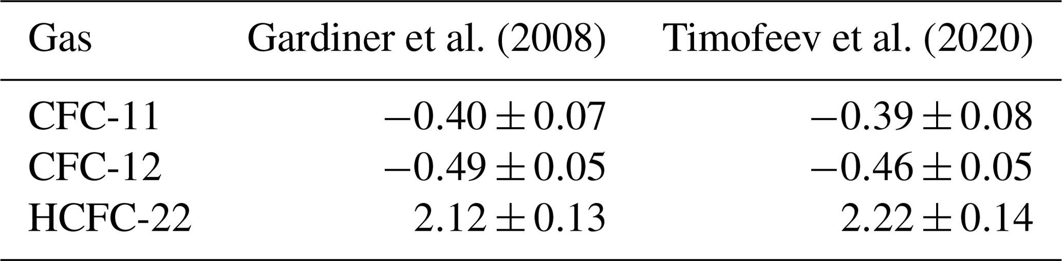
Table 5 demonstrates that the differences between two methods remain within the 95 % confidence interval, i.e., they are not significant.

3.3 Comparison with independent data

We compared the FTIR results at the St. Petersburg site with the data of measurements and modeling. There are three sources of data for the concentration of halocarbons in the atmosphere. First, the in situ measurements at the surface (carried out exactly by the in situ and flask methods) are available from the AGAGE (Dunse et al., 2005) and HATS (Montzka et al., 1993) observational networks; the data are regularly updated at ftp://ftp.cmdl.noaa.gov/hats (last access: 28 June 2020). Measurements are carried out at fixed locations, the closest of which is Mace Head, Ireland (MHD), at a distance of 2500 km and 6.6^∘ south of the St. Petersburg site. The mean values and the trends of Xgas were calculated from the FTIR data and from the MHD site near-ground data for the period (2009–2019) for all three gases. The results are shown in Table 6 in columns 1 and 3. The mean near-ground VMRs (GVMRs) at the MHD site for CFC-11, CFC-12, and HCFC-22 equal 234, 517, and 237 pptv (parts per trillion by volume), whereas the FTIR Xgas measurements show 225, 493, and 252 pptv means, respectively. The trend values (Table 6; columns 2 and 4) for the GVMR data are −0.53, −0.59, and 2.0 % yr⁻¹; for the FTIR data, they are −0.38, −0.48, and 2.0 % yr⁻¹ for CFC-11, CFC-12, and HCFC-22, respectively. Taking into account the spatial discrepancy, the different nature of the measured quantities and the different measurement conditions (background conditions on the Atlantic coast and measurements near the large agglomeration of St. Petersburg), the agreement between the mean values and the trends can be considered satisfactory. It should be noted that the differences in trend estimates do not go beyond the differences in trend values obtained by other researchers. Zhou et al. (2016) obtained trends of −0.86 % yr⁻¹, −0.76 % yr⁻¹, and 2.84 % yr⁻¹ for the period 2009–2016; WMO (2018) indicated that averaged VMRs for 2015 comprised 229.2–231.1, 515.3–519.7, and 233.0–238.0 pptv, and the trends for the period 2010–2016 were −0.70 % yr⁻¹, −0.47 % yr⁻¹, and 2.54 % yr⁻¹ for CFC-11, CFC-12, and HCFC-22, respectively. Taking into account the decrease in both the rate of decay of CFC-11 and the rate of growth of HCFC-22 (e.g., Polyakov et al., 2020a), the agreement of both concentrations and trend values seems to be satisfactory.

The second source of information on the halocarbons content is the satellite measurements, presented most fully for target gases by the ACE-FTS instrument data (for which version 4 is described by Boone et al., 2020). The ACE-FTS is a high spectral resolution (0.02 cm⁻¹) Fourier transform spectrometer operating from 2.2 to 13.3 µm (750–4400 cm⁻¹), based on a Michelson interferometer. The instrument is a main payload on board the SCISAT-1 satellite, with a drifting orbit, an inclination of 73.9^∘, and an altitude of 750 km. Working primarily in the solar occultation mode, the satellite provides information on vertical profiles (typically 10–100 km) for temperature, pressure, and the VMRs of dozens of atmospheric gases over the latitudes of 85^∘ N to 85^∘ S. The lower boundary of the retrieved profiles does not fall below 6 km, but, as a rule, it is above 7–8 km, and the errors at the lower level may be greater than in the rest of the profile. Therefore, we used, for comparisons only, the profiles in which the data were available above 7 km and analyzed the average satellite VMRs (SVMR) in the 8–12 km layer to reduce the random error. For comparison, we selected the ACE-FTS measurements closer than 500 km from the St. Petersburg site. In 2009–2019, there are only 47 d of SVMR measurements for CFC-11 (mean 233 pptv; trend $-\mathrm{0.68}\pm \mathrm{0.23}$ % yr⁻¹), 47 d for CFC-12 (mean 521 pptv; trend $-\mathrm{0.52}\pm \mathrm{0.16}$ % yr⁻¹), and 46 d for HCFC-22 (mean 240 pptv; trend 2.0±0.5 % yr⁻¹). The results are shown in columns 7 and 8 of Table 6. Due to the peculiarity of the orbit and the weather conditions at the St. Petersburg site, SCISAT-1 measurements are available on rare occasions; during 10 years, we have not found more than 47 measurements closer than 500 km to the St. Petersburg site. However, the 95 % probability intervals show the reliability of the trend estimates, using the bootstrap method by Gardiner et al. (2008). As one can see, by comparing columns 1 and 7 of Table 6, the confidence intervals of the means overlap, i.e., the difference in the mean values is not significant only for HCFC-22, and for both CFC-11 and CFC-12, the SVMR is significantly greater than the FTIR Xgas; the difference totals 8 pptv, or 3.5 % for CFC-11 and 28 pptv or 6.3 % for CFC-12. To increase the number of data pairs, we analyzed all ACE-FTS data at all longitudes in the 55–65^∘ N latitudinal range, including the St. Petersburg site (about 60^∘ N). For the period of the FTIR measurements, the SVMR data include 1113 measurements for CFC-11, with the mean of 235.3 pptv and the trend value of −0.63 % yr⁻¹, 1120 measurements for CFC-12 (526.4 pptv, −0.58 % yr⁻¹), and 1111 measurements for HCFC-22 (239.5 pptv, 2.2 % yr⁻¹; see columns 5 and 6 of Table 6).

Table 6 The means and the trends estimates of the FTIR Xgas, GVMR, and SVMR measurements, and the WXgas. If the width of the confidence interval is not specified, then it is less than the last significant digit.

With a 20 times larger data set, the confidence intervals for the trends for the latitudinal range are much narrower than for a circle with a radius of 500 km; thus, differences in the SVMR trends vs. FTIR Xgas trends for CFC-11 and CFC-12 become significant. Such a discrepancy may be due to the different physical nature of the compared quantities. The satellite data do not take into account the lower tropospheric layers, where the influence of anthropogenic pollution sources is the greatest. Therefore, analyzing the trends and deriving from this that the background values of the VMRs for atmospheric CFC-11 and CFC-12 (in situ and satellite) are falling faster than the FTIR Xgas in the industrially developed European part of Russia (near the megacity of St. Petersburg), we may assume that some sources of CFC-11 and CFC-12 exist somewhere there. The absolute values of CFC-11 and CFC-12 FTIR Xgas are smaller than that of the in situ and satellite measurements, but this may only be due to the uncertainty of the spectroscopy used (see the estimates of the systematic in Table 4; row 3).

Figure 7 depicts seasonal variation functions S(t), in Eq. (6), for three gases and for four types of data, i.e., near-ground VMR (GVMR) at the MHD station, satellite mean VMR (SVMR) 8–12 km (55–65^∘ N), the Xgas by FTIR measurements (Xgas), and the Xgas from the WACCM (WXgase).

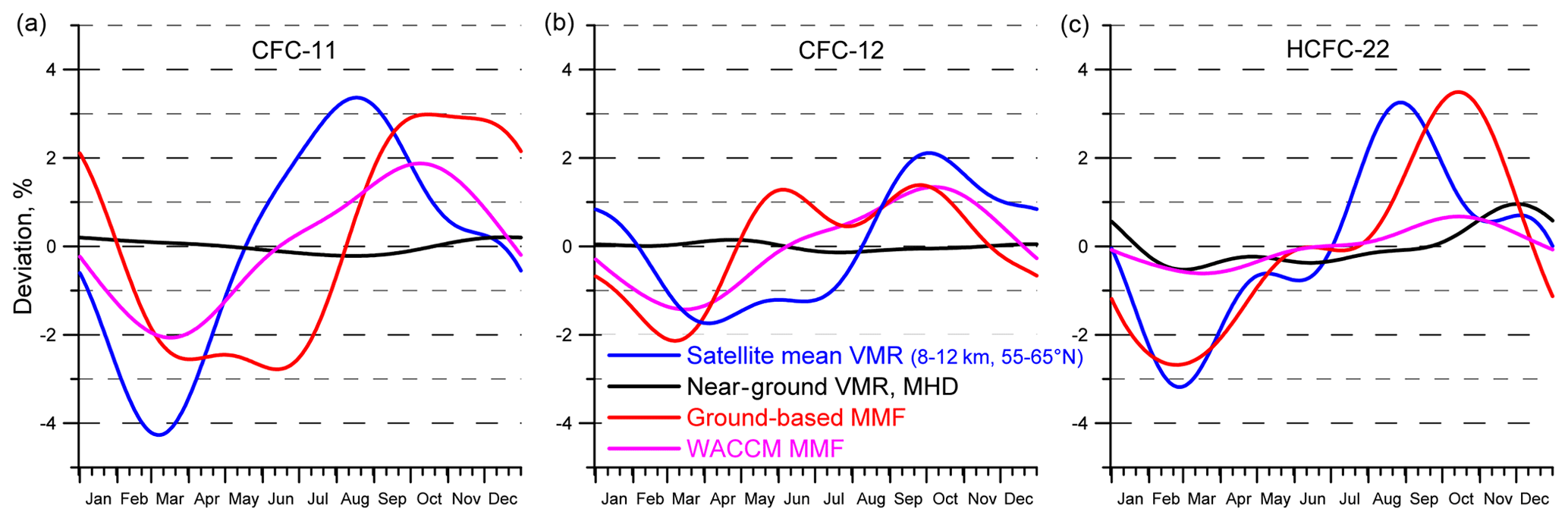
Figure 7 Seasonal relative variability in CFC-11 (a), CFC-12 (b), and HCFC-22 (c). Satellite refers to the ACE-FTS measurements; ground-based and WACCM refer to the FTIR measurements and numerical modeling at the St. Petersburg site.

There are some fundamental differences between local surface and remote sensing measurements (satellite and ground-based FTIR). First, surface measurements are performed regularly and frequently, resulting in stable averages. Second, they are unaffected by variations in pressure and tropopause height. And, finally, the surface data used were obtained in close to background conditions. Therefore, Fig. 7 demonstrates the low seasonal variability in the GVMR, which is within tenths of a percent for CFC-11 and CFC-12 and within 0.7 % for HCFC-22. At the same time, a noticeable seasonal variation in the FTIR Xgas and the SVMR values for all three gases and of the WACCM Xgas for CFC-11 and CFC-12 are observed. The maximal amplitude of the variability reaches 4 % for CFC-11, slightly exceeds 3 % for HCFC-22, and is close to 2 % for CFC-12. For all three gases, seasonal variations in SVMR and Xgas are qualitatively and quantitatively similar; in spring (March–April), there is a minimum, and in late summer or autumn (August–October), there is a maximum. At the same time, there are some differences in the seasonal cycles. For CFC-11, the change in Xgas is 2–3 months ahead of SVMR, while for HCFC-22 the autumn maximum shows the same tendency, whereas the spring minimum, on the contrary, is observed simultaneously for Xgas and SVMR. For CFC-12, the Xgas amplitude is approximately half that for two other gases; the spring minimum of Xgas, on the contrary, is observed before that of SVMR, and the autumn maxima coincide. For CFC-12, a second maximum in the Xgas seasonal cycle is observed in the early summer. WXgas for CFC-11 and CFC-12, on the whole, show a qualitatively and quantitatively similar seasonal variability to Xgas and SVMR, while, on the contrary, for HCFC-22, the changes in WXgas are significantly less (less than 1 %) than that of Xgas and SVMR. In general, we can conclude that Xgas, SVMR, and WXgas show qualitatively similar seasonal variation, with some quantitative differences, and the GVMR variabilities are significantly less. The variability in WXgas for HCFC-22 depicts the only exception; it is essentially less than the Xgas and SVMR variability.

4 Conclusions

1. The retrieval strategies for deriving TCs of CFC-11, CFC-12, and HCFC-22, using ground-based IR solar spectra measurements by the Bruker IFS125HR spectrometer at the NDACC site of St. Petersburg were improved. To solve the inverse problem, values of the regularization parameter of the T−Ph approach were optimized. The time series of TCs and Xgas for CFC-11, CFC-12, and HCFC-22, above the St. Petersburg site near St. Petersburg, Russia in 2009–2019, were obtained. The estimates of the DFS values are 1.05±0.06, 1.20±0.05, and 1.00±0.00; the estimates of the relative systematic and random errors are 7.61 % and 3.08 %, 2.24 % and 2.40 %, and 5.75 % and 3.70 %, for CFC-11, CFC-12, and HCFC-22, respectively.

2. Mean values of X_CFC-11, X_CFC-12, and X_HCFC-22 are 225, 493, and 238 pptv. The RMS intraday variability in TCs of measured gases is 0.8 %, 0.6 %, and 2.3 % for the three gases in the same order. Estimates of the Xgas trends of CFC-11, CFC-12, and HCFC-22 equal $-\mathrm{0.40}\pm \mathrm{0.07}$ % yr⁻¹, $-\mathrm{0.49}\pm \mathrm{0.05}$ % yr⁻¹, and 2.12±0.13 % yr⁻¹, respectively. The analysis of the seasonal variability in CFC-11, CFC-12, and HCFC-22 demonstrates the similar qualitative seasonal variability for all three gases, with a minimum in spring–early summer and a maximum in fall; X_CFC-11 and X_HCFC-22 variability amounts to 3 %, and the variability in X_CFC-12 amounts to 2 %.

3. Mean values, trends, and the seasonal variability in X_CFC-11, X_CFC-12, and X_HCFC-22 above the St. Petersburg site were compared to the same parameters of the near-ground VMRs measured at the site in Mace Head, Ireland. It is shown that the mean of X_CFC-11 above the St. Petersburg site is 9 pptv (3.8 %) less than the mean GVMR at the MHD site, the mean of X_CFC-12 is 24 pptv (4.6 %) less than the mean GVMR, and the mean of X_HCFC-22 does not significantly differ from the mean GVMR. In absolute values, the trend of X_CFC-11 is 0.13 % yr⁻¹ less (−0.40 vs. −0.53 % yr⁻¹) than that of the GVMR, the trend of X_CFC-12 is 0.10 % yr⁻¹ less (−0.49 % yr⁻¹ vs. −0.59 % yr⁻¹) than that of the GVMR, and the trend of X_HCFC-22 does not significantly differ from that of GVMR (2.12±0.13 % yr⁻¹ vs. 2.0±0.05 % yr⁻¹). The seasonal variability in GVMR for all three gases is much lower than the Xgas variability.

4. Mean values, trends, and the seasonal variability in X_CFC-11, X_CFC-12, and X_HCFC-22 above the St. Petersburg site were compared to the same parameters of SVMR. SVMR stands for the mean values of VMR, measured with ACE–FTS between altitudes of 8–12 km and between latitudes of 55–65^∘ N. It is shown that the mean X_CFC-11 is 10 pptv (4.3 %) less than the mean SVMR, the mean X_CFC-12 is 33 pptv (6.3 %) less than the mean SVMR, and the mean X_HCFC-22 is 2 pptv (0.8 %) less than the mean SVMR. In terms of the absolute value, the X_CFC-11 trend is 0.23 % yr⁻¹ less (−0.40 % yr⁻¹ vs. −0.63 % yr⁻¹) than the trend of SVMR, the trend of X_CFC-12 is 0.09 % yr⁻¹ less than the trend of SVMR (−0.49 % yr⁻¹ vs. −0.58 % yr⁻¹), and the trend of X_HCFC-22 does not significantly differ from that of SVMR (2.12±0.13 vs. 2.2 % yr⁻¹). Xgas and SVMR show qualitatively and quantitatively similar seasonal variations.

5. Mean values, trends, and seasonal variability in X_CFC-11, X_CFC-12, and X_HCFC-22 were compared to the same parameters of WXgas. WXgas stands for Xgas calculated on the basis of the WACCM data set of the VMR profiles for the St. Petersburg site. It is shown that the mean X_CFC-11 is 22 pptv (10 %) greater than the mean WX_CFC-11, the mean X_CFC-12 is 15 pptv (3.1 %) greater than the mean WX_CFC-12, and the mean X_HCFC-22 is 23 pptv (10 %) greater than the mean WX_HCFC-22. In terms of the absolute value, the X_CFC-11 trend is 1.28 % yr⁻¹ less than the trend of WX_CFC-11 (−0.40 % yr⁻¹ vs. −1.68 % yr⁻¹), the trend of X_CFC-12 is 0.35 % yr⁻¹ less than the trend of WX_CFC-12 (−0.49 % yr⁻¹ vs. −0.84 % yr⁻¹), and the trend of X_HCFC-22 is 1.28 % yr⁻¹ less than the trend of WX_CFC-22 (2.12 % yr⁻¹ vs. 3.40 % yr⁻¹). Xgas and WXgas show qualitatively and quantitatively similar seasonal variations for CFC-11 and CFC-12; the seasonal variability in the WX_HCFC-22 is essentially less than X_HCFC-22 variability.

In general, the comparison of the FTIR Xgas with the independent data shows a good agreement of their means within the systematic error of the measurements. The trends observed over the St. Petersburg site demonstrate the smaller decrease rates for CFC-11 and CFC-12 than the independent data and the same increase rate for HCFC-22.

Appendix A: Spectra samples

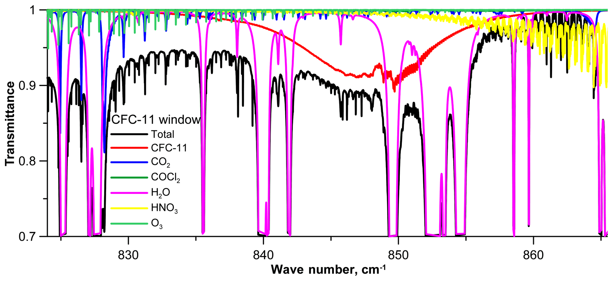
Figure A1 Absorption by various gases in the spectral region of the CFC-11 absorption band (7 November 2017, 09:57 UTC; SZA is 76^∘).

Figure A2 Absorption by various gases in the spectral region of the CFC-12 absorption band (1160 cm⁻¹; 19 June 2017, 10:25 UTC; SZA is 37^∘).

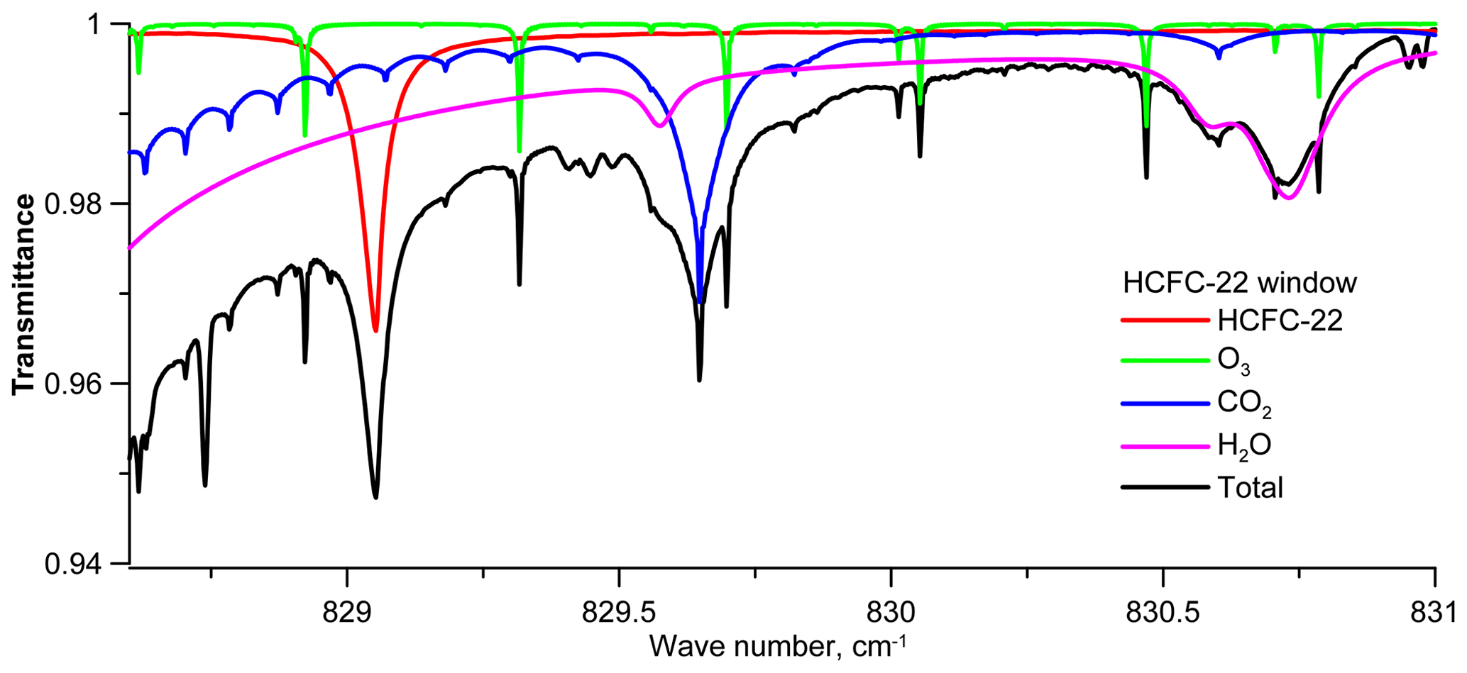
Figure A3 Absorption by various gases in the spectral region near the HCFC-22 absorption line (829 cm⁻¹; 19 June 2017, 10:25 UTC; SZA is 37^∘).

Appendix B: Results filtering

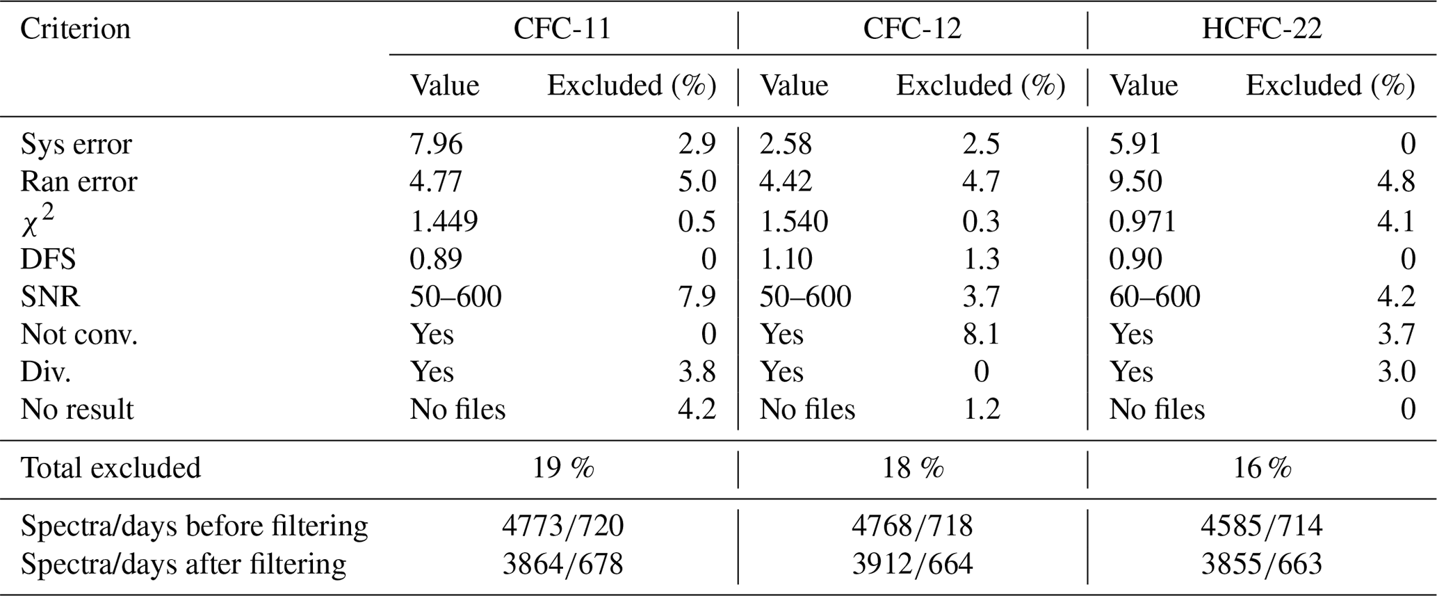
We filtered the retrieved TCs using the following criteria. The SNR of measured spectra should be in the range of 50–600, and the deviation from the mean statistical characteristics presented in Table 2 should not be greater than 2 times the SD. The criteria used and the percentage of the measurements discarded after their application are shown in Table B1.

Table B1 The criteria used and the percentage of data discarded after their application.

Legend for the rows of Table B1:

1. Systematic error (mean plus 2 SD)

2. Random error (mean plus 2 SD)

3. Residual (χ²) (mean plus 2 SD)

4. DFS (mean minus 2 SD)

5. To exclude noisy spectra and possible nonlinearity in measurements, we use only measurements with SNR values ranging from 50 (60) to 600.

6. Not converged

7. Divergence warning

8. SFIT4 did not present results