the Creative Commons Attribution 4.0 License.
the Creative Commons Attribution 4.0 License.
 | 17 Aug 2021
Something fishy going on? Evaluating the Poisson hypothesis for rainfall estimation using intervalometers: results from an experiment in Tanzania
Didier de Villiers
Marc Schleiss
Marie-Claire ten Veldhuis
Nick van de Giesen
A new type of rainfall sensor (the intervalometer), which counts the arrival of raindrops at a piezo electric element, is implemented during the Tanzanian monsoon season alongside tipping bucket rain gauges and an impact disdrometer. The aim is to test the validity of the Poisson hypothesis underlying the estimation of rainfall rates using an experimentally determined raindrop size distribution parameterisation based on Marshall and Palmer (1948)'s exponential one. These parameterisations are defined independently of the scale of observation and therefore implicitly assume that rainfall is a homogeneous Poisson process. The results show that 28.3 % of the total intervalometer observed rainfall patches can reasonably be considered Poisson distributed and that the main reasons for Poisson deviations of the remaining 71.7 % are non-compliance with the stationarity criterion (45.9 %), the presence of correlations between drop counts (7.0 %), particularly at higher arrival rates (ρa>500 ), and failing a χ2 goodness-of-fit test for a Poisson distribution (17.7 %). Our results show that whilst the Poisson hypothesis is likely not strictly true for rainfall that contributes most to the total rainfall amount, it is quite useful in practice and may hold under certain rainfall conditions. The parameterisation that uses an experimentally determined power law relation between N0 and rainfall rate results in the best estimates of rainfall amount compared to co-located tipping bucket measurements. Despite the non-compliance with the Poisson hypothesis, estimates of total rainfall amount over the entire observational period derived from disdrometer drop counts are within 4 % of co-located tipping bucket measurements. Intervalometer estimates of total rainfall amount overestimate the co-located tipping bucket measurement by 12 %. The intervalometer principle shows potential for use as a rainfall measurement instrument.
- Article
(4902 KB) - Full-text XML
- BibTeX
- EndNote


Africa, and particularly Sub-Saharan Africa, is one of the most vulnerable regions in the world to climate change (Boko et al., 2007). The main economic activity (by share of labour) is agriculture, with 98 % of crop production being rainfed (Abdrabo et al., 2014). At the same time, much of Sub-Saharan Africa is greatly underserviced by weather observations, and the existing observational networks have been in decline since the mid-1990s; from an average of eight stations per 1 million square kilometres, the density has decreased to less than one in 2015 (data from the Climate Research Unit of the University of East Anglia, 2017). There are some organisations working on setting up new observational networks, such as the Trans-African Hydro-Meteorological Observatory (TAHMO), but progress is slow due to the lack of financial incentives for weather data. As a result, the African climate has not been as well researched in comparison to those of western Europe and the United States (Otto et al., 2015; Washington et al., 2006).
For example, a recent review of weather index insurance for smallholder farmers (some of the world's poorest people) found that the sparsity of ground-based weather stations is a large challenge for insurers in Sub-Saharan Africa (Greatrex et al., 2015), and companies have been forced to look to other sources of data or to develop other indices by which to insure crops. Global rainfall estimates from satellites, such as the Global Precipitation Measurement (GPM) mission, are instrumental in bridging this gap. However, satellite observations, whilst providing good spatial coverage, do not cover the entire temporal period, and the spatial resolution is often too coarse for local applications. Robust, inexpensive and accurate rainfall measuring instruments would add a lot of value by providing ground-based measurements.
Satellite retrievals face another issue for areas with a lack of ground-based data for validation. Since both active (radars) and passive (radiometers or IR sensors) onboard sensors do not measure rainfall directly, information about the microstructure of precipitation is needed in order to develop robust rainfall retrieval algorithms. Information about the drop size distribution (DSD) in particular is needed to retrieve rainfall rates (R) from radar reflectivity (Z) measurements observed by, e.g. radars aboard the GPM mission (Munchak and Tokay, 2008; Guyot et al., 2019). A foundational work in this regard is the exponential DSD model proposed by Marshall and Palmer (1948). Since then, a lot of work has been done on determining alternative parameterisations and many different models have been proposed, of which the most widely used are the exponential, gamma (Ulbrich, 1983; Tokay and Short, 1996; Iguchi et al., 2017) and lognormal distributions (Feingold and Levin, 1986). It has also been shown that the appropriate parameterisation is dependent on the type of rainfall (Atlas and Ulbrich, 1977) and the climatic setting (Battan, 1973; Bringi et al., 2003). Therefore, ground “truthing” of DSDs for satellite retrievals is very important to ensure that the natural variability of the DSD is being correctly taken into account when estimating rainfall rates (Munchak and Tokay, 2008).
An assumption that is seldom explicitly mentioned in the presentation of these parameterisations is the homogeneity assumption (Uijlenhoet et al., 1999), which states that below some minimum scale, raindrops are distributed homogeneously (as uniformly as randomness allows) in space and time. Otherwise, the parameterisation would depend on the size of the sample volume, area and/or time period to which it pertains. Statistical homogeneity implies that the number of drops in a fixed volume can be described by a single constant parameter such as the average drop density per unit volume or the raindrop arrival rate at the surface (Uijlenhoet et al., 1999). Such a point process is called a homogeneous or stationary Poisson point process, and the number of drops is distributed according to a Poisson distribution (Uijlenhoet et al., 1999). The arrival of raindrops at a surface has long been considered an example of a Poisson process (Kostinski and Jameson, 1997; Joss and Waldvogel, 1969). However, this assumption has been questioned and several studies argue that the homogeneity assumption is incompatible with the spatial and temporal clumping of raindrops that is observed in reality. To borrow Kostinski and Jameson (1997)'s words: “The `streakiness' that is part of the lived experience of rainfall can be seen when sheets of rain pass across the pavement during thunderstorms.” This clumping results in greater variability than is predicted by the Poisson hypothesis.
To overcome these difficulties, two different approaches have been proposed. Some researchers (e.g. Lovejoy and Schertzer, 1990; Lavergnat and Golé, 1998) proposed to abandon the Poisson process framework and replace it with a scale-dependent, multi-fractal representation of rain. Others proposed to generalise the homogeneous Poisson process (with a constant mean) to a doubly stochastic Poisson process or Cox process, where the mean itself is a random variable (Jameson and Kostinski, 1998; Smith, 1993; Cox and Isham, 1980).
The aim of this study is to formally assess the adequacy of the homogeneous Poisson hypothesis and its importance in deriving rainfall estimates from ground-based measurements in a tropical climate. The intervalometer, a new kind of inexpensive rainfall sensor, is introduced and tested for its suitability in providing ground-based rainfall estimates in Sub-Saharan Africa. To this end, nine intervalometers were deployed over a 2-month period during the Tanzanian tropical monsoon. The Marshall and Palmer (1948) exponential parameterisation as well as two other experimentally determined exponential parameterisations of the DSD were used to convert the intervalometer raindrop arrival rates into rainfall rates and results were compared with disdrometer and tipping bucket measurements. A hierarchical system of statistical tests on the drop counts was used to assess the validity of the homogeneous Poisson hypothesis. Section 2 presents the experimental setup. The methods of analysis are detailed in Sect. 3, and the results and discussion are presented in Sects. 4 and 5, respectively. A list of conclusions follows in Sect. 6.
2.1 Instruments
In total, the experiment made use of nine intervalometers, one acoustic disdrometer and two tipping bucket rain gauges at eight different sites. The tipping bucket rain gauge was made by Onset (more info at https://www.onsetcomp.com/products/data-loggers/rg3, last access: 11 August 2021) in the US and was equipped with a HOBO data logger; the acoustic disdrometer was manufactured by Disdrometrics in Delft, the Netherlands; and the intervalometer was also made by Disdrometrics. The intervalometer is a device that registers the arrival of raindrops at the surface of a piezoelectric drum and can be constructed for less than USD 150. It has a minimum detectable drop diameter (Dmin) of 0.8 mm, determined in a lab experiment by Jan Pape. Typical values of Dmin for impact disdrometers are between 0.3 and 0.6 mm (Johnson et al., 2011). The Dmin value of 0.8 mm for the intervalometer means that the instrument is likely to miss many small drops and underestimate rainfall rates. The advantage of the intervalometer over a standard rain gauge is that it provides drop counts as well as rainfall estimates. More information about the intervalometer can be found at https://github.com/nvandegiesen/Intervalometer/wiki/Intervalometer (last access: 11 August 2021). A similar instrument in terms of acoustic sensor is also described by Hut (2013). The acoustic disdrometer registers the kinetic energy of drop impacts at a drum and converts this to an estimate of the drop size. It is similar to an intervalometer but also provides individual drop size estimates. The minimum detectable drop diameter for the disdrometer was thought to be 0.6 mm but in practice was 1 mm. This is larger than what is typical for an impact disdrometer and means that it likely misses many small drops and underestimates the actual rainfall rate. The effect of truncation on rainfall estimation is discussed in Sect. 3.2. A good discussion of the pros and cons of impact disdrometers in general can be found in, e.g. (Tokay et al., 2001; Guyot et al., 2019) and for tipping buckets in, e.g. Ciach (2003). The tipping bucket rain gauge collects all drops over a known surface area and funnels them to a small bucket which tips whenever a fixed volume of water has been collected (typically 0.2 mm). The volume of each tip is verified in situ via a field calibration experiment.
2.2 Experiment
In total, eight sites were selected along the southern coast of Mafia Island, Tanzania. Figure 1 presents the experimental layout. Sensors were placed in an approximate line, such that a rectangle 3.1 km in length and 500 m in width would cover all the sites. The dimension of the long axis of the experiment was chosen to approximate that of the spatial resolution (approximately 5 km) of the GPM dual polarisation radar (DPR) instrument.
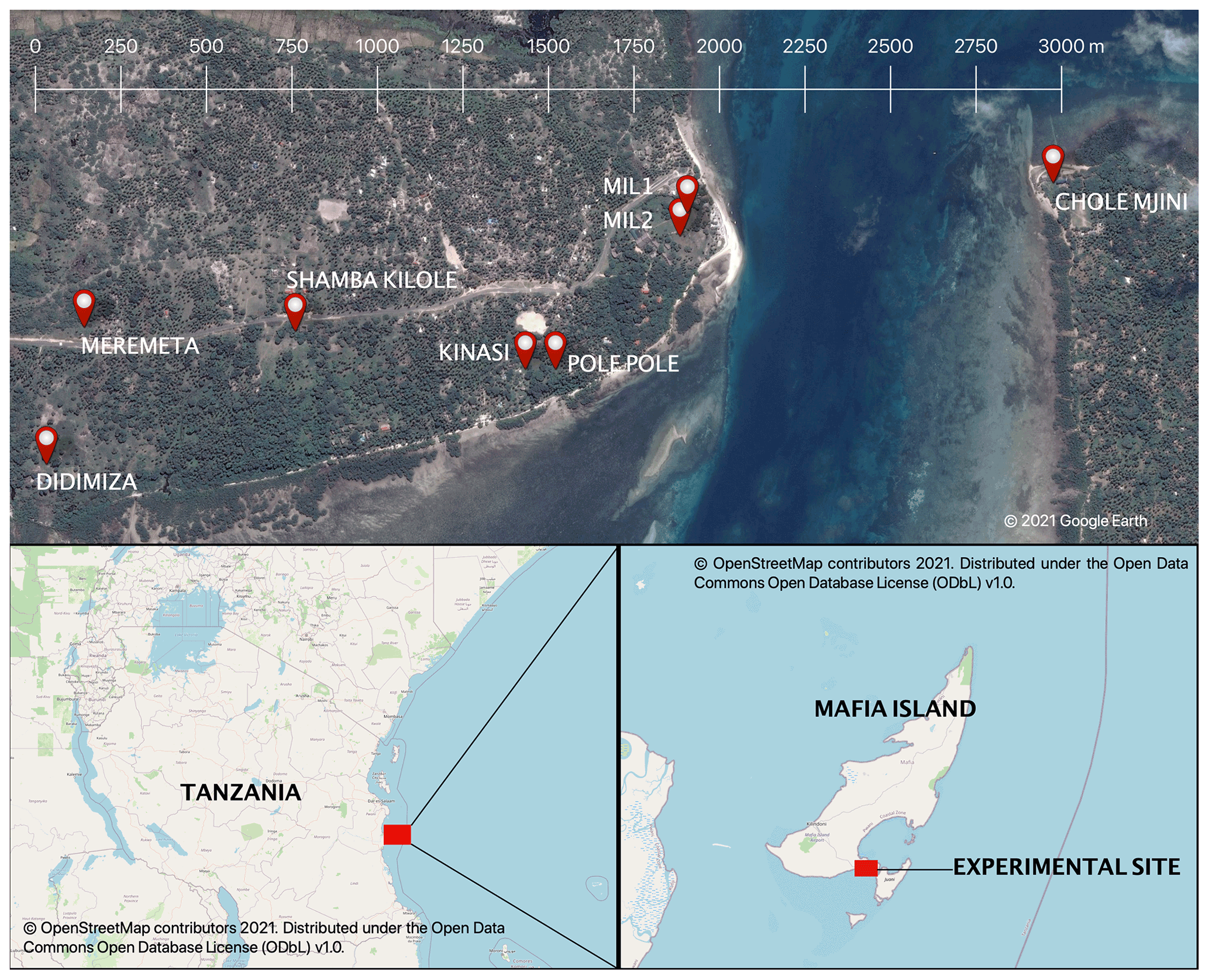
Figure 1The eight intervalometer sites on Mafia Island, off the coast of Tanzania. Each site contains one intervalometer. Pole Pole also had a co-located tipping bucket and impact disdrometer. MIL1 also had a co-located tipping bucket.
Rainfall measurement sites were chosen to comply as much as possible with World Meteorological Organisation guidelines within the constraints of accessibility and landscape. Ideally, this means that all of the sensors should be placed in vegetation clearings, sheltered as much as possible from the wind at a height of 1.5 m off the ground and 1.5 m to the nearest instrument (if co-located) and between 2×H and 4×H from the nearest object, where H is the difference in height between the nearest obstacle and the rainfall measurement instrument. All guidelines were followed except for the H requirement due to dense vegetation within the entire observational area. In practice, the distance to the nearest object ranged between H and 4×H. No instruments where placed at sites where the nearest obstacle was ≤H away. Tipping buckets were calibrated in the field by dripping 100 mL of water (from a tripod stand) at a rate slower that 20 mm h−1 onto the instrument and recording the number of tips. The calibration experiment was repeated five times for each tipping bucket to determine the mean volume and the standard deviation (hereafter called SD error) of each tip in the field. At higher rainfall rates than 20 mm h−1, the rainfall accumulation amounts may be underestimated (Humphrey et al., 1997).
2.3 Data availability
There were some issues over the course of the experiment with the various instruments that affected the availability of data. The disdrometer picked up on a oscillating signal from 20 May 2018 onward that resulted in total corruption of the data. Some intervalometers experienced water damage, particularly in storms with high rainfall intensities, which caused the instruments to go offline for certain periods of time. Two were damaged beyond repair. The tipping bucket gauges experienced no known issues. Figure 2 presents an overview of the data available.
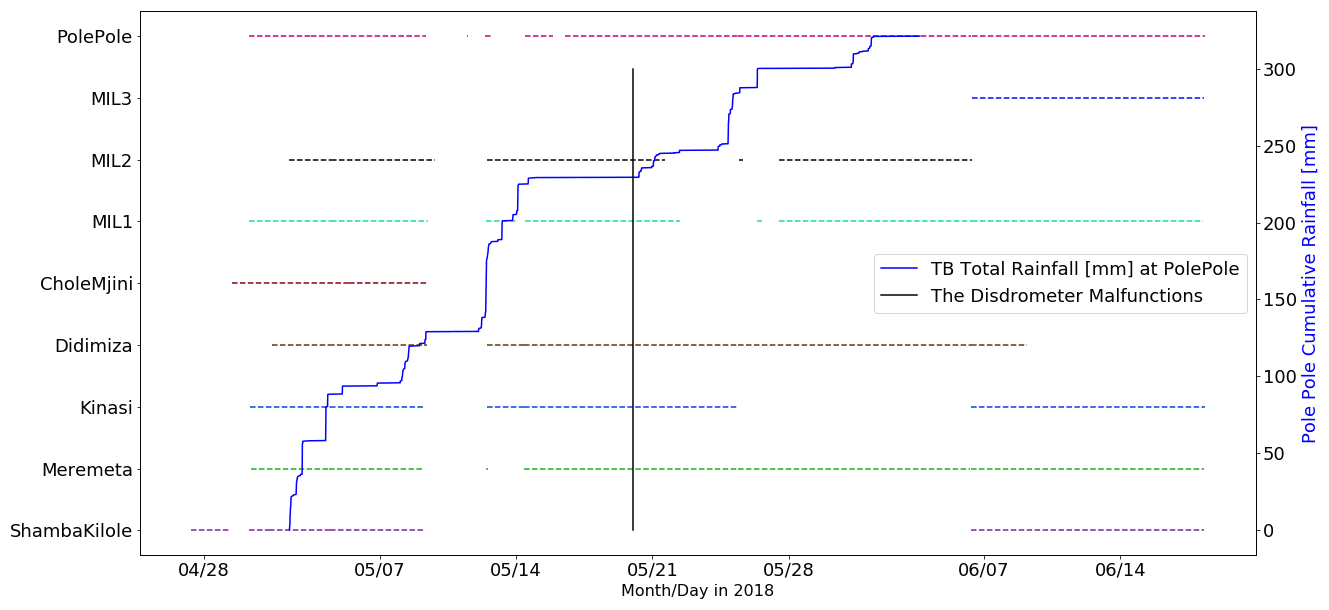
Figure 2Record of the time periods during which the intervalometers collected data for each intervalometer site and the total rainfall amount [mm] from the tipping bucket at Pole Pole.
3.1 Deriving rainfall rates from rain drop arrival rates
Uijlenhoet and Stricker (1999) present an excellent review of the exponential DSD parameterisation as well as the derivations of relevant rainfall quantities. A small summary mostly derived from their work is presented below. The raindrop size distribution in a volume of air NV(D) [] is defined such that the quantity NV(D)dD represents the average number of drops with diameters between D and D+dD per unit volume of air. Marshall and Palmer (1948) proposed to model NV(D) using an exponential model of the form:
If raindrops are assumed to fall at terminal velocity, then NV(D) can be related to the DSD of drops arriving at a unit surface area, NA(D) [], by v(D) [m s−1], which describes the relationship between drop diameter and terminal fall velocity. NA(D) is the form of the DSD that is observed by disdrometers and intervalometers (Uijlenhoet and Stricker, 1999; Smith, 1993).
Atlas and Ulbrich (1977) showed that v(D) can be approximated by a power law, v(D)=αDβ, with α=3.778 [] and β=0.67 [–] providing a close fit to the data collected on the terminal fall velocity of drops in stagnant air by Gunn and Kinzer (1949) for mm. The mean raindrop arrival rate, ρA [], is defined as the integral over all drop sizes of NA(D). For the intervalometer, this is the integral between Dmin=0.8 mm and ∞ since the instrument has a minimum detectable drop diameter of 0.8 mm.
where Γ is the upper incomplete gamma function (Arfken et al., 2013). Uijlenhoet and Stricker (1999) presented an equation relating the rainfall rate (R) to and N0, and noted that for self-consistency purposes the left- and right-hand sides of Eq. (6) should be equal:
This equation can be inverted to give the self-consistent Λ–R relation. If the DSD is truncated (in this case at Dmin), then Eq. (6) is modified as follows:
For the truncated DSD, the Λ–R relation must be solved for numerically. Equation (7) is used in conjunction with the α and β values presented by Atlas and Ulbrich (1977) and the Marshall and Palmer (1948) N0 value and a Dmin of 1 mm. The rainfall rate is varied from 0.1 to 100 mm h−1 in increments of 0.1 mm h−1 and for each value of R, Λ is solved for numerically. The approximate Λ–R power law relation is derived from a best fit of the Λ–R data points and is presented in Eq. (8):
Using the Atlas and Ulbrich (1977) α,β values and the modified R–Λ relationship in Eq. (8), the rainfall rate (R) can then be calculated from the drop arrival rate (ρA). The values of and Dmin are fixed and for a given value of ρA, Eq. (5) is used to numerically solve for . The rainfall rate (R) can be estimated by re-arranging the Λ–R relation in Eq. (8) so that .
3.2 Experimentally determined drop size distribution parameterisations
Sources of measurement error for the intervalometer are the calibration of the parameter Dmin and the measurement of ρA. Errors in the determination of Dmin affect the ρA–R relationship. Errors in the ρA measurement can result from splashing of drops from outside the sensor onto the sensor surface during high-intensity rainfall (resulting in overestimated rain rates), spurious signals from something other than rain falling on the sensor (resulting in overestimated rain rates) or from edge effects (resulting in underestimated rain rates). Edge effects occur when drops with D>Dmin land near the edges of the sensor, where the signal is damped and may not be recorded properly, especially if D is close to Dmin.
There is also model error that arises from the assumption that the DSD is adequately described by the Marshall and Palmer (1948) exponential parameterisation rather than some other parameterisation. The parameterisation of the DSD with a fixed intercept parameter (N0=8000 []) and a slope parameter Λ depending on rain rate according to a power law ( [mm−1]), such as proposed by Marshall and Palmer (1948) derived from stratiform rainfall in Montreal, Canada, may not be applicable in Tanzanian rainfall, which is of a largely convective nature. Model error will be accounted for by comparing three Marshall and Palmer (1948) type exponential parameterisations of the DSD. Many parameterisations for the DSD have been proposed and tested in the literature, of which the most widely used are the exponential (of which the Marshall and Palmer, 1948 model is a special case), gamma (Ulbrich, 1983; Tokay and Short, 1996; Iguchi et al., 2017) and lognormal distributions (Feingold and Levin, 1986). These other parameterisations will not be investigated as the focus of this study is to test the homogeneity assumption that underlies these models rather than compare different DSD parameterisations.
Three separate exponential parameterisation are tested. First is the self-consistent Marshall and Palmer (1948) parameterisation with the Λ–R relation presented in Eq. (8). The second model uses an experimentally determined value for the intercept parameter N0 over the entire observational period. This can be determined from a linear fit of the drop diameter (D) vs. the natural logarithm of NVD for the entire observational period. The experimentally determined value of N0 is 4342 [] and the corresponding self-consistent Λ–R relation is .
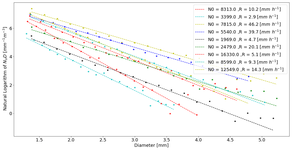
Figure 3The natural logarithm of NVD is plotted against diameter (D) for different rainfall events as well as the linear line of best fit. Each rainfall event has a different value for N0 within the observational period. Note that the data should not be extrapolated to the y axis as the x axis is truncated.
The third model uses a power law to relate the intercept parameter N0 to the rainfall rate. Waldvogel (1974) found that the value of N0 can vary greatly depending on the rainfall event and even within rainfall events. These “jumps” in N0 mean that an average N0 value for the entire observational period may not be sufficient to accurately describe the DSD between or within rainfall events. In that case, the value of N0 for each rainfall event is determined from a linear fit of the drop diameter (D) vs. the natural logarithm of NVD for the rainfall event as shown in Fig. 3. The observed values of N0 vary from less than 2000 [] to more than 15 000 [] within the different rainfall events. A power law is fit to the R vs. N0 values for the different rainfall events and results in the following relation:
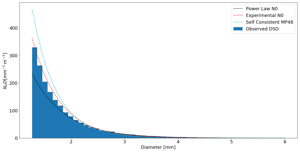
Figure 4The observed DSD over the entire observational period of the disdrometer is compared to the three parameterisations of the DSD. The self-consistent Marshall and Palmer (1948), the experimentally determined N0=4342 [] and the experimentally determined power law of N0. Note that the data should not be extrapolated to the y axis as the x axis is truncated.
The self-consistent Λ–R relation for Eq. (9) is . These two relations form the basis of the experimentally determined power law parameterisation. The three parameterisations as well as the observed DSD are plotted in Fig. 4.
It should be noted that the value of Dmin for both the intervalometer (0.8 mm) and disdrometer (1 mm) is larger than is typical for impact disdrometers. This means that many small drops will not be counted towards the rainfall arrival rate or rainfall rate, resulting in underestimates. Ulbrich (1985) developed a method for estimating the effects of the truncation of the DSD on two rainfall integral variables, the liquid water content and the reflectivity factor. These variables were chosen because they are a function of integer powers of the drop diameter, D3 and D6, respectively. Ulbrich (1985) presents a contour diagram showing the ratio of the rainfall integral variables, with a truncated DSD, to the same rainfall integral variable, without any truncation of the DSD, as a function of the integration limits ΛDmin and ΛDmax. The rainfall rate (R) is not a function of an integer power of the drop diameter, and therefore the integration limits ΛDmin and ΛDmax are approximations for this rainfall integral variable. Ulbrich (1985) shows that the simple approximation still gives excellent results for the rainfall rate. The approximation is used to investigate the effect of DSD truncation on the rainfall rate derived from the disdrometer data. The ratio (Rratio) of the truncated DSD rainfall rate to the rainfall rate without truncation effects is given by the ratio of Eqs. (7) to (6). This simplifies to Eq. (10).
Ratios of 0.8, 0.9 and 0.95 (i.e. an underestimate within 5 %) correspond to ΛDmin values of 2.8, 2.2 and 1.8, respectively. For the disdrometer (Dmin=1 mm), this means that any values of Λ>2.8, 2.2 or 1.8 will result in rainfall estimates that are within 20 %, 10 % or 5 %, respectively, of the “true” rainfall rate. These threshold values for Λ can be used to calculate threshold rainfall rates using each of the three Λ–R relations presented for the three exponential parameterisations. At the 95 % level, the threshold rainfall rates for the self-consistent Marshall and Palmer (1948), experimentally determined N0 and the N0 power law are 55.0, 28.3 and 13.4 mm h−1, respectively. At the 90 % level these values decrease to 20.5, 10.6 and 7.2 mm h−1, respectively, and for the 80 % level they decrease still further to 6.2, 3.2 and 3.4 mm h−1, respectively. All observed rainfall rates greater than the threshold rate will be affected by the effects of truncation by less than 20 %, 10 % and 5 %, respectively. During the course of the observational period of the disdrometer, 61.1 % of the total rainfall amount fell at a rainfall rate greater than 13.4 mm h−1 and 82.6 % of the total rainfall amount fell at a rainfall rate greater than 7.2 mm h−1. This means that the majority of the observed rainfall fell at rainfall rates greater than the 90 % ratio level for both the experimentally determined N0 and the N0 power law parameterisations and greater than the 95 % level for the N0 power law parameterisation. Therefore, the contribution of DSD truncation to the error in rainfall estimates of these models is expected to be minimal for the N0 power law and small (<10 %) for the experimentally determined N0 parameterisation. This is not the case for the self-consistent Marshall and Palmer (1948) model which is expected to significantly underestimate the rainfall amount as a result of truncation of the DSD at 1 mm. Since the Dmin of the intervalometer is less than that for the disdrometer, the effect of truncation is even lower.
3.3 The Poisson homogeneity hypothesis
The concept of a drop size distribution depends on the assumption that at some minimum spatial or temporal scale (the primary element) the rainfall process is homogeneous. Homogeneity in a statistical sense implies that the data within the primary element follow Poisson statistics (Uijlenhoet and Stricker, 1999). In particular, some key assumptions must hold:
-
The rainfall process is stationary; i.e. it has a constant mean raindrop arrival rate.
-
The number of raindrops arriving at the surface over non-overlapping time intervals is statistically independent.
-
The number of raindrops arriving at a surface during a time interval [] is proportional to δt.
-
The probability of more than one raindrop arriving at a fixed surface over a time interval [] becomes negligible for δt→0.
Assumptions 3 and 4 are reasonable for small spatial and temporal scales, and 1 and 2 can be tested. If these fundamental assumptions hold then the distribution of raindrops is given by (Feller, 2010)
where μ is the average number of drops arriving at a surface per unit time and k is the random number of drops observed during a particular counting interval/window of time. Kostinski and Jameson (1997) show that this simple Poisson model does not explain the clumpiness that is sometimes observed in real rainfall. However, if μ varies in time and space, then a rainfall event can always be subdivided into N smaller patches, each of which has its own constant μ. In order to derive the total probability density function (PDF) of the drop counts, it is then necessary to integrate over the probability distribution of the patches f(μ), resulting in a Poisson mixture.
The variance of the Poisson mixture is greater than the variance of a pure Poisson PDF. Kostinski and Jameson (1997) show that the Poisson mixture provides a better description of the frequency of drop arrivals per unit time than a simple Poisson model. The definition of f(μ) in Eq. (12) implies that there is a coherence time (τ) over which μ can be considered stationary and to which the homogeneity Poisson hypothesis can be applied. Therefore, in order to estimate f(μ) with sufficient accuracy, one requires (), where T is the entire length of a rainfall event, τ is the coherence time of a patch and t is the counting interval for the raindrops. Kostinski and Jameson (1997) showed that an order of magnitude difference is sufficient between t,τ and τ,T. For the intervalometer data, raindrops are aggregated into 10 s bins. Therefore, the minimum accepted value for τ is 100 s and for T it is 1000 s. The length of τ can be determined by calculating the normalised auto-correlation function for a rainfall event of length T at increasing lag times. The lag time for which the auto-correlation drops below is defined as τ (Kostinski and Jameson, 1997).
3.4 Testing the Poisson homogeneity hypothesis
In this study, a rainfall event is defined as a period of rainfall in which the interarrival time between consecutive raindrops does not exceed 1 h. Each rainfall event is subdivided into N patches of length τ and the fundamental Poisson assumptions can be tested on each individual patch consisting of 10 s drop count observations. A hierarchical test is used, where a patch of rainfall of length τ must pass each test before moving onto the next test and all tests must be passed in order for a patch to be classified as Poisson. The system of hierarchical tests is as follows.
-
Tests for stationarity. The augmented Dickey–Fuller (ADF) and Kwiatkowski–Phillips–Schmidt–Shin (KPSS) tests for stationarity are used with a p value of 0.05. The KPSS test is used to test the null hypothesis that the process is trend stationary (Kwiatkowski et al., 1992). The number of lags considered is equal to (Schwert, 2012). The ADF test is used to test the null hypothesis that the process has a unit root (Dickey and Fuller, 1979). The lag is determined using the Akaike information criterion (Greene, 2003). The approach to unit root testing implicitly assumes that the time series to be tested can be decomposed into the sum of a linear deterministic trend, a random walk and a stationary error. The presence of a unit root will result in a trend in the stochastic component and the series will drift away from the deterministic trend value after a perturbation, whereas a process without a unit root will not drift after a perturbation. A more complete discussion is presented by Dickey and Fuller (1979), Kwiatkowski et al. (1992) and Wang et al. (2006). If the null hypothesis for the KPSS test is accepted and the null hypothesis for the ADF test is rejected, then the process is assumed to be strictly stationary (Wang et al., 2006).
-
Test for statistical independence. The auto-correlation function of a patch is calculated at increasing lag times. The auto-correlation must be within the 95 % confidence limit (CL) of a Poisson process with n observations (10 s drop counts). If the auto-correlation is zero, then the patch auto-correlation is known to be approximately normally distributed with mean and variance , provided the number of observations (nobs) from which the auto-correlation is calculated is large in comparison to the number of time lags considered (Haan, 1977) and the largest time lag is greater than (Maity, 2018). The criterion is used in this study. The 95 % confidence limits for the auto-correlation function have been defined as μ±1.96σ (Uijlenhoet and Stricker, 1999).
-
Test for goodness of fit. A one-way χ2 test (Pearson, 1900) for the goodness of fit between the observed frequencies and the expected frequencies of a Poisson distribution with the same mean is conducted. A p value of 0.05 is used.
-
Dispersion criterion quality check. Dispersion is defined as the ratio of the patch variance to the patch mean. According to Hosking and Stow (1987), the dispersion index calculated from a random rainfall patch of n observations drawn from a Poisson distribution has mean μ=1 and standard deviation . Like for the auto-correlation function, μ±1.96σ has been defined as the 95 % confidence limits for the Poisson dispersion index.
-
Sample independent quality check. Kullback (1968) (KL) divergence is also known as the relative entropy between two probability density functions. Here, the KL divergence is calculated to give an indication of how well the observed distribution matches the Poisson distribution (independently of sample size) (Hershey and Olsen, 2007). A value of zero for the KL divergence indicates that the two distributions in question are identical.
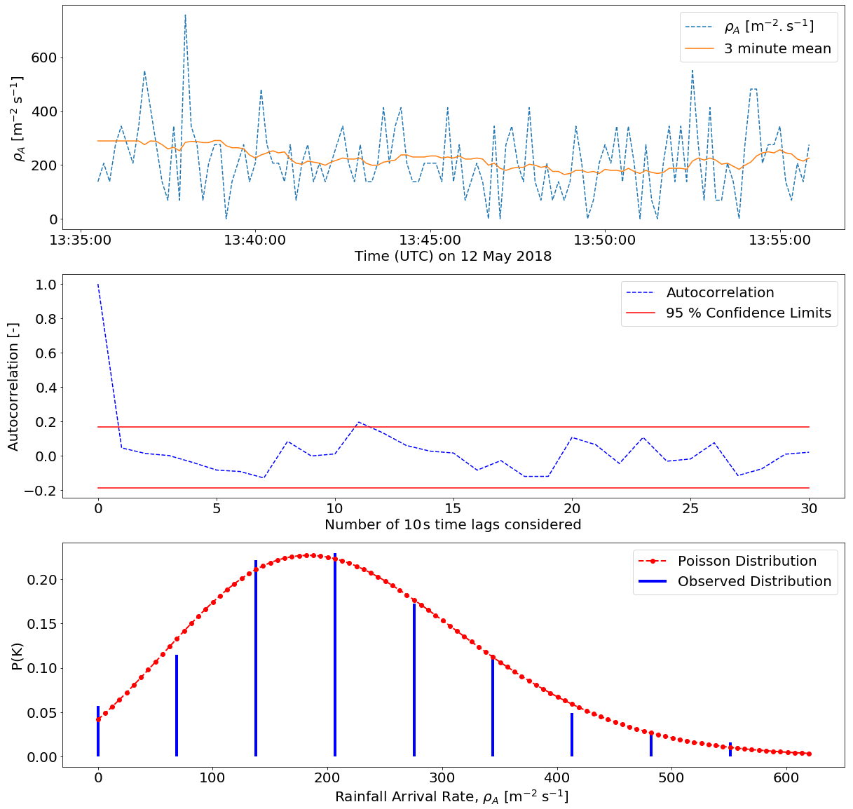
Figure 5A patch of rainfall, with a coherence time of 20 min, that can reasonably be assumed to be a sample of a Poisson process. The dispersion of the patch is 1.1 and the KL divergence is 0.01, indicating very good agreement between the observed PDF of the patch and the expected PDF from Poisson.
Tests 1 and 2 assess the stationarity and independence assumptions of a Poisson process. Test 3 checks that the distribution matches a Poisson distribution, and Tests 4 and 5 are quality checks. The quality checks are used because the sample size over which each test is conducted is often quite small. Figure 5 shows a good example of a patch of rainfall that passes all of the tests and can therefore reasonably be assumed to comply with the Poisson homogeneity hypothesis.
The rainfall rate is plotted in the top panel and can be characterised by uncorrelated fluctuations around a constant mean rate of arrival, in this case 220 . The corresponding PDF of this patch of rainfall along with the expected PDF of a Poisson process with the same mean arrival rate is plotted in the bottom panel. The auto-correlation function of the patch is plotted in the middle panel.
4.1 Rainfall rates
The total rainfall amounts [mm] measured by the co-located tipping bucket, intervalometer and disdrometer at the main site (Pole Pole) for the longest “online” period of the three instruments are presented in Fig. 6. Estimates of total rainfall are derived for both the disdrometer and intervalometer from the arrival rates using the three Marshall and Palmer (1948) type exponential parameterisations that were presented. For the disdrometer, the self-consistent Marshall and Palmer (1948) parameterisation underestimates the co-located tipping bucket rainfall amount by more than 50 %. The parameterisation with a fixed experimentally determined N0 underestimates the co-located tipping bucket rainfall amount by approximately 48 %. The power law parameterisation shows good agreement with the tipping bucket record and only underestimates the co-located tipping bucket rainfall amount by approximately 4 %. The results of the intervalometer are similar. The self-consistent Marshall and Palmer (1948) parameterisation underestimates the co-located tipping bucket rainfall amount by more than 70 %. The parameterisation with a fixed experimentally determined N0 underestimates the co-located tipping bucket rainfall amount by approximately 64 %. The power law parameterisation overestimates the co-located tipping bucket rainfall amount by approximately 12 %.
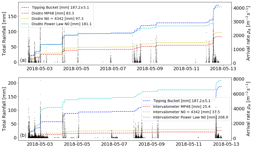
Figure 6The total rainfall amount [mm] observed by the co-located tipping bucket, intervalometer and disdrometer at the main site (Pole Pole) for the longest “online” period of the three instruments. Panel (a) compares the three DSD parameterisation estimates of rainfall to the observed tipping bucket rainfall amount for the disdrometer data. Panel (b) compares the three DSD parameterisation estimates of rainfall to the observed tipping bucket rainfall amount for the intervalometer data. Also plotted are the rainfall arrival rates measured by the disdrometer and intervalometer.
4.2 Testing the Poisson hypothesis
The coherence time or window length over which the Poisson tests were performed ranged from 2 to 22 min across all eight sites, with a typical length being in the order of 6 min. Using the tests defined in Sect. 3.4, we determined the rainfall patches that can reasonably be assumed to be representative of a Poisson process.
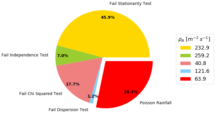
Figure 7The percentage of all rainfall patches, measured by the intervalometer, that fail each of the hierarchical tests as well as the mean rainfall arrival rate for each group. The presented data are an average, weighted by the length of each patch, across all of the intervalometer sites.
The proportion of rainfall patches, averaged across all the intervalometers, that do not conform with the Poisson hypothesis as well as the mean arrival rate for each group is presented in Fig. 7. Overall, 28.3 % of all patches can reasonably be assumed to be Poisson distributed. These are patches of stationary rainfall that exhibit no correlation between drop counts within a 95 % confidence interval, match a Poisson distribution very well and have a mean dispersion of approximately 1. The KL divergence of the Poisson patches was between 0.01 and 0.07 for all sites and only between 0 % and 7 % of all those patches had a KL divergence greater than 0.2.
Overall, 45.9 % of all patches failed the stationary tests and 7.0 % did not pass the independence test, indicating the presence of correlations between drop counts on scales as small as 2 min. It should be noted that these patches of rainfall are characterised by higher arrival rates (e.g. the rainfall that fails the independence test has a mean ρA that is approximately 4 times higher than the ρA of Poisson rain).
Of the remaining 47.1 % of rainfall patches, 17.7 % did not follow a Poisson distribution. Only a very small subset (1.2 %) did not pass the dispersion criteria and mostly because the observed variance was larger than expected for Poisson statistics. Again, these patches were characterised by higher raindrop arrival rates than the ones that passed.
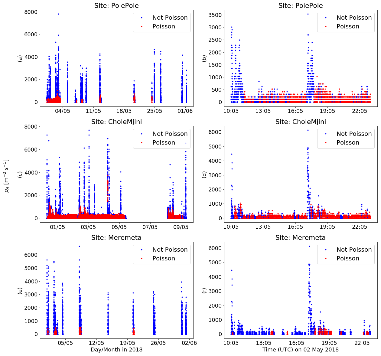
Figure 8The occurrence of Poisson rain in the rainfall records of three sites. The complete observational period is plotted in the left-hand column and a single large-scale storm which was common to all three sites is plotted in the right-hand column. The observational period in Meremeta and Pole Pole is much longer than that in Chole Mjini due to an instrument failure at that site.
Based on the previous results, it appears that most rainfall patches with higher raindrop arrival rates are inconsistent with the Poisson hypothesis. This can be clearly seen in the two middle panels (c, d) of Fig. 8 as well as panel (b). The time series in Fig. 8 clearly show that the mean rainfall arrival rate is a reasonable predictor of whether a given patch is likely to be Poisson or not. Figure 8 shows the total rainfall record for Pole Pole, Chole Mjini and Meremeta in the left-hand column and a single large-scale storm that was observed at all three sites in the right-hand column. This storm is characterised by sustained stratiform-type rainfall with low arrival rates and little fluctuation over time. This type of rainfall pattern is quite atypical for the rainfall record as a whole. Chole Mjini was only online for a relatively short period of time between 30 April and 8 May 2018, and this period happened to contain this atypical storm. The much longer time series for Pole Pole (panel a) and Meremeta (panel e) show that the observational record is dominated by intermittent rain events with sharp peaks and lots of convective rainfall followed by longer dry spells. Figure 8 also shows that most rainfall patches and in particular patches of rain with high rainfall arrival rates are typically not classified as Poisson, whereas many patches of rainfall with sustained low arrival rates (below 500 ) are classified as Poisson. This is especially evident in panels (b) and (d) where the two rainfall peaks do not pass the Poisson tests but the lower intensity patches in between them do.
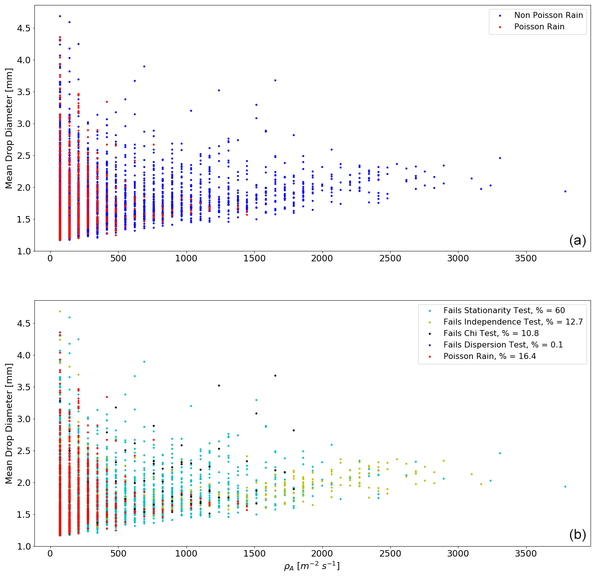
Figure 9Trends in mean drop size for Poisson and non-Poisson rain are presented as well as the percentage of drops that fail each of the Poisson tests. Panel (a) differentiates between Poisson and non-Poisson rain. Panel (b) is further subdivided to show which of the Poisson tests each data point fails.
The disdrometer drop size measurements can be used to characterise Poisson and non-Poisson rainfall patches further and are presented in Fig. 9. The mean drop size of each of the 10 s drop counts is plotted. The larger variance in mean drop size at lower arrival rates is due to the fact that these 10 s drop counts contain fewer drops, and therefore the mean is more susceptible to random sampling effects. The trend in mean drop size with rainfall arrival rate for Poisson and non-Poisson rain is presented in the top panel. It shows again that Poisson rain is characterised by low arrival rates. No examples of Poisson rain are found at ρA>1500 . The data also show a positive correlation between the mean drop sizes and the arrival rate.
The bottom panel of Fig. 9 presents, for each data point, the test that it fails. It shows that Poisson rain is found mostly at the lower end of the arrival rate range, ρA≤500 . This range of rainfall arrival rates contributes little to the total rainfall; 69 % of all drops fall in this range but only contribute 16 % to total rainfall. At arrival rates between 500 and 1300 , the rainfall is a mixture of Poisson rain and mostly patches of rainfall that fail the χ2 test. Data that fail the χ2 test are patches of stationary rainfall with uncorrelated fluctuations about the mean. However, the data are over- or underdispersed compared to the expected Poisson value of 1 and do not match the Poisson distribution. Mostly, these data are overdispersed; i.e. the variance is greater than expected by Poisson statistics. As arrival rate increases to between 1300 and 2000 , a higher proportion of rainfall (in this subrange) fails the stationarity and independence tests indicating that rainfall is becoming more and more dynamic (rapid changes in the mean and correlations between drop counts). At arrival rates greater than 2000 , the patches of rainfall predominantly fail the stationarity test. Arrival rates greater than 1000 systematically fail the independence tests and arrival rates greater than 2000 systematically fail the stationarity tests. This rainfall is characterised by correlations between drop counts and fluctuations in the mean arrival rate on scales of 2 to 22 min.
5.1 Rainfall rates
Three parameterisations of the DSD were presented. Of the three, the experimentally determined power law parameterisation resulted in the best estimates of the co-located tipping bucket rainfall amount for both the intervalometer (overestimate of 12 %) and the disdrometer (underestimate of 4 %). The other two parameterisations result in large underestimates of the total rainfall amount. The poor estimate of the total rainfall amount by these parameterisations is due to the poor agreement with the observed drop size distribution, in particular at larger drop sizes. These larger drop sizes contribute most to the rainfall amount. In the case of the self-consistent Marshall and Palmer (1948) parameterisation, the effect of truncation of the DSD also significantly contributes to the large underestimate of the rainfall amount. In Fig. 4, the three parameterisations are plotted against the observed drop sizes for the entire observational period. The parameterisation with a fixed value of N0 determined from the entire observational period fits the observed data best. This is because it was derived from the data. However, whilst the agreement with the observed data is best overall, it underestimates the larger drop sizes of D>2.5 mm. The self-consistent Marshall and Palmer (1948) parameterisation shows the poorest fit with the observed data and also results in the worst rainfall estimates. The self-consistent Marshall and Palmer (1948) parameterisation overestimates small drop sizes and largely underestimates larger drop sizes. The experimentally determined power law parameterisation underestimates smaller drop sizes but correctly estimates larger drop sizes and overestimates very large drop sizes. Since the larger drops contribute most to the rainfall amount, the parameterisation which models this part of the DSD best, which is the N0 power law parameterisation, results in the best rainfall rate estimates. These results clearly show the importance of accurately modelling the DSD, particularly at larger drop sizes, for rainfall estimation.
The intervalometer and disdrometer had different sensors. The intervalometer has a smaller minimum detectable drop size than the disdrometer (0.8 and 1 mm, respectively). This can be clearly seen in Fig. 6, where the intervalometer registers higher arrival rates than the disdrometer for every observed rainfall event. The different minimum detectable drop sizes for each instrument indicate that they observe different DSDs. Therefore, parameterisations derived from the disdrometer are not optimal for use with the intervalometer. Despite this challenge, the estimate of the rainfall amount by the power law is quite reasonable and shows promise for the intervalometer concept. Furthermore, the estimate of rainfall amount using the disdrometer measurements by the N0 power law parameterisation shows excellent agreement with the co-located tipping bucket. Note that this estimate was derived by using the disdrometer in intervalometer mode; i.e. only the drop counts were used to estimate rainfall amount. These results show the potential for using intervalometers to measure rainfall; however, they also highlight the need for proper calibration of the DSD model using data from a similarly sensitive instrument from the local climate that the intervalometer will be placed in.
5.2 Testing the Poisson hypothesis
The results of the hierarchical tests show that the majority of rainfall tested does not comply with the Poisson homogeneity hypothesis. This is because the rainfall record is dominated by dynamic convective storms that are characterised by high arrival rates that are fluctuating on very short timescales (<2 min in some cases). This rainfall is also characterised by correlations between drop counts on these timescales. This convective-type rainfall, which contributes most to the total rainfall amount (>80 %) in this study, is almost never classified as Poisson and does not exhibit characteristics that are consistent with Poisson statistics.
Another type of rainfall is also observed in the rainfall record. This stratiform-type rain is characterised by sustained periods of consistent low-intensity rainfall that has few fluctuations in the mean arrival rate. Rainfall of this type is often classified as Poisson and appears to exhibit characteristics that are consistent with Poisson statistics, yet it contributes less than a fifth to the total rainfall amount.
How do we explain the fact that rainfall estimates based on a parameterisation which has been defined independently of a notion of scale, and therefore implies homogeneity, are quite good for both the disdrometer and intervalometer arrival rates? At the same time, the majority of rainfall does not comply with the Poisson hypothesis. Is something fishy going on?
The regime of tests implemented in this study aims to assess the validity of the Poisson hypothesis in rainfall estimation. That is, the tests are binary (yes vs. no) in nature. We find that for most of the rainfall the Poisson hypothesis is not strictly true. However, the usefulness of the Poisson hypothesis is not tested. This approach may be too short-sighted and other, more practically oriented diagnostic tools could be designed to determine the conditions under which the Poisson hypothesis is likely to result in good estimates of rainfall rates (or drop diameters). So, whilst the Poisson model may not be strictly true for the rainfall observed in this study, it does appear to be a good approximation and highly useful for estimating rainfall rates.
There is also the issue that the regime of tests used in this study is likely biased such that rainfall with lower arrival rates is much more likely to be classified as Poisson than rainfall with higher arrival rates. This is due to inherent differences between low and high rainfall arrival rates and also the failure of the χ2 goodness-of-fit test to reject the null hypothesis at small sample sizes. The majority of low-arrival-rate rainfall generally occurs in patches of rainfall characterised by reasonably stationary mean arrival rate and uncorrelated fluctuations around this mean. High arrival rates occur in highly dynamic patches of rainfall that have changes in the mean at smaller timescales than most of the patches tested in this study. Consequently, almost no rainfall with high arrival rates passes the stationarity and independence tests, whereas a very large proportion of rainfall with low arrival rates does. The χ2 goodness-of-fit test is then conducted almost exclusively on patches of rainfall with low arrival rates. These patches have small sample sizes, and the power of the χ2 test to reject the null hypothesis is limited at these sample sizes.
This is well understood in statistics and has led to various sampling criteria, such as a minimum of five observations per rainfall arrival rate class for the χ2 goodness-of-fit test (Conover, 1999). This criterion is not used in this study. However, as pointed out by Kostinski and Jameson (1997), Jameson and Kostinski (1998), Kostinski et al. (2006) and Kostinski and Jameson (2000), rainfall conditions are changing rapidly, sometimes on temporal scales smaller than 2 min. The presence of these fine structures within rainfall would be obscured by larger sampling windows. Furthermore, sampling across such structures with different means may actually lead to increased uncertainty in the mean. Kostinski et al. (2006) noted that on the temporal resolution, some experiments will pick up the super-Poissonian variance and some will not. Similarly, at longer timescales, the auto-correlation can no longer be calculated, making it hard to define patches on which the Poisson assumptions can be tested. This increased uncertainty in the mean over an entire rainfall event would make it almost impossible to test the homogeneous Poisson hypothesis because rainfall is very rarely stationary over longer time periods.
The high acceptance rate of the Poisson hypothesis at low arrival rates observed in this study may be driven by the failure of the statistical tests to reject the null hypothesis at low sample sizes. However, despite the presence of spurious patches of Poisson rainfall, there are also many examples of patches that are likely to be genuine representations of the Poisson distribution, such as in Fig. 5. It is difficult to differentiate between these patches with the statistical tests given the small sample sizes. It is also not clear whether these genuine Poisson patches occur because the homogeneous Poisson hypothesis is applicable under certain rainfall conditions, e.g. consistent light stratiform-type rainfall, or whether these patches arise through randomness due to the sheer number of rainfall patches tested. This should be investigated further.
These findings highlight some limitations in how rainfall is observed with ground-based instruments. The intervalometer and disdrometer used in this study had a surface area of 9.6 and 14.5 cm2, respectively. Consequently, the number of drops that is observed is quite low, and the number of 10 s drop counts for a coherence time of 2 min is only 12. Practically, this means that statistical tests do not have enough power to reject the null hypothesis. Furthermore, increasing the length of the coherence time is not a suitable solution. The presence of these fine structures within rainfall would be obscured by larger sampling windows.
New sampling techniques or observation methodologies are needed to increase the effective sample size. One way of increasing the number of available observations is by increasing the effective surface area of the measuring instruments. This can be done by using many co-located instruments. In this way, the number of observations per window of time could be increased and the aggregation bin could be decreased to 5 or 1 s, thus increasing the number of drop counts available for testing at very short patch lengths. The number of observations could also be increased by increasing the sensitivity of the sensors to lower drop diameters. Another possibility would be to use adaptive sampling techniques, i.e. make sure each time interval has the same number of raindrops or rainfall amount, similarly to the idea proposed by Schleiss (2017). This would allow for a better interrogation of the Poisson hypothesis on the very fine rainfall structures present in convective storms.
Despite the issue with sample size and the fact that the Poisson hypothesis is likely not strictly true, the presence of significant amounts of homogeneous Poisson rain combined with the accuracy of derived rainfall estimates found in this study is compelling evidence for retaining the Poisson model. Furthermore, as was pointed out by Jameson and Kostinski (1998), the observed presence of any non-clustering Poissonian structures in the rainfall conflicts with a fractal description of rain and is a good argument against abandoning the Poisson framework completely for a fractal description or some other model.
This research leads to the following conclusions:
-
The majority of rainfall and almost all the convective-type rainfall, which contributed most to total rainfall amount in this study, did not exhibit characteristics that are consistent with the Poisson hypothesis. Patches that complied with the Poisson hypothesis were characterised by low mean rainfall arrival rates during periods of sustained stratiform-type rainfall. No examples of Poisson-distributed rain patches, with ρA>1500 , were observed. Changes in the mean drop arrival rate and correlations between drop counts at scales as small as 2 min accounted for deviations from Poisson in 52.9 % of all rainfall patches.
-
There appear to be genuine examples of Poisson rainfall that occur during consistent light stratiform-type rainfall conditions. However, small sample sizes were an issue in this study and may have resulted in the statistical tests failing to reject the null hypothesis of Poisson at low arrival rates for many rainfall patches, making it hard to differentiate between genuine and spurious Poisson rainfall. Increasing the patch length is not a suitable solution to increase the number of observations. Fine structures are observed in rainfall at very small scales, and sampling across such structures with different means may actually lead to increased uncertainty in the mean. New sampling techniques or observation methodologies are needed to increase the effective sample size.
-
Total cumulative rainfall estimates derived from the disdrometer drop counts with the best-performing Marshall and Palmer (1948) type parameterisation (power law of N0) were within 4 % of co-located tipping bucket measurements.
-
Total cumulative rainfall estimates derived from the best-performing Marshall and Palmer (1948) type parameterisation (power law of N0) resulted in an overestimate of almost 12 %. This was most likely due to model error since the parameterisations were derived for the disdrometer. The accuracy of rainfall estimates is largely determined by the validity of the DSD parameterisation as well as the accuracy of the sensor.
-
It is possible to retrieve rainfall rates using an intervalometer. The intervalometer principle shows potential for providing ground-based rainfall observations in remote areas of Africa. The main advantage of this instrument is its low cost. However, further improvements are needed to make the sensor more robust, as several instruments were damaged by water during this study. The results also show that it is necessary to verify the DSD model with observed drop size data from within the local climate with an instrument that has the same sensitivity as the intervalometer.
Data and corresponding Python scripts for analysis are available from the corresponding author upon request.
RH and NvdG contributed to the designs of the disdrometer and intervalometer. NvdG and MCtV were responsible for acquiring funding. DdV and NvdG designed the experiment. Data were collected by DdV. Analysis was performed by DdV, with contributions from NvdG, MCtV and MS. DdV prepared the draft of the manuscript with contributions from all the co-authors.
The authors declare that they have no conflict of interest.
The opinions expressed in the document are of the authors
only and no way reflect the European Commission's opinions. The European
Union is not liable for any use that may be made of the information.
Publisher's note: Copernicus Publications remains neutral with regard to jurisdictional claims in published maps and institutional affiliations.
The following are acknowledged (in no particular order) for their work in developing the disdrometer and intervalometer: Stijn de Jong, Jan Jaap Pape, Coen Degen, Ravi Bagree, Jeroen Netten, Els Veenhoven, Dirk van der Lubbe-Sanjuan, Wouter Berghuis, Rolf Hut and Nick van de Giesen. Special thanks are given to the hotels located on Mafia Island (Didimiza Guest House, Meremeta Lodge, Eco Shamba Kilole Lodge, Kinasi Lodge, Pole Pole Bungalows and the Mafia Island Lodge) and Chole Island (Chole Mjini Treehouse Lodge) for allowing access to their land and providing support in setting up the experiment.
This research has been supported by the European Community's Horizon 2020 Programme (grant no. 776691).
This paper was edited by Piet Stammes and reviewed by Remko Uijlenhoet and two anonymous referees.
Abdrabo, M., Essel, A., Lennard, C., Padgham, J., and Urquhart, P.: Africa, in: Climate Change 2014: Impacts, Adaptation, and Vulnerability. Part B: Regional Aspects. Contribution of Working Group II to the Fifth Assessment Report of the Intergovernmental Panel on Climate Change, Tech. rep., Cambridge University Press, Cambridge, UK and New York, NY, USA, 2014. a
Arfken, G. B., Weber, H. J., and Harris, F. E.: Mathematical Methods for Physicists, 7th edn., Academic Press, Cambridge, Massachusetts, USA, 2013. a
Atlas, D. and Ulbrich, C. W.: Path- and Area-Integrated Rainfall Measurement by Microwave Attenuation in the 1–3 cm Band, J. Appl. Meteorol., 16, 1322–1331, https://doi.org/10.1175/1520-0450(1977)016<1322:paairm>2.0.co;2, 1977. a, b, c, d
Battan, L. J.: Radar Observation of the Atmosphere, University of Chicago Press, Chicago, Illinois, USA, 1973. a
Boko, M., Niang, I., and Nyong, A.: Africa, in: Climate change adaptation and vulnerability: contribution of working group II to the IV assessment report of the IPCC panel on climate change, Tech. rep., Cambridge University Press, Cambridge, UK and New York, NY, USA, 2007. a
Bringi, V. N., Chandrasekhar, V., Hubbert, J., Gorgucci, E., Randeu, W. L., and Schoenhuber, M.: Raindrop size distribution in different climatic regimes from disdrometer and dual-polarized radar analysis, J. Atmos. Sci., 60, 354–365, 2003. a
Ciach, G. J.: Local Random Errors in Tipping-Bucket Rain Gauge Measurements, J. Atmos. Ocean. Tech., 25, 752–759, https://doi.org/10.1175/1520-0426(2003)20<752:LREITB>2.0.CO;2, 2003. a
Conover, W. J.: Practical Nonparametric Statistics, 3rd edn., John Wiley and Sons, Hoboken, New Jersey, USA, 1999. a
Cox, D. and Isham, V.: Point Processes, Chapman and Hall, London, UK, 1980. a
Dickey, D. A. and Fuller, W. A.: Distribution of the Estimators for Autoregressive Time Series with a Unit Root, J. Am. Stat. Assoc., 74, 423–431, 1979. a, b
Feingold, G. and Levin, Z.: The Lognormal Fit to Raindrop Spectra from Frontal Convective Clouds in Israel, J. Clim. Appl. Meteorol., 25, 1346–1363, https://doi.org/10.1175/1520-0450(1986)025<1346:tlftrs>2.0.co;2, 1986. a, b
Feller, W.: An Introduction to Probability Theory and its Applications, Wiley, Hoboken, New Jersey, USA, 2010. a
Greatrex, H., Hansen, J., Garvin, S., Diro, R., Blakeley, S., Le Guen, M., Rao, K., and Osgood, D.: Scaling up index insurance for smallholder farmers: Recent evidence and insights, Tech. Rep. 14, CGIAR Research Program on Climate Change, Agriculture and Food Security (CCAFS), Copenhagen, Denmark, 2015. a
Greene, W. H.: Econometric Analysis, 5th edn., Pearson, New York City, New York, USA, 2003. a
Gunn, R. and Kinzer, G. D.: The Terminal Velocity Of Fall For Water Droplets In Stagnant Air, J. Meteorol., 6, 243–248, https://doi.org/10.1175/1520-0469(1949)006<0243:ttvoff>2.0.co;2, 1949. a
Guyot, A., Pudashine, J., Protat, A., Uijlenhoet, R., Pauwels, V. R. N., Seed, A., and Walker, J. P.: Effect of disdrometer type on rain drop size distribution characterisation: a new dataset for south-eastern Australia, Hydrol. Earth Syst. Sci., 23, 4737–4761, https://doi.org/10.5194/hess-23-4737-2019, 2019. a, b
Haan, C.: Statistical Methods in Hydrology, The Iowa State University Press, Iowa City, Iowa, USA, 1977. a
Hershey, J. R. and Olsen, P. A.: Approximating the Kullback Leibler Divergence Between Gaussian Mixture Models, Institute of Electrical and Electronic Engineers, https://doi.org/10.1109/ICASSP.2007.366913, 2007. a
Hosking, J. G. and Stow, C. D.: The Arrival Rate of Raindrops at the Ground, J. Appl. Meteorol. Clim., 26, 433–442, https://doi.org/10.1175/1520-0450(1987)026<0433:TARORA>2.0.CO;2, 1987. a
Humphrey, M. D., Istok, J. D., Lee, J. Y., Hevesi, J. A., and Flint, A. L.: A New Method for Automated Dynamic Calibration of Tipping-Bucket Rain Gauges, J. Atmos. Ocean. Tech., 14, 1513–1519, https://doi.org/10.1175/1520-0426(1997)014<1513:ANMFAD>2.0.CO;2, 1997. a
Hut, R.: New Observational Tools and Datasources for Hydrology: Hydrological data Unlocked by Tinkering, PhD thesis, Delft University of Technology, https://doi.org/10.4233/uuid:48d09fb4-4aba-4161-852d-adf0be352227, 2013. a
Iguchi, T., Seto, S., Meneghini, R., Yoshida, N., Awaka, J., Le, M., Chandrasekar, V., and Kubota, T.: GPM/DPR Level-2 Algorithm Theoretical Basis Document, Tech. rep., NASA, Washington, D.C., USA, available at: https://gpm.nasa.gov/resources/documents/gpmdpr-level-2-algorithm-theoretical-basis-document-atbd (last access: 17 August 2021), 2017. a, b
Jameson, A. R. and Kostinski, A. B.: Fluctuation Properties of Precipitation. Part II: Reconsideration of the Meaning and Measurement of Raindrop Size Distributions, J. Atmos. Sci., 55, 283–294, https://doi.org/10.1175/1520-0469(1998)055<0283:fpoppi>2.0.co;2, 1998. a, b, c
Johnson, R. W., Kliche, D. V., and Smith, P. L.: Comparison of Estimators for Parameters of Gamma Distributions with Left-Truncated Samples, J. Appl. Meteorol. Clim., 50, 296–310, https://doi.org/10.1175/2010jamc2478.1, 2011. a
Joss, J. and Waldvogel, A.: Raindrop Size Distribution and Sampling Size Errors, J. Atmos. Sci., 26, 566–569, https://doi.org/10.1175/1520-0469(1969)026<0566:rsdass>2.0.co;2, 1969. a
Kostinski, A. and Jameson, A.: On the Spatial Distribution of Cloud Particles, J. Atmos. Sci., 57, 901–915, https://doi.org/10.1175/1520-0469(2000)057<0901:OTSDOC>2.0.CO;2, 2000. a
Kostinski, A., Larsen, M., and Jameson, A.: The texture of rain: Exploring stochastic micro-structure at small scale, J. Hydrol., 328, 38–45, https://doi.org/10.1016/j.jhydrol.2005.11.035, 2006. a, b
Kostinski, A. B. and Jameson, A. R.: Fluctuation Properties of Precipitation. Part I: On Deviations of Single-Size Drop Counts from the Poisson Distribution, J. Atmos. Sci., 54, 2174–2186, https://doi.org/10.1175/1520-0469(1997)054<2174:fpoppi>2.0.co;2, 1997. a, b, c, d, e, f, g
Kullback, S.: Information Theory and Statistics, Dover Publications, Mineola, New York, USA, 1968. a
Kwiatkowski, D., Phillips, P., Schmidt, P., and Shin, Y.: Testing the Null Hypothesis of Stationarity Against the Alternative of a Unit Root: How Sure Are we that Economic Time Series Have a Unit root?, J. Econometrics, 54, 159–178, 1992. a, b
Lavergnat, J. and Golé, P.: A Stochastic Raindrop Time Distribution Model, J. Appl. Meteorol., 37, 805–818, https://doi.org/10.1175/1520-0450(1998)037<0805:asrtdm>2.0.co;2, 1998. a
Lovejoy, S. and Schertzer, D.: Fractals, Raindrops and Resolution Dependence of Rain Measurements, J. Appl. Meteorol., 29, 1167–1170, https://doi.org/10.1175/1520-0450(1990)029<1167:frardo>2.0.co;2, 1990. a
Maity, R.: Statistical Methods in Hydrology and Hydroclimatology, Springer, New York City, New York, USA, 2018. a
Marshall, J. S. and Palmer, W. M.: The distribution of raindrops with size, J. Meteorol., 5, 165–166, 1948. a, b, c, d, e, f, g, h, i, j, k, l, m, n, o, p, q, r, s, t, u
Munchak, S. J. and Tokay, A.: Retrieval of Raindrop Size Distribution from Simulated Dual-Frequency Radar Measurements, J. Appl. Meteorol. Clim., 47, 223–239, https://doi.org/10.1175/2007jamc1524.1, 2008. a, b
Otto, F. E. L., Boyd, E., Jones, R. G., Cornforth, R. J., James, R., Parker, H. R., and Allen, M. R.: Attribution of extreme weather events in Africa: a preliminary exploration of the science and policy implications, Climatic Change, 132, 531–543, https://doi.org/10.1007/s10584-015-1432-0, 2015. a
Pearson, K. F. R. S.: On the criterion that a given system of deviations from the probable in the case of a correlated system of variables is such that it can be reasonably supposed to have arisen from random sampling, The London, Edinburgh, and Dublin Philosophical Magazine and Journal of Science, 50, 157–175, 1900. a
Schleiss, M.: Scaling and Distributional Properties of Precipitation Interamount Times, J. Hydrometeorol., 18, 1167–1184, https://doi.org/10.1175/JHM-D-16-0221.1, 2017. a
Schwert, G. W.: Tests for unit roots: A Monte Carlo investigation, J. Bus. Econ. Stat., 50, 5–17, https://doi.org/10.1198/073500102753410354, 2012. a
Smith, J. A.: Marked Point Process Models of Raindrop-Size Distributions, J. Appl. Meteorol., 32, 284–296, https://doi.org/10.1175/1520-0450(1993)032<0284:mppmor>2.0.co;2, 1993. a, b
Tokay, A. and Short, D. A.: Evidence from Tropical Raindrop Spectra of the Origin of Rain from Stratiform versus Convective Clouds, J. Appl. Meteorol., 35, 355–371, https://doi.org/10.1175/1520-0450(1996)035<0355:eftrso>2.0.co;2, 1996. a, b
Tokay, A., Kruger, A., and Krajewski, W. F.: Comparison of Drop Size Distribution Measurements by Impact and Optical Disdrometers, J. Appl. Meteorol., 40, 2083–2097, https://doi.org/10.1175/1520-0450(2001)040<2083:codsdm>2.0.co;2, 2001. a
Uijlenhoet, R. and Stricker, J. N. M.: A consistent rainfall parameterization based on the exponential drop size distribution, J. Hydrol., 218, 101–127, 1999. a, b, c, d, e
Uijlenhoet, R., Stricker, J., Torfs, P., and Creutin, J.-D.: Towards a stochastic model of rainfall for radar hydrology: testing the poisson homogeneity hypothesis, Phys. Chem. Earth Pt. B, 24, 747–755, https://doi.org/10.1016/s1464-1909(99)00076-3, 1999. a, b, c
Ulbrich, C. W.: Natural Variations in the Analytical Form of the Raindrop Size Distribution, J. Clim. Appl. Meteorol., 22, 1764–1775, 1983. a, b
Ulbrich, C. W.: The Effects of Drop Size Distribution Truncation on Rainfall Integral Parameters and Empirical Relations, J. Appl. Meteorol. Clim., 24, 580–590, https://doi.org/10.1175/1520-0450(1985)024<0580:TEODSD>2.0.CO;2, 1985. a, b, c
Waldvogel, A.: The N0 Jump of Raindrop Spectra, J. Atmos. Sci., 31, 1067–1078, https://doi.org/10.1175/1520-0469(1974)031<1067:TJORS>2.0.CO;2, 1974. a
Wang, W., Vrijling, J. K., Van Gelder, P. H. A. J. M., and Ma, J.: Testing for nonlinearity of streamflow processes at different timescales, J. Hydrol., 322, 247–268, 2006. a, b
Washington, R., Harrison, M., Conway, D., Black, E., Challinor, A., Grimes, D., Jones, R., Morse, A., Kay, G., and Todd, M.: African Climate Change: Taking the Shorter Route, B. Am. Meteorol. Soc., 87, 1355–1366, https://doi.org/10.1175/BAMS-87-10-1355, 2006. a