A simulation-experiment-based assessment of retrievals of above-cloud temperature and water vapor using a hyperspectral infrared sounder

Measuring atmospheric conditions above convective storms using spaceborne instruments is challenging. The operational retrieval framework of current hyperspectral infrared sounders adopts a cloud-clearing scheme that is unreliable in overcast conditions. To overcome this issue, previous studies have developed an optimal estimation method that retrieves the temperature and humidity above high thick clouds by assuming a slab of cloud. In this study, we find that variations in the effective radius and density of cloud ice near the tops of convective clouds lead to non-negligible spectral uncertainties in simulated infrared radiance spectra. These uncertainties cannot be fully eliminated by the slab-cloud assumption. To address this problem, a synergistic retrieval method is developed here. This method retrieves temperature, water vapor, and cloud properties simultaneously by incorporating observations from active sensors in synergy with infrared radiance spectra. A simulation experiment is conducted to evaluate the performance of different retrieval strategies using synthetic radiance data from the Atmospheric Infrared Sounder (AIRS) and cloud data from CloudSat/CALIPSO. In this experiment, we simulate infrared radiance spectra from convective storms through a combination of a numerical weather prediction model and a radiative transfer model. The simulation experiment shows that the synergistic method is advantageous, as it shows high retrieval sensitivity to the temperature and ice water content near the cloud top. The synergistic method more than halves the root-mean-square errors in temperature and column integrated water vapor compared to prior knowledge based on the climatology. It can also improve the quantification of the ice water content and effective radius compared to prior knowledge based on retrievals from active sensors. Our results suggest that existing infrared hyperspectral sounders can detect the spatial distributions of temperature and humidity anomalies above convective storms.

1 Introduction

Water vapor in the upper troposphere and lower stratosphere (UTLS) plays an essential role in the Earth's climate system due to its important radiative effects (Huang et al., 2010; Dessler et al., 2013) and chemical effects (Shindell, 2001; Kirk-Davidoff et al., 1999; Anderson et al., 2012).

Our understanding of UTLS water vapor has long been informed by accurate in situ observations carried out during aircraft and balloon campaigns. Long-term records provided by balloon-borne observations have suggested a decadal increase in stratospheric water vapor (Oltmans et al., 2000; Rosenlof et al., 2001; Hurst et al., 2011) but a decadal cooling in tropical tropopause temperature over the same period (Rosenlof et al., 2001; Randel et al., 2004). These contradictory trends in water vapor and temperature are not reproduced well by reanalysis products (Davis et al., 2017), and the key processes at play are still under debate. This increase in UTLS water vapor, if true, may accelerate the decadal rate of surface warming through its impact on thermal radiation (Solomon et al., 2010). While balloon-borne instruments suggest possible changes in UTLS water vapor, aircraft campaigns reveal that UTLS water vapor can be highly variable under the influence of deep convection. By sampling plumes from convective detrainment, these campaigns have found that overshooting deep convection can increase the UTLS water vapor by injecting moist plumes or ice particles that sublimate in a warmer environment (e.g., Corti et al., 2008; Schiller et al., 2009; Anderson et al., 2012; Sun and Huang, 2015; Smith et al., 2017). Despite substantial evidence of convective hydration, it has been argued that the overall impact of convection on the global UTLS water vapor budget might be negligible (e.g., Ueyama et al., 2018; Schoeberl et al., 2019; Randel and Park, 2019).

Therefore, long-term global observations of UTLS water vapor, especially above convective storms, are essential. However, the operational global radiosonde network does not perform well in cold and low-pressure environments such as the UTLS (Kley, 2000). Moreover, while satellite observational products have been extensively used to investigate the spatial and temporal variability of UTLS water vapor (Sun and Huang, 2015; Randel and Park, 2019; Yu et al., 2020; Wang and Jiang, 2019; Jiang et al., 2020), these products have some limitations. Although limb-viewing and solar occultation instruments are sensitive to the UTLS region, they are not suitable for detecting small-scale variability above convective storms because the horizontal sampling footprints of these instruments are larger than 100 km. Furthermore, contamination from convective clouds leads to higher uncertainty in the current products of microwave sounders (such as MLSv4.2, Livesey et al., 2017) due to strong scattering. Moreover, because they are limited by the occurrence of solar occultation, instruments that use this technique do not provide sufficient sampling to study convective events.

Meanwhile, the current hyperspectral sounding framework of the NOAA and NASA adopts a cloud-clearing scheme (Susskind et al., 2003; Gambacorta et al., 2014). This scheme infers the radiance of clear scenes from a 3 × 3 set of adjacent instrument fields of view (FOVs) with different cloud amounts, assuming the same temperature and atmospheric absorber (including water vapor) fields in all FOV footprints (∼ 13.5 km). Consequently, such a cloud-clearing scheme fails in overcast cloud conditions (i.e., when there are the same cloud amounts in adjacent footprints) or when thermodynamic properties vary drastically among adjacent footprints. For this reason, the current retrieval products from hyperspectral infrared sounders, including AIRS (the Atmospheric Infrared Sounder; Chahine et al., 2006), IASI (Infrared Atmospheric Sounding Interferometer; Blumstein et al., 2004), and CrIS (Cross-track Infrared Sounder; Bloom, 2001), are not reliable above convective storms.

Recently, researchers have demonstrated the feasibility of performing single-footprint retrievals in cloudy-sky conditions from AIRS using an optimal estimation (OE) scheme (DeSouza-Machado et al., 2018; Irion et al., 2018; Feng and Huang, 2018). Using the same instrument, such single-footprint retrievals improve the spatial resolution from 40.5 km in the cloud-clearing scheme to 13.5 km. In those studies, DeSouza-Machado et al. (2018) used the a priori cloud state from a numerical weather prediction (NWP) model and then adjusted the cloud state to match the observed brightness temperature of an infrared window channel. Irion et al. (2018) retrieved the cloud optical depth, cloud effective radius, and the cloud-top temperature by obtaining a priori data from collocated MODIS (Moderate Resolution Imaging Spectroradiometer; Platnick et al., 2003) observations. While DeSouza-Machado et al. (2018) and Irion et al. (2018) discussed the implementation of an all-sky, single-footprint OE scheme in general, Feng and Huang (2018) focused especially on optically thick cloud conditions, for which they conducted a comprehensive information content analysis. They showed that existing hyperspectral infrared sounders present substantial numbers of degrees of freedom for signal (DFS; a higher DFS indicates greater vertical resolution) in UTLS temperature (∼ 5) and water vapor (∼ 1). They also found that the presence of thick cloud in the upper troposphere increases the DFS compared to clear-sky conditions. By validating the retrieval using in situ observations carried by aircraft campaigns, Feng and Huang (2018) demonstrated that it is possible to detect both hydration and dehydration anomalies in the UTLS using current infrared hyperspectral sounders. In the case of optically thick clouds, e.g., deep convective clouds, these studies (DeSouza-Machado et al., 2018; Irion et al., 2018; Feng and Huang, 2018) similarly represent the cloud as a slab (an optically thick and uniform layer) of ice clouds with fixed microphysical properties, based on cloud states inferred a priori from the brightness temperature of an infrared window channel, NWP, or coincident passive cloud instrument (e.g., MODIS). Retrieval methods that use this cloud assumption are referred to as slab-cloud methods hereafter.

However, neglecting the variability in cloud mass and microphysical properties leads to uncertainty in the thermal emission of the cloud, and this emission greatly contributes to the observed top-of-atmosphere (TOA) radiances. Yang et al. (2013) showed that the scattering and absorption properties of ice clouds across the infrared spectrum are greatly impacted by the size and shape of ice particles. Furthermore, deep convective clouds are typically associated with large temperature perturbations near the cloud top and drastic temperature decreases with altitude (Biondi et al., 2012). If there is an anomalous temperature field, inferring the cloud-top position from the brightness temperature of an infrared window channel, as done in previous studies, can lead to biases (Sherwood et al., 2004). When the temperature lapse rate is large, the vertical distribution of ice content can influence the thermal emission of the cloud. Therefore, it is necessary to assess and constrain the impacts of these factors on the retrieval accuracy.

These uncertainties regarding clouds can be reduced by combining collocated observations from active sensors onboard the same satellite constellation. The A-Train satellite constellation uniquely provides collocated observations from an orbital hyperspectral infrared sounder (i.e., AIRS) and active remote-sensing instruments, including the cloud profiling radar aboard CloudSat (Stephens et al., 2008) and CALIOP (Cloud–Aerosol Lidar with Orthogonal Polarization) aboard CALIPSO (Cloud-Aerosol Lidar and Infrared Pathfinder Satellite Observation; Winker et al., 2010). Before the year 2015, these instruments passed over nearly the same locations within 2 min of each other while traveling along the A-Train orbit track. The nearest lidar (90 m × 90 m) and CPR (2.5 km × 1.4 km) footprints were typically located around 5 km from the center of the AIRS footprints (13.5 km × 13.5 km), well within the AIRS FOVs.

DARDAR-Cloud (Delanoë and Hogan, 2008, 2010) is a joint product that combines radar reflectivity measurements from CPR with the lidar attenuated backscatter ratio from CALIOP to provide ice water content (IWC) and effective radius profiles at each CPR footprint. Compared to passive instruments, this joint product is more sensitive to the vertical ice distribution near the cloud top, which can be an important influence on the thermal emission of the cloud. In the present work, we develop an optimal estimation method to retrieve the temperature, water vapor, ice water content, and effective radius simultaneously by incorporating active cloud remote-sensing products and infrared hyperspectra, using the DARDAR-Cloud product and AIRS L1B observations to construct an example. A retrieval method that incorporates such collocated cloud products is referred to as a synergistic method.

In this paper, we first quantify the uncertainty in infrared radiance spectra induced by cloud optical properties. We then evaluate the performance of retrieval strategies that use the slab-cloud and synergistic methods following a simulation experiment emulating an implementation based on the AIRS L1B and DARDAR-Cloud products. This experiment simulates observational signals from realistic temperature, humidity, and cloud fields above a deep convective event simulated by an NWP model. Section 2 describes the main components of this simulation experiment. We then implement different retrieval strategies, as formulated in Sect. 2.3, to retrieve from synthetic observations. The results are evaluated in Sect. 3 by comparing the retrievals to the prescribed truth. The application of the improved synergistic retrieval scheme to existing instruments is discussed in Sect. 4.

2 Method

The simulation experiment in this study consists of the following components:

1. a cloud-resolving NWP model that is used to provide the true atmospheric conditions (the “truth”) during a tropical cyclone event and to construct a priori and test sets, as described in Sect. 2.1;

2. a radiative transfer model that is used to generate synthetic observations with the AIRS instrument specifications and as the forward model in the retrieval, as described in Sect. 2.2;

3. retrieval algorithms, as explained in Sect. 2.3; and

4. comparisons between the retrieved quantities and the NWP-generated truth in Sect. 3.

A tropical cyclone event is simulated because it generates a vast convective cloud system that covers a large spatial domain for contrasting the above-storm temperature and humidity fields. In the framework of this simulation experiment, we neglect the complexity of the scan geometry of the instrument by assuming that the instrument views from the nadir, that the atmospheric conditions are uniform within one footprint, and that coincident cloud products are available for every sample. In reality, the scanning angle of AIRS footprints for which the nearest CloudSat footprints are within 6.5 km from the center is around 16^∘ off the nadir.

2.1 Numerical weather prediction model

In this study, we use the Global Environmental Multiscale (GEM) model of Environment and Climate Change Canada (hereafter ECCC; Côté et al., 1998; Girard et al., 2014) to provide a detailed and realistic representation of storm-impacted atmospheric and cloud profiles, following the study by Qu et al. (2020). The GEM model is formulated using nonhydrostatic primitive equations with a terrain-following hybrid vertical grid. It can be run as a global model or a limited-area model and is capable of one-way self-nesting. For the experiments conducted here, three self-nested domains are used with areas of 3300 × 3300, 2000 × 2000, and 1024 × 1024 km² and horizontal grid spacings of 10, 2.5, and 1 km, respectively, centered at 141^∘ E, 16^∘ N. All simulations use 67 vertical levels, with a vertical grid spacing Δz ∼ 250 m in the UTLS region and the model top at 13.5 hPa (29.1 km). The simulation is initialized with conditions from the ECCC global atmospheric analysis at 00:00 UTC 16 May 2015. It runs for 24 h until 00:00 UTC on 17 May 2015. A model spin-up time of 6 h is used to ensure the correct formation of clouds. Model outputs at a horizontal grid spacing of 1 km are saved every 10 min. The subdomains of the 1 km simulation near the cyclone are used in the simulation experiment.

For the two high-resolution simulations with horizontal grid spacings of 2.5 and 1 km, the double-moment version of the bulk cloud microphysics scheme of Milbrandt and Yau (2005, hereinafter referred to as MY2) is used. This scheme predicts the mass mixing ratio for each of six hydrometeors, including nonprecipitating liquid droplets, ice crystals, rain, snow, graupel, and hail. Condensation (ice nucleation) is formed only upon reaching grid-scale supersaturation with respect to liquid (ice). In addition to the MY2 scheme, the planetary boundary-layer scheme (Bélair et al., 2005) and the shallow convection scheme (Bélair et al., 2005) can also produce cumulus, stratocumulus, and other low-level clouds, which are of less relevance to our UTLS-centric simulation experiment.

A snapshot of the 1 km resolution GEM simulation obtained 410 min after the initial time step is used for the radiance simulation because a mature storm at that time point generated abundant convective clouds, which our retrieval approach targets. Figure 1 shows the atmospheric conditions at this time step, including the distributions of temperature and water vapor at 81 hPa, the level at which the variance is largest. To mimic the satellite infrared image, we show the distribution of the brightness temperature in a window channel at 1231 cm⁻¹ (8.1 µm, BT₁₂₃₁). A cold BT₁₂₃₁ suggests a deep convective cloud (DCC) that extends to the tropopause level. Overshooting DCCs are often identified from satellite infrared images based on a warmer BT in a water vapor channel (BT₁₄₁₉ cm⁻¹) relative to BT₁₂₃₁, which can be attributed to water vapor emission above the cold point (Aumann and Ruzmaikin, 2013). The BT-based criterion is used to select retrieval samples, mimicking the scenario in which satellite infrared radiance measurements alone are used to identify overshooting DCCs, as done in Feng and Huang (2018). Using the BT-based criterion, 9941 retrieval samples are identified, with their locations marked in Fig. 1. These samples are confirmed to be continuous precipitating clouds that fully cover the vertical range from near the ground to a potential temperature of 380 K. Among these samples, 100 profiles are randomly selected to construct a test set. The sample size is verified to check that it meets the convergence requirement of the statistical evaluation conducted in Sect. 3. The other simulated profiles (numbering O(10⁶)) are used, regardless of cloud conditions, to construct an a priori dataset to define the prior knowledge used in the retrieval in Sect. 2.3.

Figure 1 GEM-simulated atmospheric conditions used as the truth in the simulation experiment. (a) Brightness temperature (K) at 1231 cm⁻¹. (b) Temperature (K) at 81 hPa. (c) Water vapor volume mixing ratio (ppmv) at 81 hPa. (d) Column integrated water vapor (CIWV) from 110 to 70 hPa. Solid color-coded dots mark the overshooting deep convective clouds sampled via the BT-based criterion. The test set used to conduct the retrievals was randomly selected from these samples. Partially transparent colors show the rest of the simulated fields. The variable fields were taken 410 min after the initial time step.

2.2 Radiative transfer model

This study uses the code MODerate spectral resolution TRANsmittance version 6.0 (MODTRAN 6.0) (Berk et al., 2014) to simulate infrared radiance spectra observed by satellites. MODTRAN 6.0 provides a line-by-line (LBL) algorithm that performs monochromatic calculations at the centers of 0.001 cm⁻¹ sub-bins. Within each 0.2 cm⁻¹ spectral region, this method explicitly sums contributions from line centers while precomputing contributions from line tails. This algorithm has been validated against a benchmark radiation model, LBLRTM, and was found to deviate from this benchmark by an atmospheric transmittance of less than 0.005 throughout most of the spectrum (Berk and Hawes, 2017). MODTRAN 6.0 accounts for both absorptive and scattering media in the atmosphere by implementing a spherical refractive geometry package and the DISORT discrete ordinate model to solve the radiative transfer equation (Berk and Hawes, 2017).

In this study, we use MODTRAN 6.0 to simulate the all-sky radiances with user-defined atmospheric profiles. 80 fixed atmospheric pressure levels are used. Temperature, water vapor, and ice cloud (IWC) profiles from GEM simulations at 67 layers are input into the model. Above the GEM model top (13.5 hPa), the values from a standard tropical profile (McClatchey, 1972) are placed between 13.5 and 0.1 hPa. Other trace gases are fixed at their tropical mean values.

User-defined cloud extinction coefficient, single-scattering albedo, and asymmetry factor (defined per unit mass of cloud ice) values are added to the model, based on the cloud optical library of Yang et al. (2013). This cloud optical library provides a look-up table for the scattering, absorption, and polarization properties of ice particles of different habits, roughnesses, and sizes. We parameterize the particle size distribution following microphysical data obtained from in situ observations at temperatures lower than −60 ^∘C (Heymsfield et al., 2013; Baum et al., 2014). Following Appendices A–B in Baum et al. (2011), the mean extinction coefficients, mean single-scattering albedo, and mean asymmetry factor of the parameterized particle size distribution are obtained at individual wavelengths for effective radii ranging from 1 to 100 µm. These optical properties are then supplied to the radiative transfer calculations for specified effective radii and crystal habit mixtures. The optical depth of ice clouds in the DCC samples exceeds 100, which completely attenuates the emission from liquid clouds. Liquid clouds are therefore neglected.

The instrument specifications of AIRS are used in the retrieval framework of this simulation experiment. This instrument has 2378 channels from 650 to 2665 cm⁻¹. The radiometric noise of this instrument is obtained from the AIRS L1B product, and corresponds to a noise-equivalent temperature difference (NEdT) of around 0.3 K (at 250 K). This NEdT increases to around 0.5 K at a reference temperature of 200 K. Based on the radiometric quality of each channel, 1109 channels are selected. This rigorous channel selection also excludes O₃ absorption channels (980–1140 cm⁻¹), CH₄ absorption channels (1255–1355 cm⁻¹), and shortwave infrared channels (2400–2800 cm⁻¹). Adopting the AIRS spectral response function, synthetic radiances are generated using MODTRAN with temperature, water vapor, and ice water content profiles from the test set described in Sect. 2.1. Effective radius profiles of the test set are prescribed according to the DARDAR-Cloud observations described in Sect. 2.2.1. A crystal habit mixture model (Baum et al., 2011) for tropical deep convective clouds is used to generate synthetic radiance spectra. Spectrally uncorrelated noise is generated and added to the synthetic radiance spectra. The noise in each channel follows the Gaussian distribution, the mean of which is equal to the radiometric noise of the AIRS instrument. These infrared radiance spectra are used as synthetic observations in the simulation experiment.

2.2.1 Cloud-induced uncertainties

Ice clouds impact infrared radiance spectra via their thermal emission. Besides its temperature, the thermal emission of a cloud is influenced by the mass density of cloud ice and its optical properties, which include the extinction coefficient, single-scattering albedo, and asymmetry factor. These optical properties are jointly affected by the particle size distribution, effective radius, habit, and surface roughness of ice particles, and are defined per unit mass in this study. In this section, we are interested in whether the mass density of cloud ice and optical properties significantly affect infrared radiance spectra. We also evaluate uncertainties in the forward model when simulating infrared radiance spectra with simplified cloud inputs.

The cloud-induced uncertainties in infrared radiance spectra are evaluated with regard to three factors: (1) the variation in IWC, (2) the variation in cloud optical properties caused by the column to column (horizontal) variation in effective radius, and (3) the variation in cloud optical properties caused by crystal habit mixture variation and the layer-to-layer (vertical) variation in effective radius. Uncertainties due to the particle size distribution are not evaluated because there is a lack of observations of its variability and because it has a smaller impact compared to the other cloud variables considered here. The surface roughness of the ice particles is neglected because it mainly affects the scattering angle (Yang et al., 2013), which plays only a minor role in the infrared channels. To gain knowledge of cloud ice particles and their impacts on the infrared radiance spectrum, and to prescribe relevant information in the UTLS retrieval (see Sect. 2.3), we use the DARDAR-Cloud product to form a dataset of observations close to tropical cyclones, due to their relevance to the simulation experiment. The times at which A-Train satellites pass over tropical cyclones are identified by the CloudSat 2D-TC product (Tourville et al., 2015) for the years 2006–2016. Only overpasses in the western part of the Pacific are used. From these overpasses, we select DARDAR footprints that are within 1000 km of a cyclone center. Based on the CloudSat-CLDCLASS product, 98 293 of these footprints contain OT-DCCs that penetrate beyond 16 km in altitude. Each profile consists of the IWC and the effective radius (R_e​​​​​​​) at a vertical resolution of 60 m.

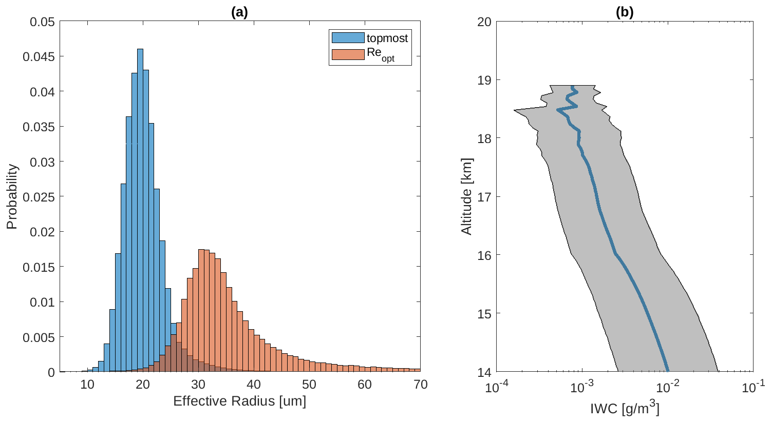
Figure 2 Cloud statistics based on 98 293 overshooting deep convective samples from the DARDAR-Cloud dataset. The samples are within 1000 km of a tropical cyclone center. (a) Histograms of the effective radius (µm) of cloud ice particles at the topmost layer (blue) and the effective radius for representing vertically uniform optical properties (R_e,opt, red). (b) Mean IWC (blue curve) and SD of the IWC (gray area).

Using the identified OT-DCC profiles from DARDAR-Cloud, we calculate the probability distribution function (PDF) of the effective radii of ice particles at the topmost cloud layer. Figure 2a shows that the ice particles are typically small, with an average effective radius of 21.5 µm and 1st and 99th percentiles of 13.3 and 39.7 µm, respectively. Using the same OT-DCC profiles, profiles of the mean and standard deviation (SD) of the IWC are obtained and are shown in Fig. 2b. The statistical calculations performed here exclude zero values. The average cloud-top height is 16.7 km.

Baum et al. (2011) developed a model of habit mixture as a function of ice particle size for tropical deep convective clouds. Using this model, ice cloud optical properties are generated following the description in Sect. 2.2. A radiance spectrum calculated using this model is indicated by the subscript “mix.” Based on the habit mixture model, over 80 % of small ice particles in tropical deep convection are solid columns. Therefore, we also generate the radiance from ice cloud optical properties using solid columns alone, and this is indicated by the subscript “sc.”

100 profiles are selected from the OT-DCC samples. For each sample, we calculate the upwelling infrared radiance R_mix(R_e,IWC) using the IWC profile, effective radius (R_e) profile, and the habit mixture model developed by Baum et al. (2011). The mean temperature (t₀) and water vapor (q₀) profiles of the NWP simulation domain (Fig. 1) are used in the radiative transfer calculations.

Considering that the infrared radiance spectra may not be sensitive to vertical variations in cloud optical properties, we assume that optical properties are constant in all vertical layers of an atmospheric column and a crystal habit of solid columns to simplify the input cloud variables for MODTRAN. Following this assumption, we calculate $R_{\mathrm{sc}}(R_{\mathrm{e},\mathrm{opt}},\mathrm{IWC})$ using solid columns alone and one effective radius value, R_e,opt, for all vertical layers of an individual profile. This R_e,opt, which minimizes the brightness temperature difference between R_mix(R_e,IWC) and $R_{\mathrm{sc}}(R_{\mathrm{e},\mathrm{opt}},\mathrm{IWC})$, is solved iteratively. The PDF of R_e,opt is shown in red in Fig. 2a; it has an average of 34 µm (R_e,0) and a SD of 11 µm. In practice, one may estimate R_e,opt from the effective radius of a cloud layer where the optical depth measured from the cloud top reaches unity, in which case the root-mean-square error (RMSE) is 1.6 µm (∼ 5 %). The spectrum of the RMSE in $R_{\mathrm{sc}}(R_{\mathrm{e},\mathrm{opt}},\mathrm{IWC})$ relative to R_mix(R_e,IWC) is shown by the red solid curve in Fig. 3a. The magnitude of this RMSE spectrum in the mid-infrared is around 0.1 K, confirming that the mid-infrared spectrum is not sensitive to layer-to-layer variations in effective radius or to mixtures of crystal habits that differ from solid columns. A reasonable representation of the mid-infrared emission spectrum of a tropical deep convective cloud can be obtained by assuming constant cloud optical properties for the entire column of the cloud. At wavenumbers higher than 1800 cm⁻¹, however, neglecting the variations in effective radius and crystal habit induces significant RMSE, as shown in Fig. 3a. The RMSE spectrum is also computed by adopting an AIRS-like spectral response function, ε_synergistic, to represent the forward model uncertainty in the synergistic retrieval method introduced in Sect. 2.3.

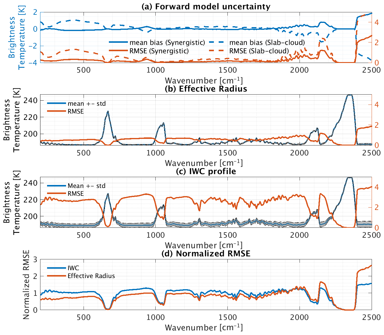
Figure 3 Effects of variations in tropical deep convective clouds on infrared radiance spectra from 200 to 2500 cm⁻¹ at 5 cm⁻¹ resolution. (a) The mean bias (blue, left y axis) and RMSE (red, right y axis) in $R_{\mathrm{sc}}(R_{\mathrm{e},\mathrm{opt}},\mathrm{IWC})$ (solid) and $R_{\mathrm{sc}}(R_{\mathrm{e},\mathrm{opt}},\mathrm{slab})$ (dashed), respectively, relative to R_mix(R_e,IWC). (b) The mean radiance spectrum of $R_{\mathrm{sc}}(R_{\mathrm{e},\mathrm{opt}},{\mathrm{IWC}}_{\mathrm{0}})$ (blue, left y axis) and its SD (gray area). Red curves (right y axis) show the RMSE in $R_{\mathrm{sc}}(R_{\mathrm{e},\mathrm{0}},\mathrm{IWC})$ relative to $R_{\mathrm{sc}}(R_{\mathrm{e},\mathrm{opt}},\mathrm{IWC})$. (c) The mean radiance spectrum of $R_{\mathrm{sc}}(R_{\mathrm{e},\mathrm{0}},\mathrm{IWC})$ (blue, left y axis) and its SD (gray area). Red curves (right y axis) show the RMSE in $R_{\mathrm{sc}}(R_{\mathrm{e},\mathrm{opt}},{\mathrm{IWC}}_{\mathrm{0}})$ relative to $R_{\mathrm{sc}}(R_{\mathrm{e},\mathrm{opt}},\mathrm{IWC})$. (d) The RMSE in $R_{\mathrm{sc}}(R_{\mathrm{e},\mathrm{0}},\mathrm{IWC})$ relative to $R_{\mathrm{sc}}(R_{\mathrm{e},\mathrm{opt}},\mathrm{IWC})$ (blue) and the RMSE in $R_{\mathrm{sc}}(R_{\mathrm{e},\mathrm{opt}},{\mathrm{IWC}}_{\mathrm{0}})$ relative to $R_{\mathrm{sc}}(R_{\mathrm{e},\mathrm{opt}},\mathrm{IWC})$ (red); both are also normalized to the spectral mean.

In the following, the R_e,opt determined for each profile as described above is used to represent the vertically constant effective radius value for characterizing the cloud optical properties of a cloud column. It is also used to evaluate the spectral differences caused by IWC and column-to-column variations in cloud optical properties. We calculate infrared radiance spectra with the mean effective radius (R_e,0, 34 µm) or IWC profile (IWC₀), denoted $R_{\mathrm{sc}}(R_{\mathrm{e},\mathrm{0}},\mathrm{IWC})$ and $R_{\mathrm{sc}}(R_{\mathrm{e},\mathrm{opt}},{\mathrm{IWC}}_{\mathrm{0}})$, respectively. Perturbations of infrared spectra caused by variations in effective radius (R_e,opt) are then evaluated using the mean (blue curve) and the SD (gray-shaded area) of the equivalent brightness temperature of $R_{\mathrm{sc}}(R_{\mathrm{e},\mathrm{opt}},{\mathrm{IWC}}_{\mathrm{0}})$, as shown in Fig. 3b. Using the mean effective radius leads to a RMSE spectrum in $R_{\mathrm{sc}}(R_{\mathrm{e},\mathrm{0}},\mathrm{IWC})$ relative to $R_{\mathrm{sc}}(R_{\mathrm{e},\mathrm{opt}},\mathrm{IWC})$, as shown by the red curve in Fig. 3b. Similar results are shown in Fig. 3c for the IWC.

In Fig. 3b and c, the mean spectrum of OT-DCCs shows cold and relatively uniform brightness temperatures in the window and weak absorption channels that largely correspond to the emission from the cloud top. While variations in the effective radius (R_e,opt) and IWC have only a weak effect on the strong absorption channels, they greatly impact the cloud emission, thus leading to large radiance variations in the window and weak absorption channels. As a result, the two RMSE spectra are similar. The RMSE due to column-to-column variations in effective radius (R_e,opt) is around 1 K, and the RMSE due to a varying IWC profile is around 3 K.

The RMSE spectra are further normalized with respect to the spectral mean, as shown in Fig. 3d, to examine whether the spectral signatures of the effective radius and IWC are distinguishable from each other. Despite the overall similarity, the effective radius affects the spectrally dependent extinction coefficients, leading to a tilted pattern across the infrared spectra, while the RMSE due to the IWC is relatively uniform across the infrared window. Therefore, it is possible to distinguish the radiative signals of the effective radius from those of the IWC with a mid-infrared coverage characteristic of existing instruments. Interestingly, differences in the two normalized RMSE spectra are more prominent at lower wavenumbers (∼ 200 cm⁻¹), suggesting that far-infrared channels – e.g., those from future instruments such as FORUM (Palchetti et al., 2020) and TICFIRE (Blanchet et al., 2011) – may be advantageous for UTLS retrieval. This is beyond the scope of the present simulation experiment but warrants future investigation.

To enable a comparison, we follow Feng and Huang (2018) in obtaining the infrared spectra using the slab-cloud method. For each R_mix(R_e,IWC), we calculate the brightness temperature of the window channel at 1231 cm⁻¹. The idea of the slab-cloud method used by Feng and Huang (2018) is to minimize the infrared radiance residual at this window channel by placing a slab of cloud at the vertical layer where the atmospheric temperature differs the least from BT₁₂₃₁. This 500 m thick slab of cloud has a uniform IWC of 1.5 g m⁻³ and an effective radius of 34 µm. The temperature of this vertical layer is adjusted to BT₁₂₃₁. With this prescribed cloud layer in place, radiance spectra denoted $R_{\mathrm{sc}}(R_{\mathrm{e},\mathrm{0}},\mathrm{slab})$ are calculated again for each profile. The BT₁₂₃₁ values of R_mix(R_e,IWC) and $R_{\mathrm{sc}}(R_{\mathrm{e},\mathrm{0}},\mathrm{slab})$ are identical. Consequently, the differences between R_mix(R_e,IWC) and $R_{\mathrm{sc}}(R_{\mathrm{e},\mathrm{0}},\mathrm{slab})$ in other channels highlight the radiance uncertainty due to the slab-cloud assumption. The RMSE in $R_{\mathrm{sc}}(R_{\mathrm{e},\mathrm{0}},\mathrm{slab})$ relative to R_mix(R_e,IWC) is shown by the dashed red curve in Fig. 3a.

Figure 3a reveals that the slab-cloud assumption cannot fully account for the spectral variations in cloud emission. This assumption leads to a spectrally tilted mean radiance bias, as shown by the red curve in Fig. 3a. We note that this tilted pattern is related to the spectrally dependent extinction coefficient, which is affected by the effective radius (the variation in R_e,opt) so that radiances at different wavenumbers are contributed by cloud emission at different heights, which is in turn affected by the vertical distribution of ice mass. Therefore, the clear-cut cloud boundary in the slab cloud and the constant effective radius (R_e,opt) collectively contribute to the radiance bias shown by the dashed blue curve in Fig. 3a. The RMSE of $R_{\mathrm{sc}}(R_{\mathrm{e},\mathrm{0}},\mathrm{slab})$ shows a minimum of around 0.2 K in the mid-infrared window and a maximum of over 4 K at high wavenumbers (over 2000 cm⁻¹). This RMSE spectrum is also calculated by adopting an AIRS-like spectral response function to represent the radiance uncertainty induced by the slab-cloud assumption in the retrieval described in Sect. 2.3, and is denoted ε_slab.

2.3 Retrieval algorithm

The cloud-assisted retrieval proposed by Feng and Huang (2018) is an optimal estimation method (Rodgers, 2000) that retrieves atmospheric states above clouds using infrared spectral radiance. Similar to Eq. (1) in Feng and Huang (2018), we express the relation between the observation vector y and the state vector x as follows:

$$\begin{array}{}\text{(1)}& {\displaystyle }\mathit{y}& {\displaystyle }=F\left({\mathit{x}}_{\mathrm{0}}\right)+{\displaystyle \frac{\partial F}{\partial \mathit{x}}}\left(\mathit{x}-{\mathit{x}}_{\mathrm{0}}\right)+\mathit{\epsilon }\text{(2)}& {\displaystyle }& {\displaystyle }={\mathit{y}}_{\mathrm{0}}+\mathbf{K}\left(\mathit{x}-{\mathit{x}}_{\mathrm{0}}\right)+\mathit{\epsilon }.\end{array}$$

Using a similar definition to that in Feng and Huang (2018), the state vector includes the temperature x_t and the logarithm of specific humidity x_q in 67 model layers. x₀ refers to the first guess for the state vector, which is the mean of the a priori dataset. y contains the infrared radiance observations y_rad. F is the forward model that relates x to y. Here, the forward model is the radiative transfer model, MODTRAN 6.0, configured with the spectral response function of the AIRS instrument. The forward model can be linearly approximated by the Jacobian matrix K, which is iteratively computed at every time step. ε is the measurement error, which includes the radiometric uncertainties of the instrument and the forward model error. The forward model error comes from the radiative transfer algorithm used by the forward model and from inputs to the forward model. Because the line-by-line algorithm of MODTRAN has been validated against LBLRTM (Berk and Hawes, 2017), we consider the forward model error to mainly arise from the uncertainties in the inputs, namely the cloud assumptions in the radiative transfer simulation, which is evaluated in Sect. 2.2.1. Other uncertainties in the forward model calculations are neglected.

Following the optimal estimation method (Rodgers, 2000, Eq. 5.16), an estimate of x, denoted $\widehat{\mathit{x}}$, is expressed as

$$\begin{array}{}\text{(3)}& {\displaystyle }\widehat{\mathit{x}}={\mathit{x}}_{\mathrm{0}}+\mathbf{GK}\left(\mathit{x}-{\mathit{x}}_{\mathrm{0}}\right)+\mathbf{G}\left(\mathit{y}-\mathbf{K}\mathit{x}\right)\text{(4)}& {\displaystyle }\mathbf{G}={\mathbf{S}}_{\mathrm{a}}{\mathbf{K}}^T{\left({\mathbf{KS}}_{\mathrm{a}}{\mathbf{K}}^T+{\mathbf{S}}_{\mathit{\epsilon }}\right)}^{-\mathrm{1}},\end{array}$$

where S_a and S_ε are the covariance matrix of the state vector as given by the a priori dataset and that of the error in the observation vector, respectively. S_ε is set to be a diagonal matrix because the observation errors in different channels are considered to be uncorrelated.

$\widehat{\mathit{x}}$ can then be solved iteratively via

$$\begin{array}{}\text{(5)}& \begin{array}{rl}{\widehat{\mathit{x}}}_{i+\mathrm{1}}& ={\mathit{x}}_{\mathrm{0}}+{\left({\mathbf{K}}_i^T{\mathbf{S}}_{\mathit{\epsilon }}^{-\mathrm{1}}{\mathbf{K}}_i+{\mathbf{S}}_{\mathrm{a}}^{-\mathrm{1}}\right)}^{-\mathrm{1}}{\mathbf{K}}_i^T{\mathbf{S}}_{\mathit{\epsilon }}^{-\mathrm{1}}\left[\mathit{y}-F\left(\widehat{{\mathit{x}}_i}\right)\right.\\ & \left.+{\mathbf{K}}_i\left({\widehat{\mathit{x}}}_i-{\mathit{x}}_{\mathrm{0}}\right)\right],\end{array}\end{array}$$

where the subscript i refers to the ith iteration step.

The equations described above are adopted from Feng and Huang (2018), where the state vector x includes the temperature and the logarithm of specific humidity. For comparison, we adopt the slab-cloud retrieval scheme of Feng and Huang (2018) as described above and refer to the result as the slab-cloud retrieval in the following. The only difference from Feng and Huang (2018) is in S_ε. While S_ε is the square of the radiometric noise of the AIRS instrument in Feng and Huang (2018), in this study using the slab-cloud retrieval scheme, S_ε contains the sum of the square of radiometric noise and the square of ε_slab (as schematically depicted by the dashed red curve in Fig. 3a) to account for radiance uncertainties induced by the slab-cloud assumption. Because ε_slab is relatively small, especially at absorption channels, we find that adding off-diagonal correlations to S_ε does not improve the retrieval quality significantly. Therefore, S_ε keeps its diagonal form.

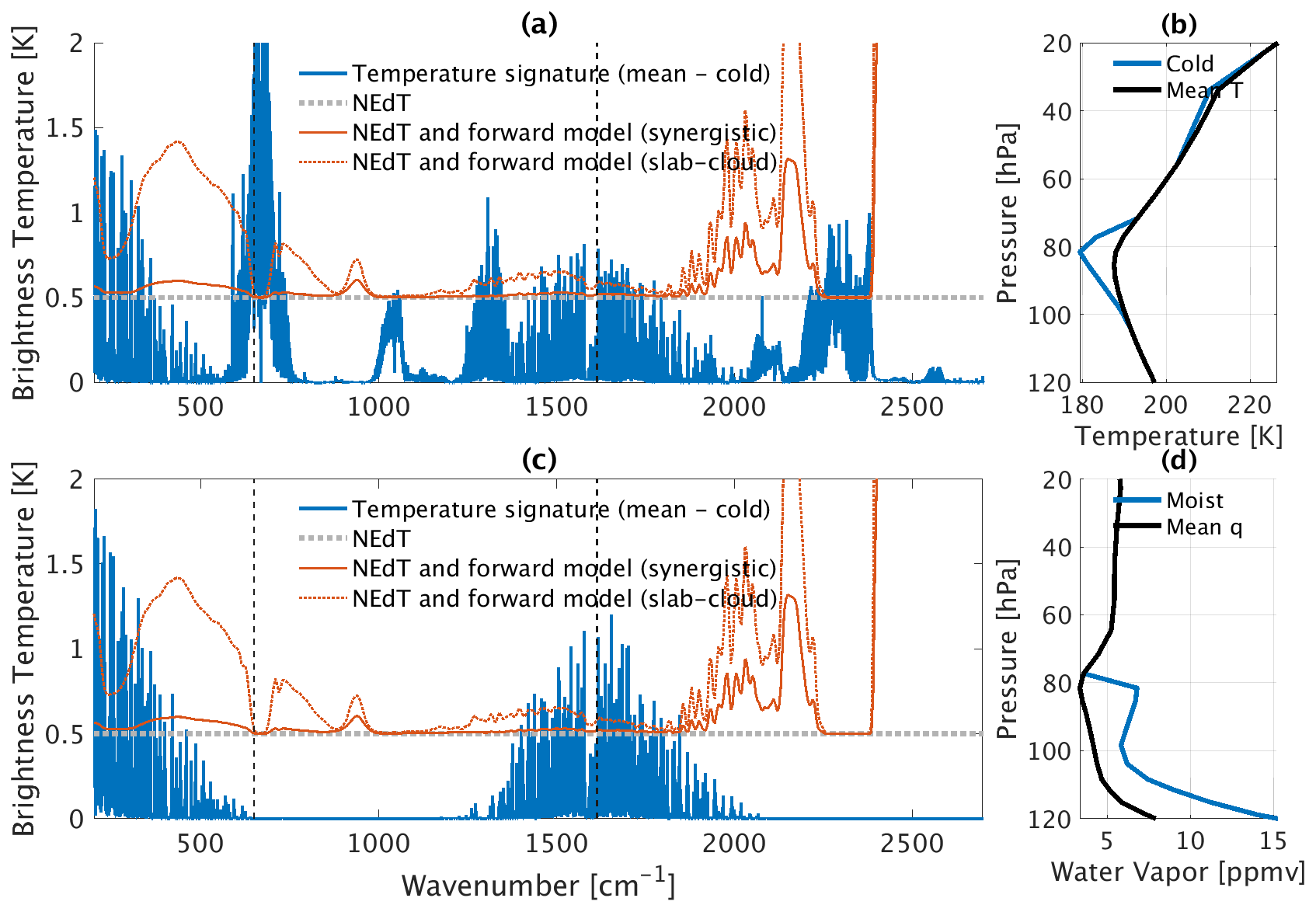
Figure 4 Spectral signals of above-storm atmospheric variations in (a) temperature and (c) water vapor from 200 to 2500 cm⁻¹. The signals are obtained by differencing the upwelling radiance spectra at the TOA simulated from the mean of all profiles (black curves in panels b and d) and radiance spectra simulated from the mean of the profiles with overshooting convective clouds near the cyclone center (blue curves in panels b and d). These signals are shown at a spectral resolution of 0.1 cm⁻¹. In (a) and (c), the dotted light gray lines denote a NEdT of 0.5 K (characterizing the AIRS instrument at cold scene temperature). The solid red lines denote the uncertainties for a combination of the NEdT and ε_synergistic and the dotted red lines denote those for a combination of the NEdT and ε_slab, which are convoluted at 5 cm⁻¹ spectral intervals in this plot. The AIRS spectral range used in this study is 649.6–1613.9 cm⁻¹ and is marked by dashed dark gray lines.

We further examine whether the addition of ε_slab masks spectral signals from atmospheric variations. Figure 1 shows that strong cooling and hydration appear above overshooting DCCs near the cyclone center (141^∘ E, 16^∘ N). We denote the mean profiles of temperature and water vapor in this region as t_cold and q_mois, respectively, and these are shown in Fig. 4b, d (blue curves). A set of radiative transfer calculations are conducted to obtain $R_{\mathrm{sc}}(R_{\mathrm{e},\mathrm{0}},t_{\mathrm{0}},q_{\mathrm{0}})$, $R_{\mathrm{sc}}(R_{\mathrm{e},\mathrm{0}},t_{\mathrm{cold}},q_{\mathrm{mois}})$, and $R_{\mathrm{sc}}(R_{\mathrm{e},\mathrm{0}},t_{\mathrm{cold}},q_{\mathrm{0}})$ at 0.1 cm⁻¹ spectral resolution using an effective radius of 34 µm and a randomly selected IWC profile (cloud top at 100 hPa) for this region. The spectral signals for temperature and water vapor are then obtained from $R_{\mathrm{sc}}(R_{\mathrm{e},\mathrm{0}},t_{\mathrm{0}},q_{\mathrm{0}})-R_{\mathrm{sc}}(R_{\mathrm{e},\mathrm{0}},t_{\mathrm{cold}},q_{\mathrm{0}})$ and $R_{\mathrm{sc}}(R_{\mathrm{e},\mathrm{0}},t_{\mathrm{0}},q_{\mathrm{0}})-R_{\mathrm{sc}}(R_{\mathrm{e},\mathrm{0}},t_{\mathrm{0}},q_{\mathrm{mois}})$, respectively. The signal strength under different spectral specifications was examined by Feng and Huang (2018) and that investigation is not repeated here. The spectral signals are compared to the radiance uncertainties in Fig. 4. The spectral range used in the retrieval tests (between 649.6 and 1613.9 cm⁻¹) is demarcated by dotted gray lines in Fig. 4.

Figure 4 shows that the radiance uncertainty from using the slab-cloud assumption, ε_slab, does not completely obscure the temperature signal or water vapor signal. In the CO₂ and water vapor channels, where the signal is the strongest, the TOA radiance spectra are not as sensitive to cloud emission due to strong atmospheric attenuation in these channels. ε_slab becomes greater in the wings of absorption channels, where the signals are already masked by the instrumental NEdT of ∼ 0.5 K.

2.3.1 Synergistic method

The radiance uncertainty due to the slab-cloud assumption, ε_slab, can be largely eliminated by incorporating collocated observations of cloud profiles from active sensors (CloudSat-CALIPSO) along the same track as the hyperspectral infrared sounder (such as AIRS). Motivated by the work of Turner and Blumberg (2018), instead of simply prescribing the cloud profile from the active sensors in the forward model, we include relevant cloud variables in a synergistic retrieval. Turner and Blumberg (2018) demonstrated that additional observation vectors, such as atmospheric and cloud profiles from other instruments or NWP products, can improve convergence in cloudy scenes and retrieval precision by constraining the posterior uncertainty. Following this idea, the observation vector y in Eq. (1) is formulated as: [y_rad,y_other], where y_rad contains the infrared radiance observations and y_other includes elements other than radiance observations; we refer to the latter as the additional observation vector. Collocated cloud observations are added to y_other to mimic cloud properties obtained from the DARDAR-Cloud product. At every iteration step (Eq. 5), the IWC and effective radius are included in the state vector x and are updated along with the temperature and humidity profiles.

In this simulation experiment, the observation vector for the IWC, y_iwc, is set to be the natural logarithm of the IWC profile to account for IWC variations ranging from O(10⁻⁵) to O(1) g m⁻³ and to avoid negative values. Uncertainties in IWC measurements are estimated by averaging the posterior uncertainty of the IWC (provided by the DARDAR-Cloud product for every footprint) in the OT-DCC profiles identified in Sect. 2.2.1. This estimated precision is denoted ε_iwc, and corresponds to an uncertainty in the IWC at vertical levels near the tropopause of roughly 20 %. Then we account for the IWC observation uncertainty by randomly perturbing y_iwc so that y_iwc deviates from the true state by an error that has an SD of ε_iwc. As mentioned in Sect. 2.2, the effective radius profiles of the test set are sampled from the DARDAR-Cloud product. However, we do not intend to retrieve the effective radius profile because mid-infrared radiance spectra are not sensitive to layer-to-layer variations in effective radius, as found in Sect. 2.2.1. Instead, the effective radius for representing the spectral emission of an entire cloud column is retrieved, which is the same as R_e,opt defined in Sect. 2.2.1. The true R_e,opt is obtained by approaching the true radiance spectra through iteration. The observation vector for R_e,opt, ${\mathit{y}}_{R_{\mathrm{e},\mathrm{opt}}}$, is constructed by randomly perturbing the effective radius value at the layer where the optical depth measured from the cloud top reaches unity ($R_{\mathrm{e},\mathit{\tau }=\mathrm{1}}$) with an uncertainty of 5 µm. Note that this prescribed uncertainty is larger than the typical value in the DARDAR-Cloud product (1.6 µm) to account for sampling differences between the instruments. Because the satellite-measured infrared radiance spectra are most sensitive to cloud emission near the cloud top, only the top 1.5 km of the IWC profile in y_iwc is kept, which corresponds to six model layers in the radiative transfer calculations.

The state vector x_iwc contains six layers of the logarithm of the IWC at the same model layers as y_iwc. Note that x_iwc and y_iwc are not required to have the same vertical resolution; in practice, the vertical resolution of y_iwc can be much finer than that of the model layers. The first guess and covariance matrix of x_iwc are calculated using the same a priori dataset described in the previous section, although cross-correlations between the IWC and other atmospheric variables are neglected. Consequently, the forward model for relating x_iwc to y_iwc is a matrix that linearly interpolates the pressure level of x_iwc to match the level of y_iwc (Eq. 6 in Bowman et al., 2006). The a priori value of ${\mathit{x}}_{R_{\mathrm{e},\mathrm{opt}}}$ is 34 µm with an uncertainty range of 11 µm. The diagonal elements of S_ε for y_iwc and ${\mathit{y}}_{R_{\mathrm{e},\mathrm{opt}}}$ are set by conservatively quadrupling the squares of the uncertainty ranges of the variables (20 % for the IWC and 5 µm for R_e,opt).

In this synergistic retrieval framework, cloud optical property inputs to the forward model are considered to be the major source of uncertainties in the forward model. While the IWC and R_e,opt are retrieved states, uncertainties in other cloud variables should be included in the forward model error quantified by ε_synergistic in Sect. 2.2.1. Therefore, the S_ε for y_rad in the synergistic method contains the sum of the square of the radiometric noise and the square of ε_synergistic. As shown in Figs. 3 and 4, ε_synergistic is much smaller than ε_slab and the spectral signals from the temperature and water vapor. It is also smaller than the spectral RMSE caused by the IWC and R_e,opt, with a distinct shape in mean biases (see Fig. 3).

2.3.2 Additional atmospheric observations

Besides the cloud observations, other products that provide collocated atmospheric profiles can be useful for improving the precision of the posterior estimation. These additional products may include atmospheric observations from other instruments that are in the same satellite constellation as the hyperspectral infrared sounder, as well as reanalysis products, which typically do not assimilate cloudy infrared radiances in operation. In this study, we investigate the effect of incorporating coincident reanalysis products by adding an observation vector, y_atm, which contains the temperature and the logarithm of specific humidity at a later time step in the GEM simulation: 810 min after the initial time. This arbitrary choice of simulation time step is intended to represent the potential quantitative differences in temperature, humidity, and cloud fields between a reanalysis product and the true state.

Distributions of retrieval variable fields are shown in Fig. 6. As inferred from the brightness temperature, the massive spatial coverage of DCCs is evident at the time step used as the truth (410 min after the initial time in the GEM simulation). At the later time step (810 min), the atmospheric data used as y_atm are taken from the same locations but deviate from the truth as they are not directly above convective overshoots at this time step. The RMSE between atmospheric profiles from the two time steps (410 and 810 min) defines the uncertainties in y_atm. To be conservative, the uncertainty in y_atm is set to quadruple the square of the RMSE in the corresponding diagonal elements of S_ε.

3 Results

Four retrieval cases are examined to assess the retrieval performance achieved using different strategies. Among them, Cases 1 and 2 use the slab-cloud method whereas Cases 3 and 4 use the synergistic method that incorporates cloud observations. Cases 2 and 4 differ from Cases 1 and 3 in that they include y_atm in the retrieval. The components of the state and observation vectors for the four cases are listed in Table 1. An additional case is also performed, Case 5, which follows the same optimal estimation framework as in Case 4 without using the infrared radiances y_rad. It is expected to converge to a posterior state that is jointly determined by the a priori profile, y_iwc, and y_atm. Therefore, the statistical differences between Case 4 and 5 indicate the improvements attributable to infrared radiances (as opposed to other sources of information). Case 5 is relatively uniform in space and is therefore not included in the figures, but it is listed in Tables 1 and 2 for comparison. Following the framework of this simulation experiment, retrievals are then performed for the 100-profile test set, using the synthetic radiance observations (y_rad) generated in Sect. 2.2, the IWC (y_iwc) and effective radius (${\mathit{y}}_{R_{\mathrm{e},\mathrm{opt}}}$) described in Sect. 2.3.1, and the additional atmospheric product (y_atm) constructed in Sect. 2.3.2. Retrieval performance is assessed by examining the mean biases and RMSEs in Figs. 5 and 6. Retrieved temperature, water vapor, and IWC profiles are also compared to the first guess, observation constraints (y_other), and the truth in Fig. 7 for two samples from the test set.

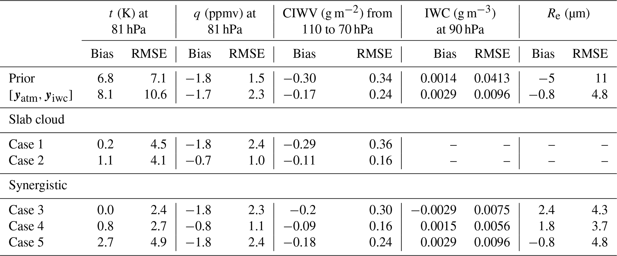
Table 1 State vector and observation vector in four retrieval strategy cases. Case 5 is a posterior estimation of the state vector from a combination of y_atm, y_iwc, ${\mathit{y}}_{R_{\mathrm{e},\mathrm{opt}}}$, and the a priori profile. DFS is compared to the number of vertical layers of the state vector. DFS is counted from 130 to 13.5 hPa for temperature and water vapor (20 model layers).

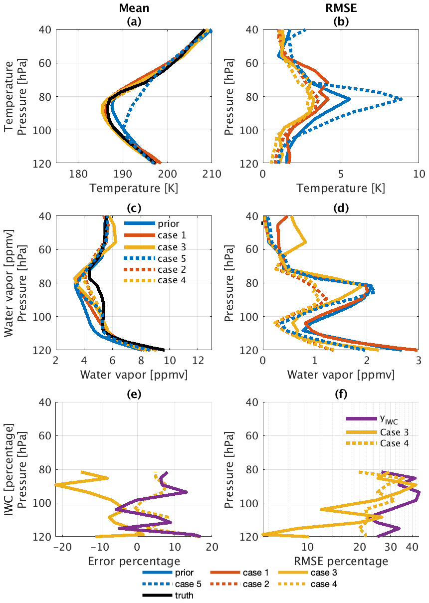
Figure 5 Profiles of the mean and RMSE of the temperature (a, b) and water vapor (c, d) for the four retrieval strategy cases. Profiles of the percent mean bias (e) and RMSE (f) of the IWC are also shown. Blue curves show the bias and RMSE in the prior. Red curves refer to cases where the retrieval strategy uses the slab-cloud method (solid lines for Case 1 and dotted lines for Case 2), while yellow curves refer to cases where the retrieval strategy uses the synergistic method (solid lines for Case 3 and dotted lines for Case 4).

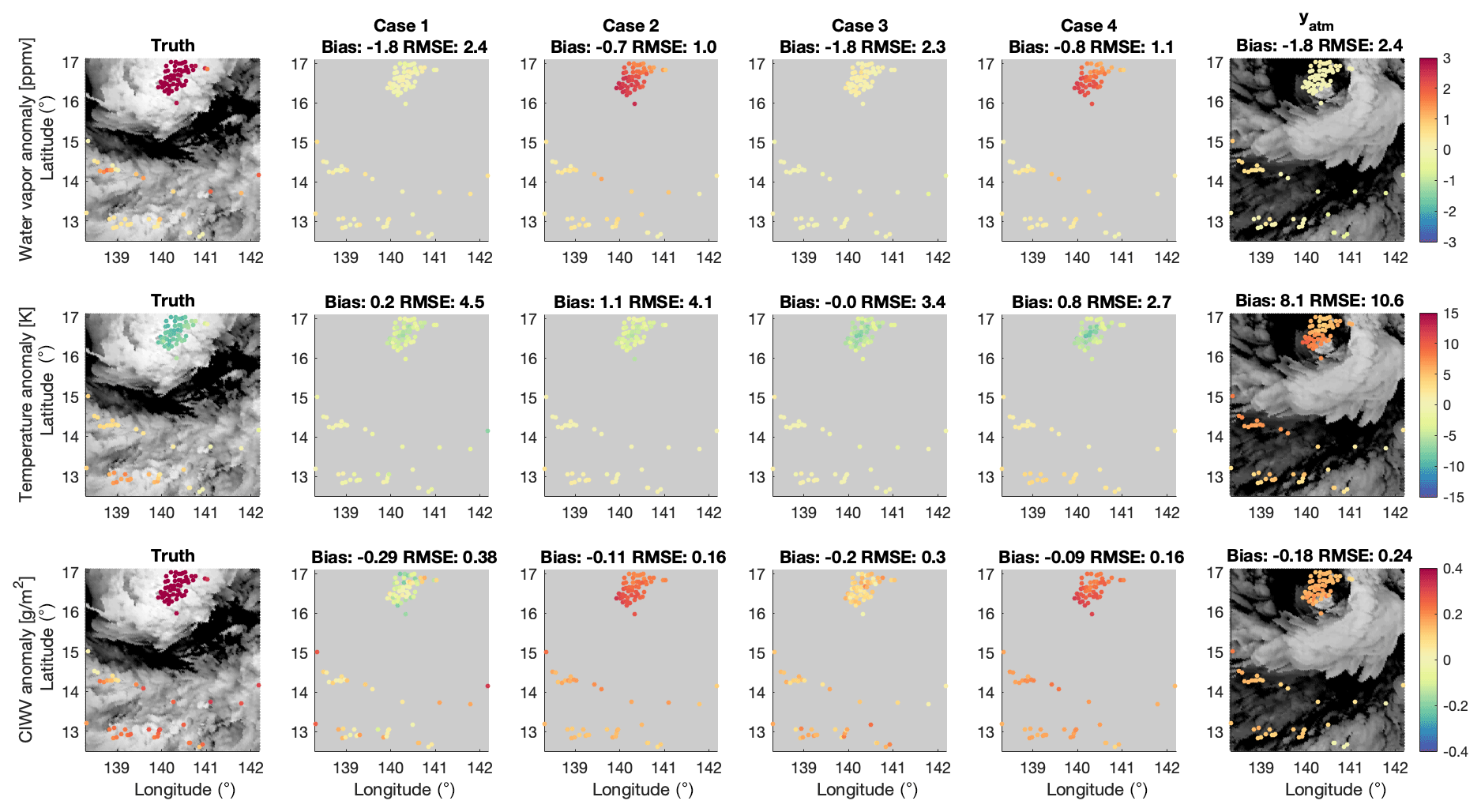
Figure 6 Horizontal distributions of the anomalies (defined as the deviation from x₀) in water vapor (in ppmv, upper panels), temperature (in K, middle panels) at 81 hPa, and column integrated water vapor between 110 and 70 hPa (in g m⁻², lower panels). The true states are shown in the first column, with the BT₁₂₃₁ distribution shown in the background of each panel via gray shading. The second to fifth columns show retrieved results for the four retrieval strategy cases described in Table 1. The sixth column shows the distribution of the additional observation vector, y_atm, incorporated into the retrievals in Cases 2 and 4. This additional atmospheric constraint (y_atm) is taken from the model fields 810 min after the initial simulation time step.

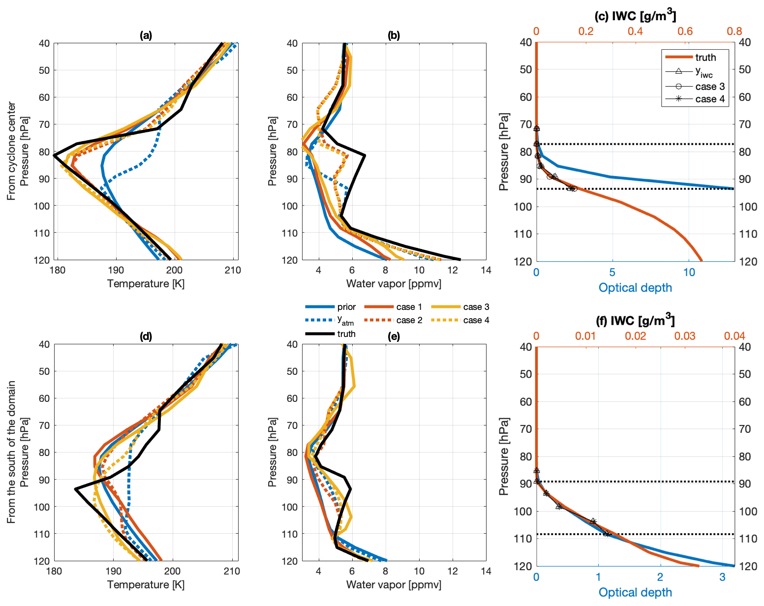
Figure 7 Temperature (a, d) and water vapor (b, e) profiles of the first guess (solid blue lines), truth (solid black lines), and posterior results (red and yellow lines represent the slab-cloud and synergistic methods, respectively; the solid lines refer to cases without y_atm and the dotted lines to cases that include y_atm) for two profiles from the test set. (c, f) True IWC (red curve and upper x axis) and all-sky optical depth from the TOA (blue curve and lower x axis) for the two selected profiles. The y_iwc and retrieved IWC profile are indicated by triangles, circles (Case 3), and asterisks (Case 4), respectively. Dotted black lines mark the vertical ranges of ice cloud information included in y_iwc and x_iwc, while ice clouds at the lower vertical levels are prescribed to be the same as the observed cloud.

We next examine the DFS (degrees of freedom for signal; Rodgers, 2000) of the temperature, water vapor, IWC, and effective radius in the four retrieval cases (Table 1​​​​​​​). DFS is defined as the trace of the averaging kernel A, which relates the retrieved state $\widehat{\mathit{x}}$ to the true state x₀ , as derived from Eq. (5)​​​​​​​ at the end of the iteration:

$$\begin{array}{}\text{(6)}& {\displaystyle }\widehat{\mathit{x}}-{\mathit{x}}_{\mathrm{0}}=\mathbf{A}\left(\mathit{x}-{\mathit{x}}_{\mathrm{0}}\right)\text{(7)}& {\displaystyle }\mathbf{A}={\left({\mathbf{K}}^T{\mathbf{S}}_{\mathit{\epsilon }}^{-\mathrm{1}}\mathbf{K}+{\mathbf{S}}_{\mathrm{a}}^{-\mathrm{1}}\right)}^{-\mathrm{1}}{\mathbf{K}}^T{\mathbf{S}}_{\mathit{\epsilon }}^{-\mathrm{1}}\mathbf{K}.\end{array}$$

While all observation vectors are used in the retrieval, only the radiance observation y_rad is included to calculate the DFS, so a higher DFS indicates higher information content brought by y_rad alone. Because the DFS depends on the cloud distribution, the DFS shown in Table 1 is averaged over the 100-profile test set.

Although ε_slab does not mask the observable signals in Fig. 4a and b, the DFS for temperature increases from 3.15 (Case 1) to 3.6 (Case 3) when the synergistic method is adopted. This improved DFS highlights the strong sensitivity of the synergistic method to the temperature near the cloud top. In comparison, the slab-cloud method fails to fully capitalize on information near the cloud top as it neglects contributions from the vertical layers around the assumed sharp cloud boundary. Therefore, the synergistic method is expected to achieve a better result for temperature.

Moreover, significant DFS values are found for the IWC (1.94 out of 6, on average) and effective radius (0.66 out of 1, on average). The DFS confirms the sensitivity of infrared radiances to the IWC profile and effective radius near the cloud top, which is consistent with the large radiative perturbation caused by varying IWC (Fig. 3c–d) based on the DARDAR-Cloud product. The DFS for IWC varies from 0.96 to 2.71 in the test set, depending on the optical depth near the cloud top. Low ice density near the cloud top leads to a higher DFS for IWC and effective radius. For example, the DFS for IWC increases from 1.30 in Fig. 7c to 2.63 in Fig. 7f because thermal emission from lower levels can be transmitted through the topmost cloud layer. In the meantime, the DFS for effective radius increases from 0.04 to 0.66 because the thermal emission is more sensitive to the spectral shape of extinction coefficients induced by the effective radius (as depicted in Fig. 3c) when the optical depth is small. Overall, the DFS values suggest that the synergistic method can improve the precision of IWC and effective radius measurements relative to collocated cloud products alone.

Retrieval performance is evaluated through the mean bias and RMSE in temperature, humidity, and IWC between each retrieved profile and the truth, as shown in Fig. 5. The retrieval performance is also evaluated with regard to these quantities at selected levels and with regard to CIWV integrated from 110 to 70 hPa.

3.1 Slab-cloud retrieval

Improving upon Feng and Huang (2018), Case 1 accounts for the radiance uncertainties due to the slab-cloud assumption, while Case 2 further incorporates additional atmospheric constraints to improve the precision of the method.

The results for Case 1 are shown as solid red curves in Figs. 5 and 7. The major improvement in Case 1 as compared to the prior (solid blue curves) is in the temperature profile from 100 to 75 hPa. Although the DFS for water vapor reaches 0.69, Case 1 does not provide much of an improvement in water vapor from the first guess.

Table 2 Performance assessment of four retrieval strategy cases. The cases are compared with the prior, the observation vector, and Case 5.

Case 2 improves upon Case 1 owing to the information carried by the additional atmospheric constraints, y_atm. Case 2 is represented by the dotted red curves in Figs. 5 and 7. It approaches the true state better than Case 1, despite warm and dry biases in the first guess and y_atm (see Fig. 5a, c). Notably, it increases the retrieved water vapor concentration by around 1 ppmv on average and reduces the RMSE from 2.4 to 1.0 ppmv, as shown in Fig. 5c, d and Table 2​​​​​​​. Case 2 reduces the RMSE in the CIWV by half when compared to Case 1.

To demonstrate how well the retrieved atmospheric field represents the spatial variability in the true state (Fig. 1), namely the moister and colder UTLS region in the cyclone center compared to the south of the domain, the distributions of water vapor, temperature, and CIWV are presented in Fig. 6. It shows that the true spatial patterns are well reproduced by the Case 2 retrieval.

Furthermore, individual profiles from two clusters of overshooting DCCs, which include the DCCs near the cyclone center and those in the south of the domain, are randomly selected to investigate how well the retrieval reproduces the spatial variability in temperature and water vapor. The all-sky optical depths from TOA and IWC profiles for the two locations are shown in Fig. 7c, d. The retrievable signals mainly come from the atmospheric column above thick cloud layers, i.e., where the optical depth is less than 2 (only 13.5 % of the infrared emission is transmitted through this cloud layer).

Figure 7a–c shows results for a location close to the cyclone center. At this location, the slab-cloud method prescribes the cloud layer to be located at the cold point due to the strong cloud emission. Atmospheric anomalies above 86 hPa have an impact on TOA infrared radiances. Around 80 hPa, the truth profile that we aim to retrieve is around 8 K colder than the prior and nearly 3 ppmv moister. While the result from Case 1 overcomes the bias in temperature, it increases the water vapor over a broad vertical range due – as explained by Feng and Huang (2018) – to the strong smoothing (smearing) effect of the averaging kernel in this case. In comparison, Case 2 correctly produces peak moistening at around 80 hPa while yielding a retrieved temperature profile similar to Case 1.

Figure 7d–f shows the results in a location in the southern part of the domain, where the slab-cloud method prescribes the cloud layer at 95 hPa. At this location, the cloud emission from the top 1.5 km cloud layer affects infrared radiances strongly, as inferred from the optical depth (Fig. 7f), leading to a large radiance residual that cannot be addressed under the slab-cloud assumption. Therefore, Case 1 fails to improve upon the prior. Case 2 leads to a moister posterior compared to the prior owing to the addition of y_atm. However, Case 2 fails to update the temperature profile above the cloud layer. Instead, it approaches y_atm at lower altitudes, leading to an unrealistic vertical oscillation in temperature near 100 hPa.

3.2 Synergistic method

Case 3, which uses the synergistic method, is more sensitive to water vapor and temperature than Case 1, as indicated by the reduced RMSE in Table 2 and the closer match between the retrieved field and the true state in Fig. 6. It retrieves higher water vapor concentrations from 110 to 70 hPa in comparison with Case 1. Owing to the radiative emission from in-cloud layers between 110 and 95 hPa, Cases 3 and 4 become sensitive to the temperature profile near the cloud top. Hence, Cases 3 and 4 reduce the RMSE compared to other cases.

The advantage of the synergistic method, especially when the IWC near the cloud top is relatively small, is illustrated in Fig. 7d–f. At this location, the radiative signal from the moistening near the cloud top can be transmitted to the TOA. As a result, Case 3 approaches the true cloud-top temperature much more closely than Cases 1 and 2 (Fig. 7a, d). It also produces higher water vapor compared to Case 1 (Fig. 7e). Case 4 further benefits from y_atm, which constrains the profile in the vertical range below 110 hPa and above 80 hPa. Case 4 overcomes the warm bias around 90 hPa in y_atm and the first guess. It also reproduces the oscillating temperature feature in Fig. 7d.

Owing to its sensitivity to the IWC and R_e,opt (as suggested by the DFS and Fig. 3), the synergistic method can improve upon the collocated cloud observations by reducing the RMSE in the IWC profile and in R_e,opt (Fig. 5 and Table 2). Although adding y_atm does not significantly improve the retrieval performance in Case 4, it stabilizes the iterative retrieval process by constraining uncertainties in temperature. The improvement attained by using infrared spectra and through the addition of y_atm is desirable to reduce measurement uncertainties caused by sampling differences between the active sensors and the infrared instrument.

While the improvements obtained in Cases 2 and 4 show the advantage of including additional atmospheric products (y_atm), one caveat is the difficulty involved in properly evaluating the uncertainty range, which is included in the covariance matrix of the observation vector. This is important, as the uncertainty range in y_atm constrains the posterior uncertainty range of the retrieval at each vertical level. In this study, we account for the difficulty in evaluating S_ε by increasing the RMSE in y_atm so that the square root of S_ε of y_atm is equivalent to a doubling of the RMSE shown by the blue dotted line in Fig. 5b, d.

Although the additional measurement vector y_atm does not contain the spatial variability pattern seen in Fig. 6, the corresponding covariance in S_ε properly accounts for its variability (uncertainty) by prescribing a large value around 80 hPa but smaller values at other vertical locations. Therefore, it increases confidence in the posterior at levels where the thermodynamic variables are relatively constant. This increased confidence in turn enhances the degrees of freedom in the range around 80 hPa, where the warm and dry signals mainly come from. Therefore, even though y_atm itself deviates from the true state, including y_atm in the optimal estimation can still improve the posterior estimation. In practice, uncertainties in atmospheric products can be estimated by inflating the precision of the product to account for sampling size differences through comparison with NWP models and collocated observations.

4 Conclusion and discussion

Sounding the thermodynamic conditions in the UTLS has long been a challenge. In this work, a simulation experiment was conducted to simulate hypothetical radiance observations of AIRS by integrating a NWP model and a radiative transfer model, MODTRAN 6.0. By conducting the simulation experiment, this study evaluated the ability of existing hyperspectral infrared sounders to detect temperature and humidity fields above convective storms. Our focus was on investigating and constraining the uncertainties induced by clouds. Two retrieval methods were tested: a slab-cloud method that mainly uses infrared radiance measurements (i.e., AIRS) and a synergistic method that combines cloud products from collocated active sensors (i.e., DARDAR-Cloud).

First, we found that a radiative transfer model can simulate the TOA mid-infrared radiance spectra above tropical deep convective clouds fairly accurately (RMSE around 0.1 K, characterized by ε_synergistic) by assuming constant cloud optical properties (per unit mass) in all vertical layers of a cloud column. Uncertainties in the infrared radiance spectra mainly come from variations in the IWC profile and column-to-column variations in effective radius (Fig. 3). The uncertainties are largest in window channels and weak absorption channels because they are sensitive to cloud emission. The slab-cloud assumption locates a clear-cut cloud top that matches the brightness temperature of the window channel. This assumption alleviates, but does not fully eliminate, the cloud effect in the radiance spectrum (Fig. 3a). The remaining radiance uncertainty was accounted for in the retrieval framework of this study and was found to nonsignificantly obscure the temperature and humidity signals in the retrieval. Therefore, we affirmed that the cloud-assisted retrieval proposed by Feng and Huang (2018) improves the sounding of UTLS temperature and water vapor compared to prior knowledge. However, this retrieval neglects information content from the in-cloud atmosphere. As a result, it may lead to biases in individual temperature profiles. For example, as shown in Fig. 7c, the slab-cloud retrieval fails to reproduce oscillating temperature anomalies, although it still detects anomalous moistening above convective storms. Although not explicitly discussed here, a similar OE framework that adopts the slab-cloud assumption would be expected to detect moistening anomalies when applied to other hyperspectral infrared sounders (e.g., IASI and CrIS), due to their similar spectral specifications to AIRS.

Second, especially after incorporating an additional atmospheric constraint, y_atm, we found that the synergistic method is sensitive to temperature, water vapor, the IWC profile, and the column-to-column variation in effective radius. It substantially reduces the RMSE in temperature from 7.1 to 2.7 K compared to the prior. It also reduces the RMSE in column integrated water vapor by half. This method can capture strong moistening features in individual profiles (as shown by Fig. 7b) and detect oscillating temperature anomalies (as shown by Fig. 7c). The temperature and humidity fields retrieved by the synergistic approach best match the true horizontal distribution patterns at a fixed pressure level (Fig. 6). Moreover, owing to the sensitivity of infrared radiance spectra to cloud properties, the synergistic method is able to improve the IWC and effective radius (R_e,opt) relative to collocated active cloud observations.

In conclusion, our study suggests that the synergistic method holds promise as a means to use hyperspectral infrared radiance and cloud profiles from existing instruments (AIRS, CloudSat, and CALIPSO) to retrieve UTLS temperature and water vapor distributions above deep convective clouds. As discussed in Feng and Huang (2018), the sensitivity to water vapor and cloud microphysical properties (see Sect. 2.2.1) could be further improved by including the far-infrared coverage provided by future instruments, e.g., FORUM and TICFIRE. While a limited number of samples are available when applying synergistic retrieval, instruments in geostationary orbit such as IRS (Infrared Spectrometer) and GIIRS (Geostationary Interferometric Infrared Sounder) (Schmit et al., 2009; Holmlund et al., 2021) could greatly increase collocation with other spaceborne active sensors over convective regions. Such an approach may also enhance our understanding of convective impacts by providing time-continuous observations (Li et al., 2018) in future research. The ability of the synergistic method to leverage hyperspectral infrared observations to improve NWP outputs (y_atm) also suggests that the inclusion of cloudy-sky observations in global data assimilation systems, as performed by Okamoto et al. (2020), would be advantageous.