A compact static birefringent interferometer for the measurement of upper atmospheric winds: concept, design and lab performance

A new compact static wind imaging interferometer, called the Birefringent Doppler Wind Imaging Interferometer (BIDWIN), has been developed for the purpose of observing upper atmospheric winds using suitably isolated airglow emissions. The instrument combines a field-widened birefringent delay plate placed between two crossed Wollaston prisms with an imaging system, waveplates and polarizers to produce four fixed 90^∘ phase-stepped images of the interference fringes conjugate to the scene of interest. A four-point algorithm is used to extract line-of-sight Doppler wind measurements across the image of the scene. The arrangement provides a similar throughput to that of a field-widened Michelson interferometer; however, the interferometric component of BIDWIN is smaller, simpler to assemble and less complicated to operate. Consequently, the instrument provides a compact, lightweight and robust alternative that can be constructed and operated with lower cost. In this paper, the instrument concept is presented, and the design and optimization of a prototype version of the instrument are discussed. Characterization of the lab prototype is presented, and the performance of the instrument is examined by applying the instrument to measure a low-velocity two-dimensional Doppler wind field with a high precision (5 m s⁻¹) in the lab.

1 Introduction

Upper atmospheric motions in the mesosphere and lower thermosphere (MLT) region are dominated by large scale tides, planetary waves, as well as large-scale and small-scale gravity waves. Indeed, measurements from space-borne platforms were critical for showing that these waves drive the large-scale circulation in the middle atmosphere (Ern et al., 2016; Geller et al., 2013); however, the processes that govern energy dissipation and interaction remain incompletely understood (Fritts et al., 2016). The MLT region is coupled to the upper atmosphere by wave processes that influence the neutral wind field and subsequently impact ionospheric dynamics. Therefore, understanding this coupling and the mechanisms that influence the dissipation of energy associated with small-scale variability requires the simultaneous spatial sampling of several components of the dynamical fields at resolutions and uncertainties that allow these processes to be resolved.

Passive measurements of Earth's naturally emitted airglow have been used for several decades to remotely measure upper atmospheric motions. Geophysical variability in the region due to the presence of gravity waves and other motions (tides, planetary waves, etc.) perturbs the airglow layer, resulting in variations in the line-of-sight (LOS) Doppler wind and irradiance field (Hines and Tarasick, 1987, 1993). This paper describes the development of a new type of instrument designed to detect these variations. The instrument, called the Birefringent Doppler Wind Imaging Interferometer (BIDWIN), is a compact, high-resolution, large-throughput interferometer constructed with no moving parts.

Several other interferometric techniques have been developed over the past 50 years for the purpose of detecting upper atmospheric motions using airglow emissions. These instruments have provided valuable insights regarding the dynamics occurring in the region. For example, field-widened Michelson interferometers, such as the wide-angle Michelson Doppler imaging interferometer (WAMDII) (Shepherd et al., 1985), the Wind Imaging Interferometer (WINDII) which flew on NASA's Upper Atmosphere Research Satellite (UARS) satellite from 1991 to 2005 (Shepherd, 2002; Shepherd et al., 2012), the mesospheric imaging Michelson interferometer (MIMI) in which a fixed sectored mirror was implemented (Babcock, 2006), as well as the ground-based Michelson Interferometer for Airglow Dynamics Imaging (MIADI) (Langille et al., 2013b) and the E-Region Wind Interferometer (ERWIN) (Gault et al., 1996a; Kristoffersen et al., 2013), have been implemented to measure upper atmospheric motions using airglow emissions. The Fabry–Pérot interferometer and Doppler Asymmetric Spatial Heterodyne (DASH) interferometer have also been implemented to measure upper atmospheric winds (Hays et al., 1993; Killeen et al., 1999; Anderson et al., 2012; Aruliah et al., 2010; Shiokawa et al., 2012; Englert et al., 2007; Harlander et al., 2010).

Making advancements to the field of interferometric wind measurements requires the development of instruments that achieve a similar or better accuracy to what is currently possible but with a higher spatial and temporal resolution using a more robust and less complicated instrument. The core component of the BIDWIN instrument is the field-widened birefringent interferometer (Langille et al., 2013a, 2020) placed between two crossed Wollaston prisms. This configuration produces four images of the scene conjugate to the interference fringes at the detector (see Fig. 3). Appropriate placement of waveplates and polarizers in the system produces four 90^∘ phase-stepped images of the interference fringes. The samples are processed using fringe analysis algorithms like those used in Doppler Michelson interferometry (DMI) to extract LOS winds. A similar birefringent interferometer has been implemented to measure the high-speed motion of plasma in the H1-Heliac at the Australian National University (ANU) (Howard, 2006). However, the capacity of the system to measure low-velocity wind fields (with a precision on the order of <5 m s⁻¹) was not investigated.

The primary advantage of this technique over state-of-the-art field-widened Michelson, Fabry–Pérot and DASH instruments is the mass, volume and minimal complexity in the construction. The interferometer component described in this paper, a birefringent delay plate, has an approximate volume of 10 cm × 5 cm × 5 cm, a mass of ∼1 kg and can be assembled using tools that are available in most optical labs. On the other hand, assembly of the current state-of-the-art instruments requires extreme skill and has only been mastered by a handful of companies, as well as academic and national laboratories. The BIDWIN concept has been developed in collaboration with industry to realize a simple-to-construct instrument capable of performing observations of upper atmospheric winds using low-intensity airglow emissions.

The paper is organized as follows. First, we present the overall requirements, which guide the design of a general high-resolution two-beam interferometer capable of wind measurements with precisions <5 m s⁻¹. These requirements form the basic specifications that drive the design of the BIDWIN instrument. Second, we present the BIDWIN measurement principles and highlight the sensitivity of the technique in comparison to the field-widened Michelson interferometer. Third, the design and optimization of the instrument are presented and the overall sensitivity to wind measurements is examined using simulated ground-based measurements. Fourth, the implementation, characterization and testing of the instrument are presented. Finally, we examine the performance of the design by performing measurements of low-velocity winds produced in the lab.

2 Scientific requirements

2.1 Airglow emissions

The Earth's airglow is naturally emitted in the ultraviolet visible and near-visible spectral regions. The choice of airglow emission lines that can serve as useful tracers for Doppler wind measurements is rather limited. However, measurements have been made both from the ground and from satellites, and several similar instruments are being considered for future ground stations and space missions. Some of these instruments and missions are summarized in Table 1. The list is not exhaustive but is a good summary of the airglow emissions that have been used, or are planned to be used, in wind measurements. All these instruments are wide-field Michelson interferometers except for CLIO (Wang et al., 1993), HRDI (Hays et al., 1993) and TIDI (Killeen et al., 1999), which are Fabry–Pérot interferometers, and MIGHTI, which is a DASH spectrometer (Englert et al., 2007). The emissions consist of O¹S (oxygen green line, 557.7 nm), O¹D (oxygen red line, 630.0 nm), various bands of the Meinel OH system and the ¹Σ and ¹Δ band systems of O₂. The O⁺ lines observed by WINDII yielded little useful data, though there might be potential there for more work.

Table 1 Projects measuring Earth's upper atmospheric winds remotely using Doppler shifts of airglow emissions.

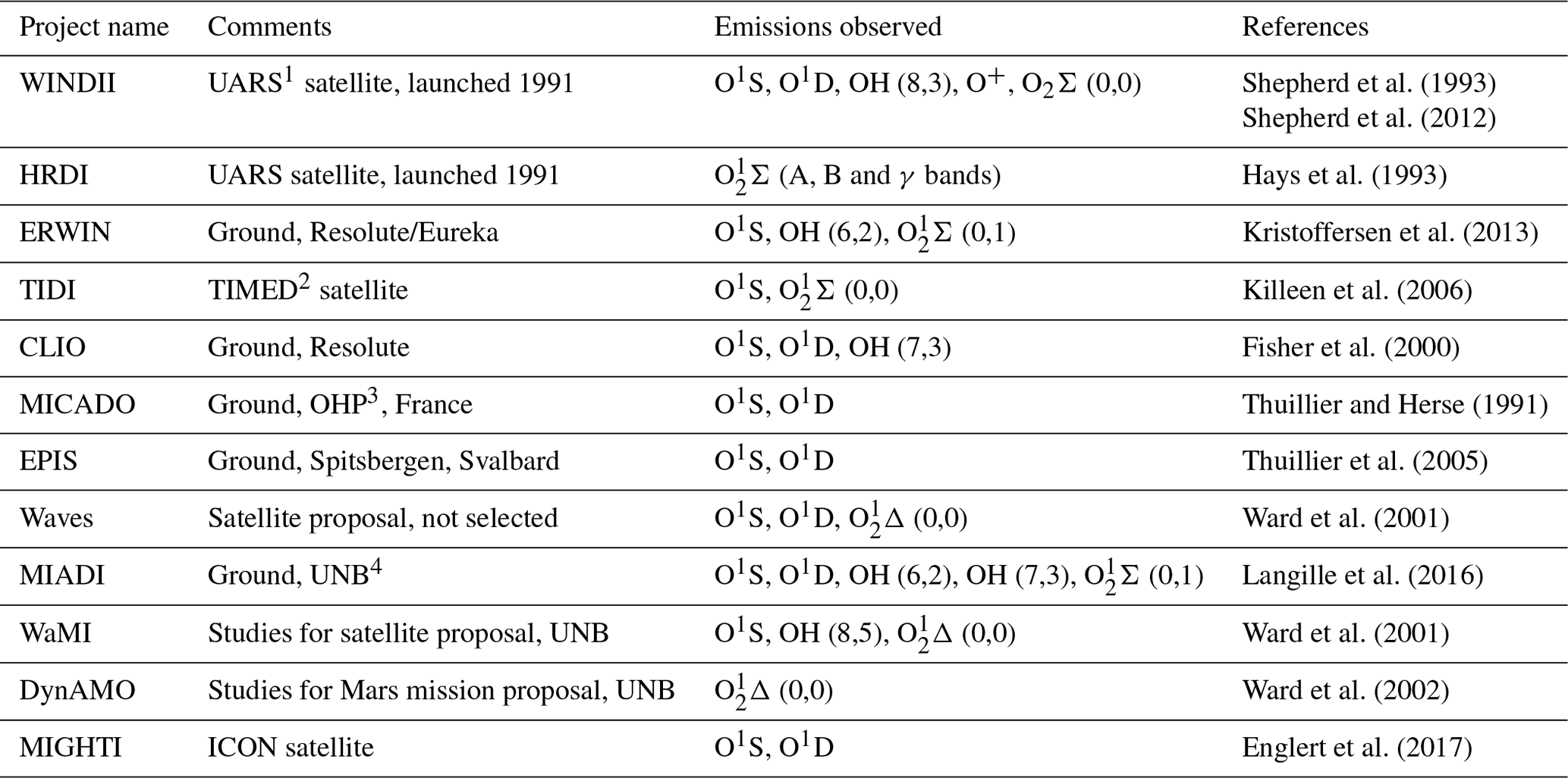
¹ Upper Atmosphere Research Satellite (NASA). ² Thermosphere Ionosphere Mesosphere Energetics and Dynamics satellite. ³ Observatoire de Haute-Provence. ⁴ University of New Brunswick.

Limb-viewing satellite instruments such as MIGHTI (Englert et al., 2017), WINDII (Shepherd et al., 1993), HRDI and TIDI can generate altitude profiles of the wind and can provide high spatial sampling and global coverage. Both nighttime and daytime measurements are possible from a satellite; however, this is not true of measurements made from the ground. Ground-based measurements can only assign a wind to an assumed typical altitude region for the emission being observed and such measurements are only possible at night. If a satellite instrument is properly baffled to protect the optics from scattered sunlight, observations are possible during both day and night. The oxygen emissions (O and O₂) are generally brighter during daytime than nighttime.

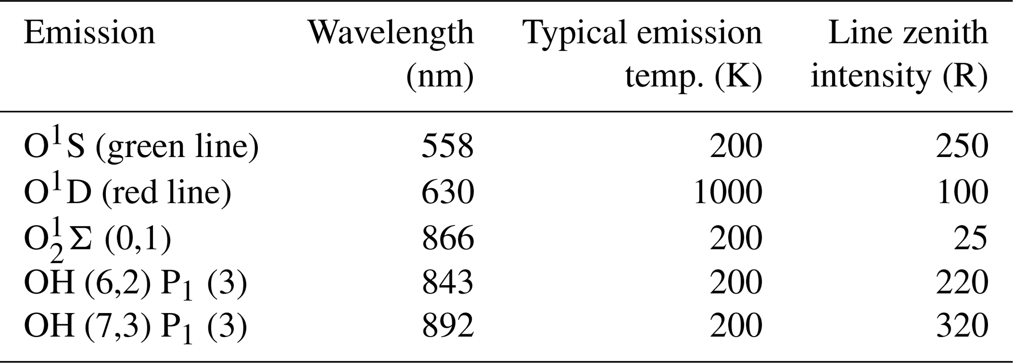
Characteristics of the different lines are given in Table 2 for satellite measurements and in Table 3 for ground-based measurements. The O₂Σ (0,0) and O${}_{\mathrm{2}}^{\mathrm{1}}\mathrm{\Delta }$ (0,0) bands are too strongly self-absorbed to be useful for ground-based measurements. The values in Table 2 for O¹S and O${}_{\mathrm{2}}^{\mathrm{1}}\mathrm{\Delta }$ are from Ward et al. (2001), who refer back to Gault et al. (1996b) for O¹S and to Thomas et al. (1984) and Howell et al. (1990) for O${}_{\mathrm{2}}^{\mathrm{1}}\mathrm{\Delta }$. All the lines listed in Table 2 apart from the molecular oxygen lines provide similar signal levels; however, the sensitivity of the wind measurements made with a two-beam interferometer is also dependent on the line shape, as well as the maximum optical path difference of the interferometer. Therefore, we briefly examine the general principle of wind measurements with a two-beam interferometer and examine the sensitivity of wind measurements made using the lines listed in Table 2.

Table 2 Emissions for Earth satellite (limb) observations.

Table 3 Emissions for ground-based (night) observations.

2.2 Wind measurements using a two-beam interferometer

Measurement of Doppler shifts in spectrally isolated airglow emissions using two-beam interferometers is achieved by sampling the interference pattern produced with an interferometer at several phase steps spanning a full fringe around some large fixed effective path difference. The general measurement process, retrieval algorithms and analytic expressions for the sensitivity of such measurements are described in detail by Kristoffersen et al. (2021). The instrument discussed in this paper samples the interferogram at roughly 90^∘ phase steps. In this case, the intensity of the observed signal can be written as

$$\begin{array}{}\text{(1)}& I_i=I_{\mathrm{0}}\left[\mathrm{1}+UV\cos \left(\mathrm{\Phi }+{\mathit{\phi }}_i\right)\right],\end{array}$$

where I₀ is the mean intensity, U is the instrument visibility, V is the line visibility, and φ_i is the ith phase step. Motion of the source along the line of sight with velocity w results in a slight phase shift in the interferogram given by

$$\begin{array}{}\text{(2)}& \mathit{\delta }\mathrm{\Phi }={\displaystyle \frac{\mathrm{2}\mathit{\pi }D}{c\mathit{\lambda }}}w,\end{array}$$

where λ is the target wavelength, D is the effective path difference, and c is the speed of light. The signal S at the detector is given by

$$\begin{array}{}\text{(3)}& S={\displaystyle \frac{{\mathrm{10}}^{\mathrm{6}}}{\mathrm{4}\mathit{\pi }}}{E}_{\mathrm{0}}A\mathrm{\Omega }\mathit{\tau }\mathit{\eta }t,\end{array}$$

where E₀ is the average emission rate in Rayleighs, A is the collecting area (cm²), Ω is the solid angle (sr) at the location of A, τ is the transmittance, η is the quantum efficiency of the detector, and t is the integration time (s). The product AΩ, called the étendue, is determined by the geometry of the optics. To achieve as large a signal as possible, the instrument should be designed so the product AΩ is as large as possible, within whatever restrictions exist.

Expressions for the uncertainty in the wind measurement were originally developed for the Michelson by Ward (1988) and by Rochon (2001). Ward tested the expression against a computer model that added noise to the signal levels using a Gaussian random number generator. General expressions for the sensitivity of Doppler wind measurements are presented by Kristoffersen et al. (2021). In the ideal case, where four samples are obtained with 90^∘ phase steps, the expression for the standard deviation, σ_w, of the wind measurement is

$$\begin{array}{}\text{(4)}& {\mathit{\sigma }}_{\mathrm{w}}={\displaystyle \frac{c\mathit{\lambda }}{\mathrm{2}\sqrt{\mathrm{2}}\mathit{\pi }\left(\mathrm{SNR}\right)UVD}}.\end{array}$$

In Eq. (4), the line visibility is related to the source parameters and the effective path difference of the interferometer as $V=e^{-{\mathrm{QTD}}^{\mathrm{2}}}$, where for the O¹D emission at 630 nm, $Q=\mathrm{2.87}\times {\mathrm{10}}^{-\mathrm{5}}$( cm⁻² K⁻¹). The calculation of Q for several other species is presented by Shepherd (2002). The instrument visibility is maximized by using crystals with high optical quality and is assumed to be U∼0.99.

For a selected emission, assuming a fixed emission rate and temperature, an optimum path difference exists for the measurement of wind. In Eq. (4), as D increases, V decreases and the graph of σ_w vs. D passes through a minimum. Figure 1 shows plots of the “normalized uncertainty”, i.e., the standard deviation of the wind measurement for signal-to-noise ratio (SNR) = 1, plotted as a function of D. The curves for O₂ have minima beyond D=10 cm. Three curves are shown for O¹S, corresponding to three temperatures. T=200 K is typical for the MLT region, and 1000 and 2000 K correspond to the middle thermosphere. Figure 2 has the same curves as Fig. 1 but shows the D=0 to 2.5 cm region in more detail.

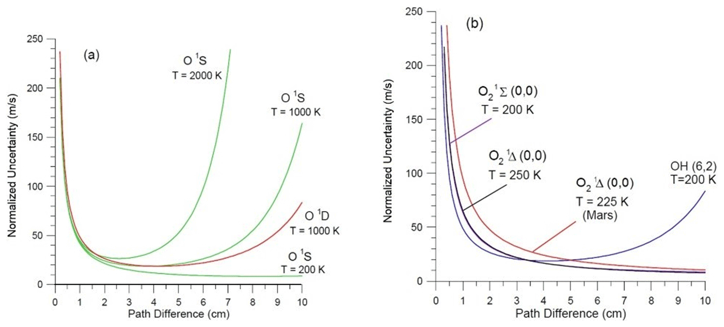
Figure 1 Normalized uncertainty plotted against D (0 to 10 cm) for several emissions. The O¹S emission is shown in green for three temperatures in panel (a).

Figure 2 Normalized uncertainty plotted against D (0 to 2.5 cm) for several emissions. The O¹S emission is shown in green for three temperatures in panel (a).

The ideal design of a general two-beam Doppler interferometer is optimized to have an effective path difference near the minima for a particular emission line. However, in some cases, such as for the instrument discussed in this paper, the physical size of the available components limits the effective optical path difference that can be achieved with the device. For BIDWIN, it is shown that the loss in sensitivity associated with this less-than-ideal effective path difference is compensated by the high SNR that can be achieved from the large throughput that is possible.

3 The Birefringent Doppler Wind Imaging Interferometer (BIDWIN)

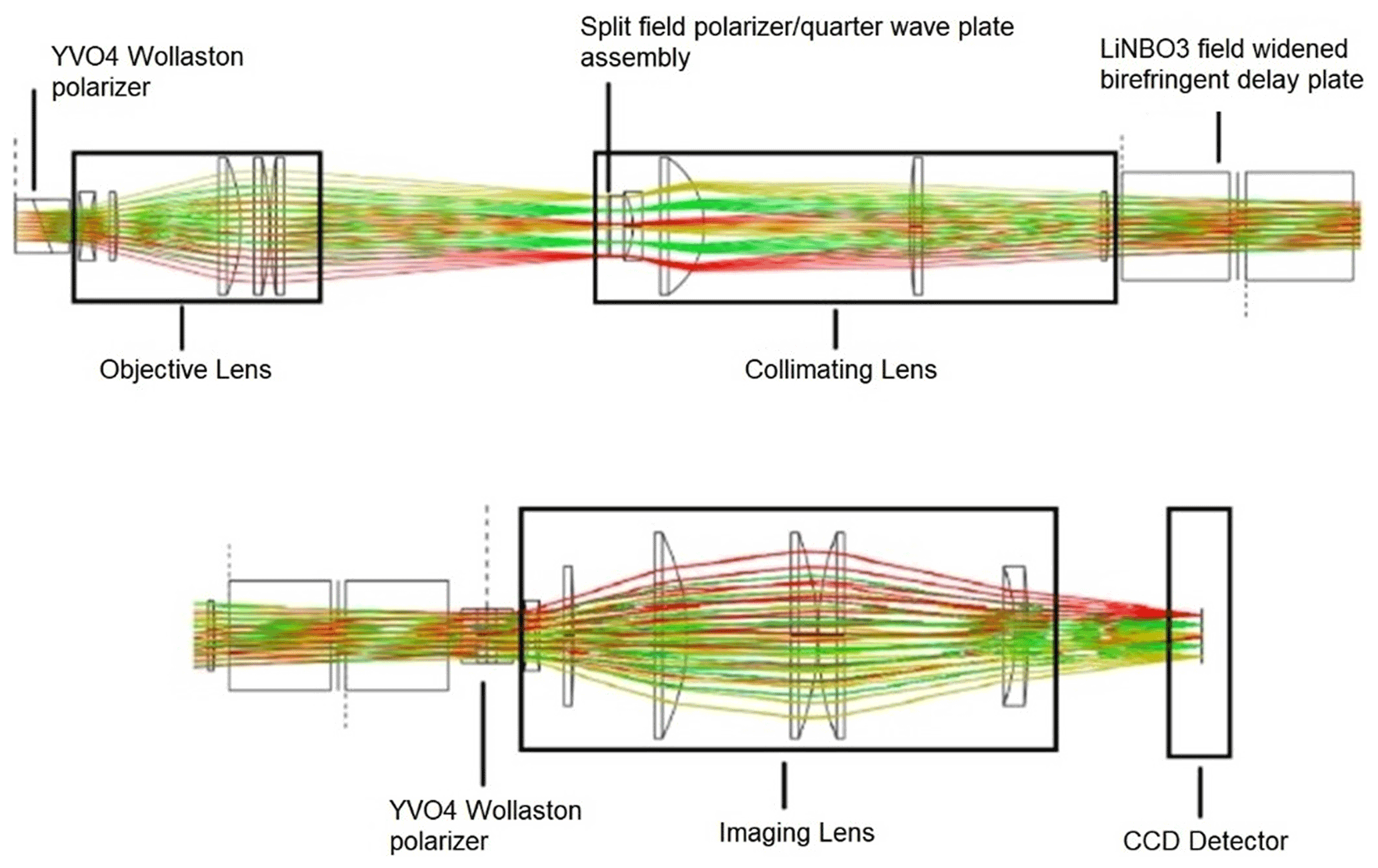
The optical layout of BIDWIN is depicted in Fig. 3, where the input is collimated light from the scene of interest. This light is incident on the first Wollaston prism, the aperture of which defines the entrance aperture of the optical system. The Wollaston splits the incoming radiation into two orthogonally polarized beams (vertical and horizontal). The objective lens located directly following the Wollaston forms orthogonally polarized images of the scene in the top frame and bottom frames of the split field polarizer conjugate to the field stop location. The polarization axes of the two sectors of the split field polarizer are oriented along the y and x axes corresponding to the orientation of the orthogonal polarizations produced by the Wollaston prisms. A quarter waveplate is attached to the bottom sector directly behind the polarizer with its optical axis oriented at 45^∘ to the x axis. Therefore, the light exiting from the top sector is linearly polarized, while the bottom sector is circularly polarized. An image of the field stop is passed through the field-widened delay plate as collimated light by the collimating lens. The delay plate introduces an optical path difference between the beams where the direction through the plate is mapped to position in the scene. The second Wollaston prism is positioned behind the field-widened delay plate and is rotated 90^∘ relative to the first Wollaston prism. After passage through this prism, the beam is split horizontally and is orthogonally polarized. The light exiting the Wollaston is collected by the imaging system which forms a four-quadrant image of the fringes of equal inclination, where each quadrant contains an identical image of the scene. As derived theoretically in the next few paragraphs, the four interference fringe images are phase stepped by $\mathit{\pi }/\mathrm{2}$ as idealized in Fig. 3.

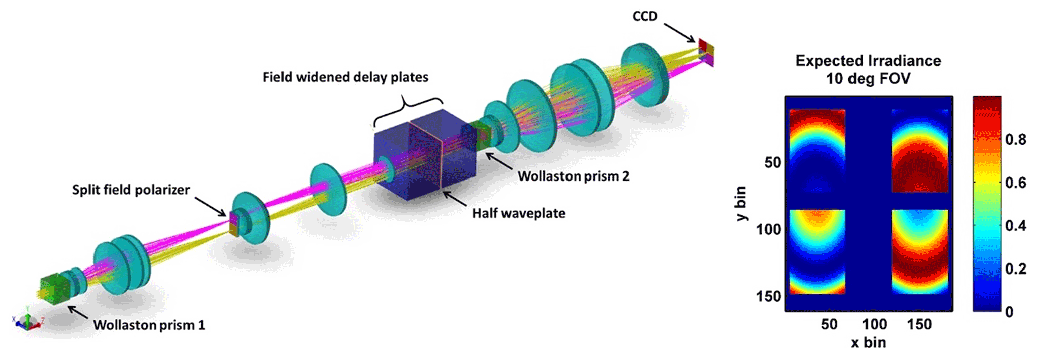
Figure 3 The prototype BIDWIN optical layout and simulated interference fringes at the detector.

The field-widened delay plate is constructed from two crossed equal-length uniaxial birefringent crystal slabs cut with the optical axis in the plane of the clear aperture with a half waveplate placed between them. The optical axis of the first slab is oriented at 45^∘ to the x axis and the second slab is 135^∘ to the x axis. The half waveplate is oriented with its optical axis along the y axis to ensure the polarization of the light incident on the second slab and the exiting light from the first slab are symmetric about the y axis. The optical path difference between the extraordinary and ordinary rays through the crystal depends on the incident angle θ as well as the azimuth ϕ of the incident light. In the case that the two slabs and the half waveplate are perfectly aligned, the optical path difference across the field of view is given to fourth order by Title and Rosenberg (1979):

$$\begin{array}{}\text{(5)}& \begin{array}{rl}\mathrm{\Delta }\left(\mathit{\theta },\mathit{\varphi }\right)& \approx {\mathrm{\Delta }}_{\mathrm{0}}\left[\mathrm{1}-{\displaystyle \frac{\mathrm{1}}{\mathrm{4}{n}_o^{\mathrm{2}}}}\left({\displaystyle \frac{n_e-n_o}{n_e}}\right){\sin }^{\mathrm{2}}\left(\mathit{\theta }\right)\right.\\ & \left.+{\displaystyle \frac{{\sin }^{\mathrm{4}}\left(\mathit{\theta }\right)}{\mathrm{8}{n}_o^{\mathrm{4}}}}+{\displaystyle \frac{\mathrm{1}}{\mathrm{8}{n}_o^{\mathrm{4}}}}\left({\displaystyle \frac{n_e-n_o}{n_e}}\right){\sin }^{\mathrm{4}}\left(\mathit{\theta }\right){\sin }^{\mathrm{2}}\left(\mathrm{2}\mathit{\varphi }\right)\right],\end{array}\end{array}$$

where ${\mathrm{\Delta }}_{\mathrm{0}}=l\left(n_e-n_o\right)$, and l is the total length of the two slabs. For most birefringent materials, the third term on the right-hand side is extremely small and the azimuthal dependence is negligible. In this case, the device is field widened, and the optical path difference varies slowly with incident angle. This configuration is extremely sensitive to misalignments or mismatches between the components and design errors. Exploring these sensitivities has been carried out using a Jones matrix framework that neglects Fresnel effects and Fabry–Pérot fringes but considers birefringent splitting and unwanted coupling between the e and o waves at the interfaces (Langille et al., 2020). In Sect. 4, we use this framework to examine the field-of-view sensitivity of the optimized design and compare modeled results to lab measurements. Here, we use the Jones matrix approach to present the measurement principle.

The incident light of the airglow can be regarded as unpolarized. Therefore, it is split into two orthogonally polarized beams by the first Wollaston prism. As a result, the top beam at the split field polarizer is vertically polarized and can be represented by the Jones vector ${\mathit{E}}_{\mathrm{t}}=\mathrm{1}/\sqrt{\mathrm{2}}\left[\begin{array}{l}\mathrm{0}\\ \mathrm{1}\end{array}\right]$, while the bottom beam is horizontally polarized and can be represented by the Jones vector: ${\mathit{E}}_{\mathrm{b}}=\mathrm{1}/\sqrt{\mathrm{2}}\left[\begin{array}{l}\mathrm{1}\\ \mathrm{0}\end{array}\right]$. For a perfectly aligned split field polarizer, the Jones matrix of the top polarizer is ${\mathbf{J}}_{\mathrm{t}}=\left[\begin{array}{ll}\mathrm{0}& \mathrm{0}\\ \mathrm{0}& \mathrm{1}\end{array}\right]$, while the Jones matrix of the bottom polarizer is ${\mathbf{J}}_{\mathrm{b}}=\left[\begin{array}{ll}\mathrm{1}& \mathrm{0}\\ \mathrm{0}& \mathrm{0}\end{array}\right]$. The Jones matrix of the attached quarter waveplate behind the bottom polarizer with a 45^∘ optical axis to the x axis is ${\mathbf{J}}_{\mathrm{q}}=\mathrm{1}/\sqrt{\mathrm{2}}\left[\begin{array}{ll}\mathrm{1}& i\\ i& \mathrm{1}\end{array}\right]$. The second Wollaston prism works as two polarizers when it splits the incident light into two beams deviate to the right (+x axis) and left (−x axis), respectively, and can be represented using two Jones matrices given by ${\mathbf{J}}_{\mathrm{r}}=\left[\begin{array}{ll}\mathrm{0}& \mathrm{0}\\ \mathrm{0}& \mathrm{1}\end{array}\right]$ and ${\mathbf{J}}_{\mathrm{l}}=\left[\begin{array}{ll}\mathrm{1}& \mathrm{0}\\ \mathrm{0}& \mathrm{0}\end{array}\right]$, respectively. The Jones matrix of the delay plate is represented by J_f. Applying the combined Jones matrices to the incident electric field produces output electric fields of the four frames at the charge-coupled device (CCD) detector location given by

$$\begin{array}{}\text{(6)}& E_{\mathrm{1}}=J_{\mathrm{r}}\cdot J_f\cdot J_{\mathrm{t}}\cdot E_t\end{array}$$

$$\begin{array}{}\text{(7)}& E_{\mathrm{2}}=J_{\mathrm{l}}\cdot J_f\cdot J_{\mathrm{t}}\cdot E_{\mathrm{t}}\end{array}$$

$$\begin{array}{}\text{(8)}& E_{\mathrm{3}}=J_{\mathrm{l}}\cdot J_f\cdot J_{\mathrm{q}}\cdot J_{\mathrm{b}}\cdot E_{\mathrm{b}}\end{array}$$

$$\begin{array}{}\text{(9)}& E_{\mathrm{4}}=J_{\mathrm{r}}\cdot J_f\cdot J_{\mathrm{q}}\cdot J_{\mathrm{b}}\cdot E_{\mathrm{b}}.\end{array}$$

In the case of perfect alignment, the Jones matrix J_f varies little with azimuthal angle ϕ of the incident light through the field-widened delay plates. To simplify the matrix J_f and obtain characteristic expressions for the intensity in each quadrant, we assume the incident plane lies along x axis and that the incident angles are small. Substituting into Eqs. (6) to (9) and then calculating the average intensity for each beam, the samples in each frame are given by

$$\begin{array}{}\text{(10)}& I_{\mathrm{1}}={\displaystyle \frac{\mathrm{1}}{\mathrm{4}}}\left[\mathrm{1}+\cos \left({\mathit{\varphi }}_{\mathrm{1}}\right)\right]\end{array}$$

$$\begin{array}{}\text{(11)}& I_{\mathrm{2}}={\displaystyle \frac{\mathrm{1}}{\mathrm{4}}}\left[\mathrm{1}+\cos \left({\mathit{\varphi }}_{\mathrm{2}}+\mathit{\pi }\right)\right]\end{array}$$

$$\begin{array}{}\text{(12)}& I_{\mathrm{3}}={\displaystyle \frac{\mathrm{1}}{\mathrm{4}}}\left[\mathrm{1}+\cos \left({\mathit{\varphi }}_{\mathrm{3}}+{\displaystyle \frac{\mathit{\pi }}{\mathrm{2}}}\right)\right]\end{array}$$

$$\begin{array}{}\text{(13)}& I_{\mathrm{4}}={\displaystyle \frac{\mathrm{1}}{\mathrm{4}}}\left[\mathrm{1}+\cos \left({\mathit{\varphi }}_{\mathrm{4}}+{\displaystyle \frac{\mathrm{3}\mathit{\pi }}{\mathrm{2}}}\right)\right],\end{array}$$

where ϕ_i $\left(i=\mathrm{1},\mathrm{2},\mathrm{3},\mathrm{4}\right)$ is the background phase in each quadrant determined from Eq. (5). For each incident angle θ and azimuth ϕ, ϕ_i has a different value in the four frames and varies across the field of view, resulting in a variation of the phase steps across the scene. In practice, the transmission and the instrument visibility will also vary across the image in each quadrant. If we assume the relative intensities and the instrument visibilities in various measurements are fixed, for a single point, the intensity $I_i^j$ of the ith step (frame) in the jth measurement can be modeled as

$$\begin{array}{}\text{(14)}& I_i^j=K_{\mathrm{i}}{I}_{\mathrm{0}}^j\left[\mathrm{1}+U_{\mathrm{i}}{V}^j\cos \left({\mathit{\varphi }}^j+{\mathit{\phi }}_i\right)\right],\end{array}$$

where $I_{\mathrm{0}}^j$ is the mean intensity, and V^j is the line visibility. In practice, the thermal drift of the optical path difference due to the dependence of the birefringence on temperature as well as variations in length due to thermal expansion and contraction of the components will introduce a time-varying phase shift not shown in Eq. (14). A slight phase shift (Eq. 2) associated with a Doppler shift in a moving source can be extracted from the samples using general fringe analysis algorithms if the relative intensities K_i, instrument visibilities U_i, phase steps φ_i $\left(i=\mathrm{1},\mathrm{2},\mathrm{3},\mathrm{4}\right)$ and the thermal drift are known. Therefore, these parameters must be carefully calibrated. This is achieved by performing measurements of light from a calibration source emitting a spectral line close to that of the target emission. Observations of the calibration source must be performed frequently enough to track the thermal drift.

While a full analysis of stray light is outside the scope of this work, another important feature of the BIDWIN approach is that each quadrant images the same field. Therefore, the background or scattered light from the field will be unmodulated and appear as a constant offset for the corresponding bins in each quadrant. In this case, the fringe phase will not be affected.

4 Prototype instrument design

4.1 Overview

The prototype BIDWIN instrument has been developed for lab performance evaluation and ground-based field testing. Due to the chromatic dispersion of the waveplates in the system, the instrument can only be optimized for operation at a single wavelength. Another important constraint on the design is the acceptable range of possible effective path differences for a compact field-widened birefringent delay plate. This is determined by two factors. First, the magnitude of the birefringence and the availability of large-format high-quality crystals limits the fixed path difference to the range of 0 to 2 cm. Second, the overall sensitivity of the device to the measurement of Doppler winds is optimized when the normalized wind uncertainty reaches a minimum as shown in Figs. 1 and 2. From these figures, we see that only the O¹S and O¹D emissions have normalized uncertainty minima below D=5 cm. Both emissions have similar emission rates when observed from the ground; however, the O¹S emission at 557 nm corresponds to a layer from 95 to 110 km, whereas the O¹D emission corresponds to a layer between 150 and 300 km. In addition, the dynamical motions in the upper layer result in LOS Doppler winds that are on the order of a few hundred m s⁻¹, whereas typical motions in the lower layer result in LOS Doppler winds on the order of 10 m s⁻¹.

The prototype version of the instrument is optimized to target the O¹D emission at 630 nm. Measurements with uncertainties better than ±5 m s⁻¹ are needed to advance our scientific understanding of neutral motions at these heights. Representative emission rates observed at the ground from the O¹D emission varies through the course of a day and has a seasonal dependence. However, typical emission rates are expected to be near 100 R (R: Rayleighs) for ground-based observations. Optimization of the instrument for 630 nm also allows for lab testing and characterization work to be performed using a stabilized He–Ne laser emitting 632.8 nm. This is ideal since it provides a high-SNR stabilized source with a fixed polarization. The overall requirements that are used to optimize the prototype design are listed in Table 4.

Table 4 Primary science requirements for the BIDWIN prototype instrument.

4.2 Interferometer design

The primary practical considerations driving the interferometer design are the effective path difference, the SNR and the resulting sensitivity for the measurement of Doppler winds. Several additional criteria were also used to constrain the design of the field-widened birefringent delay plate. These include the cost, availability and workability of large-format high-quality birefringent crystals, the magnitude of birefringence and the thermal stability of the design. LiNBO₃, YVO₄ and CaCO₃ were investigated. YVO₄ and CaCO₃ achieve a larger path difference compared to lithium niobate due to their larger birefringence; however, large-aperture YVO₄ crystals are difficult to obtain, and CaCO₃ is extremely difficult to work with in practice due to its softness. On the other hand, large-format LiNBO₃ crystals are readily available, allowing for a large-throughput device to be constructed. All these crystals have strong thermal sensitivities, on the order several fringes per degree Celsius change in temperature, resulting in associated wind variation of ∼10³ to ∼10⁵ m s⁻¹. Therefore, the thermal drift of the instrument must be carefully tracked by making periodic measurements of a calibration source and the interferometer must be placed in a thermally controlled enclosure for the field implementation. Thermally compensated designs are also possible (Hale and Day, 1988) and are under consideration; however, this aspect is not considered for the design presented in this paper.

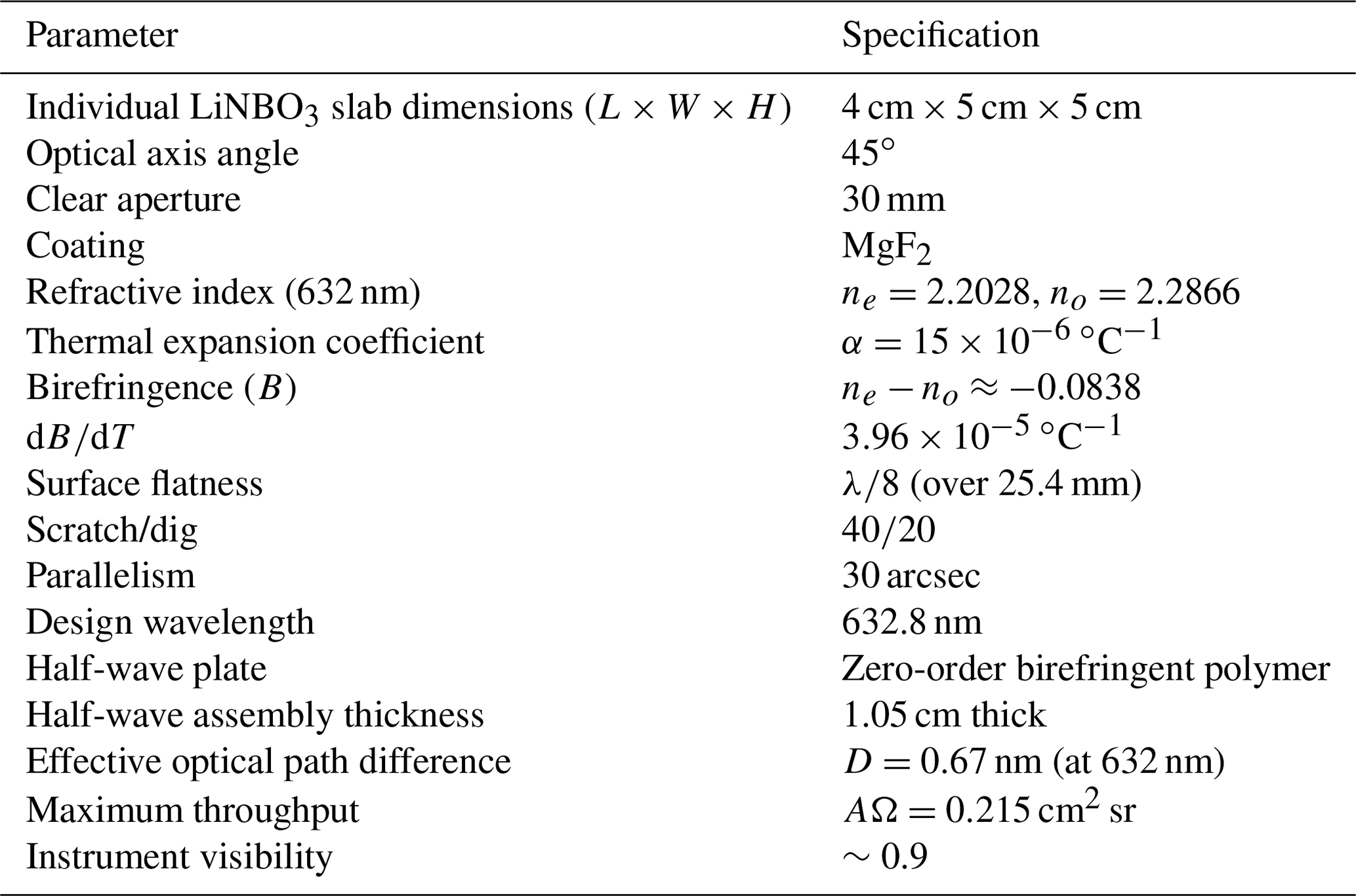
The specifications for the BIDWIN prototype interferometer are shown in Table 5. The interferometer is constructed from two equal-length slabs of LiNBO₃ that have dimensions 4 cm × 5 cm × 5 cm. The manufacturer guaranteed the optical quality (surface flatness, scratch dig, etc.) across a clear aperture of 30 mm centered on the optical axis of the slabs. The true zero-order half-wave plate utilized in the system is a 25.4 mm clear aperture element constructed from a birefringent polymer cemented between two slabs of BK7 manufactured by Meadowlark optics. The thickness of the half-wave plate element, including the mounting, is ∼1.05 cm. It is optimized for operation at 632.8 nm and has a thermal dependence of the retardance of ∼0.15 nm ^∘C⁻¹ and an angular sensitivity of $<\mathrm{1}\mathit{\%}\pm \mathrm{5}$^∘. The effective path difference of the interferometer is D=0.67 cm.

Table 5 Specifications of the lithium niobate slabs used to construct the field-widened birefringent delay plate.

The maximum throughput that can be obtained with the device is fixed by the geometry of a solid block of glass as shown in Fig. 4. The figure shows an incident ray passing through a simple rectangular slab of birefringent material. To achieve as large a signal as possible, the instrument should be designed so the product AΩ is as large as possible, within whatever restrictions exist. The usual way to send light through an interferometer is to place a telescope in front that defines the field of view and passes a well-defined collimated beam through the interferometer with an image of the entrance aperture located at the center of the device.

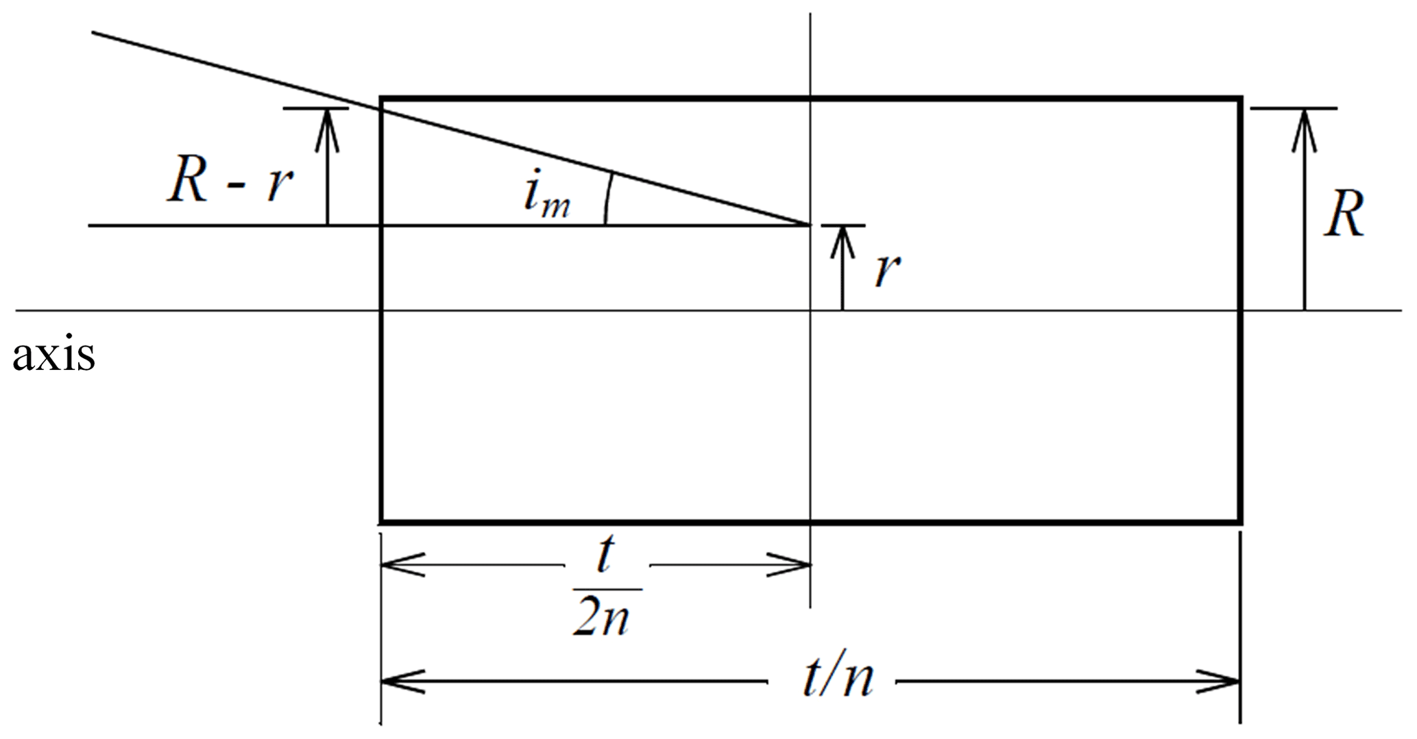
Figure 4 The rectangle represents the interferometer of thickness t. A ray enters near the edge at incident angle i_m and reaches midway at distance r above the axis. R is the available radius at both ends of the interferometer. The thickness is shown as air equivalent, $t/n$, where n is the refractive index.

Assuming a square field of view and a circular entrance aperture, the product AΩ, called the étendue, is given by

$$\begin{array}{}\text{(15)}& A\mathrm{\Omega }=\left(\mathit{\pi }{r}^{\mathrm{2}}\right){\left[\left({\displaystyle \frac{R-r}{t/\mathrm{2}n}}\right)\right]}^{\mathrm{2}},\end{array}$$

where R and r are the clear extent of the slab and the radius of the image of the aperture respectively. The maximum AΩ is achieved when the image of the entrance aperture midway through the interferometer is half the diameter of the available area at the ends of the interferometer. Considering the full length of the assembly (t=9.05 cm), substituting R=15 mm into Eq. (15) and assuming n∼2.2 gives a maximum possible throughput of 0.235 cm² sr. This corresponds to a maximum of axis angle through the clear aperture of roughly 20.03^∘. To mitigate the potential for clipping the housing, we limit this to 20^∘, resulting in a solid angle of the square field of view of 0.122 steradians and a corresponding throughput of AΩ=0.215 cm² sr for the field-widened element.

A picture of the assembled prototype is shown in Fig. 5a. The fully assembled element is roughly 10 cm in length including the mounting. The optical path variation as a function of incident angle for the device is shown in Fig. 5b. The extent of the field widening is clear – less than 3.5 fringes enter the field of view with incident angles of 20^∘. As an example, the simulated interference image produced using this device as the delay plate in the in the BIDWIN optical system assuming a range of off-axis angles of 10^∘ is shown in Fig. 5c. In this simulation, the detector is taken to have 250 × 250 bins, and ideal polarization selection by the Wollaston prisms is assumed.

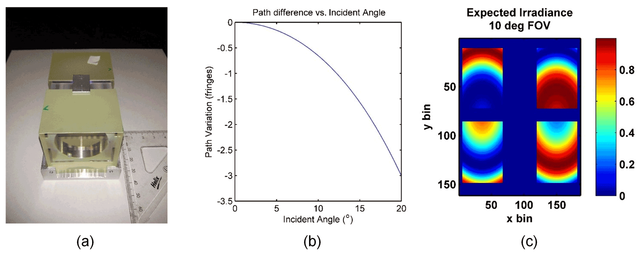
Figure 5 The assembled LiNBO₃ field-widened delay plate (a), optical path variation with incident angle (b) and a simulated four-quadrant image assuming the configuration discussed in Sect. 3 (c).

The phase variation across the image of the scene and the associated quadrature between the samples in the image is shown in Fig. 6a–c. The upper left panel shows the phase across the top quadrant and the upper right panel shows the phase variation across the bottom quadrant. The associated phase quadrature is shown in the bottom left panel. Note that there are several “strips” across the image that have zero phase quadrature. The four-point algorithm cannot be applied to these samples, which results in enhanced wind errors within these regions. The expected wind uncertainty calculated using Eq. (4) is shown in Fig. 6e as a function of the SNR. Here, we observe that an SNR > 700 is required to achieve wind precisions of <5 m s⁻¹. Therefore, we examined the sensitivity across these strips by performing Monte Carlo simulations assuming Poisson noise and an SNR = 700. Large wind errors are observed in the zero-quadrature regions as shown in Fig. 6d. This effect is enhanced as the field of view is increased; therefore, care must be taken to properly identify and characterize these regions during data processing. However, the presence of these zero-quadrature regions also provides an opportunity to simultaneously sample the intensity at several positions in the scene. The potential application of this feature for a potential limb-viewing satellite version of the instrument is presented in Sect. 6.

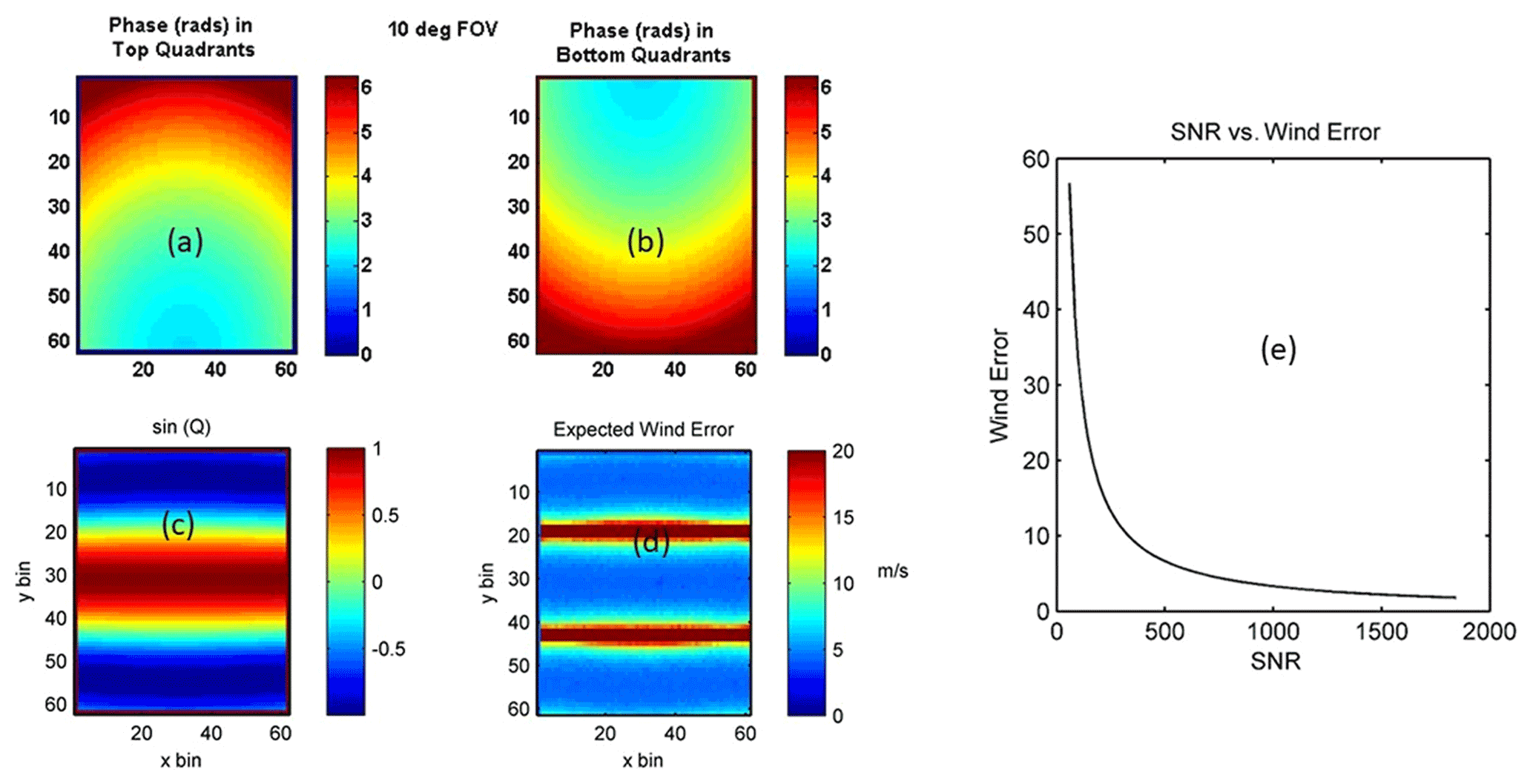
Figure 6 The expected phase variation in the top (a) and bottom (b) quadrants of the BIDWIN instrument and the phase quadrature between samples (c) assuming a 10^∘ field of view. The expected wind uncertainty (d, e) assuming the instrument characteristics listed in Table 5 and the signal characteristics listed in Tables 4 and 2.

As a simple example, we estimate the expected SNR from Eq. (3) as SNR $\sim \sqrt{S}$ and determine the integration time that would be required to achieve wind precisions <5 m s⁻¹ using the prototype. For this example, we assume ground-based observations and take E_o=100 R. We also substitute realistic instrument parameters τ∼0.1, η∼0.9, AΩ=0.215 cm² sr and assume that the field is sampled into 100 bins. Furthermore, we make the conservative estimate that roughly 25 % of the field may lie within the zero-quadrature regions that are unusable for wind measurements. In this case, an integration time of 425 s would be required to achieve an SNR ∼ 700 (and a wind precision of <5 m s⁻¹). This integration time is too long to be useful; therefore, the current prototype cannot be used for ground-based imaging of the wind field. However, in the case of single-point wind measurements, an SNR ∼ 700 can be reached with an integration time of 4.25 s, which is much more practical. Note that if one obtained a crystal with high quality across the full 5 cm aperture, the maximum throughput can be significantly increased. In fact, crystals as large as 12 cm × 100 mm × 100 mm are readily available, which would allow a device with a throughput more than 4 times that of the prototype to be realized. In this case, the imaging aspect will also be feasible; however, the cost of manufacturing the slabs also increases and the larger crystals must be accommodated by larger imaging optics. The design of a proposed field instrument is discussed further in Sect. 6.

4.3 The imaging system

The side-view ray trace through the BIDWIN optical system is shown in Fig. 7. As discussed in the previous section, the throughput of an ideal system is limited by the maximum throughput that can be provided by the delay plate. However, in the case of the breadboard instrument, it was the size and availability of large-format Wollaston prisms that limited the maximum throughput. The prisms utilized in the breadboard system are constructed from two YVO₄ wedges. The wedges are designed to provide a split angle of ∼9.29^∘ (at 632.8 nm) between the two orthogonal polarizations exiting the Wollaston. The objective lens is designed to accept an input field of view of 4^∘ square and the 10 mm diameter pupil of the prism located directly in front of the objective lens defines the entrance aperture of the optical system.

Figure 7 The BIDWIN optical design (side-view ray trace).

The objective lens was optimized such that the output beam is approximately telecentric, which minimizes the incident angle at the waveplate/split field polarizer location. This is done to reduce the impact of the incomplete polarization selection of off-axis rays at the polarizer and slight shifts in the retardance of the quarter waveplate due to the angular dependence of the retardance. The collimating lens is designed to pass a collimated image of the field stop through the field-widened birefringent delay plate. The collimating lens also forms an image of the entrance aperture midway between the birefringent delay plate. The imaging lens is optimized to correct for aberrations and focus the collimated beams onto the detector. All the lenses are spherical and are constructed from BK7 and have been anti-reflection coated for visible wavelengths.

A comparison between the interference fringes simulated using Zemax optical design software (upper panels) and the observed fringes (lower panels) in the lab is shown in Fig. 8. Three examples are shown. The first example (Fig. 8a and d) shows the case of ideal alignment between the components. We observe less than one fringe in the field of view and the images are phase stepped in 90^∘ increments. Because of the breadth of the fringe, its form in the lower panels is more difficult to see. The shape of the field stop that is located near the split field polarizer is observed in the lower panel and the edges of the split field polarizer can also be seen. In the second example, the back crystal has been rotated by 10^∘. This misalignment introduces high-contrast hyperbolic fringes as well as a set of low-amplitude parasitic fringes. The parasitic fringes are the result of misalignment relative to the half-wave plate and are removed in the third example by rotating the half-wave plate by 5^∘. All three cases agree extremely well with the simulated fringes and serve to demonstrate the sensitivity to misalignment as well as the overall imaging quality of the optical system.

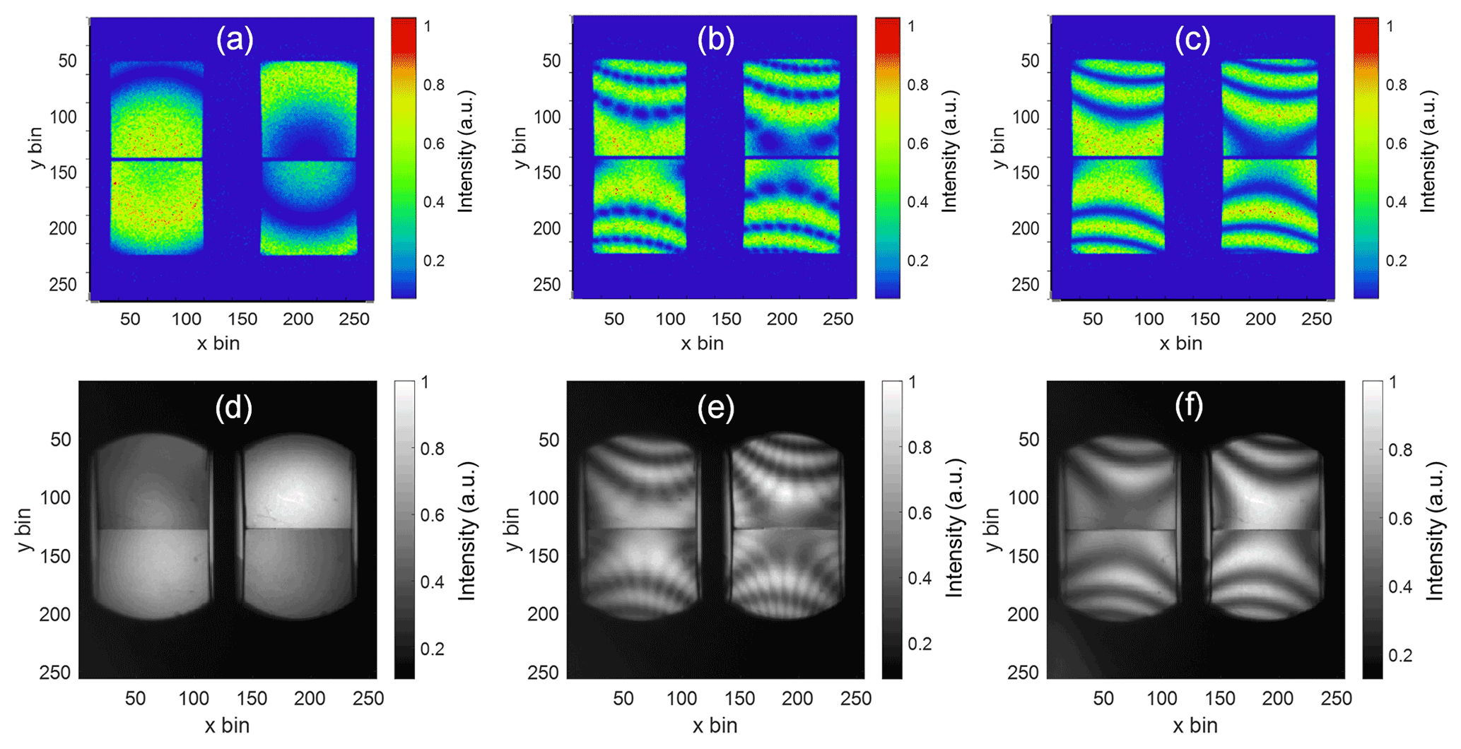
Figure 8 Comparison between the simulated (a–c) and observed (d–f) interference fringes for the case of perfect alignment (a, d), a 10^∘ misalignment between the lithium niobate slabs (b, e) and the same as in panels (b, e) with the half-wave plate rotated by 5^∘ to eliminate the low-amplitude parasitic fringes.

5 Lab performance

5.1 Setup

The BIDWIN prototype instrument was assembled at the Atmospheric and Space Physics Lab at the University of New Brunswick. The system used to produce a predictable gradient in the LOS wind field within the field of view of the instrument is shown in Fig. 9. Light incident from a He–Ne laser is diffused and passed through a beam splitter to illuminate a retroreflective disk that was oriented at an angle of 45^∘ to the optical axis. The disk was attached to a chopper and controller system with which the rotation rate of the wheel was accurately controlled. Light retroreflected from the disk is reflected by the beam splitter and collimated before being collected by the BIDWIN entrance optics. Light emitted from the He–Ne laser is only partially polarized with a narrow range of polarizations near some specific angle of polarization close to the direction of the y axis. Therefore, a polarizer oriented at 45^∘ to the x axis was placed in front of the system to ensure the two beams split by the first Wollaston prism are equal in intensity. This polarizer is not required when observing the unpolarized airglow. An Apogee U47 CCD with a resolution of 256 × 256 on 2 × 2 binning is used for imaging. The imaging optics part of the lab prototype was configured slightly different from Fig. 3. A folding mirror and lens are used to reimage the primary interference fringe image to ensure the four frames match the size of the CCD that was available for lab testing. In addition, the field of view of the optical system, set by an intermediate stop in the wind wheel system, is a 4^∘ circle instead of a square field of view.

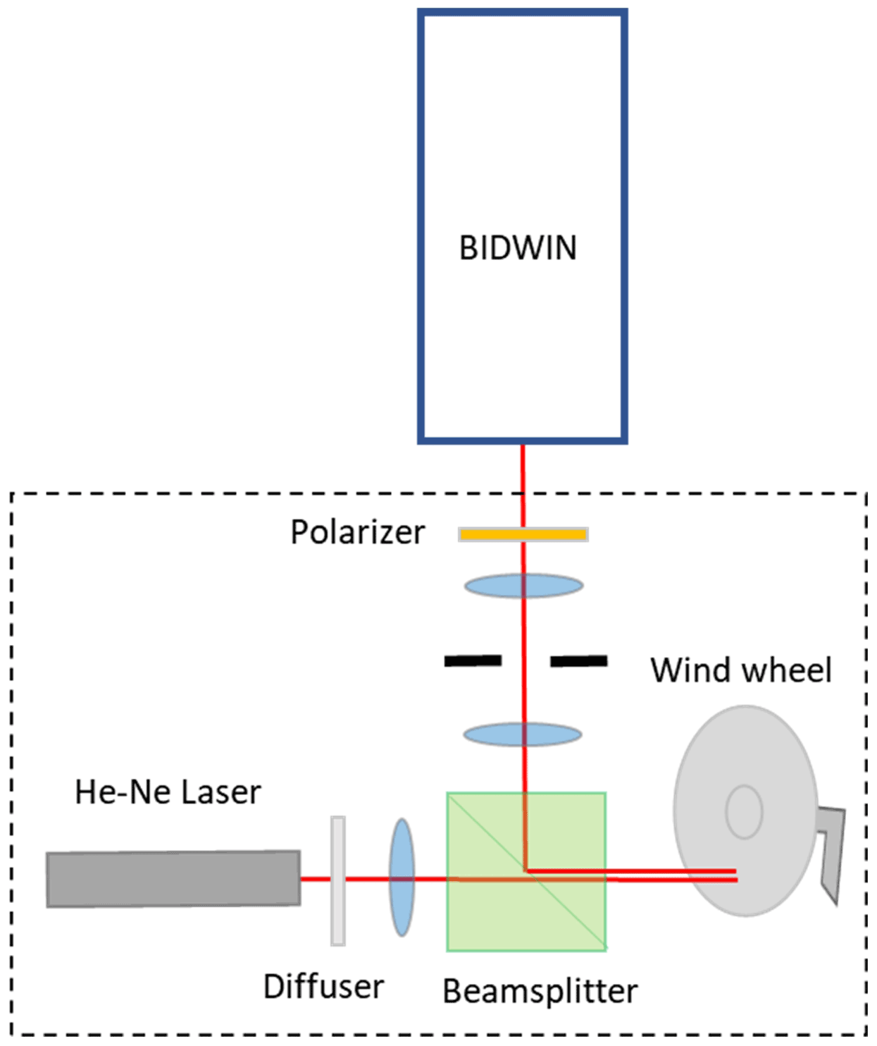
Figure 9 Schematic of the system used to produce a predicable gradient in the LOS wind field within the field of view of the instrument in the lab.

5.2 Characterization and calibration

The calibration of the fringe parameters as discussed in Sect. 2 can be achieved by scanning the wavelength of a suitably isolated spectral emission line, scanning fringes through temperature variations (i.e., using the thermal dependence of the glass properties to change the path) or by rotating the field-widened delay plates (Gault et al., 2001) and sampling the interference pattern at each step. In our experiment, scanning the wavelength of the frequency stabilized 632.8 nm He–Ne laser was not possible, so we utilized the strong thermal dependence of the lithium niobate slabs to scan the optical path.

Because of the thermal sensitivity of the field-widened delay plates, a scan in the optical path of almost two fringes can be performed by letting the system respond to the variation of the lab temperature over roughly 30 min as shown in Fig. 10. It is obvious that the frequency of the cosine curve is changing during the scan, suggesting that the variation of the lab temperature is not linear. The least mean square (LMS) algorithm initially developed by Ward (1988) and refined by Kristoffersen (2019) and Kristoffersen et al. (2021) to simultaneously determine both the phase steps associated with sampling a fringe and the fringe parameters of the emission can be applied. In this case, the instrument fringe parameters from every bin in each quadrant must be characterized before standard fringe analysis techniques can be used. This characterization includes determining the relative phases of the four bins viewing the same segment of the scene, the φ_i, the instrument visibility, U_i and the relative responsivity, K_i. An elegant way of visualizing this process is through Lissajous mapping (Yan et al., 2021). The measured intensities of two quadrants during a thermal scan of BIDWIN are used to fill the 2π phase space of a fringe and in a least-mean-square sense determine the ellipse associated with this measurement set. Using the parameters of the ellipse, K_i, U_i and φ_i can then be calculated. Applying this algorithm to all the points in the field of view, we can acquire two-dimensional images of the calibrated fringe parameters: K_i, U_i and φ_i. The fringe parameters obtained using this approach are shown in Fig. 11.

Figure 10 The intensities of the center points measured by the thermal scanning of BIDWIN.

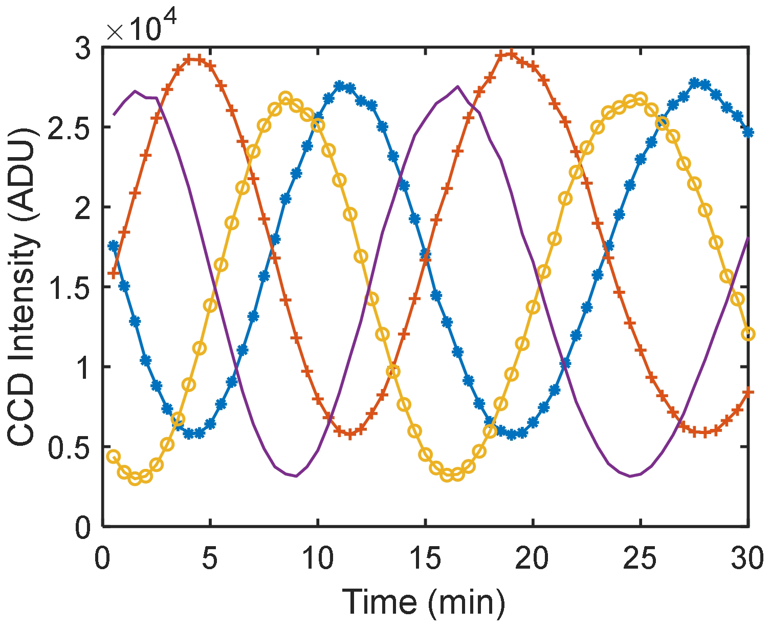
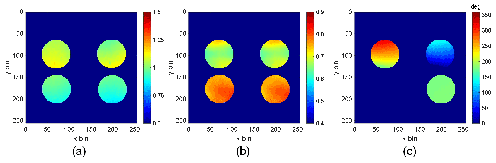
Figure 11 The calibrated parameters over the field of view of BIDWIN: (a) relative intensities K_i; (b) instrument visibilities U_i; (c) phases φ_i relative to the first quadrant.

Before applying these calibration parameters to the observations, the phase order of four quadrants must also be determined. Ideally, the steps should be in 90^∘ increments. According to the Jones matrix model, the phase steps come from the four combinations of polarizers and waveplate. Therefore, we can match those combinations with the four quadrants on the detector by observing the intensities of the four quadrants after removing the field-widened delay plates. After the phase order determination, it was found that the quadrant of the first phase step is the left bottom one because of the added folding mirror and lens in the imaging system. Flat-field images were also obtained using this configuration by placing a polarizer oriented at 45^∘ at the position of the field-widened delay plates.

Figure 11 shows the results of the K_i, U_i and φ_i calibration. In Fig. 11a, the relative intensities of the top quadrants are slightly higher than the bottom quadrants. Besides the misalignment of the optical train, a possible source of this variation is the angular error of the polarizer in front of the system, which should be oriented at exactly 45^∘ to ensure the two split light beams from the first Wollaston prism are equal. The instrument visibilities are mainly affected by features of the lithium niobate plates, such as the surface flatness and uniformity. As is shown in Fig. 11b, unlike the scanning mirror but similar to the segmented mirror Michelson interferometers, the visibilities of the four quadrant samples exhibit strong differences. It is obvious that the top and bottom light beams propagate through different parts of the crystal and result in different visibilities. In our experiment, we found that the visibilities of the four quadrants varied upon translation of the lithium niobate plates perpendicular to normal incidence. This suggests some spatial path variations that are larger (or smaller) for different regions of the crystal surface. For the lab measurements, this leads to a less-than-ideal instrument visibility that is smaller than the expected (U∼0.5 rather than 0.9). This was partially compensated by reducing the aperture area to increase the instrument visibility to ∼0.7, as shown in Fig. 11b. From Eqs. (3) and (4), these adjustments demand a proportional increase in the SNR that is required to achieve wind precisions of <5 m s⁻¹. The field implementation that is discussed in Sect. 6 will be manufactured with better surface quality to achieve U∼0.9.

The calibrated phases shown in Fig. 11c are the phase differences of the four quadrants relative to the first one (lower left quadrant which necessarily will have a relative phase of zero). The phase differences between the two horizontally split quadrants of top and bottom should be exactly 180^∘. However, the phase differences between the top and bottom quadrants vary across the field of view. This is because the upper and lower beams separated by the first Wollaston prism form identical images of the scene within the top and bottom quadrants of the split field polarizer. The field from the top and bottom quadrants is then passed as collimated light through the field-widened delay plates – mapping direction through the plate to position on the field stop. Therefore, the phase in the upper quadrant is mapped to position (and associated direction through the plate) in the top portion and the phase in the lower quadrant is mapped to position in the bottom quadrant. The resulting phase steps between the upper and lower neighboring quadrants have a vertical distribution in the field of view, and the sin (φ₁−φ₂) is shown in Fig. 12a.

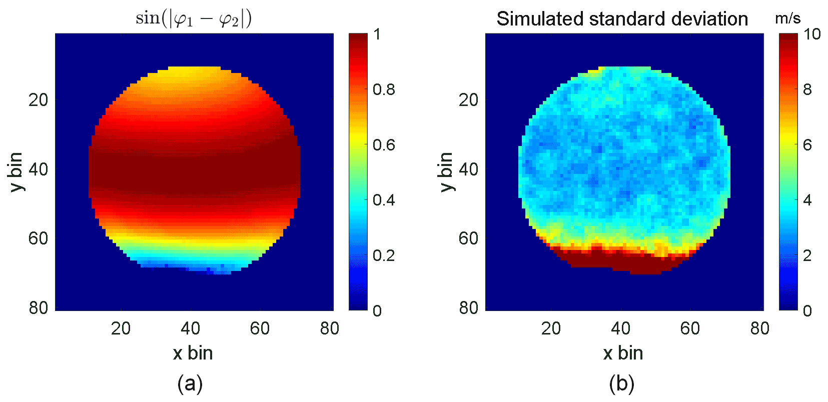
Figure 12 The sine value of the phase steps between φ₁ and φ₂ and the simulated standard deviation using calibrated parameters: (a) the sin (φ₁−φ₂) distribution in the field of view; (b) simulated standard deviation in retrieved wind.

The ideal phase step for the four-point algorithm generally used for fringe sampling is 90^∘ (Shepherd, 2002); relative phase steps deviate increasingly from this ideal with increasing incident angle (field of view). This results in larger uncertainties in the retrieved Doppler shifts as discussed in Sect. 4 (see Kristoffersen et al., 2021, for a detailed discussion of the effect variations in phase steps have on fringe parameter determinations). The simulated uncertainty distribution for the current configuration was simulated using the calibrated K_i, U_i and φ_i using a Monte Carlo method. In the simulation, shot noise was added to the signal with a SNR of 1000. The result is shown in Fig. 12b. Observe that bins close to the top and bottom edges have greater uncertainties. Therefore, the region of the field of view that can be used to achieve a wind precision less than 5 m s⁻¹ is only slightly restricted here.

5.3 Lab wind measurements

Two sets of wind measurements were conducted in the lab to examine the performance of the BIDWIN system. The first experiment is a single-point wind measurement. This involved observing a specific point on the wind wheel and rotating the wheel at different rates so that a series of velocities was observed. This experiment tested the Doppler shift measuring capacities of BIDWIN without including the imaging capability. The second experiment is a two-dimensional wind measurement which was performed by imaging an area of the wind wheel when it is rotating at a certain specified frequency.

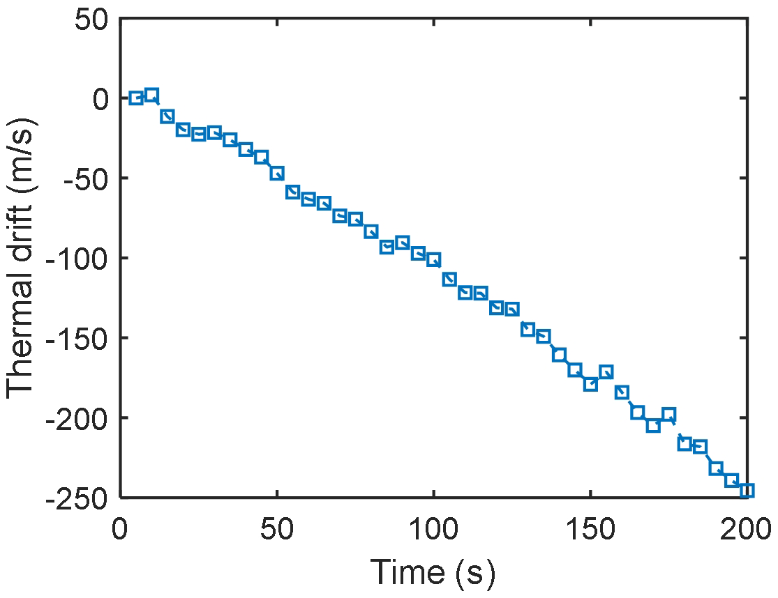
To make a wind measurement, phase measurements of the rotating wheel and stationary wheel are required. The phase measurements with the stationary wheel provide the zero-wind background phase. Wind measurements are determined from the phase difference between this phase and the phase of the rotating wheel. Without a good thermal enclosure, frequent measurement of this background phase is essential for these experiments because the system is highly sensitive to temperature (the thermal drift corresponds to roughly 1.25 m s⁻¹ per second in the experiment; see Fig. 13). This drift can dominate the wind determinations unless carefully monitored and calibrated. In our experiment, we removed this phase by linear fitting. The measurement sequence for Doppler wind measurement is similar to the measurement approach for MIADI, in which the zero-wind image was taken after each wind measurement (Langille et al., 2013b). The time of each wind measurement was recorded, and the background phase of that moment could be interpolated.

Figure 13 Thermal drift of BIDWIN over a 200 s interval using He–Ne laser as the source.

For the single-point experiment, the distance from the wheel center to the center point of the narrow field of view was 4 cm. Phase determinations were made using the 30-pixel by 30-pixel region illuminated on the CCD, resulting in an irradiance SNR of ∼1000. The frequency of wheel rotation was adjusted incrementally from 10 to 120 Hz in steps of 10 Hz to provide a range of line-of-sight speeds to evaluate the wind determination. The wind velocity measured using BIDWIN is plotted versus the wind wheel velocity determined from the rotation rate in Fig. 14. The straight blue line is the expected velocity. The red circles are the average measured velocity of nine measurements and the error bars are the standard deviations. The average standard deviation of the 12 points is 4.53 m s⁻¹, which confirms that upper atmospheric Doppler wind measurements with a precision of 5 m s⁻¹ are feasible using this technique if high SNR is achievable.

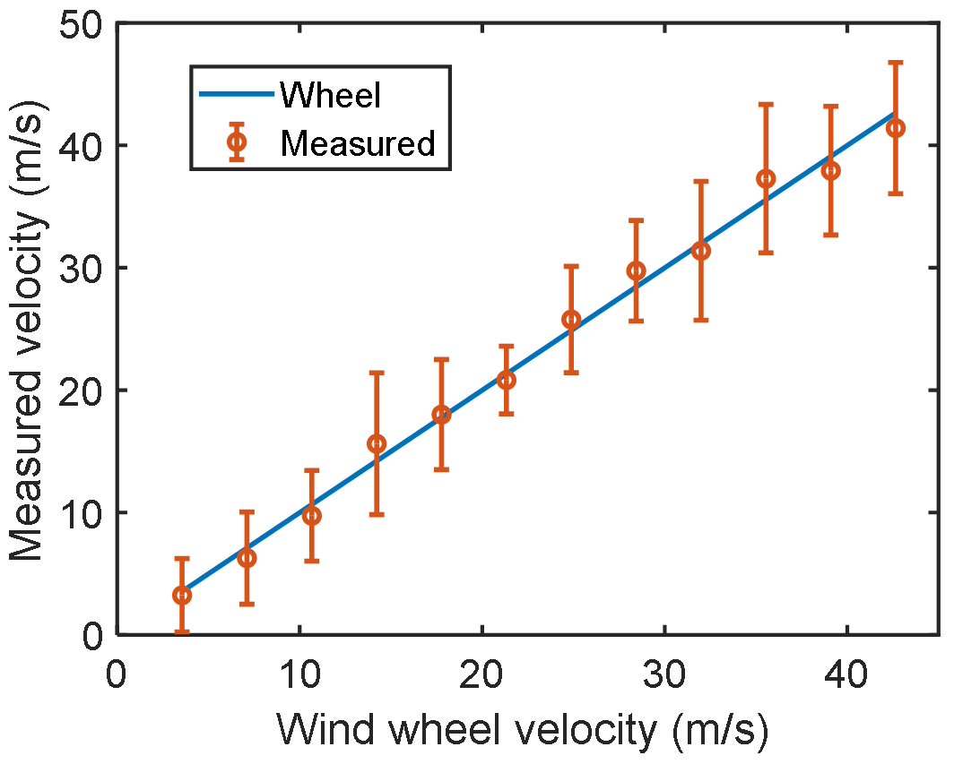
Figure 14 Measured wind velocity for single-point measurements is plotted versus the wind wheel velocity.

The imaging capability was examined by illuminating a 2 cm diameter circular area centered 4 cm from the center of the retroreflecting disk. The position of each pixel relative to the center of the wind wheel was determined by imaging a grid scale printed on a circular transparent plastic sheet which had a same size as the disk. Six measurement sets were taken using a rotation frequency of 105 Hz. The exposure time was adjusted to get a SNR of 1000 by averaging neighboring pixels. Because all bins in the wind field are measured simultaneously, there is no thermal drift across the field of view; therefore, the thermal drift calibration for one point can be applied to the whole field while removing the background phase. The expected wind field is shown in Fig. 15a and the average of the six BIDWIN Doppler wind field measurements is shown in Fig. 15b. The velocity gradients of the two wind images are consistent in shape and in magnitude. Some spatial variability is observed that does not track the gradient; however, it is possible that this is associated with contamination from light scattered from the disk that is not perfectly retroreflected due to spatial variations across the disk.

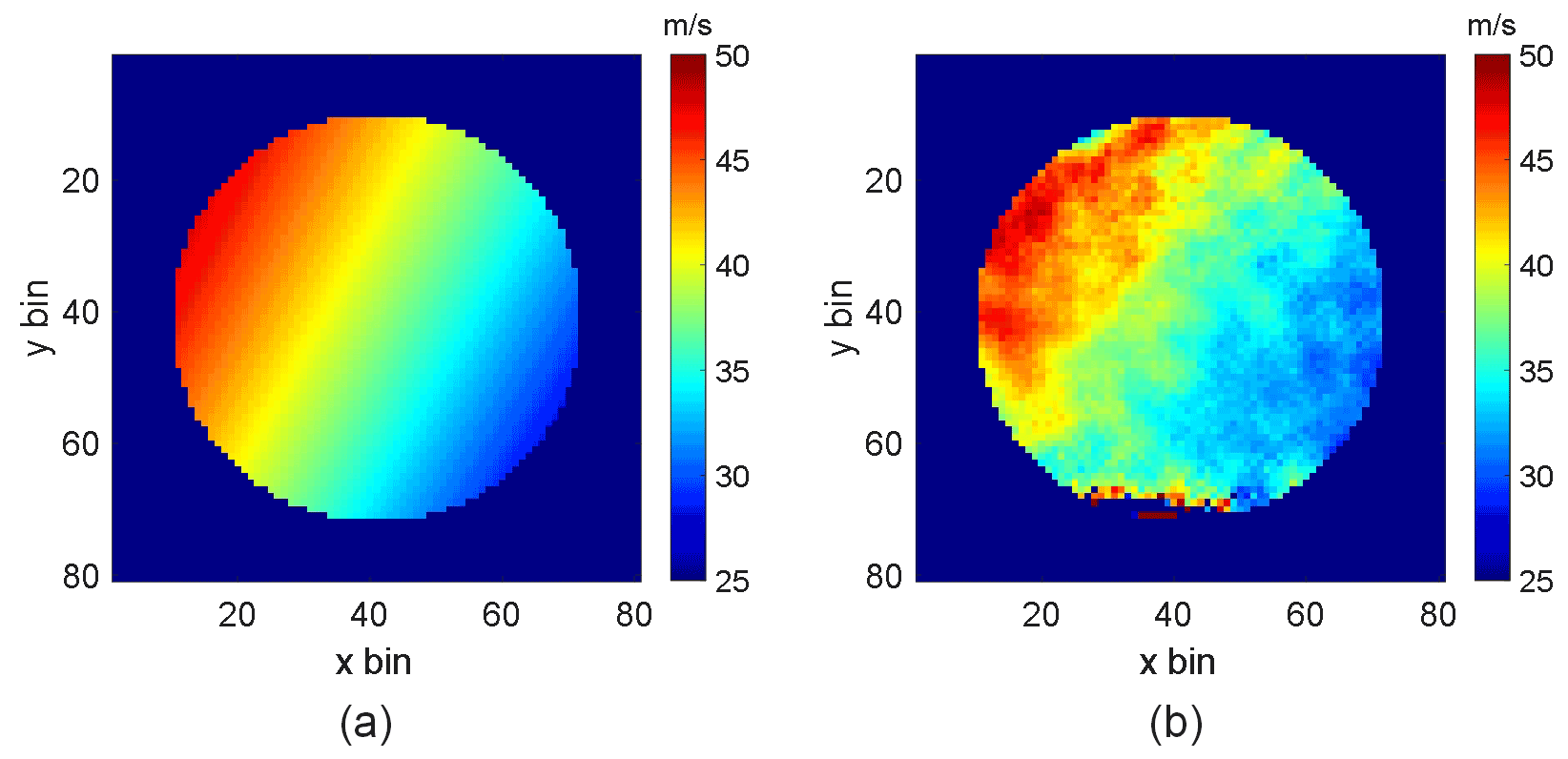
Figure 15 The expected and measured two-dimensional wind field across the wind wheel: (a) expected wind field; (b) measured wind field.

The difference between the expected and measured wind field is shown in Fig. 16a. Across most of the field of view, the difference between the two fields is less than 2 m s⁻¹. As anticipated, the errors in the top and bottom edges are much larger because the phase steps move away from quadrature. The velocity standard deviation of the measured wind field is shown in Fig. 16b. It is consistent with the simulated standard deviation image shown in Fig. 12b. The usable field of view is only slightly restricted by regions near the top and bottom edges where the wind error rapidly increases as the phase steps deviate significantly from quadrature. The system achieves a precision of better than 5 m s⁻¹ across a large portion of the field of view.

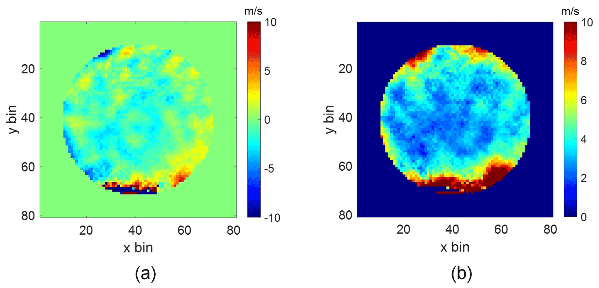
Figure 16 The difference between the expected and measured wind field is shown in panel (a) and the velocity standard deviation of the measured wind field across the field of view is shown in panel (b).

This standard deviation is slightly higher than that predicted using the Monte Carlo simulations. There are some possible error sources such as the impact of uncertainties in the calibrated instrument parameters, the stability of the laser, the residual errors of the thermal drift calibration and the presence of scattered laser light from the beam splitter. The analysis of these error sources was not performed for this study and will be undertaken in the future.

6 Discussion

The optical configuration of the breadboard prototype described in this paper has been used for lab testing, characterization and performance evaluation. Single-point wind measurements and two-dimensional wind measurements have been performed in the lab to examine the feasibility of the technique for the measurement of upper atmospheric winds. This work has also facilitated the identification of the primary practical issues that must be carefully considered to implement this instrument in the field. These include the following:

1. the sensitivity of the instrument to the field of view, misalignment of and mismatches in birefringent components,

2. the loss of quadrature across regions of the image which results in increased wind uncertainties within these regions,

3. thermal sensitivity of the field-widened birefringent interferometer and

4. availability of large-format high-quality Wollaston prisms and uniaxial birefringent slabs.

The impact of misalignments and mismatches was briefly discussed in Sect. 4. As shown in Fig. 8, as the field of view is increased, horizontal strips across the image are introduced that exhibit zero quadrature. Rotational misalignment between the lithium niobate slabs introduces hyperbolic fringes which changes the shape and increases the number and size of these zero-quadrature regions. Additionally, misalignment or manufacturing errors in the half-wave plate introduce parasitic fringes due to unequal coupling between the e and o waves in the interferometer. The overall impact of these sensitivities and the loss of quadrature between frames on the wind measurements must be investigated. This includes evaluating their effect on the accuracy of the calibrated fringe parameters, which also affect the precision of the wind measurements. A Jones matrix framework has been developed that allows these sensitivities to be examined by accurately simulating the interference fringes observed with the instrument (Langille et al., 2020). This framework was used in the design presented in Sect. 4 and provides a pragmatic and efficient means to evaluate and implement further refinements to the design and measurement approach.

In the case where the loss of quadrature within certain bands is present, we envision arranging a limb-viewing satellite instrument such that these bands are projected perpendicular to the horizon. In this case, there is only a loss of wind information over a small range horizontal bins at each tangent altitude. While these regions cannot provide wind information, they will provide simultaneous intensity profiles along the vertical dimension that can be combined to retrieve the vertical distribution of the volume emission rate.

The current BIDWIN configuration exhibits a strong thermal dependence that is dominated by the change in birefringence with temperature. This issue was managed for the lab measurements by using short integration times, sampling the non-rotating wheel between measurements and interpolating the thermal drift between measurements. This effect would need to be carefully managed in the case of a practical field instrument where longer integration times are required, by implementing thermal compensation and active thermal control. In this case, the thermal drift will be tracked (and then corrected) by observing a calibration source. This could be done periodically between scene measurements by observing a calibration source emitting a spectral line close to that of the target emission. Or it could be done simultaneously by observing a calibration source emitting a spectral line different from that of the target emission that is separated into a second channel by placing a dichroic filter in the exit optics. It may also be possible to partially thermally compensate the field-widened birefringent interferometer by combining appropriately selected and oriented slabs so that the temperature dependence of the two composite slabs is oppositely signed (Hale and Day, 1988). The design of the field calibration system and a thermally compensated field-widened birefringent interferometer requires careful and rigorous consideration that is outside the scope of the current work.

The final consideration relates to the availability of large-format high-quality Wollaston prisms and lithium niobate slabs. For the prototype design, the size of the Wollaston prisms rather than the field-widened birefringent delay plate limited the throughput, and as a result, it is much smaller than the maximum that is possible given the physical size of the delay plate. To realize the full capability of this design, a practical field instrument will need to utilize this larger throughput by acquiring custom large-format prisms. Given the availability of large-format crystals, a realistic field-widened birefringent interferometer can be constructed with effective path difference in the 0 to 2 cm range with diameters on the order of 100 mm. Therefore, instruments capable of achieving a throughput on the order of ∼1 cm² sr are feasible. Comparison of the effectiveness of a field-widened birefringent interferometer relative to a field-widened Michelson interferometer for the measurement of Doppler winds can be undertaken with respect to the primary instrument design parameters: A, Ω and D.

Table 6 Relative wind precision (E) evaluations for Michelson and birefringent interferometers (BIs). D: day, N: night.

For this comparison, we assume that both instruments are observing the same emission lines using the same integration time and that the wind precision is dominated by photon noise. By combining Eqs. (3) and (4), the wind uncertainty as a function of the source characteristics and the instrumental parameters is

$$\begin{array}{}\text{(16)}& {\mathit{\sigma }}_{\mathrm{w}}={\displaystyle \frac{c\mathit{\lambda }}{\mathrm{2}\sqrt{\mathrm{2}}\mathit{\pi }UVD\sqrt{\frac{{\mathrm{10}}^{\mathrm{6}}}{\mathrm{4}\mathit{\pi }}{I}_{\mathrm{0}}t\mathit{\eta }A\mathrm{\Omega }{\mathit{\tau }}_c}}}.\end{array}$$

The comparison is further simplified by assuming the instrumental parameters t, I₀, η and U are the same. Since the visibility, $V=e^{-{\mathrm{QTD}}^{\mathrm{2}}}$, is a function of D and T, it must also be included in the comparison. The instruments' relative wind-measuring precision, E, evaluated with respect to throughput, path difference and the line visibility V, is

$$\begin{array}{}\text{(17)}& E={\displaystyle \frac{\mathit{\lambda }}{VD\sqrt{A\mathrm{\Omega }{\mathit{\tau }}_c}}}.\end{array}$$

In evaluating AΩ, the size of one field of view is used with the corresponding collecting area. Therefore, in the cases where four copies of the image are formed, such as for the instrument discussed in this paper, it is at the expense of the intensity level in each of the four copies. We account for this effect here by multiplying the transmission coefficient of those instrument by 0.25. Table 6 lists the values of E for several Michelson interferometers, both built and proposed, and for the birefringent interferometer discussed in this paper, for four representative airglow emissions. For the birefringent interferometer, we also make the conservative estimate that 25 % of the samples will exhibit zero quadrature and will be unusable for wind measurements. According to this analysis, the prototype LiNbO₃ birefringent interferometer has a wind measurement error that is comparable to but still larger than that of several current field-widened Michelson interferometers. Therefore, as shown in Sect. 4.2, the prototype instrument could only be used for single-point ground-based instruments where all samples in the image are averaged to increase the SNR.

However, a practical field instrument that is equally matched to the field-widened Michelson interferometer can be achieved by utilizing slightly larger and longer crystals to increase the path difference to D=1 cm and increase the usable aperture area by a factor of at least 4. It is possible because the diameter of a LiNbO₃ crystal can reach 100 mm. Substituting these optimized instrument parameters (D=1 cm, UV∼0.9) into Eq. (4), we find that an SNR > 480 is required to achieve a wind precision <5 m s⁻¹. In the case of ground-based measurements of the O¹D emission at 630 nm, and assuming that the field is sampled into a 10 × 10 image and that 25 % of the image exhibits zero quadrature (see Sect. 4.2), we substitute E_o∼100 R, τ∼0.1, η∼0.9, AΩ=0.86 cm² sr/100 into Eq. (3) and we find that an SNR > 480 can be achieved for each spatial sample in ∼50 s. For a limb-imaging instrument, where the signal levels are much higher (E_o∼30 kR), this SNR can be achieved with 100 × 100 spatial samples, in roughly 16.6 s. Therefore, a wind precision of <5 m s⁻¹ is feasible with the proposed field instrument using practicable spatial and temporal sampling. This high precision is a result of the large throughput provided by the large-format LiNbO₃ crystals. Utilizing the large throughput provided by the birefringent interferometer requires that the other optics surrounding the interferometer are designed to accommodate it. This aspect will be examined in future work.

7 Conclusions

This paper presented the concept, design and performance testing of a compact static birefringent interferometer called BIDWIN. The overall measurement principle, as well as the optical system and interferometer configuration were described. The design and implementation of the lab prototype were presented, and the instrument parameters were carefully characterized and calibrated. The expected wind precision and the limitation of the field of view has been analyzed and the performance of the design was evaluated. The feasibility of measuring upper atmospheric winds with a precision of 5 m s⁻¹ using BIDWIN was validated by performing single-point wind and two-dimensional wind field observation in the lab. The practical limitations associated with the design of a large-throughput BIDWIN instrument capable of field measurements was discussed. Further study is needed to take full advantage of the technique; specifically, the ability to accommodate large-aperture optical components and to implement thermal compensation. The overall performance of the prototype demonstrates the feasibility of the technique for the measurement of upper atmospheric winds.