Accuracy in starphotometry

Starphotometry, the night-time counterpart of sunphotometry, has not yet achieved the commonly sought observational error level of 1 %: a spectral optical depth (OD) error level of 0.01. In order to address this issue, we investigate a large variety of systematic (absolute) uncertainty sources. The bright-star catalogue of extraterrestrial references is noted as a major source of errors with an attendant recommendation that its accuracy, particularly its spectral photometric variability, be significantly improved. The small field of view (FOV) employed in starphotometry ensures that it, unlike sun- or moonphotometry, is only weakly dependent on the intrinsic and artificial OD reduction induced by scattering into the FOV by optically thin clouds. A FOV of 45 arcsec (arcseconds) was found to be the best trade-off for minimizing such forward-scattering errors concurrently with flux loss through vignetting. The importance of monitoring the sky background and using interpolation techniques to avoid spikes and to compensate for measurement delay was underscored. A set of 20 channels was identified to mitigate contamination errors associated with stellar and terrestrial atmospheric gas absorptions, as well as aurora and airglow emissions. We also note that observations made with starphotometers similar to our High Arctic instrument should be made at high angular elevations (i.e. at air masses less than 5). We noted the significant effects of snow crystal deposition on the starphotometer optics, how pseudo OD increases associated with this type of contamination could be detected, and how proactive techniques could be employed to avoid their occurrence in the first place. If all of these recommendations are followed, one may aspire to achieve component errors that are well below 0.01: in the process, one may attain a total 0.01 OD target error.

1 Introduction

The nocturnal monitoring of semi-transparent atmospheric features, such as particles (aerosols, optically thin clouds) or gases (O₃, H₂O), can be performed using attenuated starlight in order to derive a spectral optical depth (OD). The passive remote sensing method of stellar spectrophotometry (known as starphotometry by the atmospheric remote sensing community) was accordingly introduced in the early 1980s (Alekseeva, 1980; Roddier, 1981). Despite some technological progress, accurate stellar spectrophotometry remains a challenge (Deustua et al., 2013; Bohlin et al., 2014). Its evolution, with an emphasis on problems particular to starphotometry, can be followed in Roscoe et al. (1993), Leiterer et al. (1995, 1998), Herber et al. (2002), Pérez-Ramírez et al. (2008a, b), Baibakov et al. (2009, 2015), and Ivănescu (2015).

The accuracy of the optical depth (OD) retrieval remains critical for (second spectral order) particle feature extraction methods, which require sub-0.01 optical depth precision error, as shown in Fig. 4 of O'Neill et al. (2001). Such a precision error would necessitate sub-0.01 accuracy error: this corresponds to the WMO (2005) recommendation (i.e. $\mathrm{0.005}+\mathrm{0.01}/m$, applied to a high star at air mass m=2) and, as a notable example, to the satellite-based (over-ocean) aerosol optical depth (AOD) retrieval accuracy for climate energy budget analyses (Chylek et al., 2003). Other technical and data processing challenges remain inasmuch as this relatively rare type of instrument, with only a few operational starphotometers worldwide, is still evolving.

Sunphotometry and, to some extent, moonphotometry are much more mature technologies. The current starphotometers cannot yet, for example, parallel the automated robustness of the Cimel sunphotometers in the AErosol RObotic NETwork (AERONET; see Holben et al., 2001, for a discussion of the Cimel instrument and the AERONET network). One can aspire to benefit from the accomplishments of the solar methodology and improve its nocturnal counterpart. An early and comprehensive analysis of sunphotometer-related errors and an outline of its data processing procedures were detailed in Shaw (1976), with subsequent contributions by Forgan (1994), Dubovik et al. (2000), Mitchell and Forgan (2003), and Cachorro et al. (2004).

OD retrieval, typically in the near-ultraviolet (near-UV) to near-infrared (NIR) spectral range, is based on the Beer–Bouguer–Lambert law of atmospheric attenuation. The detailed heterochromatic (wide spectral band) attenuation law was investigated by King (1952), Rufener (1963, 1986), and Young and Irvine (1967). While employing wide spectral bands enhances the signal-to-noise ratio of faint stars, the attenuation law is substantially simplified in the monochromatic approximation. Depending on the acceptable error, the approximation is generally valid for spectral bandwidths narrower than 50 nm (see Golay, 1974, pp. 47–50). The narrow bands typical of sunphotometry are also employed in starphotometry; however, accuracy requirements generally limit the operational star set to the brightest stars (visual magnitudes less than 3).

Beyond the fact that stellar photometric observations are currently not accurate enough, the lack of information on certain types of errors is even more problematic. Our purpose is to overcome such issues and enhance the starphotometry reliability. A comprehensive initial analysis of stellar photometry errors was detailed in Young (1974). Strategies for retrieving accurate photometric observations under variable optical depth conditions were proposed by Rufener (1964, 1986) and Gutierrez-Moreno and Stock (1966)¹. Those fundamental astronomical studies remained largely unreferenced in atmospheric science literature. In the present study, we invoke and complement them in order to identify and characterize most sources of systematic uncertainty. We expect that, with the proper approach, optical depth accuracy within 0.01 is achievable. That target aside, the very act of approaching this value is worthwhile, as it will increase the level of trust and reliability in starphotometry. We seek to achieve such a goal by identifying ways to mitigate the most important errors, whether by virtue of instrumental and/or retrieval-algorithm improvement or by improved observational strategies.

This paper consists of instrumental descriptions and a comprehensive development of OD retrieval methods followed by a detailed discussion of the error sources associated with each key OD retrieval parameter. It concludes with recommendations for achieving the 0.01 OD error goal. Most of the errors that we describe are of a general nature, although some are specific to our particular spectrometer-based starphotometers (Ivănescu et al., 2014). Throughout the paper, we use τ to represent the total vertical (columnar) optical depth². We employ “OD” as a generic acronym for optical depth with a different prefix for different components³.

We only focus on accuracy aspects, leaving precision and calibration errors to be addressed in subsequent studies. We also avoid the non-linear complications associated with measurements in the water vapour absorption bands (in the neighbourhood of 940 nm): this subject has already been extensively described in the studies of Galkin and Arkharov (1981), Halthore et al. (1997), and Galkin et al. (2011, 2010).

2 Observation conditions

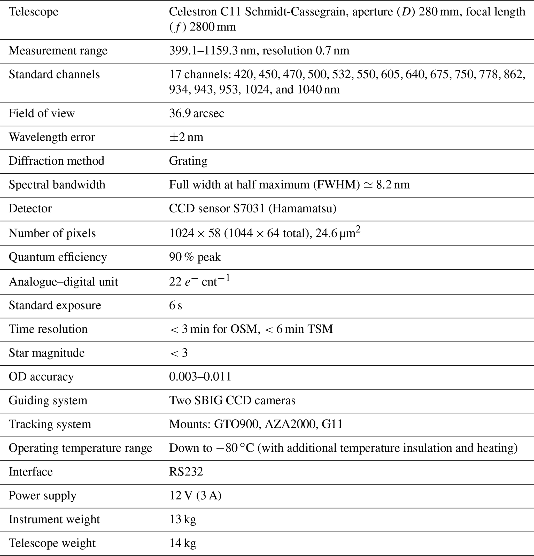
As detailed in Appendix A, the data reported in this paper were acquired using two similar instrument/telescope configurations that were designed and built by Dr. Schulz & Partner GmbH: the identical SPST05 and SPST06 instruments with an Intes Micro Alter M703 telescope, and the upgraded SPST09 instrument with a Celestron C11 telescope (all spectrometer-based photometers). In Appendix A, field of views (FOVs) of 57.3 and 36.9 arcsec were inferred for the earlier and upgraded instruments, respectively. SBIG CCD cameras were employed for star acquisition: their native camera pixels were binned into larger pixels of 3×3 native pixels, with an angular resolution of 3 arcsec per bin for the SPST05/M703 and 2 arcsec per bin for the SPST09/C11 instrument. Other technical parameters of the most recent version (SPST09/C11) are listed in Table 1.

Table 1 Technical parameters of the SPST09 starphotometer.​​​​​​​

The simultaneous measurement of all channels by all three spectrometer-based systems renders them particularly appropriate for observing rapidly evolving atmospheric features, such as optically thin clouds. This is important for purposes of coherent spectral analysis where all the channels have to capture the same sky view. Other starphotometer types are filter-wheel-based systems that sequentially observe one channel at a time (see, for example, Leiterer et al., 1995; Herber et al., 2002; Pérez-Ramírez et al., 2008b).

The observation sites included a variety of environments: warm, continental environment at the mid-latitude sites of Egbert and Sherbrooke; warm, continental and marine environment at the mid-latitude site of Halifax; warm and dry, tropical high-altitude site influenced by frequent Saharan dust events at Izaña; marine environment at the Low Arctic site of Barrow; and a cold and dry environment, influenced by the quasi-constant presence of ice crystals at the low-altitude, High Arctic site of Eureka. The latter is unique in terms of its extreme environmental conditions and the deployment of a larger telescope (C11). More details about the Eureka instrument and the observation facility (shown in Fig. 1), as well as its remote operation, are found in Ivănescu et al. (2014). One particular consideration of note in this case is the recurring frost formation on the telescope corrector plate and the quasi-constant deposition of ice crystals on it.

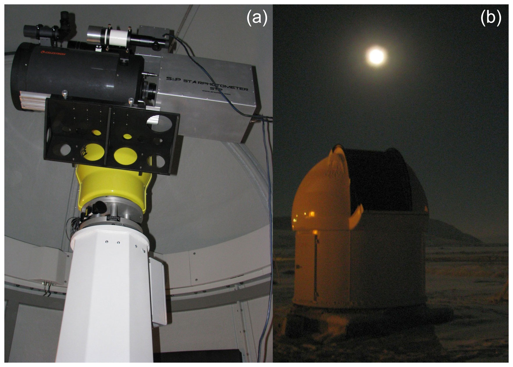
Figure 1 The SPST09 starphotometer and Celestron C11 telescope installed on the AZA-2000 mount, inside the Baader dome at Eureka (a). Outside view of the dome at Eureka, during a starphotometer observation (b).

Figure 2 shows observations, at Eureka and Sherbrooke, of starspot sizes (full width at half maximum (FWHM) ≡ω_s for short, quasi-instantaneous exposures and ω for long time exposures) as a function of the observed air mass. For the development of Fig. 2, we employed 5–40 short exposures per recording position. The (ω_s) exposure (integration) times were star dependent: they were varied from 1 to 30 s in order to avoid detector saturation for a given star. The exposure-to-exposure position change on the CCD of these short-exposure spots (the blue and black dots in Fig. 2) is largely influenced by turbulence jitter (Roddier, 1981). To account for this aspect and fully characterize the turbulence, one artificially creates long-exposure (1–4 min) spots by adding up the short-exposure spots on the CCD. The (ω) spot size of such a synthesized superposition of smaller spots will inevitably be relatively large and will be an average indicator of turbulence. We should note that the standard starphotometry integration times (6 s) are similar to those employed for Fig. 2 short exposure times: the reason that we create the long-duration spot size is to adequately characterize the low-frequency component of the turbulence. In this sense, an estimate of the true or total (all-frequency) turbulence requires the artificial generation of the long-exposure spots (a problem that is rather unique to bright-star starphotometry due to detector saturation concerns). Figures C1 and C2 show a schematic representation of a short-exposure starspot and two measured short-exposure starspot images acquired by the SBIG high-resolution camera (for two of the points in Fig. 2), respectively. Details on the theoretical and empirical context needed to understand the starspot computations is given in the associated text (Appendix C).

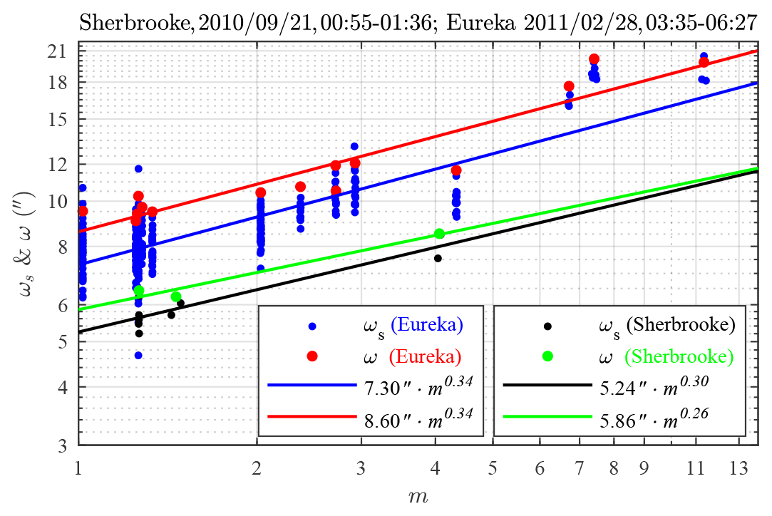
Figure 2 Very large starspots measured at the mid-latitude site of Sherbrooke, Québec, Canada (M703 telescope), and the High Arctic site of Eureka, Nunavut, Canada (C11 telescope), show a weaker air mass dependence than expected. The symbol ω_s is associated with short time exposures, whereas ω represents long time exposures. (Note that “′′” denotes arcseconds in this figure.)

In order to avoid any flux loss, the photometer FOV must be much larger than the FWHM of the short-exposure image, whose intensity profile (the star point spread function – PSF) can be approximated with a Gaussian profile (Racine, 1996). The total FWHM is then quadratically composed of the ω = FWHM of the “seeing” spot (the blurring due only to the air turbulence) and ω_d = FWHM of the Airy diffraction spot (approximated by a Gaussian profile whose FWHM is set equal to the FWHM of the diffraction spot). Optical aberrations due to incorrect collimation (especially coma for this type of telescope) may significantly affect the estimated seeing and the exponent of m. However, tests done at Airy Lab (AiryLab, 2012) show that the C11, when correctly collimated, is not subject to optical aberrations that influence the size of starspots as large as those in Fig. 2. The angular size of an Airy spot can be computed as ${\mathit{\omega }}_{\mathrm{d}}=\mathrm{1.03}\cdot \mathit{\lambda }/D$, where λ is the measurement wavelength. This gives less than 1 arcsec (0.49 arcsec for C11 and 0.75 arcsec for M703) at λ=640 nm (peak of CCD detection). As these values are 10–20 times smaller than the starspots, the observed FWHM is practically ω. Figure 2 indicates that, for typical atmospheric remote sensing sites (near sea level, not particularly dry, near heated buildings etc.), the expected seeing could be ∼10 times larger than what is usual in professional astronomy (∼1 arcsec). Uncontrolled telescope motion in strong winds may also increase the size of the recorded starspots. However, for the observational conditions associated with Fig. 2, the surface wind impact was negligible.

The turbulence strength can be assessed through the length parameter r₀ (Fried, 1966). If we assume negligible optical-aberration influences on the ω values in Fig. 2, the expression of Racine (1996) ($\mathit{\omega }=\mathrm{0.976}\cdot \mathit{\lambda }/r_{\mathrm{0}}$) yields r₀ values in the 5–15 mm range (about the size of the inner scale of turbulence). This means that the turbulence goes beyond the inertial Kolmogorov spectrum, normally producing starspot sizes dependent on m^0.6 (i.e. $m^{\mathrm{3}/\mathrm{5}}$) (Roddier, 1981), into the dissipation regime of the von Kármán spectrum (Osborn, 2010, pp. 16–17). This may explain the ∼0.3 exponent of m in Fig. 2: such a value corresponds to a von Kármán spectrum at high spatial frequencies (see, for example, Fig. 2.3 in Osborn, 2010). Also, as ω in Fig. 2 corresponds to an averaged λ=640, and as $\mathit{\omega }\sim {\mathit{\lambda }}^{-\mathrm{1}/\mathrm{5}}$, ω should be ∼10 % larger at 400 nm and ∼10 % smaller at 1000 nm.

With respect to the ω≃1 arcsec values usually experienced at high-altitude professional (non-amateur) astronomical sites, it is important to note the dramatically large values associated with the sea level (10 m altitude) Eureka station in Fig. 2. However, the seeing at the 610 m altitude Ridge Lab (CANDAC site, also at Eureka) is relatively very small (Steinbring et al., 2013) and is comparable with the best observation sites. One concludes that most of the turbulence at Eureka is confined in the first few hundred metres above sea level. It is instructive to characterize the vertical structure of the turbulence, notably its effect on the refractive index variation and, consequently, on star blurring (see, for example, Owens, 1967, for basics on the refractive index of air). Unfortunately, a precise characterization based solely on radiosonde measurements may not be possible (Roddier, 1981). However, that vertical structure can, nevertheless, be approximated parametrically. Accordingly, we express the vertical variation in the starspot size due to turbulence as

$$\begin{array}{}\text{(1)}& \mathrm{d}\mathit{\omega }=k_c\cdot k_t\cdot \mathrm{d}n\cdot \mathrm{d}v/v,\end{array}$$

where $\mathrm{d}v/v$ is the relative wind shear (whose kinetic turbulent energy is the primary influence on the refractive index variation, dn, between the atmospheric layers). This empirically derived equation provides a convenient (approximate) representation of ω versus altitude. The parameter k_t≃6 is a normalizing constant that adjusts the right side of Eq. (1) so that its integration yields the surface-level ω values in Fig. 2. Obviously, this constant may change if those values are plagued by significant optical aberrations. Employing an ensemble of Eureka, polar winter sounding profiles acquired over a ∼6-week period within the Fig. 2 measurement period, we integrated the dω² interpretation of those profiles from the maximum altitude of the radiosonde to a given altitude in order to yield ω at every altitude (Fig. 3). On the median (red) and average (green) curves one can identify major blurring increases: just below 3 km, below 200–400 m (suggesting a quasi-permanent turbulent layer), and again about 10–20 m from the surface. This confirms the very low ω values at the Ridge Lab, despite the dramatically large seeing at sea level.

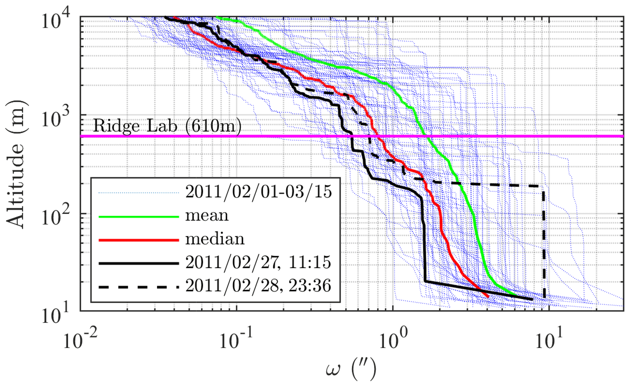
Figure 3 Vertical structure of starspot blurring at Eureka derived from the quadrature integration of Eq. (1). Most of the turbulence is below the Ridge Lab elevation (magenta line). The black curves were derived from the two nearest soundings to the ω measurements in Fig. 2. The k_t=6 (derived for the black curves) was employed for all the other curves. (Note that “′′” denotes arcseconds in this figure.)

3 Observation methodology

A photometric system, from the perspective of the astronomical community, is a system assessing the brightness of an object on a logarithmic scale, normalized to a standard reference (a natural source or a convenient synthetic spectrum).

3.1 Catalogue photometric system

We use I to denote the star irradiance expressed in absolute measurement units. By definition, the apparent magnitude (M) of a star is computed from the ratio between I (the observed irradiance) and I_0,cref, the unattenuated (“0”) irradiance of a “catalogue reference” (“cref”) source:

$$\begin{array}{}\text{(2)}& M=-\mathrm{2.5}\log {\displaystyle \frac{I}{I_{\mathrm{0},\text{cref}}}}=-\mathrm{2.5}\log I+\mathrm{2.5}\log I_{\mathrm{0},\text{cref}},\end{array}$$

where “log” is short for “log ₁₀”. The quantity

$$\begin{array}{}\text{(3)}& \text{ZP}=\mathrm{2.5}\log I_{\mathrm{0},\text{cref}}\end{array}$$

is usually referred to as the “zero-point” of the photometric system and serves, from a practical standpoint, to identify the photometric system. Star magnitudes are, therefore, photometric-system dependent. The magnitude of the reference source at any wavelength is, by definition, $M_{\mathrm{0},\text{cref}}=\mathrm{0}$ (i.e. when $I=I_{\mathrm{0},\text{cref}}$). Most of the photometric systems currently employed are based on Vega as a primary reference source (“primary standard”) (Bessell, 2005).

One can recast Eq. (2) into its “extraterrestrial” form

$$\begin{array}{}\text{(4)}& M_{\mathrm{0}}=-\mathrm{2.5}\log {\displaystyle \frac{I_{\mathrm{0}}}{I_{\mathrm{0},\text{cref}}}}=-\mathrm{2.5}\log I_{\mathrm{0}}+\mathrm{2.5}\log I_{\mathrm{0},\text{cref}}.\end{array}$$

The adjective extraterrestrial can also be represented by “unattenuated”, “extra-atmospheric”, “exoatmospheric”, or “zero air mass” in the literature (ground-based measurements are also referred to as “attenuated”). The signature extraterrestrial magnitudes of each star are found in the catalogue(s) of various observation campaigns. M₀, obtained with the V standard wideband filter (Johnson and Morgan, 1953), covering most of the visible spectrum, is usually called visual V magnitude. The blue B magnitude is then obtained with their B-band filter, etc.

The most accurate exoatmospheric star irradiance catalogue in the starphotometry spectral range is that from Pulkovo (Alekseeva et al., 1996). This catalogue provides near-UV to NIR I₀ spectra⁴ for most of the brightest stars (V<3). Its magnitudes (Alekseeva et al., 1994) are simply expressed as

$$\begin{array}{}\text{(5)}& M_{\mathrm{0}}=-\mathrm{2.5}\log I_{\mathrm{0}},\end{array}$$

with I₀ converted to cgs units of $\mathrm{erg}{\mathrm{s}}^{-\mathrm{1}}{\mathrm{cm}}^{-\mathrm{2}}{\mathrm{cm}}^{-\mathrm{1}}$. From Eqs. (3) and (4), one concludes that ZP = 0 in Eq. (5). Therefore, the reference spectrum used to compute the Pulkovo catalogue magnitudes is spectrally flat and equal to unity ($I_{\mathrm{0},\text{cref}}=\mathrm{1}$ $\mathrm{erg}{\mathrm{s}}^{-\mathrm{1}}{\mathrm{cm}}^{-\mathrm{2}}{\mathrm{cm}}^{-\mathrm{1}}$). Such a unit reference defines a “raw” photometric system (or “raw” magnitudes). Its SI-unit value of 0.1 $\mathrm{W}{\mathrm{m}}^{-\mathrm{2}}{\mathrm{m}}^{-\mathrm{1}}$ is near the Vega irradiance maximum of 0.0796 $\mathrm{W}{\mathrm{m}}^{-\mathrm{2}}{\mathrm{m}}^{-\mathrm{1}}$ at 402.5 nm (when measured at a 8.2 nm bandwidth)⁵.

3.2 Theoretical considerations

The starphotometer measurement principle is based on the Beer–Bouguer–Lambert attenuation law applied to the starlight passing through the Earth's atmosphere (as described, for example, in Liou, 2002). The attenuation, due to the out-scattering and absorption of the incoming light by atmospheric particles and gases, is described by

$$\begin{array}{}\text{(6)}& I=I_{\mathrm{0}}{e}^{-m\mathit{\tau }},\end{array}$$

where τ is the total vertical optical depth, m is the stellar air mass, and I and I₀ are the attenuated and unattenuated star irradiances, respectively. For a plane-parallel atmosphere approximation, $m=\mathrm{1}/\cos \mathit{\theta }$, where θ is the zenith angle of a given star (the approximation is generally valid for θ≲80^∘, or m≲6).

The law formulated in Eq. (6) can be more practically converted into a linear form by expressing it in term of apparent magnitudes, M and M₀, as defined in Eqs. (2) and (4), respectively. Taking the logarithm of Eq. (6), one obtains

$$\begin{array}{}\text{(7)}& \log {\displaystyle \frac{I}{I_{\mathrm{0}}}}=-{\displaystyle \frac{M-M_{\mathrm{0}}}{\mathrm{2.5}}}=-m\mathit{\tau }\log e,\end{array}$$

where e is the natural logarithm base. The exponential law then becomes a linear relation in terms of apparent magnitudes:

$$\begin{array}{}\text{(8)}& M=M_{\mathrm{0}}+\mathrm{2.5}\log e\cdot m\mathit{\tau }=M_{\mathrm{0}}+(m/\mathrm{0.921})\mathit{\tau }.\end{array}$$

This expression, under conditions of approximately constant τ, can be used to retrieve the intercept M₀ from a linear regression of M versus m. This can be done, for example, by employing a series of irradiance measurements carried out over a clear night with significant changes in m (not always a given in the case of a High Arctic site). Such a procedure is referred to as the Langley calibration technique, or Langley plot (also described in Liou, 2002).

3.3 Practical considerations

The measured star signal (F) is expressed in counts per second (cnt s⁻¹). If F_0,iref is the unattenuated “instrument reference” signal, defining the instrument photometric system (in cnt s⁻¹), the attenuated and unattenuated instrumental magnitudes (S and S₀, respectively) can be expressed, in a manner analogous to Eqs. (2) and (4), respectively:

$$\begin{array}{}\text{(9)}& S=-\mathrm{2.5}\log {\displaystyle \frac{F}{F_{\mathrm{0},\text{iref}}}};S_{\mathrm{0}}=-\mathrm{2.5}\log {\displaystyle \frac{F_{\mathrm{0}}}{F_{\mathrm{0},\text{iref}}}}.\end{array}$$

One can convert F into I with an instrument-specific conversion factor:

$$\begin{array}{}\text{(10)}& c={\displaystyle \frac{I}{F}}.\end{array}$$

Applied to the two system references, the ratio becomes

$$\begin{array}{}\text{(11)}& c_{\text{ref}}={\displaystyle \frac{I_{\mathrm{0},\text{cref}}}{F_{\mathrm{0},\text{iref}}}}.\end{array}$$

This represents a transformation (scaling) factor from the instrument to the catalogue reference system. The unitless $c/c_{\text{ref}}$ ratio then incorporates the photometric-system scaling (c_ref) as well as the optical and electronic throughput of the instrument (c). In terms of magnitudes, we can define the instrument-specific calibration parameter as

$$\begin{array}{}\text{(12)}& C=-\mathrm{2.5}\log {\displaystyle \frac{c}{c_{\text{ref}}}}=-\mathrm{2.5}\log {\displaystyle \frac{I}{I_{\mathrm{0},\text{cref}}}}+\mathrm{2.5}\log {\displaystyle \frac{F}{F_{\mathrm{0},\text{iref}}}}.\end{array}$$

Substituting S and S₀ from Eq. (9) as well as M and M₀ from Eqs. (2) and (4) into Eq. (12) yields

$$\begin{array}{}\text{(13)}& {\displaystyle }C=M-S\end{array}$$

and

$$\begin{array}{}\text{(14)}& {\displaystyle }C=M_{\mathrm{0}}-S_{\mathrm{0}},\end{array}$$

where the role of C as a conversion factor between the catalogue and instrument magnitudes is made readily apparent by the elegant simplicity of this pair of equations.

If the catalogue reference is the unattenuated source being observed, I₀ = I_0,cref and $M_{\mathrm{0},\text{cref}}=\mathrm{0}$, as per Eq. (4). Accordingly, from Eq. (14), $C=-S_{\mathrm{0},\text{cref}}$. Alternatively, if the instrumental reference is the unattenuated source being observed, $F_{\mathrm{0}}=F_{\mathrm{0},\text{iref}}$ and $S_{\mathrm{0},\text{iref}}=\mathrm{0}$, as per Eq. (9). Equation (14) then indicates that $C=M_{\mathrm{0},\text{iref}}$ (i.e. the catalogue magnitude of the instrument reference source). Equating the C values for those two special cases yields $M_{\mathrm{0},\text{iref}}=-S_{\mathrm{0},\text{cref}}$. In addition, the calibration parameter may be expressed as

$$\begin{array}{}\text{(15)}& C=-S_{\mathrm{0},\text{cref}}=\mathrm{2.5}\log F_{\mathrm{0},\text{cref}}=\ln F_{\mathrm{0},\text{cref}}/\mathrm{0.921},\end{array}$$

where F_0,cref is the instrument signal measured when observing the star catalogue reference.

In practice, Eq. (9) is often expressed as

$$\begin{array}{}\text{(16)}& S=-\mathrm{2.5}\log F=-\ln F/\mathrm{0.921}\end{array}$$

and

$$\begin{array}{}\text{(17)}& S_{\mathrm{0}}=-\mathrm{2.5}\log F_{\mathrm{0}}=-\ln F_{\mathrm{0}}/\mathrm{0.921}.\end{array}$$

This either implies that F and F₀ are unitless (i.e. measurements are already normalized to the instrument reference) or that the reference is conveniently chosen as $F_{\mathrm{0},\text{iref}}=\mathrm{1}$ cnt s⁻¹ (ZP = 0). Such a unit reference, as in the case of the catalogue system, defines a “raw” photometric system (as is employed for our starphotometers). According to Eq. (11), having unit values for both photometric system references implies that the scaling factor is also unity (c_cref=1). This yields

$$\begin{array}{}\text{(18)}& C=-\mathrm{2.5}\log c=-\mathrm{2.5}\log {\displaystyle \frac{I}{F}}=-\mathrm{2.5}\log {\displaystyle \frac{I_{\mathrm{0}}}{F_{\mathrm{0}}}}.\end{array}$$

The calibration procedure then reduces to the unattenuated measurement of any source of known irradiance. Equation (18) may be used in laboratory-based calibrations or in “in situ” calibrations by measuring any accurately known star spectra. This may be done in a Rayleigh atmosphere (i.e. without aerosol or clouds), for which the attenuation can be accurately estimated (Bucholtz, 1995). Such conditions can generally be approximated at high-elevation calibration sites (supported by some independent estimate of the small but non-negligible aerosol optical depth).

If we define, for simplicity,

$$\begin{array}{}\text{(19)}& x=m/\mathrm{0.921},\end{array}$$

Eq. (8) can be rewritten as

$$\begin{array}{}\text{(20)}& M=\mathit{\tau }x+M_{\mathrm{0}}.\end{array}$$

Substituting M from Eq. (13) into Eq. (20) yields a Langley calibration equation whose ground-based (τ-dependent) component is expressed in terms of the instrument signal S:

$$\begin{array}{}\text{(21)}& M_{\mathrm{0}}-S=-\mathit{\tau }x+C.\end{array}$$

This expression enables the retrieval of C when M₀ is provided by a catalogue. However, if an accurate M₀ spectrum cannot be found, Eq. (14) can be used to transform Eq. (21) into a pure instrumentation version

$$\begin{array}{}\text{(22)}& S=\mathit{\tau }x+S_{\mathrm{0}}\end{array}$$

so that a catalogue is no longer required. Instead of finding C, one has to employ Langley calibrations to estimate S₀ for all stars that are part of the operational protocol of a given starphotometer. Equation (21), in contrast, has the advantage of casting the calibration procedure in terms of an explicit function of a single star-independent constant (C). C represents an intrinsic parameter that remains constant as long as the instrument characteristics do not change.

3.4 Measuring methods

The main purpose of starphotometer measurements is to provide an estimate of the optical depth (τ). The Langley calibration enabled by Eq. (21) allows the direct retrieval of τ as the slope of a linear regression between S and x. This is typically a lengthy procedure (hours) involving several single-star measurements over large x variations and an assumption of negligible OD variation.

3.4.1 One-star method (OSM)

Retrieval of τ values for every S sample can, nevertheless, be achieved with a pre-calibrated instrument. In terms of the OSM, Eqs. (21) and (22) can be rearranged to yield

$$\begin{array}{}\text{(23)}& \mathit{\tau }={\displaystyle \frac{S-S_{\mathrm{0}}}{x}}={\displaystyle \frac{S-M_{\mathrm{0}}+C}{x}}.\end{array}$$

This approach is particularly useful in the presence of rapid τ variations that one observes, for example, during cloud events. As the OSM requires constant and accurately predetermined calibration values, any optical or electronic degradation of the instrument will propagate into the τ estimation.

Δ OSM

An OD retrieval that does not require calibration (or any extra-atmospheric instrumental reference) may be achieved using finite differences applied to Eq. (22) (for two measurements of the same star, acquired at times A and B):

$$\begin{array}{}\text{(24)}& \mathit{\tau }={\displaystyle \frac{S_A-S_B}{x_A-x_B}}={\displaystyle \frac{\mathrm{\Delta }S}{\mathrm{\Delta }x}}.\end{array}$$

S_A and S_B have to be acquired in the presence of negligible τ variation over sufficiently large Δx in order to reduce the impact of measurement errors. The Δx constraint may be impossible or, at best, represents hours of time for stars in the High Arctic. It is more readily achieved at low-latitude sites, but it is generally too slow to capture anything but very low-frequency OD variability.

3.4.2 Two-star method (TSM)

Accurate τ retrieval over a short period of time (minutes) may also be achieved with an uncalibrated instrument by near-synchronous observation of two stars at significantly different air mass⁶. This procedure, known as TSM (two-star method) englobes the Δ TSM and ΔΔ TSM variants described below.

Δ TSM

The Δ TSM variant⁷ is obtained using finite differences applied to Eq. (21) for stars “1” and “2”, corresponding to a low (or large air mass) star and to a high (or small air mass) star, respectively:

$$\begin{array}{}\text{(25)}& \mathit{\tau }={\displaystyle \frac{(S_{\mathrm{1}}-S_{\mathrm{2}})-(M_{\mathrm{0},\mathrm{1}}-M_{\mathrm{0},\mathrm{2}})}{x_{\mathrm{1}}-x_{\mathrm{2}}}}={\displaystyle \frac{\mathrm{\Delta }S-\mathrm{\Delta }{M}_{\mathrm{0}}}{\mathrm{\Delta }x}}.\end{array}$$

The TSM requirement of a large air mass difference minimizes OD errors associated with the TSM variants. The impact of larger measurement errors beyond air mass 5 may, however, attenuate the benefits of a large air mass range (see Young, 1974, for an optimization analysis). In practice, the x range of the high-star is 1–2, whereas the low-star range is 3–5. The “auto-calibrating” feature of Eq. (25) (i.e. no need for C or S₀) is limited in its applicability: the temporal and spatial variation in τ between the two observations must be small: this limits the method to the types of homogeneous sky transparency conditions associated with the presence of background aerosols or thin homogeneous clouds. The larger low-star air mass requirement can also incite throughput variation induced by air-mass-dependent starlight-vignetting variations (see Sect. 7.1).

This TSM variant can be interpreted as a two-star Langley for which C is determined by a “regression” through only two data points:

$$\begin{array}{}\text{(26)}& C={\displaystyle \frac{(M_{\mathrm{0},\mathrm{2}}-S_{\mathrm{2}})/x_{\mathrm{2}}-(M_{\mathrm{0},\mathrm{1}}-S_{\mathrm{1}})/x_{\mathrm{1}}}{\mathrm{1}/x_{\mathrm{2}}-\mathrm{1}/x_{\mathrm{1}}}}.\end{array}$$

This amounts to the insertion of τ from Eq. (25) into Eq. (21). Employing the same τ for both stars in Eq. (21) will also provide two calibration instances, C₁ and C₂. Combining Eqs. (26) and (21) yields a weighted C average of the form

$$\begin{array}{}\text{(27)}& C={\displaystyle \frac{C_{\mathrm{2}}/x_{\mathrm{2}}-C_{\mathrm{1}}/x_{\mathrm{1}}}{\mathrm{1}/x_{\mathrm{2}}-\mathrm{1}/x_{\mathrm{1}}}},\end{array}$$

where the weights are signed values of $\mathrm{1}/x$. Such a C value obtained from two data points will clearly be less accurate than that obtained from a calibration using numerous measurement points (as used in OSM Eq. 23). Thus, the Δ TSM variant is only employed when more accurate calibration schemes are not available. Even if τ should operationally be computed with the OSM, it is advantageous to employ the Δ TSM variant to pinpoint the occurrence of throughput degradation events. This is critical at low-altitude operational observatories that are prone to dust, dew, frost, or snow deposition on the telescope optics (see Sect. 7.6).

If, in contrast, the instrument throughput is known to be stable, the acquisition of a large set of Δ TSM measurements may enable an accurate calibration under variable τ conditions. Several TSM-based procedures optimizing S₀ retrieval are detailed in Stock (1969) and Mironov (2008), while an iterative algorithm, employed at the Pulkovo observatory, is detailed in Novikov (2021). Such retrievals of sets of S₀ are equivalent to building a new M₀ catalogue. For example, the average of Eq. (14) may be used over a large number of stars to obtain $M_{\mathrm{0}}\cong S_{\mathrm{0}}+\stackrel{\mathrm{‾}}{C}$. This task is, however, expected to produce better results at a high-altitude calibration observatory. Conversely, averaging Eq. (26), with accurately predetermined M₀ values, opens up the prospect of a star-independent calibration, even at a low-altitude site under variable τ conditions.

ΔΔ TSM

Gutierrez-Moreno and Stock (1966) introduced the ΔΔ TSM variant to reduce Δ TSM error propagation associated with errors in M₀ (see Stock, 1969, for further ΔΔ TSM details and Sect. 4 for a discussion of M₀ errors). This variant is obtained by using double (two-star) finite differences applied to Eq. (21),

$$\begin{array}{}\text{(28)}& \mathit{\tau }={\displaystyle \frac{(S_{\mathrm{1},A}-S_{\mathrm{2},A})-(S_{\mathrm{1},B}-S_{\mathrm{2},B})}{(x_{\mathrm{1},A}-x_{\mathrm{2},A})-(x_{\mathrm{1},B}-x_{\mathrm{2},B})}}={\displaystyle \frac{\mathrm{\Delta }\mathrm{\Delta }S}{\mathrm{\Delta }\mathrm{\Delta }x}},\end{array}$$

acquired near the nominal times of A and B, separated by hours, as in the case of Δ OSM. This method is also too slow to capture anything but very low-frequency OD variability. Usually, one seeks to maximize ΔΔx in order to minimize S error propagation: the standard scenario is that the stars exchange their positions near the meridian (a star dynamic that is only feasible at low latitudes).

3.5 Optical depth accuracy

In reality, we cannot measure the starlight alone, as the measurement always includes a background signal B. The latter is mainly due to the electronic readout signal and sky brightness. If R is the starphotometer measurement obtained while pointing towards the star, then B can be estimated by a slightly off-axis measurement. In dark-sky conditions, B is dominated by the instrument dark current. The desired starphotometer (starlight) signal is estimated as

$$\begin{array}{}\text{(29)}& F=R-B,\end{array}$$

with attendant systematic error components

$$\begin{array}{}\text{(30)}& {\mathit{\delta }}_F={\mathit{\delta }}_R+{\mathit{\delta }}_B.\end{array}$$

For small relative errors ${\mathit{\delta }}_F/F$, one obtains δ_S by taking the derivative $\left|S^{\prime }\right|$ of S with respect to F in Eq. (16):

$$\begin{array}{}\text{(31)}& {\mathit{\delta }}_S=\left|S^{\prime }\right|{\mathit{\delta }}_F=\mathrm{1.0857}{\displaystyle \frac{{\mathit{\delta }}_F}{F}}.\end{array}$$

If the only errors are in S, Eq. (23) yields

$$\begin{array}{}\text{(32)}& {\mathit{\delta }}_{\mathit{\tau }}={\displaystyle \frac{{\mathit{\delta }}_S}{x}}={\displaystyle \frac{\mathrm{1}}{m}}{\displaystyle \frac{{\mathit{\delta }}_F}{F}}.\end{array}$$

However, the optical depth accuracy is subject not only to errors in the observational parameter (S) but also to all of the other physical parameters (M₀, C, x) involved in the starphotometry retrieval. All of the contributions to the line-of-site observation error can be explicitly listed by differentiating Eq. (23):

$$\begin{array}{}\text{(33)}& {\mathit{\delta }}_{\mathit{ϵ}}\equiv x{\mathit{\delta }}_{\mathit{\tau }}=-{\mathit{\delta }}_{M_{\mathrm{0}}}-{\mathit{\delta }}_x\mathit{\tau }+{\mathit{\delta }}_S+{\mathit{\delta }}_C.\end{array}$$

The other components of the observation error that represent magnitudes (M₀ and C, as per Eqs. 5 and 18, respectively) can, in a similar fashion to Eq. (31), be expressed as follows:

$$\begin{array}{}\text{(34)}& {\mathit{\delta }}_{M_{\mathrm{0}}}=\mathrm{1.0857}{\displaystyle \frac{{\mathit{\delta }}_{I_{\mathrm{0}}}}{I_{\mathrm{0}}}};{\mathit{\delta }}_C=\mathrm{1.0857}{\displaystyle \frac{{\mathit{\delta }}_{\mathrm{c}}}{c}}.\end{array}$$

A comprehensive description of starphotometry-related errors can be found in Young (1974) and Carlund et al. (2003). In the following sections we continue this work by quantifying the accuracy of each individual parameter of Eq. (33) (M₀, x, S, and C).

4 Spectrophotometric catalogue (M₀) accuracy

In order to move from a star-dependent S₀ calibration, which is currently the standard (Rufener, 1986; Pérez-Ramírez et al., 2011), to the more convenient star-independent calibration in terms of C, one has to ensure that the exoatmospheric magnitudes M₀ are sufficiently accurate.

4.1 Pulkovo catalogue errors

The star dataset that we employed (Appendix B) was limited to stars with a maximum of 0.01 magnitude variation in the observations used to generate their Pulkovo catalogue entry (that dataset was employed as the default catalogue by the manufacturer of our instruments). They are mostly main-sequence stars (of luminosity class V) (Kippenhahn et al., 2012) at the most stable period of their life cycle (five are of luminosity class II–III). Five are “early-type” spectral-class-B stars (i.e. B0–B3), one is a “late-type” class-A star (i.e. A7–A9), and one is a class-F star. They are all characterized by weaker absorption lines and cleaner continuum (Silva and Cornell, 1992). However, the “early-type” B stars may also experience non-negligible (0.01-magnitude) photometric variability (Eyer and Grenon, 1997). Beyond their intrinsic photometric stability, the M₀ accuracy remains a concern. Alekseeva et al. (1996) stated that “to preserve the uniform absolute system for all our seasonal catalogues, we always used the same energy distribution of Vega based on the absolute calibrations by Oke and Schild (1970) and Kharitonov et al. (1978)”. In other words, Vega data were calibrated to the accuracy level achievable about 50 years ago. In addition, Knyazeva and Kharitonov (1990) specified that their (Kharitonov et al., 1978) calibration values were actually subject to systematic errors that could be as large as 10 %. In spite of the shortcomings of the Pulkovo catalogue, it remains the most accurate catalogue in terms of representing the entire bright-star dataset of Appendix B. By comparison, the Hubble Space Telescope (HST) dataset includes only a few of those stars. To better understand the impact of the Pulkovo catalogue shortcomings, we compared its absolute irradiances with those measured by the HST. This higher-accuracy dataset only contains a few bright stars: Vega (HR7001) and Sirius (HR2491) from the CALSPEC Calibration database (Bohlin et al., 2014), and HR15, HR2618, and HR4295 from the Hubble Space Telescope Imaging Spectrograph (STIS) New Generation Stellar Library (NGSL) (Bohlin et al., 2001). As HST measurements are performed with a more recent technology, are not subject to atmospheric effects, and have absolute errors below 1 % (Bohlin, 2014), we considered them to be the reference. The corresponding magnitude differences between the Pulkovo and HST spectra, computed in terms of the Pulkovo photometric system, are presented in Fig. 4. Within a context of the potential impact of atmospheric errors, it is remarkable that more than half of the standard starphotometer channels (open circles) are characterized by errors of less than 2 % or equivalently δM₀<0.02 (Eq. 34) for a catalogue derived from ground-based measurements. Based on the average difference in Fig. 4, one nevertheless concludes that the Pulkovo catalogue is characterized by a bias that is particularly large in the near-UV and in the 900–1000 nm range. These biases may, in part, be attributable to uncertainties related to the stronger aerosol scattering effects in the UV and to water vapour effects in the NIR region. The average bias found in Fig. 4 could then be used to correct the Pulkovo catalogue. However, a bias will not actually affect the optical depth measurements. For example, in the Δ TSM mode, such a bias is cancelled out in the M₀ magnitude difference of Eq. (25). Even in the OSM mode of Eq. (23), the bias will actually propagate into C during the calibration process. This bias transfer is attributable to the fact that a bias will only affect the intercept of the Langley plot, not its slope, as expressed by Eq. (21). The δM₀ standard deviation in Fig. 4 (∼0.02), can, on its own merits, be compared with the accuracy of 0.015–0.02 claimed for the Pulkovo catalogue (Alekseeva et al., 1996), although these values increase in the UV and water vapour channels. One should also note that for its primary reference stars, such as Vega and Sirius, the 0.02 Pulkovo catalogue upper limit of error is halved. Such error levels will impact information extraction from optical depth spectra, especially as the required accuracy for aerosol retrievals sensitive to higher orders of the AOD spectrum is ∼0.01 (O'Neill et al., 2001).

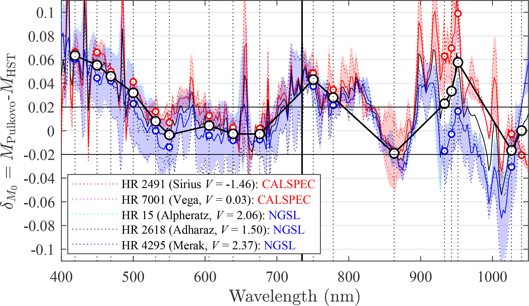
Figure 4 Spectrophotometric bias (δM₀) of the Pulkovo catalogue with respect to two different HST catalogues (CALSPEC and NGSL). Open circles represent our standard starphotometer channels, solid coloured lines are δM₀ averages for each HST catalogue, and the coloured shading represents the corresponding standard deviations. For each spectrum point, the two coloured curves and their shading represent sampling populations of two points (stars) for the red CALSPEC catalogue and three points (stars) for the blue NGSL catalogue: our objective here was to obtain an estimate of δM₀ statistics assuming δM₀ values were roughly independent of the M₀ values of individual stars.

4.2 Bandwidth mismatch error

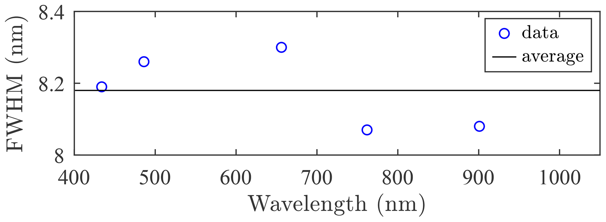
Figure 5 shows the quasi-constant 8.2 nm bandwidth measured by observing Vega with the SPST09/C11 system. Those FWHM estimates are line-broadening measures of the strong hydrogen (H) Balmer series (H_α=656.3 nm, H_β=486.1 nm, and H_γ=434.1 nm, but not H_δ=410.2 nm). These are absorption lines in the star's own atmosphere and are accordingly intrinsic to the exoatmospheric stellar spectra. We also employed the telluric (i.e. Earth's atmosphere) O₂ line at 762 nm and another NIR line specific to Vega. The observations used for the Pulkovo catalogue were, in contrast, made at a 5 nm bandwidth over the 310–735 nm range and at 10 nm over the 735–1105 nm range (at a 2.5 nm nominal resolution). For bandwidth consistency over the entire 310–1105 nm range, Alekseeva et al. (1996) reprocessed the 5 nm measurements to synthesize a unique 10 nm bandwidth. Currently, we only use the 10 nm bandwidth version over the entire 310–1105 nm range. However, as noted in Young (1992), a bandwidth mismatch between the catalogue and the instrument (i.e. 10 and 8.2 nm in our case, respectively) may have an impact on the optical depth error and merits investigation. In order to assess the impact of the bandwidth mismatch, we compared the magnitude errors when using M_5.0 and M₁₀, associated with the 5 and 10 nm bandwidths, instead of the actual magnitude M_8.2 at a 8.2 nm bandwidth. We also assessed how a simple magnitude calculation $(M_{\mathrm{5.0}}+\mathrm{2}{M}_{\mathrm{10}})/\mathrm{3}$ compares with the actual 8.2 nm bandwidth, in order to improve the actual 10 nm bandwidth catalogue. We synthesized star magnitudes for those three different bandwidths by applying Gaussian bandpass filters to the HST data (originally at a 1 Å resolution). This is, in fact, a convolution operation that effectively blurs the stellar absorption lines.

Figure 5 SPST09/C11 bandwidth measured with Vega.

In Fig. 6, we compare the magnitudes computed for the three bandwidths, for a star of spectral class A0 (Vega). Figure 6a shows a spectral zoom about the 420 nm starphotometer channel. The increased broadening with increasing FWHM about the H_γ and H_δ Balmer lines demonstrates the blurring effect of the different bandwidths. The graph also shows that one may actually limit the blurring impact by optimizing the spectral location of a given channel. Moving the 420 nm channel to 423 nm will, for example, significantly reduce that impact. Figure 6b shows the contamination due to different blurring levels for the entire spectrum (contamination expressed in terms of δM₀, which from Eq. 33 is, in the absence of other errors, equivalent to xδ_τ. The spiky, high-frequency nature of the δM₀ spectra demonstrates that, while most of the starphotometer channels have negligible (<0.01) errors, channels in the blue and the NIR are significantly affected. The black curve “$\mathit{\delta }{M}_{\mathrm{0}}=M_{\mathrm{8.2}}-(M_{\mathrm{5.0}}+\mathrm{2}{M}_{\mathrm{10}})/\mathrm{3}$” demonstrates that one may approximate a spectral convolution using a simple average of twice the upper and once the lower bound magnitudes.

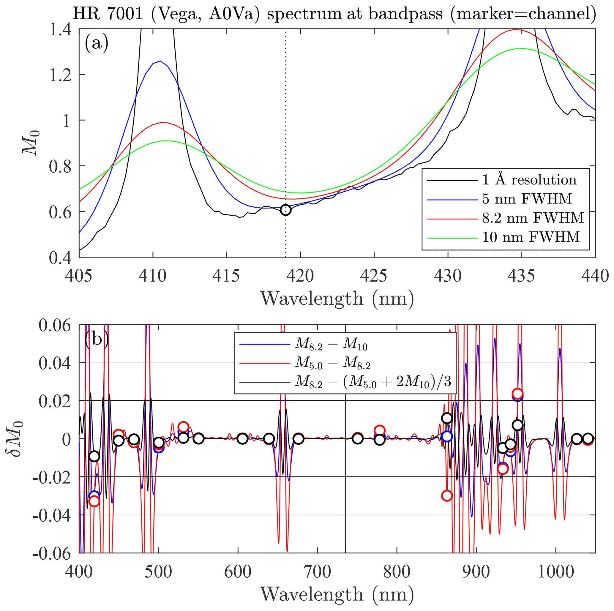
Figure 6 Bandwidth mismatch error for a star of spectral class A (Vega, HR7001). Open circles are the nominal starphotometer channels.

The same exercise carried out for a star of early-type spectral class B (Adharaz) underscores the fact that the H Balmer lines are much weaker (Fig. 7a). One expects similar behaviour for our “late-type” A- and F-class stars. Consequently, the blurring contamination over the entire spectrum (Fig. 7b) is, for the case that concerns us the most (M_8.2−M₁₀), largely less than 0.01, except for the 958 nm channel that is too close to the 954.6 nm H Paschen absorption line. Inasmuch as all of our operational stars are of class A and B (except for one F-class star), this analysis is representative. As the bandwidth mismatch error is a bias that differs for the two respective star classes shown in Figs. 6 and 7, it may be minimized by distinct photometric calibrations for each star class. However, this may be of limited applicability, as the local sky does not present a sufficient array of photometrically stable stars of early-type B and late-type A and F spectral classes.

Figure 7 Bandwidth mismatch error for a star of (early-type) spectral class B (Adharaz, HR2618). Open circles are nominal starphotometer channels.

4.3 Spectral drift error

Up until this point, we have presumed a stable spectral calibration of the instrument. In Fig. 8, we show SPST09 spectral drift over almost 3 years (including four winter seasons) for four stellar-atmosphere absorption lines (hydrogen Balmer series) and two Earth-atmosphere absorption lines (Fraunhofer A of O₂ and an NIR H₂O line). As the stellar lines may shift naturally (for example, in the case of pulsating or spectroscopic binary stars), the Earth-atmosphere lines enable both the NIR characterization of the spectrum and a means to approximately monitor the drift at shorter wavelengths. The general shape of the Fig. 8 temporal (Vega) curves was also observed for other stars. The result indicates the maximum spectral amplitude of 0.5 nm from one year to the next. Such a spectrally variable drift is particularly harmful inasmuch as it will likely influence the spectral shape of the photometric calibration values of all channels. A second consequence is that the channels may be subject to additional stellar absorption line contamination if the drift moves them closer to those lines.

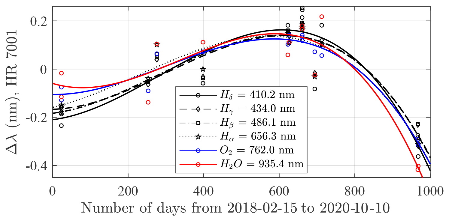
Figure 8 SPST09 spectral drift over several seasons for the stellar hydrogen absorption lines of the Balmer series and the atmospheric O₂ and H₂O lines. The curves are third-order polynomial fits.

A third broadband consequence of the spectral drift results from the stellar-magnitude spectra being generally characterized by a significant positive spectral slope, over the 400–1100 nm range, for both A- and B-class stars, (see Figs. 9a and 10a, respectively). This shift in wavelength transforms into a spectral incoherency between the catalogued M₀ values and the measured signal. The M₀ bias corresponding to the positive-slope stellar spectrum in Fig. 9a for ±0.5 and ±1 nm shifts is illustrated in Fig. 9b. These results indicate that the maintenance of photometric bias values below 0.01 magnitudes requires a spectral calibration within 1 nm (excluding the case of strong water vapour absorption in the NIR region). The same exercise is presented in Fig. 10 for the early-type B star. While there are individual channel differences with respect to the class-A star, the broad δM₀ results are similar because the M₀ slopes are similar.

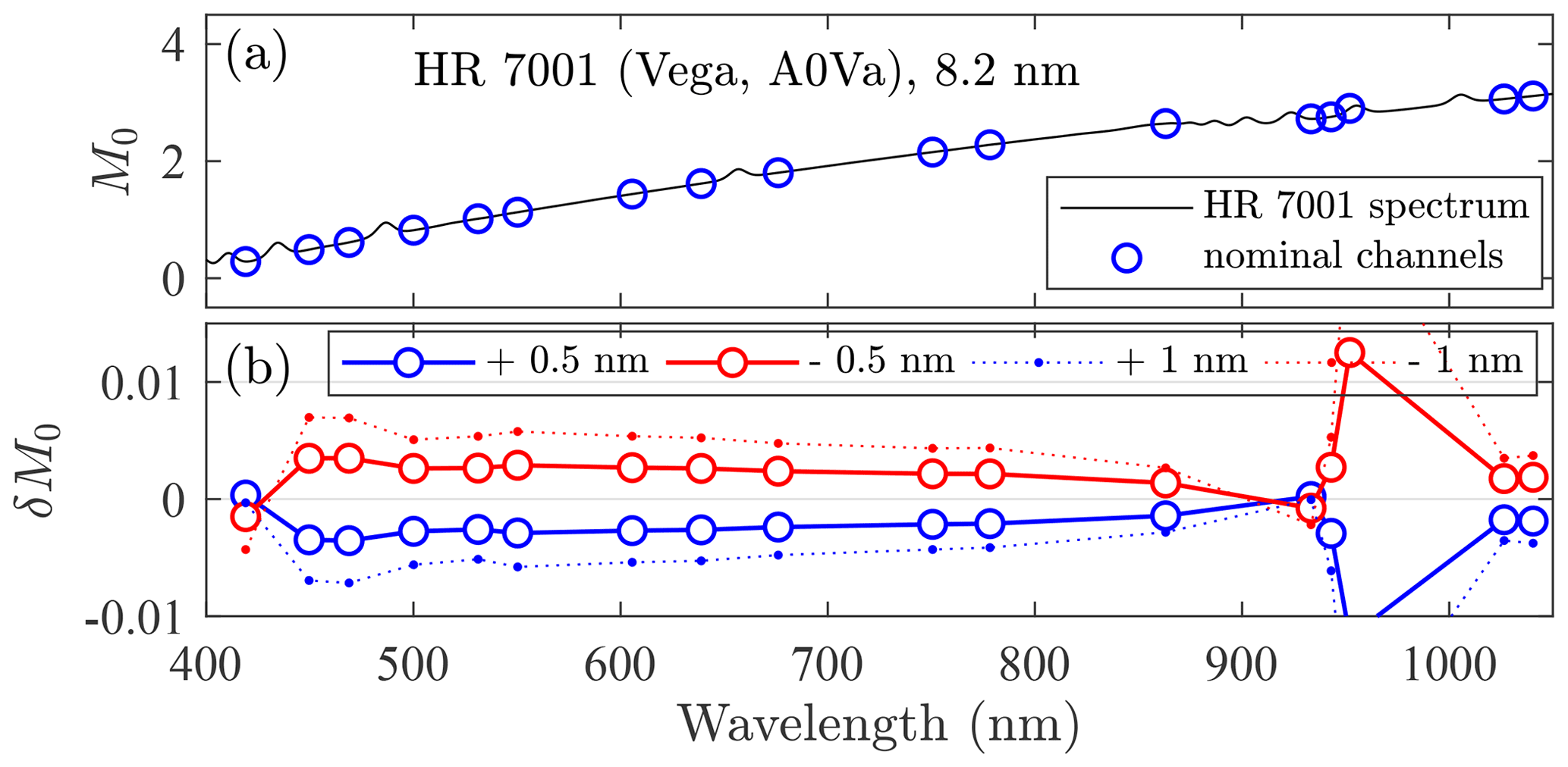
Figure 9 Bandwidth mismatch error for an A-class star (Vega, HR 7001), as a consequence of a spectrum shift.

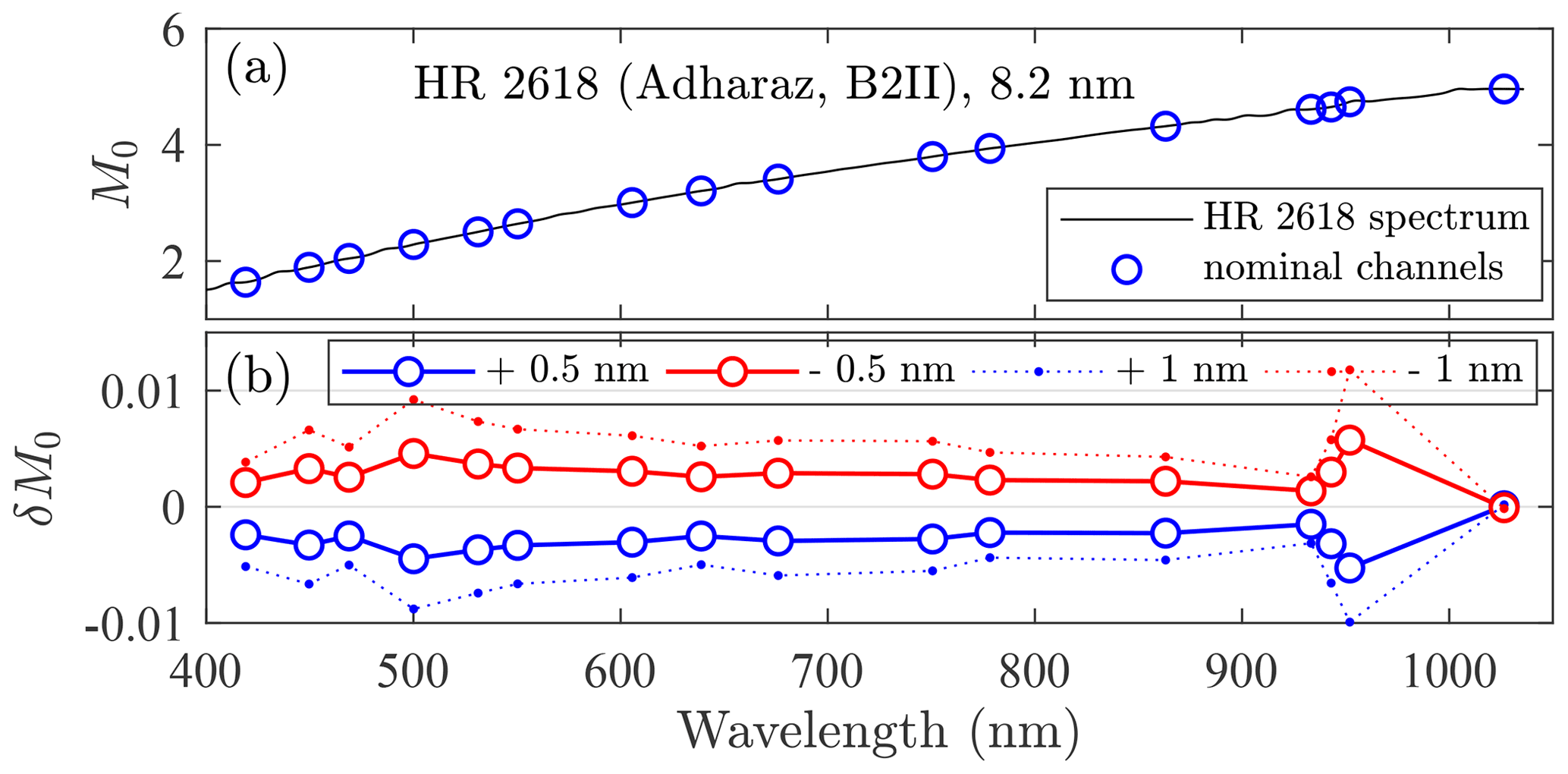
Figure 10 Bandwidth mismatch error for an (early-type) B-class star (Adharaz, HR 2618), as a consequence of a spectrum shift.

As long we employ the same class (similar spectral signatures) for both high- and low-Δ TSM stars, any spectral drift is mitigated in real time (i.e. similar δM₀ trends produce common biases; thus, the type of bias mitigation discussed in the case in Fig. 4 will prevail). While the bias in the OSM case will be initially absorbed into the calibration constant, any additional drift will progressively propagate into post-calibration δ_τ error. Based on the analysis in Fig. 8, an annual spectral calibration (preferably at the beginning of the observation season) will likely ensure that the spectral drift is constrained to values ≲0.5 nm, with negligible effect on the measurement accuracy. Our experience indicates that the six absorption lines employed in the development of Fig. 8 are sufficient to adequately characterize the spectral shift of all of the starphotometer channels. The radial velocity (stellar centre of mass moving away or towards an Earth-bound observer) of our Eureka stars, as retrieved from Wenger et al. (2000), lead to a 0.15 nm maximum Doppler spectrum shift at 1000 nm and a maximum Doppler spectrum shift of 0.06 nm at 400 nm among our stars. Therefore, this effect can be neglected during spectral calibration.

4.4 Alternative catalogues

An M₀ catalogue whose bandwidths match those of the instrument is preferred in order to avoid bandwidth mismatch errors. One natural approach would be to generate an S₀ catalogue by calibrating the starphotometer at a high-altitude site. A single calibration site may not, however, yield a sufficient number and class diversity of S₀ values (i.e. a sufficiently comprehensive catalogue of stars) to satisfy the starphotometry requirements of a given operational starphotometer site. For spectrometer-based starphotometers, it is necessary to retrieve S₀ at all available spectrometer channels (not just the nominal operational channels), as the spectral drift calculations need to be done at the highest resolutions. This S₀ catalogue can then be transformed into a corresponding M₀ catalogue by first resampling HST M₀ values of a selected reference (Vega or Sirius) to the spectrometer resolution and then employing Eq. (14) to compute C. With that HST-derived value of C in hand, the same equation can be rearranged to yield $M_{\mathrm{0}}=C+S_{\mathrm{0}}$ values for all of the other stars. Accurate C values and spectral calibration may also be obtained in the laboratory with the help of a halogen calibration lamp (Paraskeva et al., 2013) or by undertaking simultaneous measurements on-site with a co-located calibrated instrument.

The alternative to an instrument-specific catalogue is to use a general purpose high-resolution spectrophotometric catalogue, from which one can synthesize magnitudes at any bandwidth (as we did with the HST spectra). Given the maximum bandwidth mismatch errors found in the Pulkovo catalogue (∼0.04 in Fig. 6b for standard channels, at 8.2 nm bandwidth), we estimate that a catalogue with about a 1 nm bandwidth (i.e. about a factor 10 less) would be enough to limit the errors to <0.01. We note that the generally sub-0.01 mismatch errors estimated for a 1 nm spectrum shift (Figs. 9b, 10b) are not inconsistent with this affirmation. In general a higher-resolution catalogue such as the HST catalogue, with its 1 Å resolution, would be preferred. It is, however, surprising that there are no existing high-resolution, near-UV to NIR, spectrophotometric catalogues that achieve 1 % accuracy (Kent et al., 2009) for bright (V<3) stars. The stars observed by professional astronomers are usually much fainter (V>6) in order to avoid saturating the detectors. This may explain the lack of interest from the astronomical community in improving the absolute spectrophotometry of bright stars. An effort to address this situation was pursued by Le Borgne et al. (2003), with their release of the STELIB catalogue. However, we identified large biases in the UV/blue part of the STELIB spectra (Fig. 11) in comparison with the HST NGSL catalogue. The fact that the Pulkovo catalogue also has the largest bias in that range (Fig. 4) suggests a recurring issue for catalogues generated from ground-based observations (perhaps due to the higher optical depth in the blue and the deficient compensation for aerosol contributions) and, accordingly, that an accurate catalogue must be of extraterrestrial origin. Most of the ground-based measurements are focused on achieving a 1 % accuracy using broadband photometry (Stubbs and Tonry, 2006). It is noteworthy, however, that Zhao et al. (2012) reported a new spectrophotometric (high-spectral-resolution) catalogue (including our entire bright-star dataset) derived from LAMOST (Large Sky Area Multi-Object Fiber Spectroscopic Telescope) measurements that approached the same 1 % accuracy. The spectral resolution and bandwidth of this catalogue are variable but are always sub-nanometre. The spectral range extends over most of our spectrum but, unfortunately, not beyond 900 nm. A novel future approach for improving the ground-based catalogues would be to employ an accurately calibrated satellite light source in order to perform stellar differential photometry (Albert, 2012; Peretz et al., 2019).

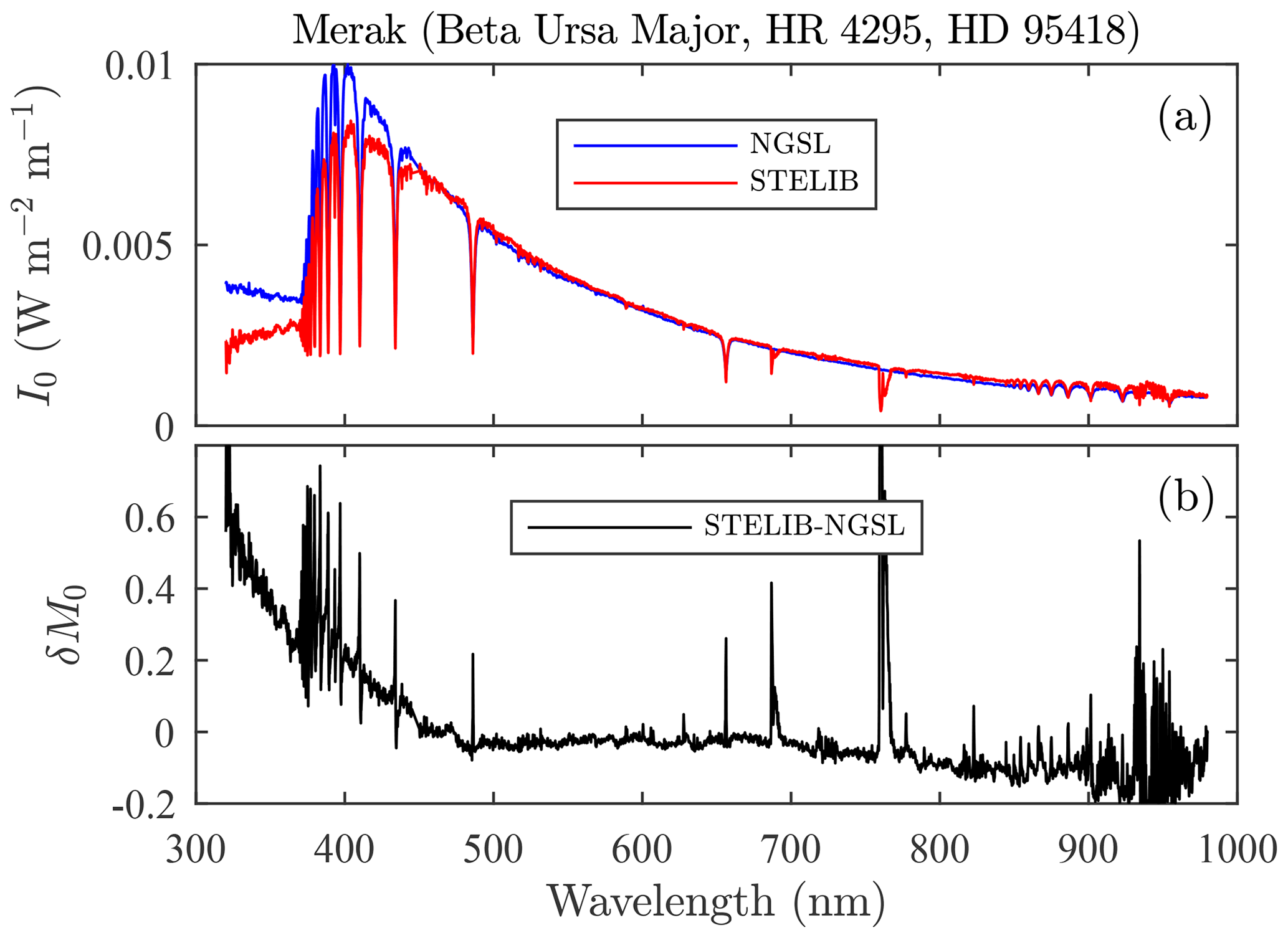
Figure 11 Spectrophotometric comparison of the STELIB catalogue with respect to the HST NGSL (a). Important bias are seen in the UV, and a much weaker bias is seen in the IR (b).

As an alternative to satellite-based catalogues, the recent ACCESS (Absolute Color Calibration Experiment for Standard Stars) rocket project (Kaiser and Access Team, 2016) was also a promising initiative, given the project's mandate to perform high-spectral-resolution photometry near the top of the atmosphere. Unfortunately, their list of V<3 bright stars is limited to Sirius and Vega. Another recent initiative is the NIRS STARS campaign (Zimmer et al., 2016), whose mandate is to produce a bright-star spectrophotometric catalogue using lidar measurements to remove the atmospheric contribution. However, once again, the brightest stars (V<3) are largely excluded from consideration. The most promising option is the use of Global Ozone Monitoring by Occultation of Stars (GOMOS) satellite-based star observations (Kyrölä et al., 2004). This sensor employs high-resolution (1.2 and 0.2 nm, depending on the spectral bands) limb starphotometry to retrieve ozone and other atmospheric components from space. Its off-limb measurements, performed before each limb scan, can be used to build an exoatmospheric spectrophotometric catalogue (Ivănescu et al., 2017). Unfortunately, the GOMOS spectral ranges of 250–675, 756–773, and 926–952 nm do not cover our entire 400–1100 nm spectrum. They do, however, cover the problematic spectral ranges experienced in ground-based measurements (the UV/blue and across the O₂ and the H₂O absorption bands). The missing portions of the starphotometer spectra can be filled in by fitting the STELIB, LAMOST spectra, synthetic spectra (Rauch et al., 2013), or averaged star-type spectra (Pickles, 1998) to the GOMOS measurements.

Nevertheless, the broadband photometric stability of bright stars remains an open question (as emphasized in Appendix B) and requires investigation. A uniform photometric variation over the entire observed spectrum may, however, be less critical than a non-uniform one. In an example of the latter case, star temperature variations would lead to spectral distortions with potential impacts on aerosol retrievals. The analysis of the GOMOS measurements should enable a characterization of spectral variability. If, however, an insufficient number of stable V<3 stars are found (i.e. stars with differential M₀ variations of <0.01 between channels), the use of fainter stars may be necessary: this would require the deployment of a larger starphotometer telescope. In the short term, we will continue to employ the Pulkovo catalogue spectra for the operational M₀ values of our star dataset. However, we will use a synthesized 8.2 nm version, over the available spectral range, to mach our starphotometer bandwidths.

5 Air mass (x) accuracy

Systematic errors in the calculation of the air mass m (or alternatively x) can be significant (see, for example, Rapp-Arrarás and Domingo-Santos, 2011, for a review of analytical air mass formulae). The following operational equation characterizes m, in a spherically homogeneous, dry-air atmosphere with an accuracy of better than 1 % at m=10 (Hardie, 1962):

$$\begin{array}{}\text{(35)}& \begin{array}{rl}m& =\sec z-\mathrm{0.0018167}(\sec z-\mathrm{1})\\ & -\mathrm{0.002875}(\sec z-\mathrm{1}{)}^{\mathrm{2}}-\mathrm{0.0008083}(\sec z-\mathrm{1}{)}^{\mathrm{3}},\end{array}\end{array}$$

where z is the apparent zenith angle (the zenith angle of the refraction-dependent telescope line of sight). This expression only departs significantly from the plane-parallel expression of m=secz at values of m>5. If the target star position is computed using astronomical data rather than a measured instrumental mount position, it is more appropriate to use the true zenith angle (z_t) formula of Young (1994). The computation of z_t can be effected using star coordinates, site location, and time. It ensures an associated maximum 0.0037 air mass error at the horizon (with respect to calculations made on a standard mid-latitude atmospheric model).

One should note that the air mass depends slightly on the vertical structure of the atmosphere (Stone, 1996; Nijegorodov and Luhanga, 1996): an effect which is particularly distinctive in a polar environment. The relative errors due to such environmental variations are, however, below 0.2 % up to $z\simeq \mathrm{82}{}^{\circ }$ (m≃7) and below 1 % at $z\simeq \mathrm{87}{}^{\circ }$ (m≃15) (Tomasi and Petkov, 2014). Differences in air mass associated with different atmospheric constituents (Tomasi et al., 1998; Gueymard, 2001) have a negligible impact on the observation accuracy of starphotometry.

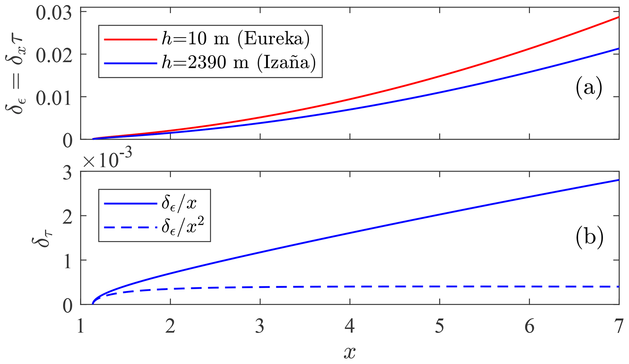
In spite of the generally high accuracy associated with air mass expressions, the air mass error can be significant if the recorded timestamps are inaccurate. Stars targeted by our starphotometers are re-centred between several (3–5) consecutive exposures: a process that is of variable duration (usually 20–40 s). The air mass associated with the mean of all of the measurement times (the one reported) may differ from the air mass associated with the mean observation time (the weighted mean time where the weights are exposure duration times). A δ_x error in x, induced by a δ_t time error, is equivalent to a measurement error δ_ϵ≡δ_xτ (Eq. 33). Figure 12 shows the variation in δ_ϵ with altitude (for hypothetical observation sites at different elevations), for a ${\mathit{\delta }}_t=+\mathrm{30}$ s case (i.e. time overestimation leading to δ_x>0 for a descending star) at λ=400 nm, and for three different air masses in a Rayleigh atmosphere (the condition of molecular scattering domination; see Bucholtz, 1995, for the optical parameterization of a Rayleigh atmosphere).

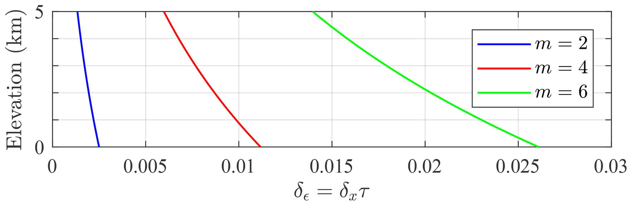
Figure 12 Assessment of stellar-magnitude errors associated with air mass miscalculation errors due to a time delay error (δ_t) of 30 s in a Rayleigh scattering atmosphere and as a function of the hypothetical elevation of a starphotometer site.

The variation in δ_ϵ with x is shown in Fig. 13a for observations at 10 m (Eureka elevation) and 2360 m (Izaña observatory elevation). The real x variation at Eureka is weak (near the poles, stars carve out sky tracks that vary little with respect to zenith angle). The δ_ϵ variation, for unrestricted variation in x (up to x=7), will be comparable for both sites. Figure 13b shows the corresponding δ_τ error for Izaña (solid blue line) growing linearly with x, and a dominating x² dependency demonstrated by the saturation of the ${\mathit{\delta }}_{\mathit{ϵ}}\left(x\right)/x^{\mathrm{2}}$ curve (dashed blue line). For this simulated δ_t = 30 s case, δ_τ<0.01 even at large x. However, the computer time may typically drift by about 1 min yr⁻¹ (Marouani and Dagenais, 2008): a scenario where δ_τ would be significant. Thus, the computer time has to be corrected weekly, if not daily (using, for example, a GPS time server).

Figure 13 (a) Assessment of accuracy associated with air mass miscalculation errors for a descending star (same conditions as Fig. 12). Panel (b) shows δ_τ in the case of Izaña site (where ${\mathit{\delta }}_{\mathit{\tau }}=\mathit{\tau }{\mathit{\delta }}_x/x={\mathit{\delta }}_{\mathit{ϵ}}/x$); ${\mathit{\delta }}_{\mathit{ϵ}}/x^{\mathrm{2}}$ shows δ_x dependency in x².

6 Observation (S) accuracy

6.1 Heterochromaticity

Wideband optical depth calculations using starlight as the extinction source were first described in Rufener (1964) (in French). A comprehensive description by Golay (1974) (pp. 47–50) affirms that non-linear, wideband radiation detection effects are negligible in terms of S estimation for spectral bandwidths narrower than 50 nm. The error associated with this non-linear component is about the squared ratio between the bandwidth and the central wavelength, i.e. $(\mathrm{\Delta }\mathit{\lambda }/\mathit{\lambda }{)}^{\mathrm{2}}$ (Rufener, 1986). A bandwidth of less than 40 nm is then sufficiently small to achieve optical depth errors <0.01 at 400 nm. These optical depth (heterochromaticity) errors should be well below the negligible value of 0.001 for our sub-10 nm starphotometer-channel bandwidths.

6.2 Log-normal fluctuations

The optical depth retrieval, as expressed by Eq. (23) or (25), is based on computing the instrumental magnitudes S through the logarithm of the measured star signal F. However, before doing so, one performs an arithmetic mean $\stackrel{\mathrm{‾}}{F}$ over several consecutive exposures. As F is subject to log-normal fluctuations induced primarily by scintillation effects (Roddier, 1981), one should characterize its probability distribution in terms of its geometric mean $\stackrel{\mathrm{‾}}{\log F}$ and its geometric standard deviation σ_log F. The corresponding bias, called the “misuse of least-squares” by Young (1974), is given by

$$\begin{array}{}\text{(36)}& {\mathit{\delta }}_{\log F}=\log \stackrel{\mathrm{‾}}{F}-\stackrel{\mathrm{‾}}{\log F}={\mathit{\sigma }}_{\log F}^{\mathrm{2}}/\mathrm{2}\end{array}$$

(a classical relationship between the geometric and arithmetic means). From Eq. (16) and the general definition of a standard deviation, δ_S=2.5δ_log F and, similarly, σ_S=2.5σ_log F. The bias then becomes

$$\begin{array}{}\text{(37)}& {\mathit{\delta }}_S={\mathit{\sigma }}_S^{\mathrm{2}}/\mathrm{5}.\end{array}$$

As a single OD measurement is effectively the arithmetic mean of three to five measurements, observation fluctuations with σ_S>0.22, which we basically never experienced (even with large air masses), would lead to δ_S>0.01. One can conclude from Eq. (32) that xδ_τ<0.01; thus, the above-mentioned issue is negligible in starphotometry.

6.3 Forward scattering

Forward scattering into the photometer FOV by large atmospheric particulates (notably cloud particles) increases the magnitude of S, thereby inducing an underestimate of the optical depth. This “forward-scattering error” can be estimated with the single-scattering expression⁸

$$\begin{array}{}\text{(38)}& {\displaystyle \frac{{\mathit{\delta }}_{\mathit{\tau }}}{\mathit{\tau }}}=\stackrel{\mathrm{‾}}{\mathit{\omega }}\cdot P\mathrm{\Delta }\mathrm{\Omega },\end{array}$$

where $\stackrel{\mathrm{‾}}{\mathit{\omega }}$ is the single scattering albedo (or SSA) and PΔΩ is the integral of the normalized scattering phase function P over the angle $\mathrm{\Omega }=\mathrm{FOV}/\mathrm{2}$ (Shiobara et al., 1994). Figure 14 shows a variety of forward-scattering error calculations obtained using Eq. (38) at a wavelength of 400 nm. The red curve represents a typical biomass burning aerosol example (Qie et al., 2017) based on P given by the widely used Henyey–Greenstein (HG) phase function (Zhao et al., 2018). It underscores its negligible forward-scattering error on any practical FOV size.

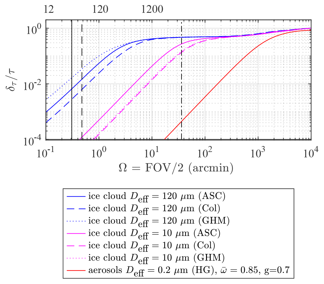
Figure 14 The relative forward-scattering error for typical aerosols and ice clouds, as a function of the half field of view. The vertical black lines correspond to SPST09/C11 (solid line), SPST05/M703 (dashed line), and Cimel sun/moon photometers (dot-dashed line). The acronyms in parentheses specify the phase function model.

For ice crystals, $\stackrel{\mathrm{‾}}{\mathit{\omega }}$ is practically unity. Two ice crystal effective diameters were employed: 10 µm (non-precipitating clouds, magenta curves) and 120 µm (precipitating clouds, blue curves). Three crystal habit models were employed to represent the variation in the bulk phase function with crystal habit (from the computations of Baum et al., 2014): severely roughened aggregates of solid columns (ASC, solid curves, typical in the High Arctic), severely roughened solid columns (Col, dashed curves), and general habit mixture (GHM, dotted curves). Several relevant instruments are represented by vertical black lines in Fig. 14: SPST09/C11 (solid), SPST05/M703 (dashed), and the Cimel sun/moon photometers with a 1.2^∘ FOV (dot-dashed).

The computations in Fig. 14 assume that the contaminating particles (those that induce the FOV scattering effect) are also the particles that one seeks to detect. These ${\mathit{\delta }}_{\mathit{\tau }}/\mathit{\tau }$ computations still apply when the contaminating particles differ from the particles to be detected as long as the FOV effect of the contaminating particles dominates the FOV effect of the latter. For example, the effect could be dominated by low-OD ice clouds while one seeks to detect fine-mode (FM) aerosols of significantly higher OD. When measurements are made using Cimel-like instruments in the presence of clouds with ${\mathit{\delta }}_{\mathit{\tau }}/\mathit{\tau }$ above 0.15 (the intersection of the dot-dashed Cimel line with the dashed magenta ice cloud curve in Fig. 14), the δ_τ<0.01 requirement can only be fulfilled for COD <0.07. If the clouds are thicker than that (which is generally the case), cloud screening is required to ensure an accurate AOD. In the case of our starphotometers, these errors are negligible in the presence of non-precipitating ice clouds (D_eff=10 µm in Fig. 14). Even in the case of precipitating clouds (D_eff=120 µm in Fig. 14), the SPST09/C11 instrument, for which ${\mathit{\delta }}_{\mathit{\tau }}/\mathit{\tau }\sim \mathrm{0.01}$, still provides the required accuracy as long as τ<1.

The possibility of exploiting the unique nature of very small FOV starphotometry to characterize AODs in the presence of thin cirrus clouds⁹ merits further consideration, as the spectral deconvolution algorithm (SDA) technique (O'Neill et al., 2003) enables the separation into FM and CM (coarse-mode) ODs. One cannot aspire to separate out CM AODs from cirrus ODs without some degree of independent information, whereas separating out FM AOD (the dominant aerosol component) is entirely feasible for starphotometry.¹⁰

6.4 Night sky background

Airglow and potentially aurora can be important contributors to the night sky background (see Chattopadhyay and Midya, 2006, on the importance of airglow). Their high-frequency temporal and spatial variability (Dempsey et al., 2005; Nyassor et al., 2018) complicates their elimination in a background subtraction process. This can lead to significant optical depth systematic errors. Their spectra are similar: in particular, both exhibit a strong 557.7 nm neutral oxygen ([OI]) green emission line, whose intensity is used for classification of auroral strength. Unique signature features of each phenomenon are those due to OH-band emissions in the case of airglow and N₂ (first positive system) emissions in the case of aurora (Chamberlain, 1995). The emission line intensities are usually expressed in rayleigh (R) units (which are effectively a measure of directional panchromatic radiance, as per Baker, 1974), with the airglow exhibiting typical 557.7 nm (line-integrated) values of ∼0.25 kR. The International Brightness Coefficient (IBC) is employed to discriminate four aurora classes: IBC1 = 1 kR (brightness of the Milky Way); IBC2 = 10 kR (brightness of thin moonlit cirrus clouds); IBC3 = 100 kR (brightness of moonlit cumulus clouds); and IBC4 = 1000 kR (provides a total illumination on the ground equivalent to full moonlight) (Chamberlain, 1995). We note that the assessment of the accuracy errors for those classes may help to infer the effect of moonlight and moonlit clouds too.

Figure 15a shows the aurora classes' emission density spectra (rayleigh per unit wavelength) converted to the 8.2 nm bandwidth of our starphotometers. The airglow data (the black solid curve) represent tropical night-time observations made by Hanuschik (2003). These include zodiacal light (sunlight scattered by dust from the solar system ecliptic plane). Accordingly, the actual airglow emissions should be even weaker. The aurora density spectra (the coloured solid curves) are a compilation of observations from Jones and Gattinger (1972), Gattinger and Jones (1974), and Jones and Gattinger (1975, 1976). Their spectra were adjusted to produce three curves that represent the first three IBC levels. Their common continuum (without respect to aurora class) is adjusted to 8 R Å⁻¹, the minimum value proposed by Gattinger and Jones (1974).

Figure 15 (a) Typical emission density spectrum for airglow and aurora. (b) Corresponding optical depth error in the presence of uncorrected emission contributions: ${\mathit{\delta }}_{\mathit{\tau }}={\mathit{\delta }}_F/F$ (from Eq. 32 for m=1), representing the ratio of emission to a Vega spectrum dimmed to V=3 and attenuated in a Rayleigh atmosphere. When observing a V=0.5 star, the corresponding aurora IBC types can be one class brighter to achieve the same optical depth errors. The red dots show comparative V=3 results for the (larger FOV) M703 instrument (see text for details).

Figure 15b enables an appreciation of airglow and aurora effects on starphotometer measurements. It shows the ratio of those spectra to the Vega spectrum (artificially attenuated to magnitude V=3, the faint limit of our star dataset). The resulting estimates of optical depth error (Eq. 32 converted to observational error xδ_τ of Eq. 33), in the presence of uncorrected emission contributions, correspond to the throughput of the C11. Optical depth errors for the M703 (shown only for the IBC2 case of red dots) are the result of the M703 (FOV-filling IBC2) flux being 2.4 times larger than that of the C11, i.e. the ratio of their solid angles, $(\mathrm{57.3}/\mathrm{36.9}{)}^{\mathrm{2}}$. We note that, in spite of the fact that the C11 emission spectra are significantly higher in the NIR spectral region, they are, except for the IBC3 case, generally less than 1 %. Short-term airglow variability induced by air density fluctuations engendered by gravity waves may occur (Nyassor et al., 2018). However, Fig. 15b indicates that typical airglow conditions have a negligible error contribution. Even at twilight, when the sodium emission lines, at 589.3 nm, can be enhanced by a factor of 5 (i.e. the “sodium flash” reported by Krassovsky et al., 1962), the potential accuracy error remains negligible.

On the other hand, the aurora is characterized by a much higher temporal and spatial variability (Dempsey et al., 2005). Moreover, the aurora shown in Fig. 15 is of the green type (i.e. main visible line at 557.7 nm), but one may have other types too – the most common being red, with the main visible line at 630 nm. Therefore, one may also encounter spectral variation. Such variation may induce significant departures from the nominal emission background spectra shown in Fig. 15a. Considering the results in Fig. 15b, the worst estimation of these variations, the optical depth error remains well below 0.01 for the C11 telescope, even when observing a weak V=3 star during an IBC2 aurora (solid red line). An IBC3 Aurora can, given that a (factor of 10) IBC class change is equivalent to a magnitude change of 2.5, be accommodated by employing a sufficiently bright star: the IBC3 representation for a V=0.5 star will decrease to the red (sub-0.01 error) IBC2 curve in Fig. 15b. Fortunately, given the current location of Eureka in the auroral oval (Vestine, 1944), IBC3 aurora will only be seen occasionally near the horizon. Therefore, the accuracy errors in Fig. 15b will only appear at air masses above 5. However, this may change in the coming decades, given the recent fast pace of the migration of the magnetic pole (Witze, 2019; He et al., 2020).

The IBC definition also provides a way to infer ${\mathit{\delta }}_F/F$ errors associated with the presence of thin moonlit clouds by simply arguing that the red IBC2 curve in Fig. 15b also applies to the IBC2 analogy of “thin moonlit cirrus clouds”. By definition, the δ_F spectrum for such a case corresponds to the IBC2 radiance in Fig. 15a. The F value for a V=0 star in a thin-cloud atmosphere can be modelled, in an order-of-magnitude fashion, by assigning a value of τx=3 to Eq. (21). Using this attenuated star signal as a rough model for the IBC2 moonlit clouds analogy, we employ the same equation to show that the V=0, cloud-attenuated star magnitude is equivalent to an unattenuated (τ=0) V=3 star. In other words, the same F is used to obtain the red ${\mathit{\delta }}_F/F$ curve in Fig. 15b, although with the added rider that the exoatmospheric star was a V=0 star. Accordingly, the acceptability of the sub-10⁻² red error curve in Fig. 15b applies to the moonlit cloud IBC2 analogy, although for a V=0 star. Actually, given the strong snow albedo in the Arctic, thin-cloud brightness may even exceed IBC2 brightness during full moon conditions. However, quantitative assessment of optical depth errors related to moonlit and twilight-lit sky brightness, especially in cloudy situations, would require the development of a radiative transfer model informed by starphotometer background measurements. Given the complexity and specificity of such endeavour, this will be addressed in a future study.

The typical polar wintertime night sky background spectrum at Eureka (in terms of catalogue photometric system magnitude per square arcsecond) is shown in Fig. 16a for two different times: midday (magenta curve, local time) and evening (black). The evening sky is darker and approaches the detection limit of our instrument (as made evident by its noisier profile). This detection limit may be the reason for the difficulty in identifying the aforementioned aurora and airglow lines in the visible range. However, an omnipresent weak line, unassociated with any major aurora emission lines, is noticeable around 440 nm (436–445 nm band). Some absorption lines can also be identified: 532 nm, probably due to O₄ (Orphal and Chance, 2003), and 663 nm, probably due to NO₃ (Orphal et al., 2003). The midnight sky is expected to be even darker (higher visible magnitude). One also notices a brighter infrared spectrum that is rather constant throughout the day, confirming the J-band measurements of Sivanandam et al. (2012). This may be associated with the airglow OH lines but is a factor of ∼10 higher than estimated in Fig. 15b. The evening sky background with respect to a magnitude V=3 star (simulated by dimming Vega) exceeds the 1 % mark beyond 900 nm (red curve in Fig. 16b). With respect to a magnitude V=0 star (Vega, blue curve), the evening sky background remains below the 1 % mark in the starphotometer spectral range (i.e. <1050 nm). This indicates that accurate measurements, in the case of weakly radiating (V>1) stars, can only be achieved by applying a reasonably accurate background subtraction for wavelengths larger than 1000 nm.

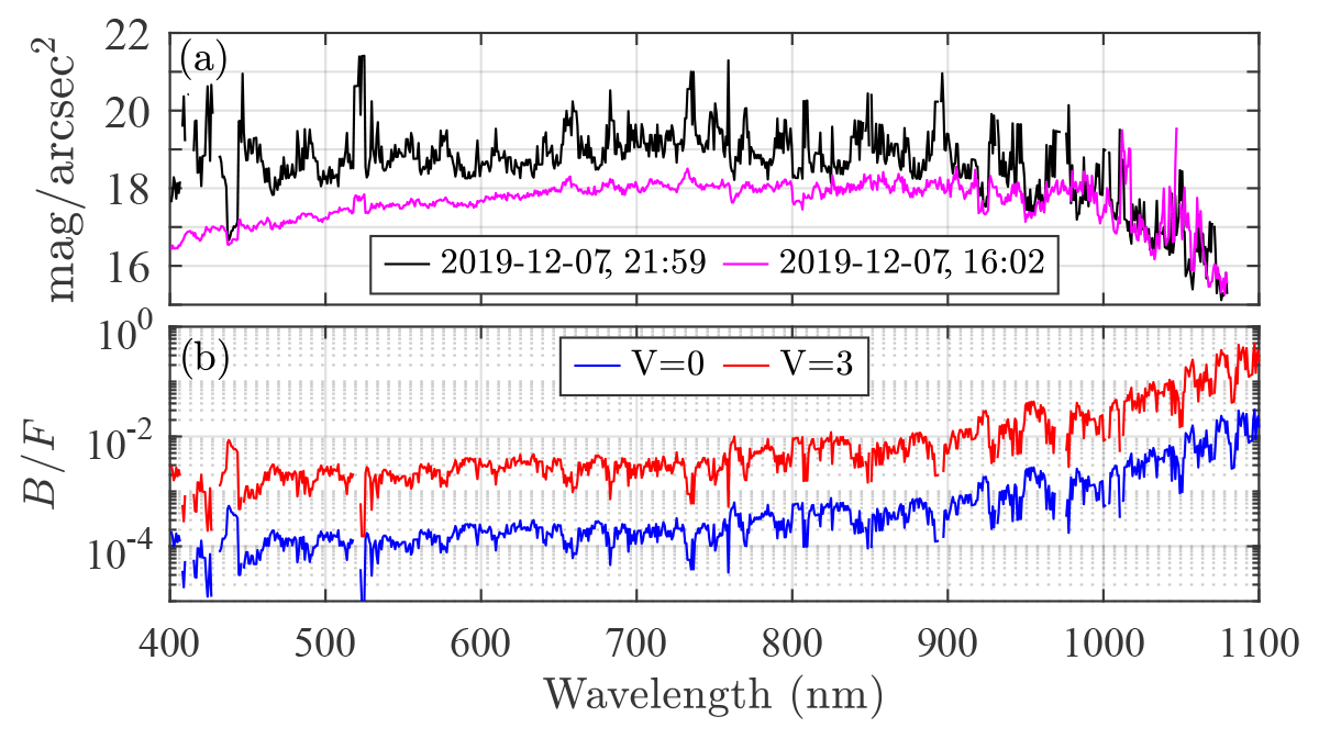
Figure 16 (a) Night sky background spectrum, measured with the Eureka SPST09/C11 (in the Pulkovo catalogue photometric system) at midday (magenta curve) and in the evening (black curve) during polar night. (b) Ratio of background to star flux for the evening sky and for two star magnitudes: Vega at V=0 (blue curve) and a dimmed Vega at V=3 (red curve). Times are UTC.

7 Calibration parameter (C) accuracy

The accuracy of the calibration parameter C retrieval is dependent on the performance of the calibration procedure and will accordingly be addressed in a separate study. C accounts for the optical and electronic throughput: here, we assess the instrument instability or degradation that may alter it.

7.1 Starlight vignetting

One way to get throughput degradation is by losing flux outside the boundary of the FOV (commonly called vignetting) due to focusing errors (blurring), off-axis star-centring errors, or because the FOV is simply too small (design errors). The instrument was originally built for the M703 telescope specifications. The smaller FOV of the C11 telescope (almost half that of the M703) is at greater risk of focusing errors, particularly at Eureka, where the starspots are larger (Fig. 2). An analysis of the impact of design shortcomings on both instruments is an instructive exercise. Figure 17 illustrates the effect of defocusing the optical train within the context of the associated OD errors (case of the C11 telescope) and of star-centring errors (cases of both the C11 and M703 telescopes). The fitted curves, which are well modelled by an $a|s{|}^b$ equation, are only employed to estimate the error variation for low OD (where the density of measurement points is prohibitively small). For the focusing error, the negative and positive s values refer to the starspot shift, in steps of the focusing stage (the adjustable unit that controls the focusing of the star photometer at ∼1.36 mm per step along the axis or, equivalently, ∼10 arcsec per step of angular increase in the confusion circle), before and after passing through the on-focus position. For the centring error, they refer to the spot shift, in pixels of the high-resolution camera, before and after passing through the on-axis position.

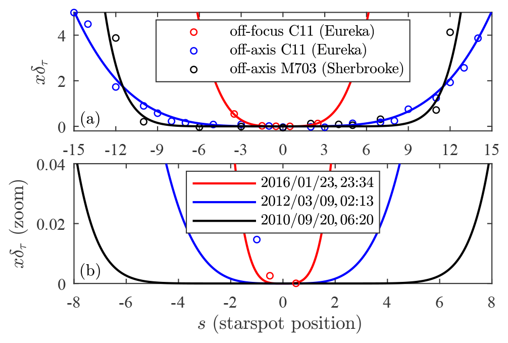
Figure 17 Optical depth increase induced by throughput degradation due to misalignment: star focusing error (red for C11) and centring error (blue for C11 and black for M703). For focusing, the positions (s) represent focusing stage steps (at ∼10 arcsec per step increase in the confusion circle); for centring, they represent high-resolution camera-binned pixels, at 3 arcsec per bin for M703 and 2 arcsec per bin for C11. Panel (a) shows the data and $a|s{|}^b$ fit; panel (b) shows the same fit as panel (a) but zoomed-in to low OD. (The measurement date and UTC time are indicated in the legend of panel b.)

Our focusing stage employs a continuously driven motor that is subject to electronically controlled steps. Those steps represent approximately the same distance along the optical axis, based on a fixed driving time interval. The best that can be achieved is a half-step focus, for which the flux loss, in the C11 case, is a negligible ∼0.02 %. In the absence of an automatic focusing procedure, the focus has to be checked and adjusted manually whenever there is an important temperature variation. This may happen because of weather changes or as the result of opening the dome (with significant optical impacts up to 1 h after the opening). Based on our Arctic experience, the focus must be corrected by one focus step for each 10 ^∘C change in temperature: if this correction is performed, the flux loss is a negligible 0.35 %. Any focusing errors larger than that will significantly affect the optical depth estimation (Fig. 17b).

Star centring is based on an automatic tracking procedure that ends once a specified centring tolerance δ_c is satisfied (where δ_c is an input parameter required as part of the starphotometry measuring sequence). Such a tolerance has to be small enough to ensure that, during the subsequent measurement, the star still remains in the accepted centring range, despite any drift due to its natural jitter (spot wandering due to the air turbulence). On the other hand, a faster centring procedure can be achieved using a larger tolerance. Therefore, there is a trade-off to be made between these two requirements. This is investigated in Appendix C by taking the constraints posed by the FOV into account. We show, for a perfectly aligned star, that the maximum seeing that the FOV can accommodate is 16.7 arcsec, for our C11 Arctic telescope. This is borderline at m=5 in Fig. 2 (long-exposure case). Obviously, this somewhat too small FOV is a design shortcoming that can be fixed, for example, with a larger limiting diaphragm.

In order to assess the accuracy, we employ the calculations of Appendix C to transform the Arctic starspot sizes in Fig. 2 into the corresponding observation errors in Fig. 18. The black curve represents a systematic throughput degradation due only to the flux loss at the edges of the starspot. Such degradation characterizes the case of a perfectly centred (δ_c=0 arcsec) short-exposure starspot (ω_s).

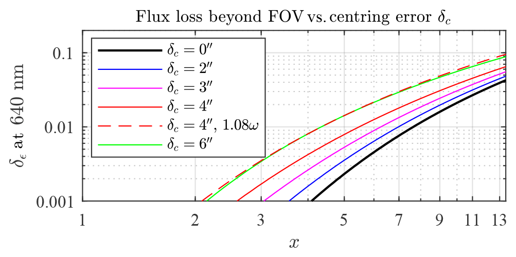
Figure 18 Observation error due to throughput degradation at Eureka when using the SPST09/C11 system. This error is the result of a FOV that is too small combined with a centring error (see the main text for details).(Note that “′′” denotes arcseconds in this figure.)

The coloured curves account for the attendant error due to different centring tolerance choices (δ_c=2 arcsec, 4 arcsec, and 6 arcsec). We compute them by quasi-quadratically summing (with a $\mathrm{5}/\mathrm{3}$ Kolmogorov turbulence exponent) the natural jitter contribution and the position uncertainty inside the tolerance zone, i.e. $({\mathit{\sigma }}_{\mathit{\theta }}^{\mathrm{5}/\mathrm{3}}+{\mathit{\delta }}_{\mathrm{c}}^{\mathrm{2}}{)}^{\mathrm{1}/\mathrm{2}}$, with σ_θ from Appendix C. One has to keep in mind, however, that those calculations are based on the blue linear fit of data points used in Fig. 2. The possible variations about that line can be estimated inasmuch as the short exposures indicate a standard deviation of 5 %–10 %. This is about the 5 % difference between the long- and short-exposure spot sizes in the Kolmogorov turbulence case, as computed in Appendix C (the approximation ${\mathit{\omega }}_{\mathrm{s}}\simeq \mathrm{0.95}\cdot \mathit{\omega }$ following Eq. C2). However, for the purposes of our error modelling, we retained an empirical 8 % standard deviation case. Accordingly, the ω_s values (of a Gaussian distribution in ω_s) may be greater than ω values 33 % of the time (33 % of the Gaussian distribution that extends across the red line in Fig. 2 at 1 standard deviation from its blue line mean). This 1.08ω case is represented by the dashed red δ_c=4 arcsec curve in Fig. 18. The difference with respect to the plain red curve then accounts for the seeing variation. As it already exceeds our accuracy limit of 0.01 at x=4.4 (or m≃5), it represents the maximum acceptable δ_c for the constraints of our SPST09/C11 system.

7.2 Non-linearity

Non-linearity of detector response to incoming light flux is another source of systematic error. The onset of significant non-linearity conditions occurs at ∼8000 cnt s⁻¹ (i.e. $V=-\mathrm{0.47}$ with the C11 telescope – a level normally not reached by any star other than Sirius). If the sky brightness due to atmospheric scattering of sunlight is strong (at dawn or dusk at mid-latitudes, or for longer periods during seasonal shifts of the late and early winter in the Arctic), this limit will be exceeded. The culmination of the non-linearity is that, using our standard 6 s integration, the detector progressively approaches its saturation point at 2¹⁶ counts, or $\mathrm{65}\mathrm{535}/\mathrm{6}=\mathrm{10}\mathrm{922.5}$ cnt s⁻¹ (i.e. $V=-\mathrm{0.8}$ for C11). The consequence, as illustrated in Fig. 19, is an apparent decrease in star brightness (artificial reduction in the difference between the star and the sky measurements) with a corresponding increase in the computer value of the optical depth. The onset of non-linearity in the case of Vega (whose signal is ∼5000 cnt s⁻¹ at transit at Eureka) begins at a background (B) value of ∼3000 cnt s⁻¹ (at a total signal of ∼8000 cnt s⁻¹ as indicated above). One should never employ an instrument such as the C11 to make Sirius ($V=-\mathrm{1.46}$) attenuation measurements unless the OD >0.5. Data for which the signal exceeds 8000 cnt s⁻¹ should be discarded unless a subtraction process that accounts for the onset of non-linearity is applied.

Figure 19 Apparent decrease in star brightness (increase in magnitude M) as the sky background brings the detector into a non-linear regime. The star brightness has been corrected for sky brightness (the latter has been subtracted from the former). The separate background measurement (blue line) is not affected by the non-linearity of the detector as B<8000 cnt s⁻¹, but the sum F+B used to compute S is, leading to $M=S+C$, Eq. (13).

The sky background is strongly influenced by O₃ absorption. This is likely due to the multiple-scattering influence of the effective increase in the light path length (from the sub-horizon Sun to the telescope line of sight). This is underscored in Fig. 20, where we compare, in a relative fashion, the starphotometer sky background measurements with sky irradiance (daylight) computations at the bottom of a standard atmosphere for a solar zenith angle of 48.12^∘ “standard indirect solar reference spectrum” (ASTM-G173-03, 2012). The presumed multiple-scattering impact of ozone is almost negligible in the latter case, when compared with the starphotometer measurements for the sub-horizon Sun case. One should also note that other absorption bands, like O₂ at ∼760 nm or H₂O at ∼940 nm (for example), remain comparable. This means that the non-linearity, as well as saturation, happens first in the blue, leading to a distortion of the retrieved aerosols' optical depth spectrum.

Figure 20 Daylight sky background: standard ASTM G173-03 indirect solar reference sky irradiance spectrum (blue); scaled starphotometer background measurements at Eureka (18 February 2018, 10:33 LT, local time) to match the ASTM infrared level (red).

7.3 Delayed background

Unlike the majority of instrumentally related calibration-degradation influences discussed in this section, the particular problem of delays in background measurements (and the background contamination problem discussed in the next subsection) are of a combined instrumental and observational nature. It concerns bright background conditions, mainly twilight, when the only feasible observation mode is OSM. If the background subtraction is effected using a background measurement that is delayed in time (∼30 s) relative to the star measurement (as is the case for our instruments), S will sustain a systematic error that becomes progressively worse as the sky brightness increases. Figure 21 illustrates the sky background increase for seven standard channels, as acquired at Eureka in support of a morning series of OSM measurements. When these channels (notably the longer-wavelength channels in Fig. 21) approach the saturation point, near 09:00 LT​​​​​​​, the relative rate of increase $\mathit{\delta }B/B\simeq \mathrm{0.01}$ over the 30 s delay (as computed from the local slope of the curves just before the onset of significant saturation). This leads to an observation error $x{\mathit{\delta }}_{\mathit{\tau }}\simeq \mathit{\delta }B/F\simeq \mathrm{0.01}\cdot B/F$. Accordingly, the sky brightness should never exceed the star's brightness if the OD error is to be less than 0.01. The minimum OD error due to the 30 s delay under such anomalously bright (dawn or dusk) conditions is $\mathrm{0.01}\cdot \mathrm{5000}/\mathrm{3000}=\mathrm{0.017}$ for Vega (it is larger for other stars, as their F is smaller).

Figure 21 Sky brightness increase in the morning at Eureka for seven standard channels. The blue part of the spectrum is brightest.

Nevertheless, one can mitigate this error by extrapolation from outside the saturation regime and correct for it in post-processing. This procedure is, however, less than ideal inasmuch as the duration spent on a given star measurement is not known precisely due to the unknown duration of the star re-centring process between exposures. In any case, one generally expects the residual δ_B to be 10 %–20 % of the initial. This yields OD errors <0.01 for the entire linear range, even when observing V=3 stars.

7.4 Background contamination

Background contamination can also be considered as both an observation issue and an instrumental issue (i.e. affecting the calibration parameter). This kind of error is a design shortcoming affecting our older instrument versions (SPST05 and SPST06, which both employ the Losmandy mount). The error has been corrected since it was first noted, but its existence is worth mentioning because the source of the problem was not obvious. As indicated above, background subtraction has to be performed subsequent to the star measurement. Based on the Appendix C calculations and on the Eureka starspot sizes shown in Fig. 2, the position of the background measurement should be made at a star separation larger than 35 arcsec with the C11 telescope and 45 arcsec with the M703 (i.e. 1.1⋅ω at m=5, plus half of the FOV) to make sure that the FOV encases less than 1 % of the star flux on its border. A separation of 60 arcsec = 1 arcmin would then be a safe enough margin. A separation of 8 arcmin was, in actual fact, a feature of the original design (i.e. similar to the FOV of the high-resolution camera). However, an oversight in the implementation of that design meant that, for some areas in the sky, the telescope mount fails to achieve the requested move. This can result in erroneous S values induced by the starspot signal contaminating the background measurement. Figure 22 shows one particularly extreme event that occurred during the Halifax campaign (see Sect. A2 for details of the campaign). Fortunately, we could correct this type of error in post-processing by interpolating between the neighbouring low-level spike-free points on either side of the spikes seen in Fig. 22.

Figure 22 Starspot contamination of the background measurements (spikes) observed during the Halifax campaign with SPST05/M703. The spikes occur when background measurements are acquired too close to the star. The 1 % star flux level (white circles around the starspots) should never foul the photometer FOV (green circles).

7.5 Internal temperature variation

The dark current of our detector (S7031-1006 Hamamatsu CCD) varies exponentially with temperature according to the manufacturer's specifications. Our instruments incorporate two-stage temperature stabilization controllers in order to increase the ambient temperature operation range and, accordingly, minimize any temperature-sensitive OD retrieval errors. The first stage stabilizes the instrument enclosure to 30±0.5 ^∘C. The instrument's cold-environment design features include internal heaters to help reach and maintain the temperature set point. It does not, however, incorporate coolers to compensate for warmer temperatures. The influence of warmer temperatures may, as a consequence of the heat generated by the enclosed (quasi-hermetical) electronics, occur when the outside temperature surpasses 0 ^∘C. The only way to cool the instrument under such a circumstance is to remove any thermal insulation plates. At higher outside temperatures, one simply opens the instrument box for ventilation in open air. The second stage controller is a thermoelectric cooler (TEC) that stabilizes the detector temperature to a standard set point of −10 ^∘C, (adjustable in the −20 to −8 ^∘C range). The TEC can cool down 30 to 45 ^∘C below its environment (the instrument enclosure). However, from our measurements, this range is rather found to be 38.5 to 51.5 ^∘C.

In warm environments, one can maintain the control up to an enclosure temperature of 41.5 ^∘C (Fig. 23). Above that, the dark current (the main component of B under dark-sky conditions) increases exponentially with temperature (slightly more pronounced in the NIR region). In Fig. 23, the exponential fit looks linear because of the short vertical range. In cold environments, the instrument enclosure can be subject to temperatures below the lower limit (28.5 ^∘C) of its nominal control range. This may happen, for example, during the instrument warm-up phase (Fig. 24), or when the outside temperature drops below −45 ^∘C and the internal instrument heaters struggle to maintain the +30 ^∘C set point. The resulting dark-current variation, δ_B, is illustrated in Fig. 24a). Because it decreases exponentially with the temperature, its variation is much weaker than that induced by temperatures above the upper limit of the control range. This, nonetheless, results in significant variation in the detection sensitivity ($F/F_{\mathrm{e}}$), as shown in Fig. 24b (where F_e is the star signal once the temperature reaches the nominal control range). This sensitivity ratio is approximately linear with temperature. The much larger slope in the NIR channels converts into particularly large observation errors (Fig. 24c).

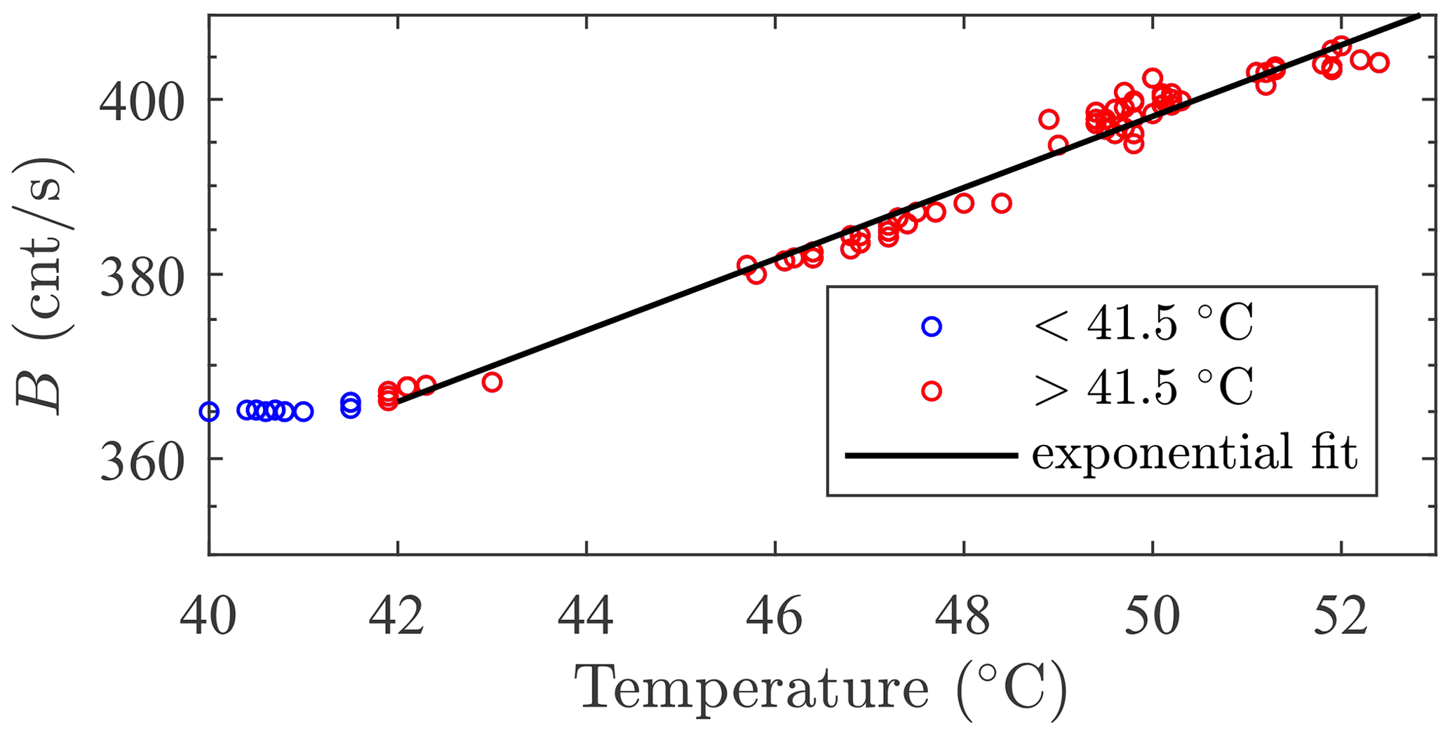
Figure 23 Variation in B due to dark-current increase with the instrument enclosure temperature above the 41.5 ^∘C (1040 nm channel). These measurements were acquired with the SPST05/M703 instrument during the Halifax campaign. The stabilized dark current is 365 cnt s⁻¹.

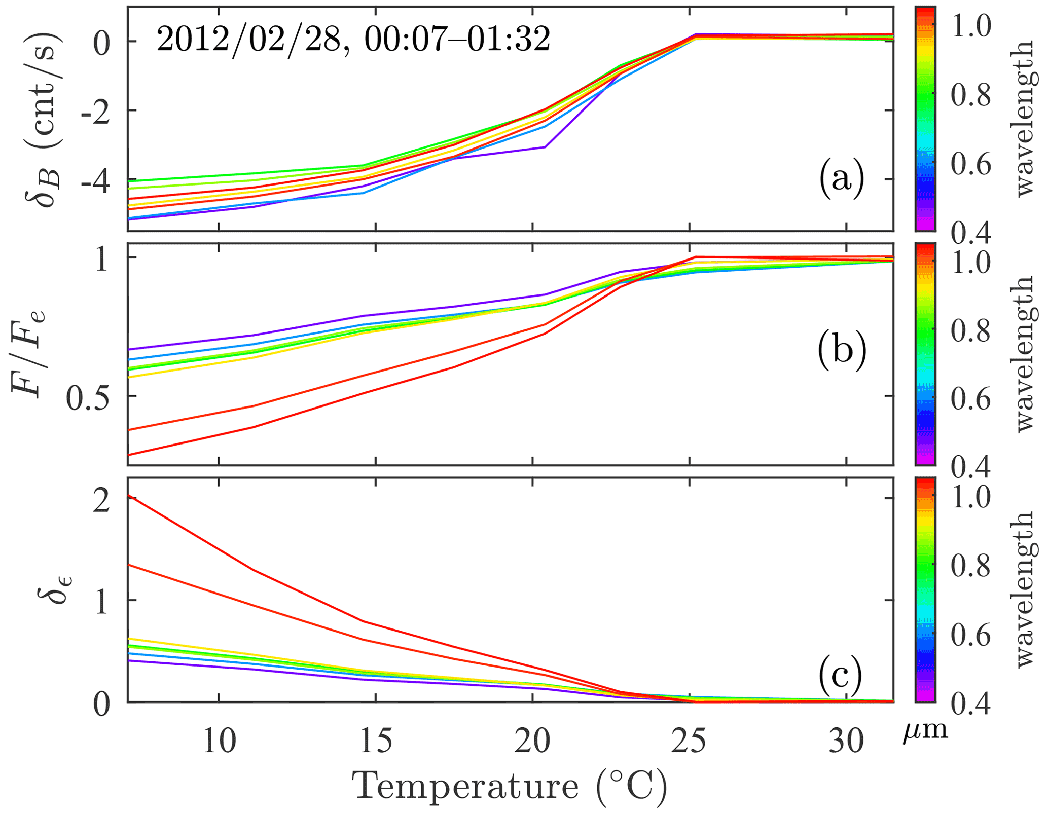
Figure 24 B variation (δ_B) due to dark-current decrease when the instrument enclosure temperature starts below the control range (a). Detector sensitivity as a function of temperature (b) and the corresponding observation error ${\mathit{\delta }}_{\mathit{ϵ}}=x{\mathit{\delta }}_{\mathit{\tau }}\simeq |F-F_{\mathrm{e}}|/F$ (c). The measurements shown in this figure were acquired with the SPST09/C11 at Eureka.

7.6 Throughput degradation

Even in the type of clean environment typically found at a mountain-top astronomical site, one can notice an optical throughput degradation due to dust deposition on telescope mirrors (Burki et al., 1995). Our starphotometers employ off-the-shelf (amateur) telescopes, with an optical corrector plate sealing off the optical train and being the main contact surface for any particle deposition. The formation of dew, frost, or the deposition of clear-sky snow crystals on that plate represents our greatest source of throughput degradation. Of particular concern is that humidity trapped inside the sealed telescope tube leads to dew or frost formation on the inside of the corrector plate (a degradation which cannot be easily removed by mechanical means). A dramatic frost-formation event that occurred during the Barrow campaign (in the absence of a dome or dew cap to protect the telescope) is illustrated in Fig. 25. The auto-calibrating Δ TSM (see Sect. 3.4.2) used to derive the green OD points shows little variation. This indicates that there was likely no aerosol and/or significant cloud OD variation during that period. However, the computed OD associated with the individual high and low stars varies strongly and is, based on our photographic evidence, attributable to frost formation on the plate. One should note that the ramping effects in the OD plot result from progressive frost formation and growth, after cleaning the instrument two separate times with a damp cloth. This operation did not apparently remove all of the frost (the OD values at the beginnings of the two ramps are higher than those acquired prior to the 09:00 UTC timestamp). One should also note that the low-star measurements (red data points) are less affected by the frost: this is because the throughput error, as represented by the OD variation from the baseline, is, as per Eq. (32), divided by a larger air mass.

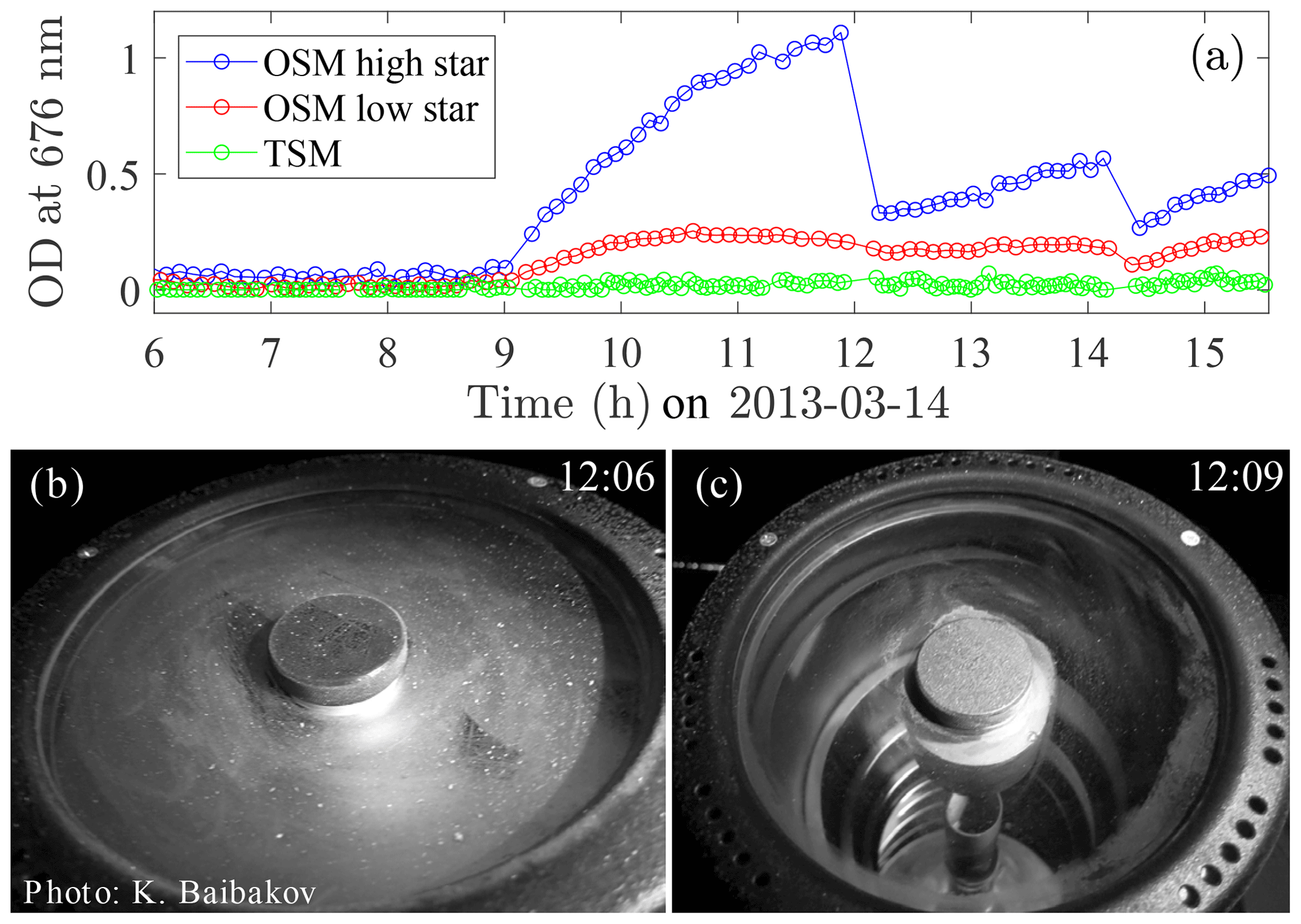
Figure 25 Extreme throughput degradation event caused by frost formation on the telescope corrector plate (Barrow campaign). The Δ TSM auto-calibrating mode effectively compensates, in real time, for any common-mode throughput degradation (attenuation increase) and, accordingly, remains largely unaffected by the frost (open green circles in panel a). In contrast, the OSM mode is very sensitive to the apparent attenuation of the high and low stars that constitute the TSM pair (respective blue and red open circles in panel a). The two rapid decreases in the OSM ODs correspond to cleaning events at 12:09 and 14:20 UTC. Panels (b) and (c) show the collector plate just prior to (12:06 UTC) and just after cleaning (12:09 UTC), respectively.

While one usually uses a dew cap to avoid fogging the optics at mid-latitudes, this technique cannot be used in the Arctic because the dew cap becomes a container for accumulating snow flakes and renders their mechanical removal difficult. One can usually sublimate the snow and frost from the external side of the corrector plate by closing the dome and increasing the dome temperature by few degrees. However, this does not represent a necessary real-time solution for preventing throughput degradation. In addition, it does not remove any internal telescope frost. Other experiments that have tackled this hurdle with limited success are described in Ivănescu et al. (2014). It initially seemed to be an impossible issue to solve, but a working solution was nevertheless identified, addressing both the frost and incoming crystals: a Kendrick Astro system using a controlled heating band wrapped around the telescope tube. This approach increases the temperature of the optics, particularly the corrector plate, by up to 10 ^∘C with respect to the environment. It was expected that this technique would increase the blurring of the starspots due to micro-turbulence near the telescope, but such an effect turned out to be negligible for our instruments.

8 Toward 1 % accuracy

A relative photometric error of 1 % in ${\mathit{\delta }}_F/F$ represents a magnitude error of δ_S≃0.01 and an observational error of ${\mathit{\delta }}_{\mathit{ϵ}}=x{\mathit{\delta }}_{\mathit{\tau }}=\mathrm{0.01}$. We seek to achieve the δ_ϵ<0.01 required accuracy goal, as discussed in Sect. 1, by mitigating the non-negligible systematic uncertainties identified in this paper.

8.1 Optimum channel selection

Some of the largest accuracy errors in starphotometry are, as explained in Sect. 4, due to contamination by stellar- and Earth-atmosphere (also called telluric) absorption lines, photometer spectral drift, bandwidth mismatch between the instrument and catalogue references, and airglow and aurora contamination, when present. These errors can be mitigated through a judicious channel wavelength selection. Avoiding high-frequency spectral influences is another reason for having narrow (<10 nm) channels. As remote sensing photometry is historically based on sunphotometry and is highly influenced by AERONET standards (the latest being Version 3; Giles et al., 2019), the World Meteorological Organization (WMO, 2016) recommendations for photometric-based aerosol observation includes AERONET (central) wavelengths. For consistency, one should endeavour to select at least a few AERONET bands. Sunphotometry is basically starphotometry based on a spectral-class-G2 star. Such stars have much weaker hydrogen absorption lines than the typical B and A stars of our catalogue. Therefore, our channel selection needs to consider the starphotometry reality, with its specific constraints: mainly to avoid hydrogen (H) lines and to ensure a star brightness (particularly challenging in the NIR region) much larger than the sky background. Furthermore, selecting more channels than the sunphotometers may help to compensate for typically larger starphotometer observation errors. The process of selecting more channels in starphotometry is facilitated by the fact that the number of channels employed by our (spectrometer-based) starphotometers is not constrained by the time-consuming constraints of an AERONET-type rotating filter wheel system. In what follows, we attempt to create an OD spectrum with the goal of identifying an optimal starphotometry band set under typical conditions. The method is constrained by an eventual fit to measured OD spectra.

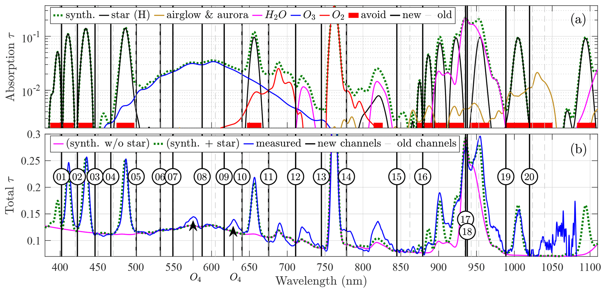
Figure 26 OD spectra of constituents that contaminate the retrieval of aerosol and cloud ODs in the visible and near-infrared. (a) Starphotometer channel selection (vertical black lines) obtained by avoiding contaminants, such as the stellar (Vega) absorption OD spectrum (black curve), OD errors associated with airglow and IBC2 aurora (gold curve) as well as O₂ (at least those parts of its red curve whose OD ≃0.01). The red bars delimit intervals where those contaminants are non-negligible (τ>0.007). The channel selection also includes strategically selected regions of H₂O and O₃ absorption that allow for the dynamic identification and characterization of their OD and, subsequently, their removal from the total OD spectrum. The cumulative contaminant optical depth yields the total synthetic curve (green dotted curve). (b) The synthetic curve (with an added aerosol scattering component) versus an OD spectrum (blue curve) retrieved from Vega measurements over Eureka (measured on 3 November 2019 at 14:01:02 UTC). The optimal fit shows generally good agreement except where the contaminant influence is misestimated. This is particularly true for O₄ absorption, which we realized, a posteriori, should have been included in the ensemble of contaminants. The numbers of the selected channels are superimposed for reference purposes.

The first step in our band selection process was to identify the spectral intervals free of stellar and aurora/airglow line contamination. To this end, we used the extraterrestrial (HST-measured) Vega spectrum (also shown in Sect. 4) at a 8.2 nm bandwidth. As Vega is a spectral-class-A0 star, its spectrum, which is strongly influenced by Balmer and Paschen H lines, is among the most affected by stellar absorption (Silva and Cornell, 1992). Inasmuch as the Vega spectrum can be considered the worst-case scenario, the systematic errors due to characteristic stellar absorption bands should be weaker for other stars. In order to obtain only the stellar absorption spectrum, we subtracted the continuum obtained by fitting the magnitude spectrum to data points not impacted by spectral absorption lines. The result, shown in Fig. 26a, was divided by 1.6 in order to simulate the air mass of an actual star. An IBC2 aurora OD error spectrum with respect to a V=2 star, along with an airglow 10 times larger than that in Fig. 15b, was employed to produce the gold “airglow & aurora” curve. The bottom red bars in Fig. 26a delineate the spectral intervals to be avoided, where the total of H lines and aurora contaminants are noticeable (>0.007). For realistic estimates of typical ODs for the most important telluric gaseous absorbers, we used laboratory-measured spectra. These included the O₂ results of Rothman et al. (2009) adjusted to typical Arctic levels (red curve), the H₂O results of Hill et al. (2013) adjusted to a typical wintertime precipitable water vapour value of 0.8 mm over Eureka (purple curve), and the O₃ results of Voigt et al. (2001) adjusted to 250 DU (blue curve). We neglected the NO₂ contribution, as the measurements of Lindenmaier et al. (2011) identified a maximum NO₂ column of 5×10¹⁵ molec. cm⁻² = 0.19 DU at Eureka in summertime, representing ${\mathit{\tau }}_{{\mathrm{NO}}_{\mathrm{2}}}=\mathrm{0.003}$ at λ=400 nm, whereas models estimate a much lower value in wintertime. The cumulative synthetic absorption spectrum of these component contributions is shown in dotted green in Fig. 26a. We employed the local minima of this curve as band placement indicators for which errors in ascribing values to the ensemble of absorption contributions (which one must inevitably do to extract an aerosol or cloud OD) would be minimized. A set of 20 new channels (solid black vertical lines) was identified as a potential replacement for the old set of 17 channels (dashed grey vertical lines) currently employed in our starphotometers (this also represents approximately 3 times the number of channels employed in the AERONET instruments). The dotted green curve in Fig. 26b shows the same dotted green cumulative spectrum as in Fig. 26a to which aerosol scattering has been added. The aerosol scattering OD was assumed to vary as per the classical Ångström expression of bλ^−a, while b was incrementally perturbed until it matched an actual OD Vega spectrum (blue curve) measured at Eureka (a typical value of 1.3 was assumed for a). For reference, the same spectrum but without the stellar components is represented in purple. The position of the 20 new channels are duplicated in Fig. 26a in order to better appreciate the final total OD context for those positions.

The selection procedure identifies as many channels as possible, constrained by the avoidance of any absorption line contamination. The ultimate goal is the characterization of the low-frequency (slowly varying) aerosol and cloud scattering spectrum. As there are large spectral intervals where that is not possible (mainly across the O₃, O₂, and H₂O absorption bands), one also needs to include channels that independently facilitate the extraction of O₃ and H₂O column abundances (at least two channels per band, as they are noisier due to the strong absorption). The newly identified central channel wavelengths as well as their application and their reason for selection are summarized in Table 2.

Table 2 Specifications for the 20 starphotometry channels chosen according to the absorption feature avoidance process outlined in the text (see the text for details on the reason(s) for selection).

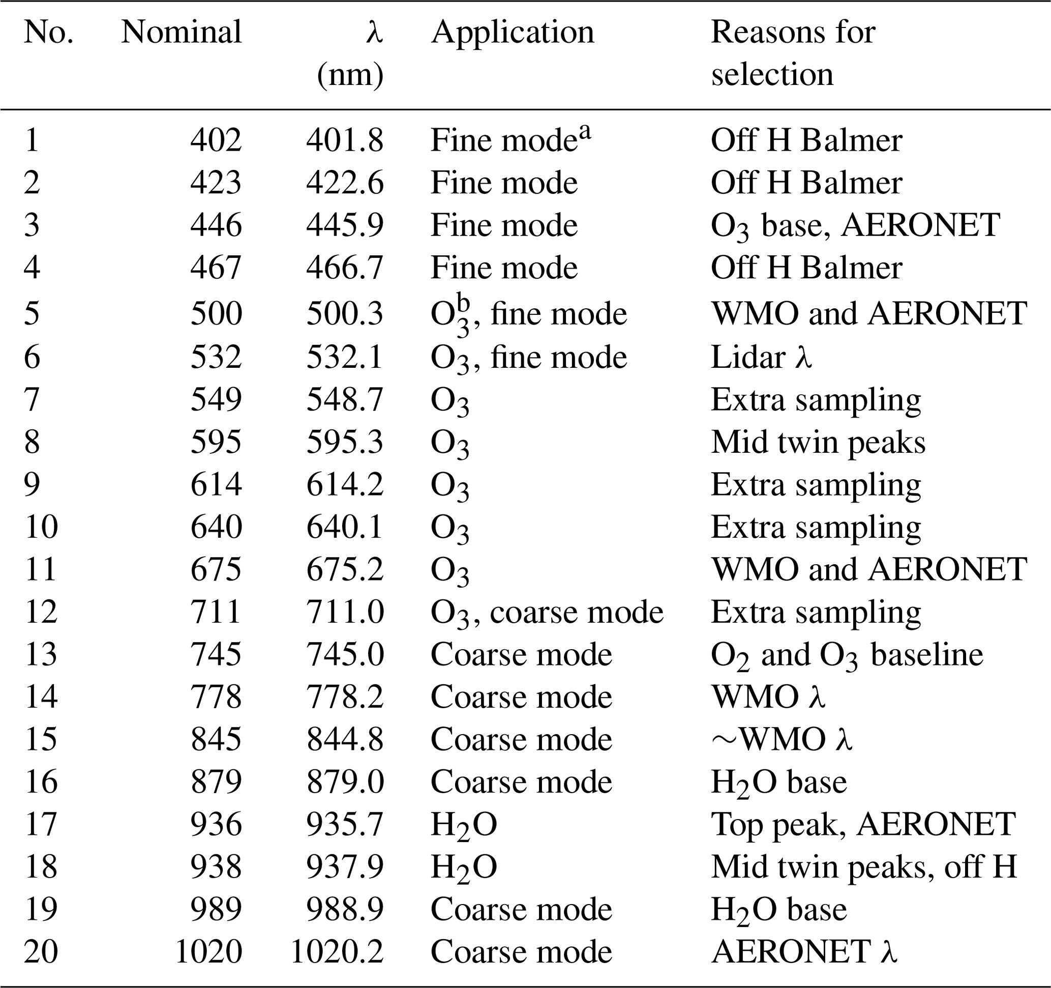
^a Spectral region that is more sensitive to the characterization of fine-mode (FM) aerosol properties such as FM aerosol OD. The total aerosol OD (FM OD and coarse mode OD) will be sensitive to the presence of FM aerosols. ^b O₃ absorption is strong enough to provide a retrieval of O₃ columnar abundance and, thus, O₃ OD from a spectrally dependent matching type of total OD retrieval and, accordingly, to correct (eliminate) the O₃ OD from the total OD for all O₃-affected channels.

The justifications for the 20 selected channels (sequentially ordered as per Table 2) are given below:

1. Channel 1 was chosen in order to avoid or minimize H contamination. It also better constrains the UV/blue trend of the fine-mode aerosol spectrum.

2. Channel 2 was chosen in order to avoid or minimize H contamination. This is the optimum λ identified in Sect. 4.

3. Channel 3 was chosen to avoid a H line and the 440 nm emission line identified in Sect. 6.4. This band is near the 440 nm AERONET channel and can be used as the lower-bound baseline for isolating the O₃ OD band.

4. Channel 4 was also chosen to avoid a H line. Both channels 3 and 4 are moved slightly left with respect to the current (old) channels in order to increase their sensitivity to aerosols.

5. Channel 5 is a WMO recommendation and an AERONET channel.

6. Channel 6 is a lidar standard channel.

7. Channel 7 is a good channel for sampling the ozone profile shape while avoiding the 557.7 nm aurora and airglow peak.

8. Channel 8 is a strong O₃ OD channel that lies between double-ozone peaks. It is one of three bands sensitive to O₃ abundance (and, thus, O₃ retrieval), and it avoids side bands of O₄ contamination and any possible twilight contamination by 589 nm sodium flashes (Chamberlain, 1995). We note a shortcoming in our synthetic curve around 590 and 640 nm – the absence of O₄ absorption features (see Wagner et al., 2002, for information on O₄ absorption and Michalsky et al., 1999, for O₄ spectrum analysis).

9. Channel 9 is a strong O₃ OD channel that also avoids an O₄ line. It has the same mandate as band 8 (sensitive to O₃ abundance).

10. Channel 10 was chosen in order to avoid O₄ and H lines. This band has a useful spectral placement for characterizing the O₃ profile shape, but it requires correction for O₂ contamination (note the marginally significant strength of the O₂ OD in Fig. 26a).

11. Channel 11 is a WMO recommendation and an AERONET channel, and it requires correction for O₂ contamination.

12. Channel 12 is a new channel that fills what, up to this point, has been a large spectral gap characteristic of our instruments. It was also chosen in order to avoid a nearby H₂O line, and it requires correction for O₂ contamination.

13. Channel 13 was chosen in order to avoid the water vapour line at ∼840 nm and the strongest O₂ line at ∼761 nm. This channel can be used as a lower- and upper-bound baseline for the O₂ and O₃ absorption profiles, respectively.

14. Channel 14 is a WMO recommendation. It was also chosen in order to avoid the 840 nm H₂O line and the 761 nm O₂ line, and it requires correction for O₂ contamination.

15. Channel 15 was chosen in order to avoid the 840 nm H₂O line. It requires correction for O₂ contamination. This channel is near the WMO 862 nm recommendation, but the latter may be affected by aurora OD errors.

16. Channel 16 was chosen in order to avoid H₂O and H lines. This channel is meant to serve as a lower-bound baseline for the broad H₂O absorption profile that starts around 890 nm.

17. Channel 17 captures maximum H₂O absorption (free from H contamination) and is used for the retrieval of H₂O abundance. The choice of a maximum also minimizes the influence of the line-shape variation as a function of water vapour abundance (Volz, 1969). This is practically the same as the main (935 nm) AERONET channel employed for precipitable water vapour (PWV) retrieval.

18. Channel 18 is the second H₂O channel and was chosen to improve measurement precision under low-starlight-flux conditions due to strong H₂O absorption and generally low starlight flux in the NIR region.

19. Channel 19 was chosen in order to avoid H₂O and H lines. This channel is meant to serve as a lower-bound baseline for the broad H₂O absorption profile that ends around 990 nm. It also avoids the region of the strongest aurora- and airglow-induced OD errors.

20. Channel 20 was chosen because it is the largest NIR wavelength that still provides accurate measurements while avoiding H lines. Even if this channel is relatively sensitive to airglow emissions, it can be considered reasonably reliable for V=0–1 BA-class stars or bright (and colder) F-class stars, such as Procyon, whose NIR flux is relatively strong.

The major changes and improvements with respect to the original channel set are as follows: a new 402 nm channel to better estimate the UV attenuation due to fine-mode aerosols; the 432 nm channel is optimized for minimal contamination; the ozone absorption profile is oversampled to allow better removal in post-processing; the 953 nm H₂O channel was excluded (see the peak on the right side of Fig. 26a, on top of the H₂O band), as it is likely influenced by a H Paschen line; the H₂O baseline is better estimated with more strategically selected baseline channels (closer to the limits of significant absorption); the original (persistently noisy) 1040 nm channel was excluded (the high-frequency variations seen in the retrieved ODs above approximately 1030 nm in Fig. 26b are a symptom of the noisy nature of signals in that region of the NIR). In order to avoid NIR airglow, one needs only acquire data at wavelengths above 1050 nm; however, this results in a weaker star flux and the above-mentioned weak signal-to-noise ratio. Finally, we remind the reader that our channel selection process is optimized for the peculiarities of our starphotometer. Signal-to-noise considerations aside, the spectral bandwidth is one of those peculiarities: different bandwidths may require slightly different channels.

8.2 Starphotometry recommendations

Table 3 provides a summary of the accuracy error sources that we investigated: the 20 starphotometry channels defined in the previous section are recommended, at least in part, to minimize their impact. In general, these channels are dedicated to the extraction of aerosol and/or cloud ODs as well as the strong O₃ and H₂O molecular absorption ODs (either as corrections to achieve estimates of aerosol and cloud ODs or as remote sensing targets on their own merit). Details on the extraction procedures are given in King and Byrne (1976), Michalsky et al. (1995), Taha and Box (1999), Xia and Wang (2001), and Box and Taha (2001).

Table 3 Summary of accuracy error sources that would propagate in the τ retrieval, their typical values, and estimates of their upper limits. Water vapour channels were not considered.

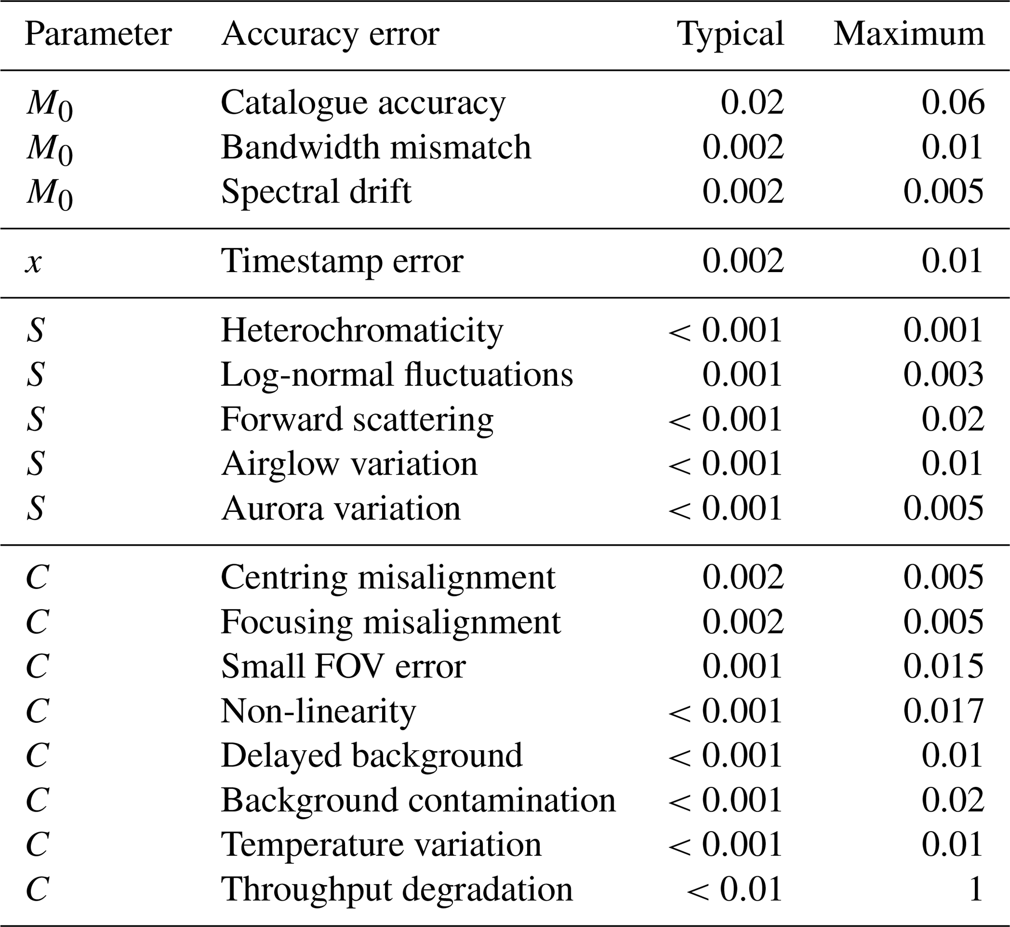
An important source of OD error is related to the accuracy of the spectrophotometric catalogue. In the case of the Pulkovo catalogue, we identified a particularly large bias in the UV and 900–1000 nm regions (see the text associated with Fig. 4) that could distort the retrieved aerosol spectrum. That bias aside, the errors in the individual star spectra are particularly prohibitive in terms of achieving the required accuracy. It is strongly recommended that a new and improved bright-star catalogue should be made, preferably with magnitude measurements acquired by a space-based instrument, to avoid the incertitude related to telluric absorption contributions. As discussed in Sect. 4, the requirements for such a catalogue are a 1 nm bandwidth and <1 nm (preferably 1 Å) spectral resolution, with less than 0.01 differential magnitude variation across the measured spectrum. In the mean time, we continue to use the Pulkovo catalogue but with its 8.2 nm bandwidth version, which improves the bandwidth match with our instruments and offers a wider bright-star diversity than what is currently provided by HST. Alternatively, if the starphotometer is a spectrometer-based instrument, as is our starphotometer, one can generate such a catalogue from direct high-resolution observations (all spectrometer channels) at a high-altitude site. Such a catalogue would perfectly match the instrument bandwidth. We recommend that future starphotometer bandwidths be confined to less than 10 nm: this is an easily attainable standard that ensures negligible heterochromatic errors (δ_τ<0.001). The employment of all of our 1000 spectrometer channels for spectral drift corrections (not only the proposed 20 operational channels) ensures that any high-resolution stellar features can be properly avoided. Observations and calibration should be preferentially performed with a B0–B3 (early-type B) star or with A7–A9 (late-type A) and F stars in order to avoid the incertitude related to the strong stellar absorption lines. Furthermore, annual spectral calibration is advisable in the face of the drift results in Fig. 8. Alternatively, measurements of a high-resolution spectrum of a particularly bright star of near-A0 type (notably Vega) could be carried out every few months. Its deep $H_{\mathit{\alpha },\mathit{\beta },\mathit{\gamma }}$ Balmer lines will serve (along with the Earth's O₂ and H₂O lines) as a reference for spectral calibration in post-processing. One particular concern at mid-latitude locations is that NO₂ may be several times larger (Cede et al., 2006) than at Eureka (i.e. up to 0.03 OD at 400 nm or 0.01 OD at 500 nm), and its absorption will no longer be negligible. As NO₂ absorption is impossible to discriminate from aerosol spectrum, it has to be assessed from independent sources.

Retrievals in the presence of rapid temporal variations of sky brightness (a measurement which must accompany every star measurement) must be corrected by interpolating from pre- and post-contaminated sky brightness measurements to the time of the star measurement. Signals greater than the threshold for the onset of non-linearity (8000 cnt s⁻¹ in the case of our starphotometer) should be discarded (Sect. 7.2). Under such bright sky conditions, one may expect OD errors >0.017, unless interpolating the sky brightness to the timestamps of star measurements. One should be aware that, with an increase in sky brightness, the blue part of the spectrum saturates first, leading to a distorted aerosol spectrum retrieval.

Air mass accuracy should be ensured by the use of a GPS time server. OD errors associated with air mass uncertainties can also be reduced at a high-altitude site, while they remain sensitive to time errors on low stars, i.e. at large x (see Fig. 12). The internal instrument temperature should be monitored, as the temperature controller may eventually fail (e.g. at the very low environmental temperatures found in the Arctic). In particular, the user needs to wait for the system to warm up to its stabilized range, as low temperatures have a larger error impact (see Sect. 7.5).

The stability of the throughput has fundamental impact on the calibration process. Due to the excessively small FOV of the SPST09/C11 configuration (36.9 arcsec), the optical alignment proved to be critical to ensuring stable throughput. As demonstrated in the discussion surrounding Fig. 18, the centring tolerance error should not exceed 4 arcsec for this instrument at Eureka (two CCD bins). The focusing error of SPST09/C11 should always be within one step adjustment step (confusion circle variation of ∼10 arcsec per step, as per the legend of Fig. 17). This means, for example, that the focus must be adjusted by one step for each 10 ^∘C change in outside temperature.

Turbulence analysis using starspot imaging revealed another large source of throughput degradation, which is acerbated at Arctic sea level sites: possible vignetting of starspots at large air masses. This problem was ascribed to the small SPST09/C11 FOV in the context of the excessively larger seeing at Eureka. The worst-case (m=10) scenario of the red curve in Fig. 2 (for which the starspot is ω≃19 arcsec) can be accommodated by a FOV of $\mathrm{2.3}\cdot \mathit{\omega }\simeq \mathrm{45}$ arcsec (see Appendix C for details). In the light of the forward-scattering error analysis, one should not increase it beyond ∼47 arcsec (roughly where the mean of the most demanding case in Fig. 14, the “120 µm (ASC) ice cloud” case, crosses the 0.01 value of the ${\mathit{\delta }}_{\mathit{\tau }}/\mathit{\tau }$ axis). This FOV limitation also ensures accurate measurements (sub-1 % errors associated with the brightness contamination cases in Figs. 15 and 16) during faint aurora (IBC2) events (or their illumination equivalence of thin moonlit cirrus clouds) for even weak (V=3) stars (with the NIR exception in Fig. 16, where a bright V=0 star, such as Vega, is needed to achieve the 1 % threshold). Therefore, a 45 arcsec FOV, which would be obtained with a 0.61 mm diaphragm in the C11 case, appears to be good compromise between the conflicting requirements of maximizing the FOV to accommodate all starspot sizes (red curve in Fig. 2) and limiting the FOV to minimize the largest forward-scattering errors (blue curves in Fig. 14). The small FOVs employed in starphotometry ensure that this technique is significantly less dependent on the intrinsic and artificial OD reduction induced by scattering into the FOV by optically thin clouds. This singular capability of starphotometry renders it rather unique in extinction-based photometry inasmuch as sun- and moon-based techniques require (or at least traditionally use) much larger FOVs and accordingly suffer from much larger FOV scattering contamination.

We demonstrated (Sect. 7.1) that observations at air masses higher than ∼5 should not be made with the C11 because of the influence of vignetting. Calibration may, nevertheless, be performed beyond this air mass limit, as long the S values still show a linear dependence on x. This may happen under weaker air turbulence conditions than those in Fig. 2. Throughput degradation due to frost/dew or ice crystal deposition on the telescope was a long-standing problem for our Eureka starphotometer (with critical accuracy implications). The use of the Kendrick system (or similar heating bands), together with a small wind shield, proved to be a reliable solution which would be appropriate for most of Arctic observation sites. If all these recommendations are followed, one may aspire to achieve a reduction in each zenith OD error component to well below 0.01 and the total zenith OD error to ≲0.01 (i.e. the stated 1 % photometric accuracy). Even if these goals are, in certain cases, still under development, any progress that substantially approaches the goal of 0.01 total zenith OD error would represent a significant advance in starphotometry reliability.

9 Conclusions

With the ultimate goal of improving starphotometry accuracy, we analysed a large variety of sources that could induce systematic (absolute) errors and classified them by their impact on each parameter involved in the OD retrieval. The contamination from stellar and telluric gas absorption lines may induce large OD errors. One example of such contamination, the O₄ absorption lines, can affect O₃ estimation and removal with attendant distortion of the aerosol OD spectrum. Such errors are, nevertheless, mitigated with proper channel allocation: this was demonstrated using synthetic and measured OD spectra to extract a set of 20 optimal channels. In order to further minimize the absorption-line-induced OD errors (stronger hydrogen lines tend to spill over into different bands), one may favour the starphotometry observations using early-type B as well as late-type A and F spectral class stars, which have weaker hydrogen absorption lines. Therefore, we may particularly prefer them for calibration purposes.

Inaccuracies in the current exoatmospheric photometric catalogue can be partly addressed in the Δ TSM observation mode (where the catalogue bias is cancelled out) or by circumventing the catalogue with lengthy calibrations involving each star that one wishes to employ as an extinction target (calibrations using Langley calibrations at a high-altitude site, for example). Given such restrictive options, the community is strongly encouraged to prioritize the development of a new spectrophotometric catalogue with improved accuracy, supported by magnitude variability characterization. This will increase confidence in the accuracy of a star-independent calibration and will render that approach more operational and reliable.

Problems related to the instrument instability (including spectral drift and starspot vignetting) were identified, and appropriate observation strategies and design improvements were proposed. Beyond the current accuracy assessment study, we will pursue starphotometry reliability improvement by also characterizing the non-systematic, random errors, as well as those related to C-value retrievals through Langley plot calibration. A sky brightness model to estimate the background of moonlit and twilight-lit clouds is in development. A new exoatmospheric photometric catalogue based on GOMOS satellite photometry is also envisioned. In order to validate the proposed improvements, one should participate in observation campaigns and compare the observations with other co-located instruments. The Cimel moonphotometer and the profiling backscatter lidar at our Eureka site are co-located instruments that already provide support of this nature.

As an original by-product of this study, we developed a semi-empirical expression for estimating the seeing (starspot blurring) profile from radiosondes measurements.

Appendix A: The Canadian starphotometry program

Our group at the Université de Sherbrooke has been performing starphotometry observations of aerosols and optically thin clouds in Canada and elsewhere since 2007. There have been a total of three Canadian sites in our small starphotometer network: the high-latitude site at Eureka (Nunavut) and mid-latitude sites at Sherbrooke, Québec, and Egbert (Ontario). Currently the network has been reduced to the Eureka and Sherbrooke sites. Additionally, campaign-based observations took place in Halifax (NS), Barrow (Alaska, USA), and Izaña (Canary Islands, Spain).

A1 The instruments

Our starphotometers were built by Dr. Schulz & Partner GmbH, a German company that has now ceased operations. A total of nine instruments, with serial numbers from SPST01 to SPST09, were produced. The first three were initial development versions (now decommissioned), and the remaining six are still in operation. Three of these are German-owned instruments: SPST04 is still at the manufacturer, and SPST07 and SPST08 are being operated by the Deutscher Wetterdienst (DWD) Meteorological Observatory of Lindenberg (Germany) and by the Alfred Wegener Institute (AWI) at Ny-Ålesund (Svalbard), respectively. The other three are Canadian-owned instruments: SPST05 is at the Université de Sherbrooke; SPST06, formerly at the Egbert Environment and Climate Change Canada (ECCC) site, has been decommissioned; and SPST09 is at the Eureka OPAL site (Ivănescu et al., 2014). The SPST04 to SPST07 instruments are all the same version, whereas the two most recent versions, SPST08 and SPST09, are upgrades. The common detection device employed for all those versions is the QE65000 scientific-grade spectrometer from Ocean Optics. The QE65000 is based on a Hamamatsu S7031-1006 CCD sensor (1044 pixels × 64 pixels). We use two different telescopes, both with an $f_{\mathit{\#}}=f/D=\mathrm{10}$ focal ratio, where f is the focal length and D the diameter.

The telescope “plate scale” P_s on the focal plane can be computed (Carroll and Ostlie, 2007) with

$$P_{\mathrm{s}}=k_c/f=k_c/(D\cdot f_{\mathit{\#}}),$$

where P_s is in units of arcseconds per millimetre (arcsec mm⁻¹), $k_c=\mathrm{3600}\cdot \mathrm{360}/\left(\mathrm{2}\mathit{\pi }\right)=\mathrm{206264.8}$ arcsec rad⁻¹ is a radian to arcsecond conversion factor, and f and D are in millimetres (mm). The version to version improvements mainly concern the robustness of the instrument. However, the throughput of the SPST09 instrument is a factor of 3.2 better than the previous version due to the use of an 11 in. diameter (279.4 mm) Celestron C11 Schmidt-Cassegrain telescope with StarBright XLT coating and a 98 mm diameter (secondary mirror) central obstruction (11.5 % of the primary mirror surface). The previous models used a 7 in. (177.8 mm) Alter M703 Maksutov-Cassegrain telescope with a 32 % (secondary mirror) central obstruction (100 mm diameter). The internal optics of the SPST09 are currently coated with (Melles Griot) Extended HEBBAR™ coating. By comparison, all other starphotometer versions have custom coatings with about a 3 magnitude throughput loss around 500 nm but about a 1 magnitude gain in the infrared. All versions perform measurements simultaneously across 1000 channels along the 1044 pixels of the CCD: only 17 (multi-pixel) bands were selected by the manufacturer as a standard for regular operation (see Table 1). Near-star, night sky radiance for background subtraction from the stellar signal is measured by pointing the photometer about 8 arcmin (arc minutes) off-target. The star-acquisition procedure is based on star centring by two auxiliary SBIG ST-402ME-C2 CCD cameras. A square 504 pixels×504 pixels (px) subframe of the available 510×765 px CCD frame is employed. For speed and sensitivity, the acquisition mode uses 3×3 bins of 9 µm square pixels (i.e. 27 µm ×27 µm bins). The initial wide-field centring uses a 67 mm diameter refractive auxiliary telescope with a fast f_#=4 focal ratio. Its P_s=12.65 arcmin mm⁻¹ plate scale provides a 57.4 arcmin field of view (FOV) on its camera, with 20.5 arcsec per bin (arcseconds per three-pixel bin). The subsequent centring is done at high angular resolution using the main telescope. The P_s=73.7 arcsec mm⁻¹ plate scale of the C11 telescope provides a 5.6 arcmin FOV, at 2 arcsec per bin. The P_s=114.6 arcsec mm⁻¹ plate scale of the M703 telescope provides a 8.3 arcmin FOV, at 3 arcsec per bin. Based on the Nyquist–Shannon sampling theorem (Shannon, 1948), one can track starspots at the maximum precision of 1 bin if one has at least 1 bin per standard deviation of the starspot (Robertson, 2017), or 2.355 bins per full width at half maximum (FWHM). This would be the case for starspot FWHMs larger than 4.7 arcsec for the C11 and 7.1 arcsec for the M703. This condition is easily satisfied for the C11, but it is only satisfied for m≳2.5 in the case of the M703 (see Fig. 2). To avoid contamination from off-target objects, one limits the measured FOV with a 0.5 mm diameter diaphragm at the telescope focus. This means, based on the corresponding plate scale, that the spectrometer (i.e. the actual detector) FOV is 36.9 arcsec for C11 and 57.3 arcsec for M703. The starlight is then refocused on a 400 µm diameter optical fibre that feeds the QE65000 grating spectrometer through a 200 µm wide slit. The diffraction profile, on the spectrometer's 1044 pixel long CCD, covers several (24.6 µm ×24.6 µm) pixels at 0.7 nm bandwidth per pixel. In order to improve the measurement accuracy, one averages five pixels (±2 around the central pixel). The convolution of the slit function with the averaged pixels leads to a profile with a FWHM ≃8.2 nm, or 12 pixels (the bandwidth reported in Sect. 4). Assuming Gaussian-shaped bands, each channel suffers >1 % contamination from blur within 10 nm of its centre. The typical starphotometer measurement implies simultaneously averaging several (usually three or five) 6 s exposures, in all channels. Other technical parameters are listed in Table 1. All instruments are protected by astronomical domes. There are 12 ft (3.66 m) and 7 ft (2.13 m) diameter Astro Haven domes at Sherbrooke and Egbert, respectively, while Eureka boasts a 10 m diameter dome built especially for Arctic conditions by the Baader Planetarium in Germany (Fig. 1). The tracking system (the telescope mount) at Sherbrooke and Egbert is the Losmandy G-11 German equatorial mount. An AZA-2000 Dobsonian alt-azimuth mount, especially built for the Arctic by the 10Micron (Italy), is employed at Eureka.

A2 Observation sites

The Sherbrooke, Quebec, site is located within the Université de Sherbrooke campus, on the roof of the SIRENE (Site Interdisciplinaire de REcherche en ENvironnement Extérieur) measurement station (45.374^∘ N, 71.923^∘ W; ground elevation + instrument height of 308 + 6 m a.s.l. The Egbert, Ontario, site is at the ECCC Centre for Atmospheric Research Experiments (44.232^∘ N, 79.781^∘ W; 251 + 6 m a.s.l.), located 65 km north of Toronto, Ontario.

The Eureka, Nunavut, site (79.991^∘ N, 85.939^∘ W; 10 + 2 m a.s.l.), which is part of the Zero Altitude PEARL Auxiliary Laboratory (0PAL) site near the ECCC Eureka Weather Station, is our most prolific data provider. Polar night data, from roughly late September to late March, were acquired from 2008 to 2010 using the SPST05/M703 instrument. The upgraded SPST09/C11 collected data for about 2 months during each observation seasons until 2014 with a gap in 2012–2013 (Ivănescu et al., 2014). After overcoming several technical difficulties, the acquisition period was extended to 3–4 months from 2015 onwards.

The Halifax site was on the roof of the Sir James Dunn Building (44.638^∘ N, 63.593^∘ W; 45 + 6 m a.s.l.), at Dalhousie University. A total of 2 weeks of data were acquired with SPST05/M703 during the July 2011 BORTAS (BOReal forest fires on Tropospheric oxidants over the Atlantic using Aircraft and Satellites) campaign. Outside of Canada, we performed SPST06/M703 observations for about a week in October 2008 at the Izaña Atmospheric Research Center in Tenerife, Canary Islands, Spain (28.309^∘ N, 16.499^∘ W; 2390 + 1 m a.s.l.). In March 2013, we carried out a SPST05/M703 field campaign at the Barrow, Alaska Observatory (71.323^∘ N, 156.611^∘ W; 11 + 2 m a.s.l.).

Appendix B: Star dataset

Our 20-star selection from the dataset of Northern Hemisphere bright stars is presented in Table B1. These stars were selected for their stability (with the requirement that declination (DE) ≳ −23.5^∘ to account for Earth axis inclination): the 13 positive-DE stars are usually present in the Arctic sky. One can always form a (“high”, “low”) pair from those 13 stars and, thus, have recourse to the TSM mode.

Table B1 Star selection from the Northern Hemisphere bright stars. These stars are usually referred to by their Harvard Revised (HR) Bright Star photometry catalogue (Pickering, 1908). Their HD (Henry Draper catalogue; Cannon and Pickering, 1918) and HIP (Hipparcos catalogue; van Leeuwen et al., 1997) codes are also listed in order to facilitate their identification. The subsequent columns show their affiliated rank (Greek letter) and constellation, common name, right ascension (RA), declination (DE) coordinates at epoch 2000, and visual magnitude (V). GCVS and Hipparcos peak-to-peak magnitude variations (ΔV and ΔHp, respectively) are indicators of star stability. The next column shows the spectral class (Sp) of the star (including its 0–9 numerical subclass) and its luminosity class (Lum). The last column is specific to the Arctic; it indicates the TSM role of each Arctic star (“high” or “low”), as described in Sect. 3.4.2.

^a From General Catalog of Variable Stars, version GCVS 5.1 (Samus et al., 2017). ^b From Hipparcos Main Catalog (van Leeuwen et al., 1997).

The General Catalog of Variable Stars (GCVS; the source of the ΔV parameter) is built on old observations dating as far back as 1949, while the Hipparcos catalogue (the source of the ΔHp parameter) has a photometric resolution magnitude limit of 0.01 but only intermittently monitors a given star. While ΔHp ≤0.01 for only a few stars in Table B1, there are 24 such V<3 stars in the Pulkovo catalogue. Given the uncertainty in star variability, as evidenced by discrepancies between the ΔV and ΔHp columns of Table B1, a proposal for a new Table B1 dataset should wait for a more reliable future photometric catalogue.

The similar spectral class constraint on pairs of Δ TSM stars (Sect. 4) indicates that the Table B1 pairings should be the (HR 7001, HR 7557) of A class as well as the (HR 1791, HR 1790) and (HR 5191, HR 3982) of B class. These pairs have similar right ascension (RA) values (meaning that they are fairly close in azimuth) and, together, cover the entire 24 h period (while ensuring air masses <6 for low stars). We note that the spectral subclasses differ substantially for all three pairs (i.e. the 0–9 class suffix): however, if we loosen the RA criterion, the alternate (HR 5191, HR 1790) pair may be of sufficiently similar subclass.

Appendix C: FOV constraints

The long-exposure PSF is characterized by a FWHM≃ω and a standard deviation $\mathit{\sigma }=\mathit{\omega }/\mathrm{2.355}$. A large part of the PSF is due to random starspot movements, called jitter (θ). The fact that the short-exposure movement is tracked dynamically by the starphotometer means that the low-frequency jitter (θ_L) is largely reduced and, thus, will not contribute to the starspot fed into the photometer. We estimate ${\mathit{\sigma }}_{{\mathit{\theta }}_{\mathrm{L}}}^{\mathrm{2}}$ by integrating the jitter power spectrum, from zero up to the tracking bandwidth (i.e. half of the low-frequency value given in Eq. 15 of Glindemann, 1997). When the tracking bandwidth tends to the sampling frequency ($\mathrm{1}/t$), the missing jitter contribution to ω is (ibid)

$$\begin{array}{}\text{(C1)}& {\mathit{\omega }}_{{\mathit{\theta }}_{\mathrm{L}}}=\mathrm{2.355}\cdot {\mathit{\sigma }}_{{\mathit{\theta }}_{\mathrm{L}}}=\mathrm{0.917}{\left({\displaystyle \frac{r_{\mathrm{0}}}{vt}}\right)}^{\mathrm{1}/\mathrm{6}}\mathit{\omega }\end{array}$$

where this equation and all equations in this Appendix are homogeneous as a function of angle (i.e. the use of a non-standard angular argument, such as arcseconds, scales coherently on both sides of homogeneous equations). The turbulence length parameter was found to be r₀≃0.01 m for Eureka (Sect. 2), and v≃10 m s⁻¹ is the typical effective wind speed. The operational starphotometer exposure value of t=6 s yields

$$\begin{array}{}\text{(C2)}& {\mathit{\omega }}_{{\mathit{\theta }}_{\mathrm{L}}}=\mathrm{0.215}\cdot \mathit{\omega }.\end{array}$$

The FWHM of the t=6 (starphotometer) short-exposure spot in a Kolmogorov turbulence is ${\mathit{\omega }}_{\mathrm{s}}=({\mathit{\omega }}^{\mathrm{5}/\mathrm{3}}-{\mathit{\omega }}_{{\mathit{\theta }}_{\mathrm{L}}}^{\mathrm{5}/\mathrm{3}}{)}^{\mathrm{3}/\mathrm{5}}\simeq \mathrm{0.95}\cdot \mathit{\omega }$ or more, depending on the performance of the tracking system. This means that the tracking basically applies a negligible correction to ω. Averages of the Fig. 2 (ω_s) points for a given value of m indicate a ratio relative to ω that is somewhat smaller than the 0.95 implied above. In effect, the preparation of Fig. 2 necessitated short exposure time reductions from the 6 s operational standard in order to circumvent problems such as signal saturation: this figure is more realistic in terms of providing a cross section of short exposure times that might be used by starphotometers in general.

Based on Eq. (77) from Tyler (1994) and Eq. (5) from Racine (1996), the standard deviation of the total jitter σ_θ is

$$\begin{array}{}\text{(C3)}& {\mathit{\sigma }}_{\mathit{\theta }}=\mathrm{0.42}\cdot (\mathit{\lambda }/D{)}^{\mathrm{1}/\mathrm{6}}\cdot {\mathit{\omega }}^{\mathrm{5}/\mathrm{6}}.\end{array}$$

For our instruments and telescopes, $(\mathit{\lambda }/D{)}^{\mathrm{1}/\mathrm{6}}\simeq \mathrm{1}$ arcsec. One can show that, for 5 arcsec $<\mathit{\omega }<\mathrm{15}$ arcsec (i.e. the ω range at m<5 in Fig. 2), one can approximate ${\mathit{\omega }}^{\mathrm{5}/\mathrm{6}}\simeq \mathrm{0.7}\cdot \mathit{\omega }$ and recast Eq. (C3) as

$$\begin{array}{}\text{(C4)}& {\mathit{\sigma }}_{\mathit{\theta }}\simeq \mathrm{0.4}\cdot {\mathit{\omega }}^{\mathrm{5}/\mathrm{6}}\simeq \mathrm{0.3}\cdot \mathit{\omega }.\end{array}$$

Using Eq. (C2), one retrieves the high-frequency component of the jitter as ${\mathit{\sigma }}_{{\mathit{\theta }}_H}=({\mathit{\sigma }}_{\mathit{\theta }}^{\mathrm{2}}-{\mathit{\sigma }}_{{\mathit{\theta }}_{\mathrm{L}}}^{\mathrm{2}}{)}^{\mathrm{1}/\mathrm{2}}\simeq \mathrm{0.21}\cdot \mathit{\omega }$. This represents an ω-dependent estimation of the starspot displacement between the starphotometer measurements. A centring tolerance of ${\mathit{\delta }}_{\mathrm{c}}={\mathit{\sigma }}_{{\mathit{\theta }}_H}$, specified in the star-centring process (for an assumed Gaussian probability distribution of the random jitter), ensures that about two-thirds of the subsequent short-exposure measurements will still be centred (see Fig. C1 for a schematic of starspot positions and their defining parameters). The (m=5) long-exposure ω values at Eureka and Sherbrooke of 14.7 and 8.9 arcsec, respectively (Fig. 2), imply a (${\mathit{\delta }}_{\mathrm{c}}\simeq \mathrm{0.21}\cdot \mathit{\omega }=\mathrm{0.2}\cdot {\mathit{\omega }}_{\mathrm{s}}$) centring tolerance of 3.1 and 1.9 arcsec, or roughly two and one pixels, respectively. This is consistent with the $\mathit{\omega }/\mathrm{4}$ rule-of-thumb suggestion of acceptable tracking error from Baudat (2017).

Figure C2 shows a snapshot of the C11 short-exposure tracking process for a high and low stars (4 arcsec = two pixels' centring error and three choices of centring tolerance). The high and low stars illustrate, notably in the latter (m=4.9) case, the flux loss beyond the FOV boundaries for even short-exposure starspots. Using Gaussian distribution calculations and the ${\mathit{\omega }}_{\mathrm{s}}\simeq \mathrm{0.95}\cdot \mathit{\omega }$ relationship, one can show that the flux loss will be <1 % if $\mathit{\omega }<\text{FOV}/\mathrm{2.3}$. This translates to a maximum seeing (ω value) of 25 arcsec for the M703 telescope. However, the same calculation gives 16 arcsec as the maximum seeing that one can accommodate for a perfectly centred star, using the Arctic C11 telescope. This value is problematic, as it is close to the spot sizes at air mass m=5 (Fig. 2).

Figure C1 Schematic of one possible position and size of the short-exposure starspot (bright red) relative to the SBIG camera CCD grid (dashed lines), for the case ${\mathit{\delta }}_{\mathrm{c}}={\mathit{\sigma }}_{{\mathit{\theta }}_H}$. The telescope FOV is shown in black: its centre (solid black circle) nominally defines the origin of the SBIG camera grid. We define the “centring error” as the distance between the centre of the (black) telescope FOV and the centre of the (red) short-exposure starspot.

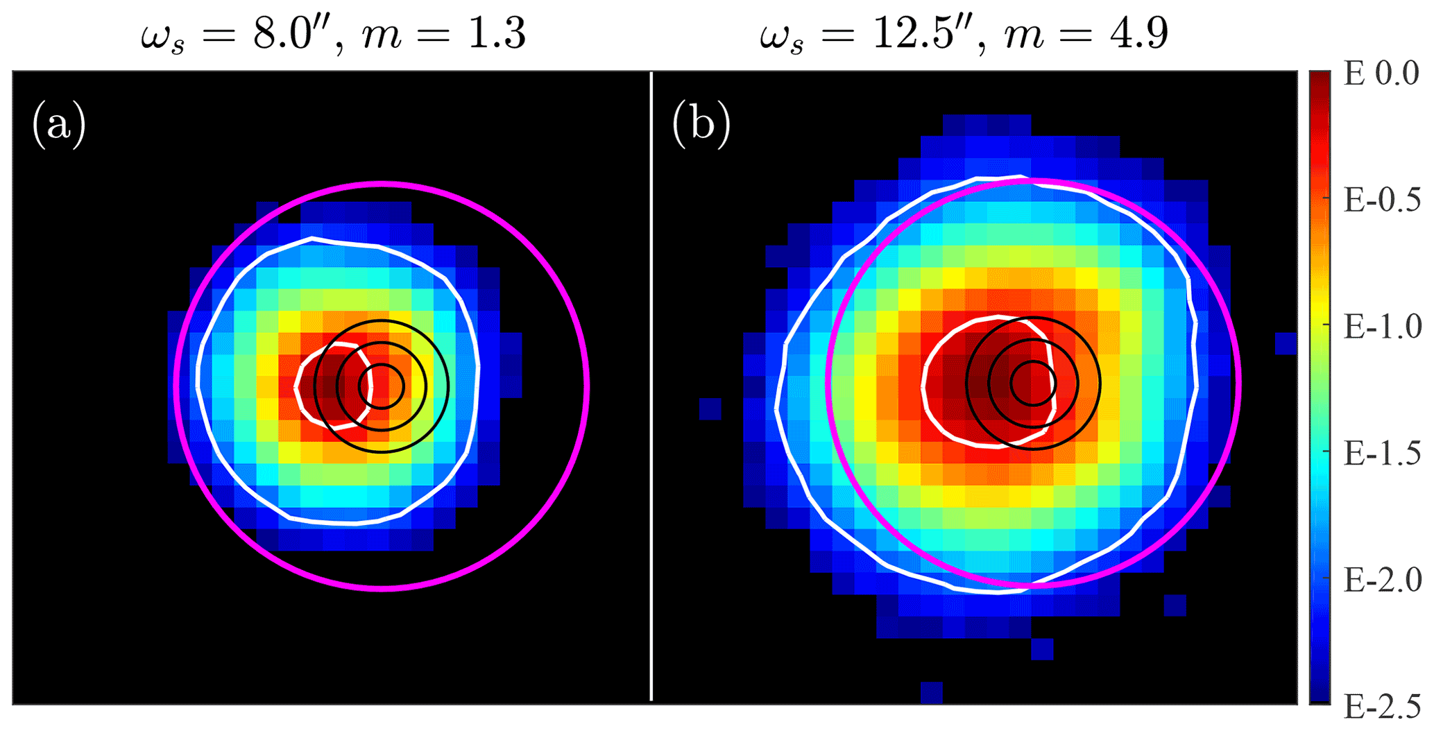
Figure C2 SPST09/C11 tracking of a 6 s short-exposure high-star spot (a) and low-star spot (b). These two illustrations represent high-resolution SBIG camera data that correspond to two Eureka points in Fig. 2 but whose respective air masses of 1.3 and 4.9 were obtained from the intersection of their ω_s values with the blue regression line. The fluxes shown in panels (a) and (b) are normalized to their maximum flux (their log-scale colour legend is shown on the right). The FOV, the 1 % and 50 % flux levels, and the centring tolerances are represented by a magenta circle, the two white contours, and the three black concentric circles (radius of 2, 4, and 6 arcsec), respectively. The spots are horizontally shifted by a 4 arcsec centring error with respect to the FOV. (Note that “′′” denotes arcseconds in this figure.)

Appendix D: Symbols and acronyms

Symbols
A, B, F, G	Spectral classes of stars
B	Instrument measurement of the sky background
bin	Several pixels read together
C	Instrument-specific photometric calibration parameter
c	Instrument-specific photometric conversion factor
cref	Ratio of photometric system references
cnt	Counts, instrument measurement unit
cgs	Centimetre–gram–second system of units
D	Telescope diameter (“aperture” in Table 1)
Deff	Particle effective diameter
Δ OSM	First-order OSM retrieval
Δ TSM	First-order TSM retrieval
ΔΔ TSM	Second-order TSM retrieval
ΔΩ	Solid FOV angle
dn	Atmospheric layer contribution to n
δϵ	Systematic observation errors
δB	Systematic B errors
δC	Systematic C errors
δc	Star-centring tolerance
δF	Systematic F errors
${\mathit{\delta }}_{M_{\mathrm{0}}}$	Systematic M0 errors
δR	Systematic R errors
δS	Systematic S errors
δt	Systematic time errors
δτ	Systematic τ errors
δx	Systematic x errors
e	Euler's natural number
e−	Electron
ϵ	Observation error
erg	cgs energy unit (1 erg $=\mathrm{1}\times {\mathrm{10}}^{-\mathrm{7}}$ J)
F	Attenuated star flux measurement
F0	Exoatmospheric star flux measurement
F0,cref	Exoatmospheric instrument measurement of the catalogue reference
F0,iref	Exoatmospheric instrument measurement of the instrument reference
Fe	Expected star signal at standard stabilized temperature
f	Telescope focal length
f#	Telescope focal number (focal ratio)
g	Aerosol asymmetry factor
g	Analogue–digital unit conversion factor
h	Observatory altitude above sea level
I	Attenuated star irradiance in absolute units
I0	Exoatmospheric star irradiance in absolute units
I0,cref	Exoatmospheric absolute irradiance of the catalogue reference
I0,iref	Exoatmospheric absolute irradiance of the instrument reference
k	Absorption index
kc	Conversion factor radians to arcseconds
kt	Turbulence parametrization constant
λ	Wavelength
M	Absolute attenuated magnitude
M0	Absolute exoatmospheric magnitude
M0,cref	Exoatmospheric catalogue magnitude of the catalogue reference
M0,iref	Exoatmospheric catalogue magnitude of the instrument reference

m	Air mass
$\stackrel{\mathrm{‾}}{\mathit{\omega }}$	Single-scattering albedo
ω	FWHM of the turbulence contribution to the long-exposure starspot
ωd	FWHM of the diffraction contribution to the starspot
ωs	FWHM of the turbulence contribution to the short-exposure starspot
${\mathit{\omega }}_{{\mathit{\theta }}_{\mathrm{L}}}$	FWHM of low-frequency jitter
Ω	FOV $/$ 2
P	Scattering phase function
Ps	Telescope plate scale
PΔΩ	Integral of normalized P over ΔΩ
px	Pixel
R	Rayleigh unit
R	Instrument measurement of the star irradiance
r0	Length parameter of the turbulence
rad	Radians
n	Refraction index
S	Instrumental attenuated magnitude
S0	Instrumental exoatmospheric magnitude
S0,cref	Exoatmospheric instrument magnitude of the catalogue reference
S0,iref	Exoatmospheric instrument magnitude of the instrument reference
s	Starspot off-axis or off-focus position
σ	Standard deviation
σθ	One-axis standard deviation of the total jitter
${\mathit{\sigma }}_{{\mathit{\theta }}_{\mathrm{L}}}$	Standard deviation of low-frequency jitter
t	Duration of an exposure
τ	Vertical (columnar) optical depth
θ	Zenith angle
θ	One-axis total starspot jitter
θL	One-axis low-frequency jitter
U, B, J	As V but for U, B, and J filters
V	M0 over the standard (visual) V filter
v	Wind speed
x	$m/\mathrm{0.921}$
z	Apparent zenith angle
zt	True zenith angle

Acronyms
AERONET	AErosol RObotic NETwork of Cimel sunphotometers
ADU	Analogue–digital unit
AOD	Aerosol optical depth
ASC	Aggregates of solid columns
a.s.l.	Above sea level
C11	Celestron C11 Schmidt-Cassegrain telescope
CCD	Charge-coupled device
CM	Coarse mode
COD	Cloud optical depth
Col	Solid columns
DEC(2000)	Declination at epoch 2000
DU	Dobson unit
FM	Fine mode
FOV	Field of view (of telescope, instrument)
FWHM	Full width at half maximum
GHM	General habit mixture
HG	Henyey–Greenstein phase function
HIP	Hipparcos star catalogue
Hp	Magnitude in Hipparcos photometric system
HR	Harvard revised photometry star catalogue
IBC1–4	Aurora brightness classes
Lum	Luminosity class of stars
M703	Alter M703 Maksutov-Cassegrain telescope made by Intes Micro
OD	Vertical (columnar) optical depth
[OI]	Neutral oxygen
OSM	One-star method of observation
PSF	Point spread function
PWV	Precipitable water vapour
RA(2000)	Right ascension at epoch 2000
SPST	Schulz & Partner STarphotometer (Schulz & Partner STernphotometer)
SPST05	Starphotometer serial, fifth instrument built by Dr. Schulz & Partner GmbH
SDA	Spectral deconvolution algorithm
SPST06	Starphotometer serial, same version as SPST05
SPST09	Starphotometer serial, upgraded version
Sp	Spectral class of stars
SSA	Single-scattering albedo
TEC	Thermoelectric cooler
TSM	Two-star method of observation
ZP	Zero-point of photometric system
WMO	World Meteorological Organization