the Creative Commons Attribution 4.0 License.
the Creative Commons Attribution 4.0 License.
 | 18 Oct 2021
Twenty-four-hour cloud cover calculation using a ground-based imager with machine learning
Joo Wan Cha
Ki-Ho Chang
In this study, image data features and machine learning methods were used to calculate 24 h continuous cloud cover from image data obtained by a camera-based imager on the ground. The image data features were the time (Julian day and hour), solar zenith angle, and statistical characteristics of the red–blue ratio, blue–red difference, and luminance. These features were determined from the red, green, and blue brightness of images subjected to a pre-processing process involving masking removal and distortion correction. The collected image data were divided into training, validation, and test sets and were used to optimize and evaluate the accuracy of each machine learning method. The cloud cover calculated by each machine learning method was verified with human-eye observation data from a manned observatory. Supervised machine learning models suitable for nowcasting, namely, support vector regression, random forest, gradient boosting machine, k-nearest neighbor, artificial neural network, and multiple linear regression methods, were employed and their results were compared. The best learning results were obtained by the support vector regression model, which had an accuracy, recall, and precision of 0.94, 0.70, and 0.76, respectively. Further, bias, root mean square error, and correlation coefficient values of 0.04 tenths, 1.45 tenths, and 0.93, respectively, were obtained for the cloud cover calculated using the test set. When the difference between the calculated and observed cloud cover was allowed to range between 0, 1, and 2 tenths, high agreements of approximately 42 %, 79 %, and 91 %, respectively, were obtained. The proposed system involving a ground-based imager and machine learning methods is expected to be suitable for application as an automated system to replace human-eye observations.
- Article
(5040 KB) - Full-text XML
- BibTeX
- EndNote


In countries, including South Korea, that have not introduced automated systems, ground-based cloud cover observation has been performed using the human eye, in accordance with the normalized synoptic observation rule of the World Meteorological Organization (WMO), and recorded in tenths or oktas (Kim et al., 2016; Yun and Whang, 2018). However, human-eye observation of cloud cover lacks consistency and depends on the observer conditions and the observation term (Mantelli Neto et al., 2010; Yang et al., 2016). Further, although continuous cloud cover observation during both day and night is important, there is a lack of data continuity (observations with at least 1 h intervals) because a person must perform direct observations (Kim and Cha, 2020). In addition, construction of a dense cloud observation network from observation environments with low accessibility, such as mountaintops, is difficult. Therefore, meteorological satellites and ground-based remote observation equipment that can continuously monitor clouds while overcoming these problems are now being employed (Yabuki et al., 2014; Yang et al., 2015; Kim et al., 2016; Kim and Cha, 2020).
Geostationary satellites can observe clouds on the global scale at intervals of several minutes; however, their spatial resolution is as large as several kilometers (Kim et al., 2018; Lee et al., 2018). Polar satellites have spatial resolutions of several hundred meters, i.e., high resolution; however, they can observe the same area only once or twice per day (Kim and Lee, 2019; Kim et al., 2020a). For both geostationary and polar satellites, geometric distortion problems occur during cloud cover estimation on the ground, depending on the cloud height (Mantelli Neto et al., 2010). As cloud heights and thicknesses vary, the cloud detection uncertainty also varies depending on the position of the sun or satellite (Ghonima et al., 2012). In general, cloud cover estimation using satellite data differs from the approach used for human-eye observation data, because the wide grid data around the central grid are averaged or calculated as fractions (Alonso-Montesinos, 2020; Sunil et al., 2021).
Radar, lidar, ceilometers, and camera-based imagers can be used as ground-based observation instruments (Boers et al., 2010). With regard to radar, cloud radar technology such as Ka-band radar is suitable for cloud detection but has the disadvantage of reduced detection accuracy with increased distance from the radar apparatus (Kim et al., 2020b; Yoshida et al., 2021). For lidar and ceilometers, the uncertainty is very large because the cloud cover is calculated from the signal intensity of a narrow portion of the sky (Costa-Surós et al., 2014; Peng et al., 2015; Kim and Cha, 2020). In contrast, for a camera-based imager, the sky in the surrounding hemisphere can be observed through a fisheye lens (180∘ field of view – FOV) mounted on the camera. Further, depending on the performance of the imager and the operation method, clouds can be observed continuously for 24 h, i.e., through the day and night. The data can be stored as images, and the cloud cover can be calculated from these data (Kim and Cha, 2020; Sunil et al., 2021).
Many studies have attempted to use camera-based imagers for automatic cloud observation and cloud cover calculation on the ground (Dev et al., 2016; Lothon et al., 2019; Shields et al., 2019). Those results can be used for numerical weather analysis and forecasting; they are also very economical and ideal for cloud monitoring over local areas (Mantelli Neto et al., 2010; Kazantzidis et al., 2012; Ye et al., 2017; Valentín et al., 2019). In general, cloud cover can be calculated based on the brightness of the red, green, and blue (RGB) colors of the image taken by the imager. In detail, the RGB brightness varies according to the light scattering from the sky and clouds, and, using the ratio or difference between these colors, cloud can be detected and cloud cover can be calculated (Long et al., 2006; Shields et al., 2013; Liu et al., 2014; Yang et al., 2015; Kim et al., 2016). For example, when the red–blue ratio (RBR) is 0.6 or more or the red–blue difference (RBD) is less than 30, the corresponding pixel is classified (i.e., using a threshold method) as a cloud pixel and incorporated in the cloud cover calculation (Kreuter et al., 2009; Heinle et al., 2010; Liu et al., 2014; Azhar et al., 2021). However, using these empirical methods, it is difficult to distinguish between the sky and clouds under various weather conditions (Yang et al., 2015). This is because the colors of the sky and clouds vary with the atmospheric conditions and because the sun position and threshold conditions can change continuously (Yabuki et al., 2014; Blazek and Pata, 2015; Cazorla et al., 2015; Calbó et al., 2017). Therefore, methods of cloud detection and cloud cover calculation involving application of machine learning methods to images are now being implemented, as an alternative to empirical methods (Peng et al., 2015; Lothon et al., 2019; Al-lahham et al., 2020; Shi et al., 2021).
Cloud cover can be calculated from camera-based imager data using a supervised machine learning method capable of regression analysis (Al-lahham et al., 2020). Supervised learning is a method through which a prediction model is constructed using training data which already contain the labeled data. Examples include support vector machines (SVMs), decision trees (DTs), gradient boosting machines (GBMs), and artificial neural networks (ANNs) (Çınar et al., 2020; Shin et al., 2020). Deep learning methods that repeatedly learn data features by sub-sampling image data at each convolution step for gradient descent are also available, such as convolutional neural networks (Dev et al., 2019; Shi et al., 2019; Xie et al., 2020). However, this approach is difficult to utilize for nowcasting because considerable physical resources and time are consumed by the learning and prediction processes (Al Banna et al., 2020; Kim et al., 2021).
In this study, cloud cover was calculated continuously for 24 h from image data obtained by a camera-based imager on the ground, using image data features and machine learning methods. ANN, GBM, k-nearest neighbor (kNN), multiple linear regression (MLR), support vector regression (SVR), and random forest (RF) methods suitable for nowcasting were used for calculation. For each of these methods, an optimal prediction model is constructed by setting hyper-parameters. The machine learning model most suitable for cloud cover calculation is then selected by comparing the prediction performance of each model on training and validation datasets. The cloud cover calculated from the selected machine learning model is then compared with human-eye observation data and the results are analyzed. The remainder of this paper is organized as follows. The image and observation data used in this study are described in Sect. 2, and the machine learning methods and their sets are summarized in Sect. 3. The prediction performance evaluation for each machine learning method and the calculation result verification are reported in Sect. 4. Finally, the summary and conclusion are given in Sect. 5.
2.1 Ground-based imager
In this study, a digital camera-based automatic cloud observation system (ACOS) was developed using a Canon EOS 6D camera to detect and calculate cloud cover for 24 h, as shown in Fig. 1. This system was developed by the National Institute of Meteorological Sciences (NIMS)/Korea Meteorological Administration (KMA) and A & D ⋅ 3D Co., Ltd. (Kim and Cha, 2020). The ACOS was installed at the Daejeon Regional Office of Meteorology (DROM; 36.37∘ N, 127.37∘ E), a manned observatory in which cloud cover observation by human eye is performed. The detailed ACOS specifications are listed in Table 1. The International Organization for Standardization (ISO) values of the complementary metal oxide semiconductor (CMOS) sensor employed in the camera are 100 (day)–25 600 (night), and the sensitivity is adjusted according to the image brightness. In this study, the camera shutter speed was set to s (day)–5 s (night), considering the long exposure for object detection required at night. The F-stop value was set to F8 (day)–F11 (night), and the sky-dome object was taken with a large depth of field (Peng et al., 2015; Dev et al., 2017). The camera lens was installed at a height of 1.8 m, similar to human-eye height, and a fisheye lens (EF 8–15 mm F/4L fisheye USM) was installed to capture the entire surroundings, including the sky and clouds, within a 180∘ FOV. To perform 24 h continuous observation, heating (below −2 ∘C) and ventilation devices were installed inside the ACOS body to facilitate image acquisition without manned management (Dev et al., 2015; Kim and Cha, 2020).
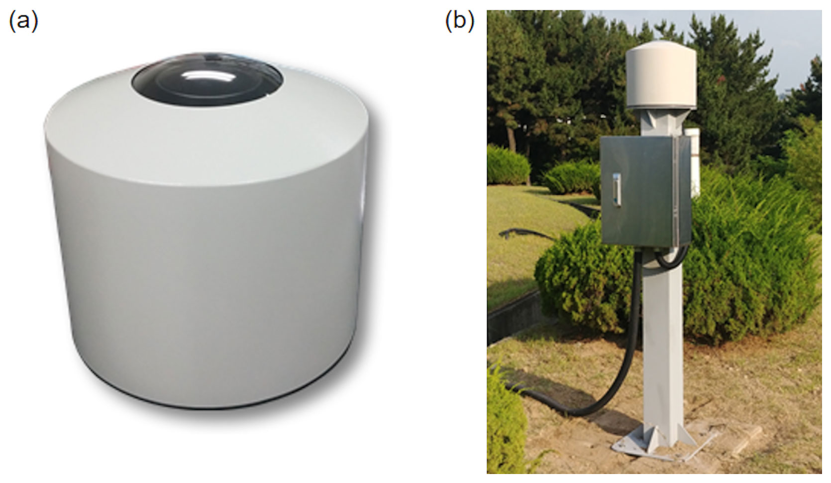
Figure 1ACOS appearance (a) and installation environment (b) (Kim and Cha, 2020).

2.2 Cloud cover calculation and validation
The image data captured by ACOS were processed by converting each RGB channel of each image pixel to a brightness of 0–255. Although the camera-lens FOV was 180∘, only pixel data within the zenith angle of 80∘ (FOV 160∘) were used. This condition was in consideration of the permanent masking area of the horizontal plane due to surrounding objects (buildings, trees, equipment, etc.) (Kazantzidis et al., 2012; Shields et al., 2019; Kim and Cha, 2020). For cloud cover calculation using the ACOS images, image data taken at 1 h intervals from 1 January to 31 December 2019 were used. The cloud cover was calculated using the statistical characteristics of the RGB brightness ratio (i.e., the red–blue ratio – RBR), difference (i.e., the blue–red difference – BRD), and luminance (Y), which vary for each image (Sect. 2.3), as well as supervised machine learning methods (Sect. 3). Here, Y was calculated as (Sazzad et al., 2013; Shimoji et al., 2016). The calculated cloud cover was compared with human-eye observation data from DROM. As the cloud cover was calculated as a percentage between 0 % and 100 %, the result was converted to an integer (tenth) between 0 and 10 (Table 2) for comparison with the human-eye-based cloud cover values. As the ACOS was installed at DROM, there were no location differences between observers; thus, the same clouds were captured (Kim and Cha, 2020). At DROM, night observations were performed at 1 h intervals during inclement weather (rainfall, snowfall, etc.), but otherwise at 3 h intervals. The night period varied with the season. Considering this, a total of 7402 images of concurrent human observations were collected, excluding missing cases, from the ACOS.
Table 2ACOS cloud cover (%) to DROM human-eye-observed cloud cover (tenths) conversion table.

The entire collected dataset was randomly sampled without replacement. Overall, 50 % (3701 cases) of the total data elements were configured as a training set, 30 % (2221 cases) as a validation set, and 20 % (1480 cases) as a test set (Xiong et al., 2020). The training set was used to train the machine learning algorithms, and the prediction performance of each machine learning method was assessed using the validation set. Optimal hyper-parameters were set for each machine learning method through the training and validation sets. The results of each machine learning method were compared. In this process, the test set was input to the machine learning model that exhibited the best prediction performance, and the calculated results and human-eye observation data were compared. The accuracy, recall, precision, bias, root mean square error (RMSE), and correlation coefficient (R) were analyzed according to Eqs. (1)–(6); hence, the prediction performance of each machine learning method was determined and compared based on the human-eye observation data.
Here, TP, TN, FP, and FN are the number of true positives (reference: yes, prediction: yes), true negatives (reference: yes, prediction: no), false positives (reference: no, prediction: yes), and false negatives (reference: no, prediction: no), respectively. Further, M, O, and N are the cloud cover calculated by the employed machine learning method, the human-eye-observed cloud cover, and the number of data, respectively.
2.3 Machine learning input data
The data input to the machine learning algorithms for cloud cover calculation using the ACOS images were produced as follows. First, as the ACOS image was taken with a fisheye lens, the image was distorted. That is, objects at the edge were smaller than those at the center of the image (Chauvin et al., 2015; Yang et al., 2015; Lothon et al., 2019). Therefore, the relative size of each object in the image was adjusted through orthogonal projection distortion correction according to the method expressed in Eqs. (7)–(11) (Kim and Cha, 2020).
where r is the distance between the center pixel (cx, cy) of the original image and each pixel (x, y), θ is the solar zenith angle (SZA), “radi” is the image radius (distance between center and edge pixel of circular images), ϕ is the azimuth, and x′ and y′ are the coordinates of each pixel after distortion correction.
Second, surrounding masks such as buildings, trees, and equipment, as well as light sources such as the sun, moon, and stars, were removed from the image (building, tree, and equipment: masking was performed when the mean RGB brightness was less than 60 in the daytime on a clear day; light source: masking was performed when the mean RGB brightness exceeded 240). These objects directly mask the sky and clouds or make it difficult to distinguish them; therefore, they must be removed when calculating cloud cover (Yabuki et al., 2014; Kim et al., 2016; Kim and Cha, 2020). Third, the RBR, BRD, and Y frequency distributions were calculated using the RGB brightness of each pixel of image data subjected to pre-processing (i.e., masking removal and distortion correction). The class interval sizes of the RBR, BRD, and Y frequency distributions were set to 0.02, 2, and 2, respectively, and classes with frequencies of less than 100 were ignored. Statistical characteristics of the mean, mode, frequency of mode, kurtosis, skewness, and quantile (Q0–Q4: 0 %, 25 %, 50 %, 75 %, and 100 %) data obtained for each frequency distribution were used as input for each machine learning method. As input data for machine learning, time information (Julian day and hour) allowed differentiating seasons and day and night. Further, SZA should be considered because the colors of the sky and clouds change according to the position of the sun (Blazek and Pata, 2015; Cazorla et al., 2015; Azhar et al., 2021). As these image data features have different appearances under different conditions (cloud cover, day, night, etc.), they constitute an important variable in machine learning regression for cloud cover calculation (Heinle et al., 2010; Li et al., 2011).
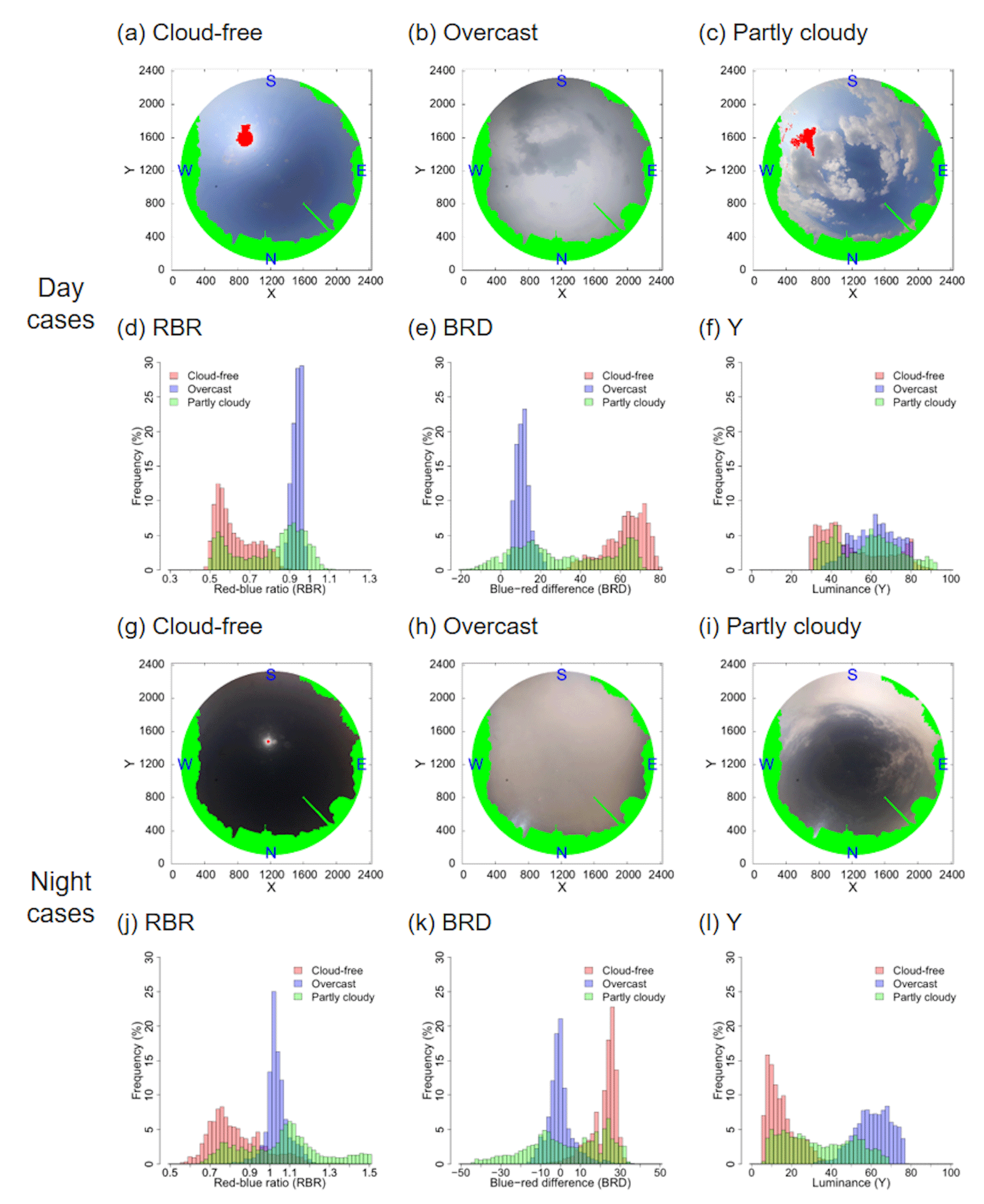
Figure 2Distortion-corrected images and RBR (d, j), BRD (e, k), and Y (f, l) relative frequency distributions for cloud-free (0 tenths), overcast (10 tenths), and partly cloudy (5 tenths) cases at day and night. The daytime cloud-free (a), overcast (b), and partly cloudy (c) data were obtained at 14:00 LST on 8 March, 12:00 LST on 15 July, and 15:00 LST on 28 September 2019. Cloud-free (g), overcast (h), and partly cloudy (i) nighttime data were obtained at 03:00 LST on 24 January, 20:00 LST on 18 February, and 22:00 LST on 30 April 2019. The green and red areas are masked to remove surrounding masks (i.e., buildings, trees, and equipment) and light sources (i.e., the sun and moon), respectively.
Figure 2 shows distortion-corrected images for day and night cloud-free, overcast, and partly cloudy cases and the RBR, BRD, and Y relative frequency distributions. The frequency distributions were expressed as percentages over approximately 310 000 px excluding the masked area. Human-eye observations at DROM yielded cloud-free (Fig. 2a and g), overcast (Fig. 2b and h), and partly cloudy (Fig. 2c and i) case values of 0, 10, and 5 tenths, respectively. As for the RBR frequency distribution during the day, larger RBR distributions were observed for the overcast than cloud-free case, and bimodal distributions including both (i.e., overcast and cloud-free) distributions were obtained for the partly cloudy case. The variance was large in the partly cloudy case. With regard to the BRD frequency distribution, the blue-channel brightness increased with Rayleigh scattering, such that the cloud-free case with many sky pixels had larger BRD distribution than the overcast case (Ghonima et al., 2012; Kim et al., 2016). In contrast, the Y frequency distribution was relatively large for the overcast case, which involved many cloud pixels. Although the RBR frequency distributions at night and day were similar, the RBR was larger at night because the red-channel brightness increased under the influence of Mie scattering (Kyba et al., 2012; Kim and Cha, 2020). A negative BRD distribution was obtained from the cloud pixels. At night, there is no light source such as the sun. Therefore, in this study, RGB brightness close to black (0, 0, 0) was distributed in the cloud-free case, yielding small Y. As the images obtained through ACOS had different RBR, BRD, and Y frequency distribution classes and shapes for each case, it was necessary to train these data features (i.e., the mean, mode, frequency of mode, kurtosis, skewness, and quantile of each frequency distribution) on a machine learning model to calculate the cloud cover.
Depending on the machine learning method, even if the accuracy, recall, precision, and R of the trained model are high and the bias and RMSE are small, overfitting problems may occur when data other than training data are used for prediction; these problems can yield low prediction performance (Ying, 2019). Therefore, in this study, optimal hyper-parameters were set by iteratively changing the hyper-parameter for each machine learning method using the training and validation sets (Bergstra and Bengio, 2012). The optimal hyper-parameter was determined based on the accuracy, recall, precision, bias, RMSE, and R, which were prediction performance indicators for each iteration. The details and hyper-parameter settings of each supervised machine learning method used in this study are described in Sect. 3.1 to 3.6. The prediction results of each machine learning method are compared in Sect. 4.1.
3.1 Multiple linear regression (MLR)
The method in which the relationship of the dependent variable to the independent variable is regressed by considering one independent variable only is called simple linear regression, and the method in which the change in the dependent variable is predicted based on the changes in two or more independent variables is called MLR. An MLR model with k independent variables predicts the dependent variable as shown in Eq. (12), using the least squares method which minimizes the predictor variable and the sum of squared errors (Fig. 3a) (Olive, 2017). In this study, we used the R “glm” package (Geyer, 2003).
where βk are the population coefficients (i.e., parameters), and Xki is the kth predictor of the ith observation (a value that describes the variable Yi to be predicted). In this study, the independent variables were the RGB, BRD, and Y mean, mode, frequency of mode, skewness, kurtosis, quantile, as well as the Julian day, hour, and SZA. The dependent variable was the cloud cover observed by human eyes.

Figure 3Schematic of each machine learning method: MLR (a), kNN (b), SVR (c), ANN (d), RF (e), and GBM (f).
3.2 k-nearest neighbor (kNN)
The kNN method involves non-parametric, instance-based learning and is one of the simplest predictive models in machine learning. The kNN algorithm finds the k-nearest neighbors to the query in the data feature space, as shown in Fig. 3b, and then predicts the query with distance-based weights (S. Zhang et al., 2018). That is, a set of independent variables is constructed as a cluster, and values corresponding to each neighbor are weighted according to the Euclidean distance and predicted (Martínez et al., 2019). In this study, the R “class” package (Ripley and Venables, 2021a) was used, and the hyper-parameter setting was k=15.
3.3 Support vector regression (SVR)
SVR is an extended method that can be used for regression analysis by introducing an ε-insensitive loss function to an SVM. As shown in Fig. 3c, a hyperplane consisting of support vectors that can classify the maximum margin for the distance between vectors is found (Gani et al., 2010; Taghizadeh-Mehrjardi et al., 2017). The optimal hyperplane is obtained by finding w and b that minimize the mapping function (Φ(w)), as shown in Eq. (13) (Meyer, 2001). The constraints are shown in Eq. (14). Then, as in Eq. (15), the kernel is applied and mapped to a higher dimension. Here, ε determines the threshold of margin, ξ is a slack variable to allow error, and C is the allowable cost that can violate the constraint of Eq. (14). In this study, the R “e1071” package (Meyer et al., 2021) was used, the SVR kernel was set as a radial basis function (RBF), and the hyper-parameters were set to epsilon (ε)=0.12, gamma (γ)=0.04, and cost (C)=5.
where subscript i and j are ith and jth data point, respectively, and γ is a parameter that controls the RBF kernel width.
3.4 Artificial neural network (ANN)
An ANN is a mathematical model that mimics a neuron; i.e., the signal transmission system of a biological neural network. As shown in Fig. 3d, this model consists of an input layer that receives input data, an output layer that outputs prediction results, and an invisible hidden layer between the two layers (Rosa et al., 2020). The hidden node of the hidden layer acts like a neuron in a neural network and is composed of weight, bias, and an activation function. In this study, we used the R “nnet” package (Ripley and Venables, 2021b), which is based on feed-forward neural networks with a single hidden layer that can rapidly learn and predict while considering nowcasting. The hyper-parameters of this package were set as follows: size (number of hidden nodes) = 7, maxit (maximum number of iterations) = 700, and decay (weight decay parameter) = 0.05.
3.5 Random forest (RF)
The RF method composes N decision trees by combining randomly selected variables from each node to grow a regression tree, as shown in Fig. 3e. An ensemble of the results of each decision tree is obtained, and hence a prediction result is provided (Wright and Ziegler, 2017). That is, in the RF ensemble learning method, every individual tree of the decision tree contributes to the final prediction (Shin et al., 2020; Kim et al., 2021). In this study, the R “Ranger” package (Wright et al., 2020) was used, and the hyper-parameters were set to num.trees (the number of trees) = 510, mtry (the number of variables randomly sampled from each node) = 7, and min.node.size (minimal node size) = 5.
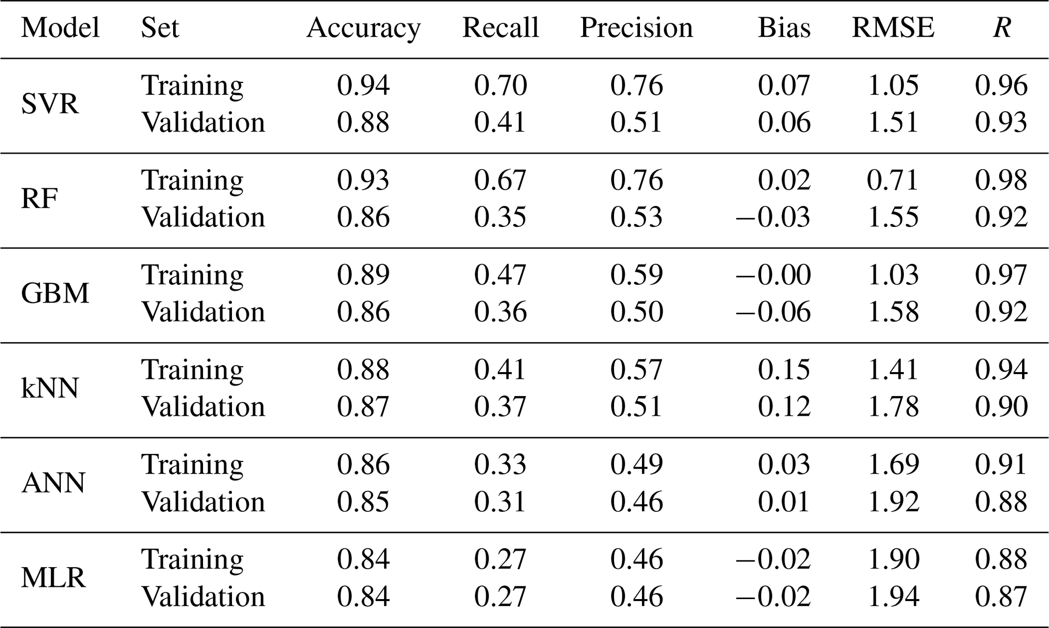
Table 3Prediction performance for all cloud cover of machine learning methods using training and validation sets.
3.6 Gradient boosting machine (GBM)
The GBM uses boosting instead of bagging during resampling and ensemble processes. As shown in Fig. 3f, a model with improved predictive power is created by gradually improving upon the parts that the previous model could not predict while sequentially generating weak models. The final prediction is calculated from the weighted mean of these results (Friedman, 2001). In other words, gradient boosting updates the weights iteratively to minimize the difference from the function f(x) that predicts the actual observation using gradient descent (Ridgeway, 2020). In this study, the R “gbm” package (Greenwell et al., 2020) was used; the GBM kernel was set to a Gaussian distribution function; and the hyper-parameters were set to n.trees (number of trees) = 500, interaction.depth (maximum depth of binary tree) = 5, and shrinkage (learning rate) = 0.1.
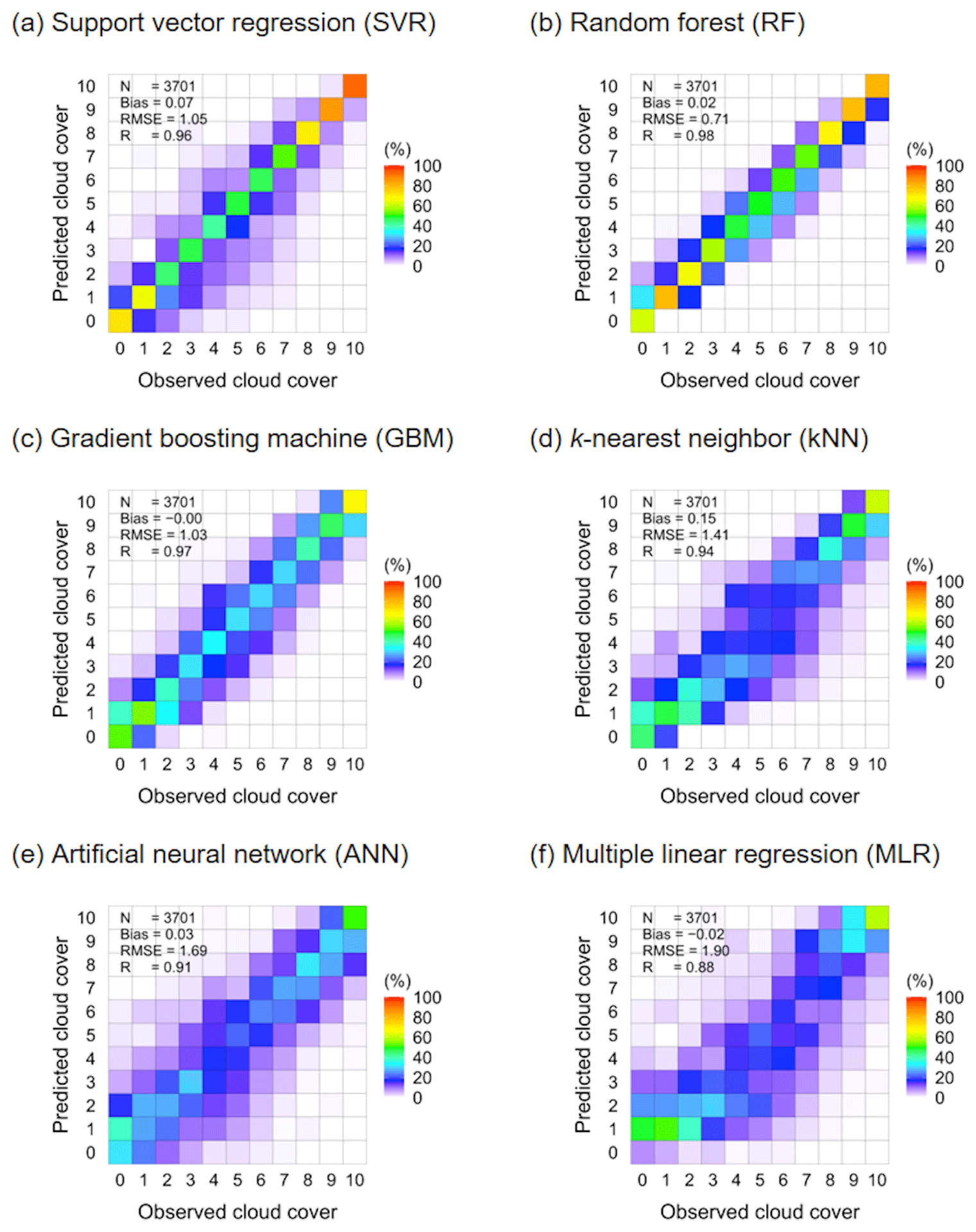
Figure 4Scatter plots of observed cloud cover and that predicted by machine learning methods – SVR (a), RF (b), GBM (c), kNN (d), ANN (e), and MLR (f) – on the training set. The number of observations for each observed cloud cover are 0: 992, 1: 136, 2: 141, 3: 156, 4: 149, 5: 135, 6: 221, 7: 271, 8: 320, 9: 441, and 10: 739.
4.1 Training and validation results of machine learning methods
Figure 4 shows the cloud cover prediction results obtained using the training set for each machine learning method. The hyper-parameters were optimized using the training and validation sets. Each box in the figure denotes the ratio (%) of the number of observations for each cloud cover in the DROM and the number of predictions for each cloud cover in the SVR model. The higher the frequency in the diagonal one-to-one boxes, the better the agreement between the observed and predicted cloud cover. In other words, the closer the diagonal one-to-one boxes are to red (i.e., 100 %), the higher is the agreement. For the training set, the highest human-eye observation data frequency by cloud cover was 26.80 % at 0 tenths; this was followed by 19.97 % at 10 tenths and 3.65 %–11.92 % at 1–9 tenths. For the SVR model, the 0- and 10-tenth frequencies were 71.88 % and 92.15 %, respectively, with the agreement being greatest among the machine learning models. As detailed in Table 3, the SVR accuracy, recall, and precision for all cloud cover were 0.94, 0.70, and 0.76, respectively, indicating the best prediction performance. The accuracy was in the range of 0.91–0.98 for each cloud cover, whereas recall and precision were in the ranges of 0.42–0.92 and 0.24–0.99, exhibiting low predictive power in the partly cloudy case. The bias was 0.07 tenths, the RMSE was 1.05 tenths, and R was 0.96. In the case of the RF model, the 0- and 10-tenth frequencies were 61.79 % and 80.65 %, respectively, being lower than those of the SVR model; however, the prediction for 1–9 tenths exhibited high agreement to within ±1 tenth. The accuracy, recall, and precision were 0.93, 0.67, and 0.76, respectively, which is lower than SVR model, but the bias and RMSE were the smallest at 0.02 and 0.71 tenths, respectively, and the R value was the highest at 0.98. However, for the validation set, the SVR model prediction performance (accuracy: 0.88, recall: 0.41, precision: 0.51, bias: 0.06 tenths, RMSE: 1.51 tenths, and R: 0.93) was better than that of the RF model. In other words, the RF model exhibited a tendency to overfit in this study. The accuracy of these results exceeds that of the classification machine learning method (0.60–0.85) presented by Dev et al. (2016) using day and night image data, and it is higher than or similar to the accuracy (0.91–0.94) achieved using the regression and deep learning machine learning methods proposed by Shi et al. (2019, 2021) for day and night image data. Apart from the SVR and RF methods, the machine learning methods exhibited similar frequency distributions; however, the accuracy, recall, precision, and R were lower and the RMSE values were higher in the order of GBM, kNN, ANN, and MLR. In particular, the MLR model had very poor predictive power (accuracy: 0.75, recall: 0.08, and precision: 0.78) for 0 tenths using the training set.
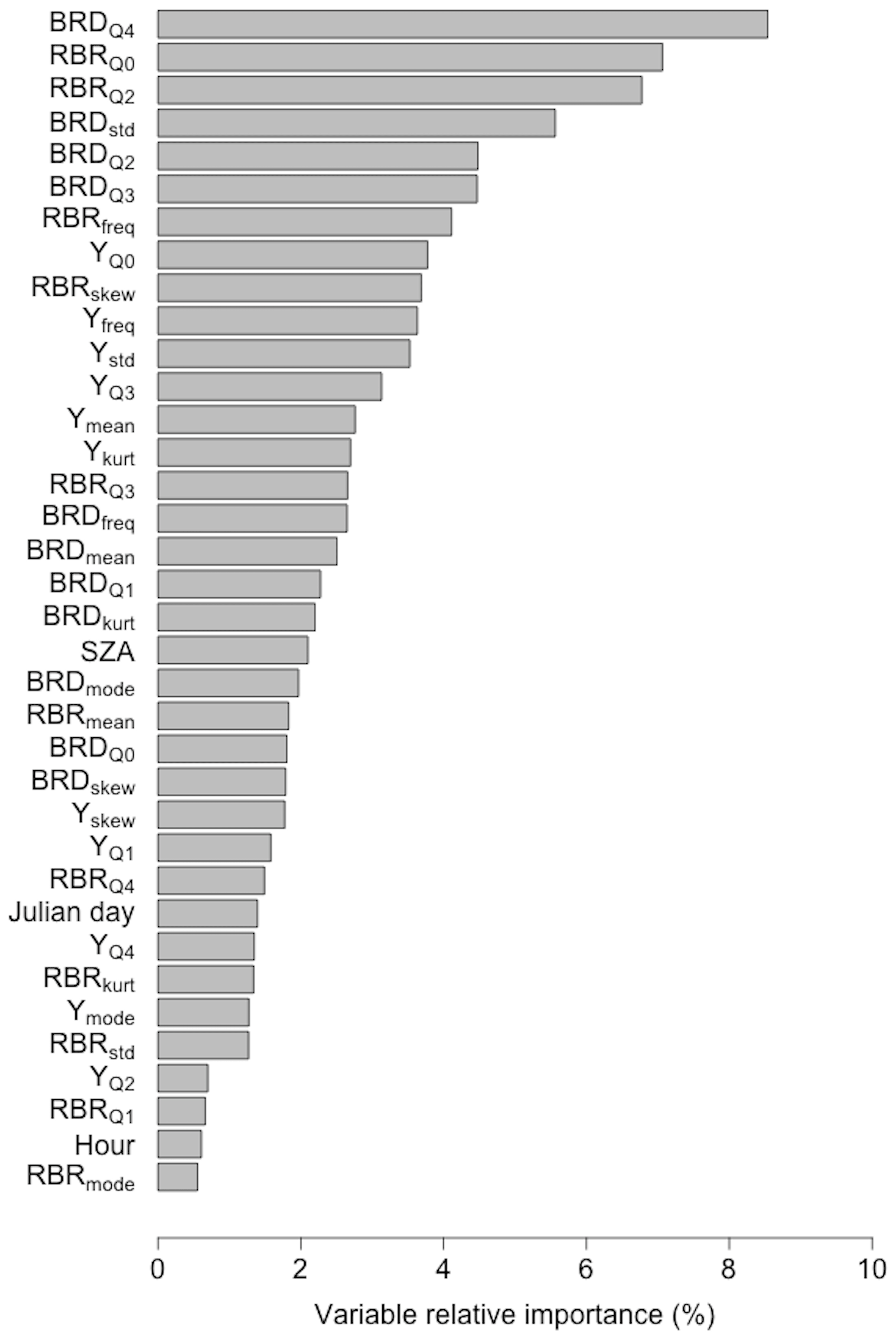
The relative importance of the input variable of the SVR method, which exhibited the best predictive performance in this study, is shown in Fig. 5. BRD had the highest relative importance at 8.54 %, whereas RBRmode had the lowest importance at 0.55 %. Among the RBR data features, RBR had the highest importance at 7.06 %, and, among the Y data features, had the highest importance at 3.78 %. In terms of the cumulative relative importance, the BRD-, RBR- and Y-related data features contributed 38.25 %, 31.44 %, and 26.20 % of the total (100 %), respectively, to the cloud cover prediction, and the remaining data features contributed 4.10 %. The relationship between input data features is complex to determine the optimal hyperplane of the SVR model, and the variable importance is determined so that the cloud cover can be calculated with the smallest error using the observed cloud cover (Singh et al., 2020). Even if the BRD-related data features have the same RBR characteristics, they contribute to machine learning more comprehensively by day, night, and cloud presence depending on the BRD value; therefore, they are critical to cloud cover calculation. By contrast, the Y-related data feature is sensitive to the RGB brightness (especially the G brightness) in the image, but the difference in the Y characteristics according to the cloud cover during the day was not large; thus, their importance was relatively low. Although time information and SZA can provide information such as daytime, nighttime, and sunset/sunrise images, they have the lowest importance because they do not have statistical characteristics that can be used to directly calculate cloud cover. The importance of these data features may vary depending on the camera's sensor (Kazantzidis et al., 2012).
4.2 Test set results for SVR model
Figure 6 shows the total cases and seasonal scatter plots of the DROM cloud cover and the ACOS cloud cover prediction calculated from the SVR model using the test set. In the Korean Peninsula, the winter cloud cover is sparse (<5 tenths) as the weather is generally clear because of the Siberian air mass. In summer, the rainy season is concentrated under the influence of the Yangtze River and Pacific air masses, and the cloud cover is dense (>5 tenths) until fall because of typhoons (Kim and Lee, 2018; Kim et al., 2020a). Furthermore, the Korean Peninsula experiences a westerly wind, cumulus heat generated in the western sea moves inland, and the cloud cover changes rapidly and continuously (Kim et al., 2021). The cloud cover distributions calculated for all test set cases exhibited good agreement with the observed cloud cover, with accuracy, recall, and precision of 0.88, 0.42, and 0.52, respectively. Further, the bias, RMSE, and R were 0.04 tenths, 1.45 tenths, and 0.93, respectively. In fall, the bias, RMSE, and R were −0.12 tenths, 1.30 tenths, and 0.95, respectively, indicating that the difference between the observed and calculated cloud cover was small. In winter and summer, the RMSE was larger and R was lower than in the other seasons. This is because the cloud cover calculation error is large at sunrise and sunset (100∘ ≥ SZA > 80∘), i.e., where daytime (SZA ≤ 80∘) and nighttime (SZA > 100∘) intersect (Lalonde et al., 2010; Alonso et al., 2014; Kim and Cha, 2020).
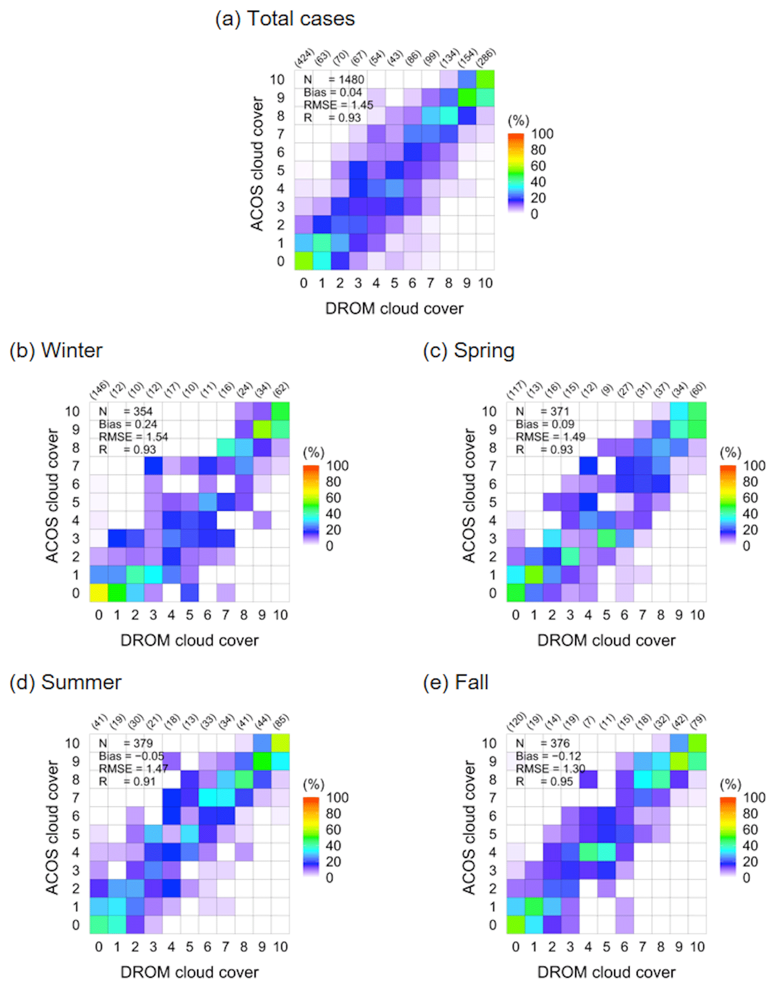
Figure 6Scatter plots of total (a) and seasonal (b–e) cloud cover based on observed (DROM) and calculated (ACOS) cloud cover for the test set. Parentheses values are the number of observations for each cloud cover in DROM.
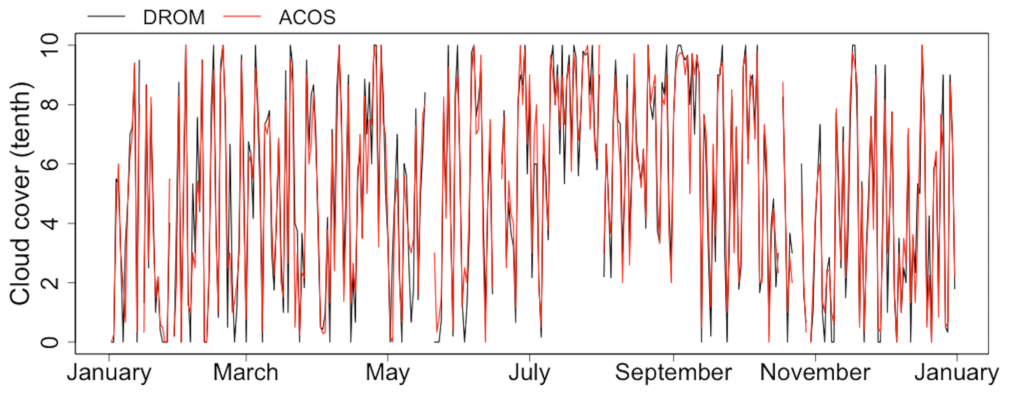
Figure 7Daily mean time series of observed (DROM) and calculated (ACOS) cloud cover for the test set.
For the test set daytime cases, the bias, RMSE, and R were 0.10 tenths, 1.20 tenths, and 0.95, respectively, and 0.08 tenths, 1.59 tenths, and 0.93, respectively, for the night data. However, for sunrise and sunset, these values were −0.22 tenths, 1.71 tenths, and 0.90, respectively. Relatively, the bias and RMSE were large and R was low. In spring and autumn, sunrise and sunset images were learned at similar times (sunrise: 06:00–07:00 LST, sunset: 18:00–19:00 LST); however, differences between the winter (sunrise: 07:00–08:00 LST, sunset: 17:00–18:00 LST) and summer (sunrise: 05:00–06:00 LST, sunset: 19:00–20:00 LST) results are apparent because sunrise and sunset occurred late or early and exhibited different features from the data features learned for those times (Liu et al., 2014; Li et al., 2019). That is, owing to the sunrise/sunset glow, high cloud cover calculation errors are obtained at sunrise/sunset, when it is difficult to distinguish between the sky and clouds because of the reddish sky on a clear day and the bluish cloud on a cloudy day (Kim et al., 2021). Therefore, for the test set, the bias, RMSE, and R for sunrise and sunset in spring and autumn were −0.24 tenths, 1.46 tenths, and 0.93, respectively. However, in winter and summer, the bias, RMSE, and R were −0.21 tenths, 1.93 tenths, and 0.86, respectively. Nevertheless, the results of this study surpass those of Kim et al. (2016) for daytime (08:00–17:00 LST; bias: −0.36 tenths, RMSE: 2.12 tenths, R: 0.87) and Kim and Cha (2020) for nighttime (19:00–06:00 LST; bias: −0.28 tenths, RMSE: 1.78 tenths, R: 0.91) cases. Shields et al. (2019) employed different day and night cloud cover calculation algorithms. In that approach, cloud cover calculation errors may occur at sunrise and sunset. Therefore, if a day and night continuous cloud cover calculation algorithm is considered, the calculation error for this discontinuous time period should be reduced (Huo and Lu, 2009; Li et al., 2019). Figure 7 shows the daily mean cloud cover results based on the observed and calculated cloud cover for the test set. For the observed and calculated cloud cover, a bias of 0.03 tenths, RMSE of 0.92 tenths, and R of 0.96 were obtained. The coefficient of determination (R2) was 0.92, and the result calculated from the SVR model constructed in this study explained approximately 92 % of the observed data in the test set.
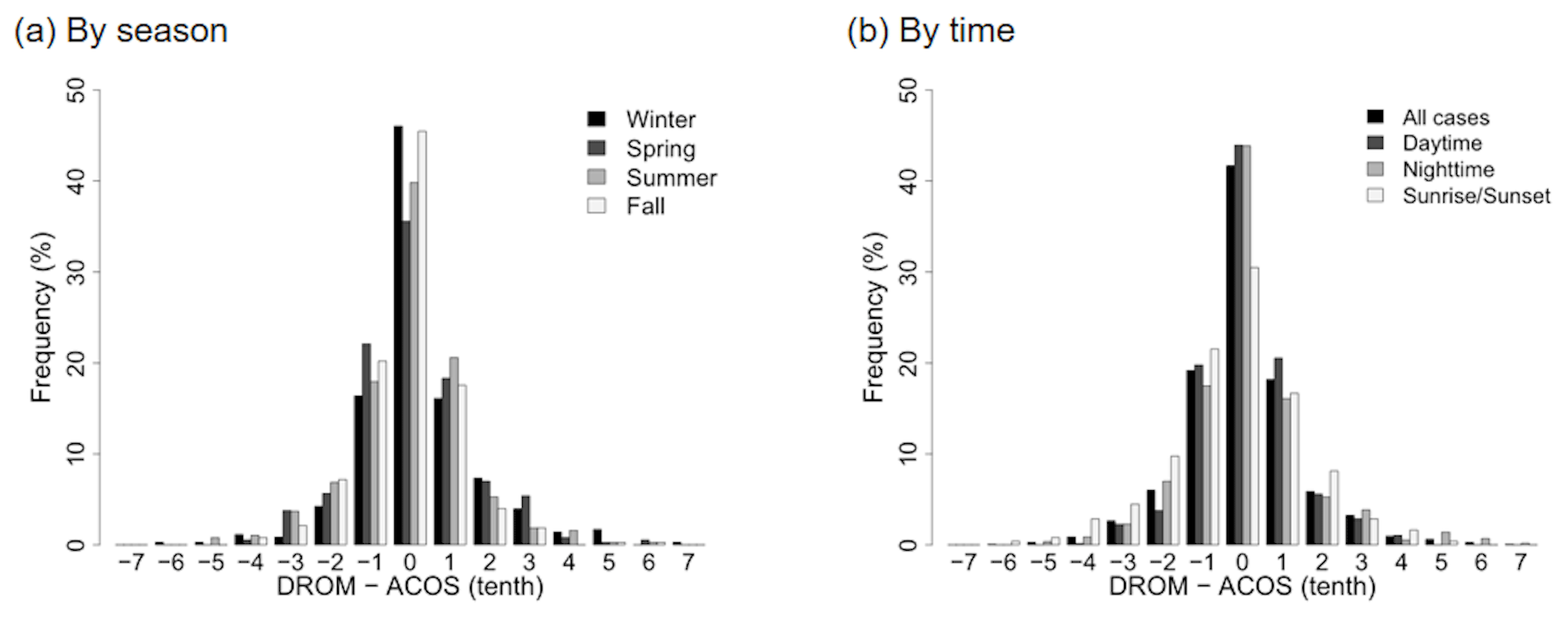
Figure 8Relative frequency distributions of differences between observed (DROM) and calculated (ACOS) cloud cover by season and time for the test set.
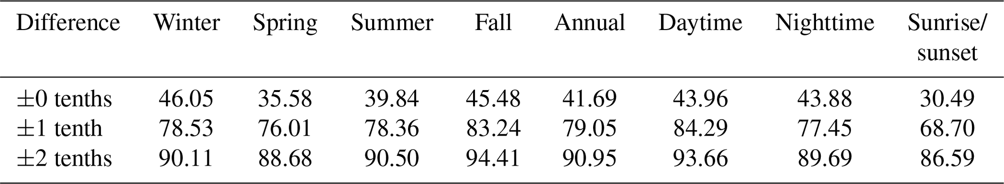
Figure 8 shows the frequency distribution of the differences between ACOS and DROM by season and time. In this frequency distribution, the higher the 0-tenth frequency, the higher the agreement between the observed and calculated cloud cover. The highest 0-tenth frequency was obtained in winter (46.05 %) and the lowest in spring (35.58 %), but 41.69 % agreement was obtained for all seasons. Conditioned on the time of day, high agreement of approximately 44 % was obtained for both daytime and nighttime, but the lowest agreement (30.49 %) was obtained for sunrise and sunset. Previous studies obtained a difference of approximately 2 tenths from the observed cloud cover for the cloud cover calculated based on the ground-based imager data (Kazantzidis et al., 2012; Kim et al., 2016; Kim and Cha, 2020; Wang et al., 2021). When a difference of up to 2 tenths was allowed between the observed and calculated cloud cover, the agreement was 90.95 %, as detailed in Table 4. When a difference up to 1 tenth between both cloud cover results was allowed for all cases, the agreement was 79.05 %. When the difference was within 2 tenths, high agreement of 86.59 % to 94.41 % by season and by time was obtained. These results reveal greater agreement than those obtained by Cazorla et al. (2008), Kreuter et al. (2009), Kazantzidis et al. (2012), Kim et al. (2016), Krinitskiy and Sinitsyn (2016), Fa et al. (2019), Kim and Cha (2020), Xie et al. (2020), and Wang et al. (2021). In those works, 80 %–94 % agreement was achieved when the allowed difference between the observed and calculated cloud cover was 2 oktas (2.5 tenths) or 2 tenths for day, night, and day and night cases.
Table 4Concordance frequency (%) according to the difference between the observed (DROM) and calculated (ACOS) cloud cover for the test set.
In this study, data features of images captured using ACOS, a camera-based imager on the ground, were used in conjunction with machine learning methods to continuously calculate cloud cover for 24 h, at day and night. The data features of the images used as the machine learning input data were the mean, mode, frequency of mode, skewness, kurtosis, and quantile (Q0–Q4) of the RBR, BRD, and Y frequency distributions, respectively, along with the Julian day, hour, and SZA. The RBR, BRD, and Y data features were calculated through pre-processing using the methods described by Kim and Cha (2020) (masking removal and distortion correction). These features indicate the sky and cloud colors depending on the light scattering characteristics in the day and night, along with the presence or absence of clouds and the position of the sun (Heinle et al., 2010; Blazek and Pata, 2015; Li et al., 2019). The collected image data (100 %) were composed of training (50 %), validation (30 %), and test (20 %) sets and were used for optimization of the models produced by the machine learning methods, comparative analysis of the prediction results of each machine learning method, and verification of the predicted cloud cover. In this study, the SVR, RF, GBM, kNN, ANN, and MLR supervised machine learning methods were used. Among these methods, the SVR model exhibited the best prediction performance, with accuracy, recall, and precision of 0.94, 0.70, and 0.76, respectively. The cloud cover calculation results produced by the SVR on the test set had a bias of 0.04 tenths, RMSE of 1.45 tenths, and R of 0.93. With respect to this calculation result, when a difference of 2 tenths from the observed cloud cover was allowed, the agreement was 41.69 %, 79.05 %, and 90.95 % for 0-, 1-, and 2-tenth difference, respectively.
Using the image data features and machine learning methods (best: SVR, worst: MLR) considered in this study, high-accuracy cloud cover calculation can be expected; further, this approach is suitable for nowcasting. The cloud information obtained from such cloud detection and cloud cover calculation makes it possible to calculate the physical properties of various clouds (Wang et al., 2016; Román et al., 2017; Ye et al., 2017; J. Zhang et al., 2018). In other words, it is possible to calculate cloud-based height and cloud motion vector through the geometric and kinematic analysis of continuous images using single or multiple cameras (Nguyen and Kleissl, 2014), which can be used for cloud type classification according to cloud cover, cloud-based height, and cloud color feature (Heinle et al., 2010; Ghonima et al., 2012). Ground-based observation of clouds using a camera-based imager, accompanied by cloud characteristic calculation, is an economical method that can replace manned observations at synoptic observatories with automated (unmanned) observations. In addition, objective and low-uncertainty cloud observation is expected to be possible through widespread distribution of instruments such as those used in this study to unmanned as well as manned observatories. Therefore, active research and development of imager-based cloud observation instruments is merited.
The code for this paper is available from the corresponding author.
The samples for this paper are available from the corresponding author.
BYK carried out this study and the analysis. The results were discussed with JWC and KHC. BYK developed the machine learning model code and performed the simulations and visualizations. The manuscript was mainly written by BYK with contributions by JWC and KHC.
The contact author has declared that neither they nor their co-authors have any competing interests.
Publisher's note: Copernicus Publications remains neutral with regard to jurisdictional claims in published maps and institutional affiliations.
This work was funded by the Korea Meteorological Administration Research and Development Program, Development of Application Technology on Atmospheric Research Aircraft, under grant (KMA2018-00222).
This research has been supported by the National Institute of Meteorological Sciences (grant no. KMA2018-00222).
This paper was edited by Dmitry Efremenko and reviewed by two anonymous referees.
Al Banna, M. H., Taher, K. A., Kaiser, M. S., Mahmud, M., Rahman, M. S., Hosen, A. S., and Cho, G. H.: Application of artificial intelligence in predicting earthquakes: state-of-the-art and future challenges, IEEE Access., 8, 192880–192923, https://doi.org/10.1109/ACCESS.2020.3029859, 2020.
Al-lahham, A., Theeb, O., Elalem, K., Alshawi, T., and Alshebeili, S.: Sky Imager-Based Forecast of Solar Irradiance Using Machine Learning, Electronics, 9, 1700, https://doi.org/10.3390/electronics9101700, 2020.
Alonso, J., Batlles, F. J., López, G., and Ternero, A.: Sky camera imagery processing based on a sky classification using radiometric data, Energy, 68, 599–608, https://doi.org/10.1016/j.energy.2014.02.035, 2014.
Alonso-Montesinos, J.: Real-Time Automatic Cloud Detection Using a Low-Cost Sky Camera, Remote Sens., 12, 1382, https://doi.org/10.3390/rs12091382, 2020.
Azhar, M. A. D. M., Hamid, N. S. A., Kamil, W. M. A. W. M., and Mohamad, N. S.: Daytime Cloud Detection Method Using the All-Sky Imager over PERMATApintar Observatory, Universe, 7, 41, https://doi.org/10.3390/universe7020041, 2021.
Bergstra, J. and Bengio, Y.: Random search for hyper-parameter optimization, J. Mach. Learn. Res., 13, 281–305, 2012.
Blazek, M. and Pata, P.: Colour transformations and K-means segmentation for automatic cloud detection, Meteorol. Z., 24, 503–509, https://doi.org/10.1127/metz/2015/0656, 2015.
Boers, R., De Haij, M. J., Wauben, W. M. F., Baltink, H. K., Van Ulft, L. H., Savenije, M., and Long, C. N.: Optimized fractional cloudiness determination from five ground-based remote sensing techniques, J. Geophys. Res., 115, D24116, https://doi.org/10.1029/2010JD014661, 2010.
Calbó, J., Long, C. N., González, J. A., Augustine, J., and McComiskey, A.: The thin border between cloud and aerosol: Sensitivity of several ground based observation techniques, Atmos. Res., 196, 248–260, https://doi.org/10.1016/j.atmosres.2017.06.010, 2017.
Cazorla, A., Olmo, F. J., Alados-Arboledas, L.: Development of a sky imager for cloud cover assessment, J. Opt. Soc. Am. A, 25, 29–39, https://doi.org/10.1364/JOSAA.25.000029, 2008.
Cazorla, A., Husillos, C., Antón, M., and Alados-Arboledas, L.: Multi-exposure adaptive threshold technique for cloud detection with sky imagers, Sol. Energy, 114, 268–277, https://doi.org/10.1016/j.solener.2015.02.006, 2015.
Chauvin, R., Nou, J., Thil, S., and Grieu, S.: Modelling the clear-sky intensity distribution using a sky imager, Sol. Energy, 119, 1–17, https://doi.org/10.1016/j.solener.2015.06.026, 2015.
Çınar, Z. M., Abdussalam Nuhu, A., Zeeshan, Q., Korhan, O., Asmael, M., and Safaei, B.: Machine learning in predictive maintenance towards sustainable smart manufacturing in industry 4.0, Sustainability, 12, 8211, https://doi.org/10.3390/su12198211, 2020.
Costa-Surós, M., Calbó, J., González, J. A., and Long, C. N.: Comparing the cloud vertical structure derived from several methods based on radiosonde profiles and ground-based remote sensing measurements, Atmos. Meas. Tech., 7, 2757–2773, https://doi.org/10.5194/amt-7-2757-2014, 2014.
Dev, S., Savoy, F. M., Lee, Y. H., and Winkler, S.: Design of low-cost, compact and weather-proof whole sky imagers for High-Dynamic-Range captures, in: IGARSS 2015–2015 IEEE International Geoscience and Remote Sensing Symposium, 26–31 July 2015, Milan, Italy, 5359–5362, 2015.
Dev, S., Wen, B., Lee, Y. H., and Winkler, S.: Ground-based image analysis: A tutorial on machine-learning techniques and applications, IEEE Geosci. Remote Sens. M., 4, 79–93, https://doi.org/10.1109/MGRS.2015.2510448, 2016.
Dev, S., Savoy, F. M., Lee, Y. H., and Winkler, S.: Nighttime sky/cloud image segmentation, in: ICIP 2017–2017 IEEE International Conference on Image Processing, 17–20 September 2017, Beijing, China, 345–349, 2017.
Dev, S., Nautiyal, A., Lee, Y. H., and Winkler, S.: Cloudsegnet: A deep network for nychthemeron cloud image segmentation, IEEE Geosci. Remote Sens. Lett., 16, 1814–1818, https://doi.org/10.1109/lgrs.2019.2912140, 2019.
Fa, T., Xie, W., Wang, Y., and Xia, Y.: Development of an all-sky imaging system for cloud cover assessment, Appl. Optics, 58, 5516–5524, https://doi.org/10.1364/AO.58.005516, 2019.
Friedman, J. H.: Greedy function approximation: A gradient boosting machine, Ann. Stat., 29, 1189–1232, https://doi.org/10.1214/aos/1013203451, 2001.
Gani, W., Taleb, H., and Limam, M.: Support vector regression based residual control charts, J. Appl. Stat., 37, 309–324, https://doi.org/10.1080/02664760903002667, 2010.
Geyer, C. J.: Generalized linear models in R, R Reference Document, 1–23, available at: https://www.stat.umn.edu/geyer/5931/mle/glm.pdf (last access: 1 June 2021), 2003.
Ghonima, M. S., Urquhart, B., Chow, C. W., Shields, J. E., Cazorla, A., and Kleissl, J.: A method for cloud detection and opacity classification based on ground based sky imagery, Atmos. Meas. Tech., 5, 2881–2892, https://doi.org/10.5194/amt-5-2881-2012, 2012.
Greenwell, B., Boehmke, B., and Cunningham, J.: GBM Developers: Package `gbm', R Reference Document, 1–39, available at: https://cran.r-project.org/web/packages/gbm/gbm.pdf (last access: 1 June 2021), 2020.
Heinle, A., Macke, A., and Srivastav, A.: Automatic cloud classification of whole sky images, Atmos. Meas. Tech., 3, 557–567, https://doi.org/10.5194/amt-3-557-2010, 2010.
Huo, J. and Lu, D.: Cloud determination of all-sky images under low-visibility conditions, J. Atmos. Ocean. Tech., 26, 2172–2181, https://doi.org/10.1175/2009JTECHA1324.1, 2009.
Kazantzidis, A., Tzoumanikas, P., Bais, A. F., Fotopoulos, S., and Economou, G.: Cloud detection and classification with the use of whole-sky ground-based images, Atmos. Res., 113, 80–88, https://doi.org/10.1016/j.atmosres.2012.05.005, 2012.
Kim, B. Y. and Cha, J. W.: Cloud Observation and Cloud Cover Calculation at Nighttime Using the Automatic Cloud Observation System (ACOS) Package, Remote Sens., 12, 2314, https://doi.org/10.3390/rs12142314, 2020.
Kim, B. Y. and Lee, K. T.: Radiation component calculation and energy budget analysis for the Korean Peninsula region, Remote Sens., 10, 1147, https://doi.org/10.3390/rs10071147, 2018.
Kim, B. Y. and Lee, K. T.: Using the himawari-8 ahi multi-channel to improve the calculation accuracy of outgoing longwave radiation at the top of the atmosphere. Remote Sens., 11, 589, https://doi.org/10.3390/rs11050589, 2019.
Kim, B. Y., Jee, J. B., Zo, I. S., and Lee, K. T.: Cloud cover retrieved from skyviewer: A validation with human observations. Asia-Pac, J. Atmos. Sci., 52, 1–10, https://doi.org/10.1007/s13143-015-0083-4, 2016.
Kim, B. Y., Lee, K. T., Jee, J. B., and Zo, I. S.: Retrieval of outgoing longwave radiation at top-of-atmosphere using Himawari-8 AHI data, Remote Sens. Environ., 204, 498–508, https://doi.org/10.1016/j.rse.2017.10.006, 2018.
Kim, B. Y., Cha, J. W., Ko, A. R., Jung, W., and Ha, J. C.: Analysis of the occurrence frequency of seedable clouds on the Korean Peninsula for precipitation enhancement experiments, Remote Sens., 12, 1487, https://doi.org/10.3390/rs12091487, 2020a.
Kim, B. Y., Cha, J. W., Jung, W., and Ko, A. R.: Precipitation Enhancement Experiments in Catchment Areas of Dams: Evaluation of Water Resource Augmentation and Economic Benefits, Remote Sens., 12, 3730, https://doi.org/10.3390/rs12223730, 2020b.
Kim, B. Y., Cha, J. W., Chang, K. H., and Lee, C.: Visibility Prediction over South Korea Based on Random Forest, Atmosphere, 12, 552, https://doi.org/10.3390/atmos12050552, 2021.
Kreuter, A., Zangerl, M., Schwarzmann, M., and Blumthaler, M.: All-sky imaging: a simple, versatile system for atmospheric research, Appl. Optics, 48, 1091–1097, https://doi.org/10.1364/AO.48.001091, 2009.
Krinitskiy, M. A. and Sinitsyn, A. V.: Adaptive algorithm for cloud cover estimation from all-sky images over the sea, Oceanology, 56, 315–319, https://doi.org/10.1134/S0001437016020132, 2016.
Kyba, C. C., Ruhtz, T., Fischer, J., and Hölker, F.: Red is the new black: how the colour of urban skyglow varies with cloud cover, Mon. Notic. Roy. Astron. Soc., 425, 701–708, https://doi.org/10.1111/j.1365-2966.2012.21559.x, 2012.
Lalonde, J. F., Narasimhan, S. G., and Efros, A. A.: What do the sun and the sky tell us about the camera?, Int. J. Comput. Vis., 88, 24–51, https://doi.org/10.1007/s11263-009-0291-4, 2010.
Lee, S. H., Kim, B. Y., Lee, K. T., Zo, I. S., Jung, H. S., and Rim, S. H.: Retrieval of reflected shortwave radiation at the top of the atmosphere using Himawari-8/AHI data, Remote Sens., 10, 213, https://doi.org/10.3390/rs10020213, 2018.
Li, Q., Lu, W., and Yang, J.: A hybrid thresholding algorithm for cloud detection on ground-based color images, J. Atmos. Ocean. Tech., 28, 1286–1296, https://doi.org/10.1175/JTECH-D-11-00009.1, 2011.
Li, X., Lu, Z., Zhou, Q., and Xu, Z.: A Cloud Detection Algorithm with Reduction of Sunlight Interference in Ground-Based Sky Images, Atmosphere, 10, 640, https://doi.org/10.3390/atmos10110640, 2019.
Liu, S., Zhang, L., Zhang, Z., Wang, C., and Xiao, B.: Automatic cloud detection for all-sky images using superpixel segmentation, IEEE Geosci. Remote Sens. Lett., 12, 354–358, https://doi.org/10.1109/LGRS.2014.2341291, 2014.
Long, C. N., Sabburg, J. M., Calbó, J., and Pagès, D.: Retrieving cloud characteristics from ground-based daytime color all-sky images, J. Atmos. Ocean. Tech., 23, 633–652, https://doi.org/10.1175/JTECH1875.1, 2006.
Lothon, M., Barnéoud, P., Gabella, O., Lohou, F., Derrien, S., Rondi, S., Chiriaco, M., Bastin, S., Dupont, J. C., Haeffelin, M., Badosa, J., Pascal, N., and Montoux, N.: ELIFAN, an algorithm for the estimation of cloud cover from sky imagers, Atmos. Meas. Tech., 12, 5519–5534, https://doi.org/10.5194/amt-12-5519-2019, 2019.
Mantelli Neto, S. L., von Wangenheim, A., Pereira, E. B., and Comunello, E.: The use of Euclidean geometric distance on RGB color space for the classification of sky and cloud patterns, J. Atmos. Ocean. Tech., 27, 1504–1517, https://doi.org/10.1175/2010JTECHA1353.1, 2010.
Martínez, F., Frías, M. P., Charte, F., and Rivera, A. J.: Time Series Forecasting with KNN in R: the tsfknn Package, R J., 11, 229–242, https://doi.org/10.32614/RJ-2019-004, 2019.
Meyer, D.: Support vector machines. The Interface to libsvm in package e1071, R News, 23–26, available at: https://cran.r-project.org/web/packages/e1071/vignettes/svmdoc.pdf (last access: 1 June 2021), 2001.
Meyer, D., Dimitriadou, E., Hornik, K., Weingessel, A., Leisch, F., Chang, C. C., and Lin, C. C.: Package `e1071', R Reference Document, 1–66, available at: https://cran.r-project.org/web/packages/e1071/e1071.pdf, last access: 1 June 2021.
Nguyen, D. A. and Kleissl, J.: Stereographic methods for cloud base height determination using two sky imagers, Sol. Energy, 107, 495–509, https://doi.org/10.1016/j.solener.2014.05.005, 2014.
Olive, D. J.: Multiple linear regression, in: Linear regression. Springer, Cham, 17–83, 2017.
Peng, Z., Yu, D., Huang, D., Heiser, J., Yoo, S., and Kalb, P.: 3D cloud detection and tracking system for solar forecast using multiple sky imagers, Sol. Energy, 118, 496–519, https://doi.org/10.1016/j.solener.2015.05.037, 2015.
Ridgeway, G.: Generalized Boosted Models: A guide to the gbm package, Update, 1, 1–15, 2020.
Ripley, B. and Venables, W.: Package `class', R Reference Document, 1–19, available at: https://cran.r-project.org/web/packages/class/class.pdf (last access: 1 June 2021), 2021a.
Ripley, B. and Venables, W.: Package `nnet', R Reference Document, 1–11, available at: https://cran.r-project.org/web/packages/nnet/nnet.pdf (last access: 1 June 2021), 2021b.
Román, R., Cazorla, A., Toledano, C., Olmo, F. J., Cachorro, V. E., de Frutos, A., and Alados-Arboledas, L.: Cloud cover detection combining high dynamic range sky images and ceilometer measurements, Atmos. Res., 196, 224–236, https://doi.org/10.1016/j.atmosres.2017.06.006, 2017.
Rosa, J. P., Guerra, D. J., Horta, N. C., Martins, R. M., and Lourenço, N. C.: Overview of Artificial Neural Networks, in: Using Artificial Neural Networks for Analog Integrated Circuit Design Automation, Springer, Cham, 21–44, 2020.
Sazzad, T. S., Islam, S., Mamun, M. M. R. K., and Hasan, M. Z.: Establishment of an efficient color model from existing models for better gamma encoding in image processing, Int. J. Image Process., 7, 90–100, 2013.
Shi, C., Zhou, Y., Qiu, B., He, J., Ding, M., and Wei, S.: Diurnal and nocturnal cloud segmentation of all-sky imager (ASI) images using enhancement fully convolutional networks. Atmos. Meas. Tech., 12, 4713–4724, https://doi.org/10.5194/amt-12-4713-2019, 2019.
Shi, C., Zhou, Y., and Qiu, B.: CloudU-Netv2: A Cloud Segmentation Method for Ground-Based Cloud Images Based on Deep Learning, Neural Process. Lett., 53, 2715–2728, https://doi.org/10.1007/s11063-021-10457-2, 2021.
Shields, J. E., Karr, M. E., Johnson, R. W., and Burden, A. R.: Day/night whole sky imagers for 24-h cloud and sky assessment: history and overview, Appl. Optics, 52, 1605–1616, https://doi.org/10.1364/AO.52.001605, 2013.
Shields, J. E., Burden, A. R., and Karr, M. E.: Atmospheric cloud algorithms for day/night whole sky imagers, Appl. Optics, 58, 7050–7062, https://doi.org/10.1364/AO.58.007050, 2019.
Shimoji, N., Aoyama, R., and Hasegawa, W.: Spatial variability of correlated color temperature of lightning channels, Results Phys., 6, 161–162, https://doi.org/10.1016/j.rinp.2016.03.004, 2016.
Shin, J. Y., Kim, B. Y., Park, J., Kim, K. R., and Cha, J. W.: Prediction of Leaf Wetness Duration Using Geostationary Satellite Observations and Machine Learning Algorithms, Remote Sens., 12, 3076, https://doi.org/10.3390/rs12183076, 2020.
Singh, A., Kotiyal, V., Sharma, S., Nagar, J., and Lee, C. C.: A machine learning approach to predict the average localization error with applications to wireless sensor networks, IEEE Access., 8, 208253–208263, https://doi.org/10.1109/ACCESS.2020.3038645, 2020.
Sunil, S., Padmakumari, B., Pandithurai, G., Patil, R. D., and Naidu, C. V.: Diurnal (24 h) cycle and seasonal variability of cloud fraction retrieved from a Whole Sky Imager over a complex terrain in the Western Ghats and comparison with MODIS, Atmos. Res., 248, 105180, https://doi.org/10.1016/j.atmosres.2020.105180, 2021.
Taghizadeh-Mehrjardi, R., Neupane, R., Sood, K., and Kumar, S.: Artificial bee colony feature selection algorithm combined with machine learning algorithms to predict vertical and lateral distribution of soil organic matter in South Dakota, USA, Carbon Manage., 8, 277–291, https://doi.org/10.1080/17583004.2017.1330593, 2017.
Valentín, L., Peña-Cruz, M. I., Moctezuma, D., Peña-Martínez, C. M., Pineda-Arellano, C. A., and Díaz-Ponce, A.: Towards the Development of a Low-Cost Irradiance Nowcasting Sky Imager, Appl. Sci., 9, 1131, https://doi.org/10.3390/app9061131, 2019.
Wang, G., Kurtz, B., and Kleissl, J.: Cloud base height from sky imager and cloud speed sensor, Sol. Energy, 131, 208–221, https://doi.org/10.1016/j.solener.2016.02.027, 2016.
Wang, Y., Liu, D., Xie, W., Yang, M., Gao, Z., Ling, X., Huang, Y., Li, C., Liu, Y., and Xia, Y.: Day and Night Clouds Detection Using a Thermal-Infrared All-Sky-View Camera, Remote Sens., 13, 1852, https://doi.org/10.3390/rs13091852, 2021.
Wright, M. N. and Ziegler, A.: Ranger: A fast implementation of random forests for high dimensional data in C and R, J. Stat. Softw., 77, 1–17, https://doi.org/10.18637/jss.v077.i01, 2017.
Wright, M. N., Wager, S., and Probst, P.: Package `ranger', R Reference Document, 1–25, available at: https://cran.r-project.org/web/packages/ranger/ranger.pdf (last access: 1 June 2021), 2020.
Xie, W., Liu, D., Yang, M., Chen, S., Wang, B., Wang, Z., Xia, Y., Liu, Y., Wang, Y., and Zhang, C.: SegCloud: a novel cloud image segmentation model using a deep convolutional neural network for ground-based all-sky-view camera observation, Atmos. Meas. Tech., 13, 1953–1961, https://doi.org/10.5194/amt-13-1953-2020, 2020.
Xiong, Z., Cui, Y., Liu, Z., Zhao, Y., Hu, M., and Hu, J.: Evaluating explorative prediction power of machine learning algorithms for materials discovery using k-fold forward cross-validation, Comput. Mater. Sci., 171, 109203, https://doi.org/10.1016/j.commatsci.2019.109203, 2020.
Yabuki, M., Shiobara, M., Nishinaka, K., and Kuji, M.: Development of a cloud detection method from whole-sky color images, Polar Sci., 8, 315–326, https://doi.org/10.1016/j.polar.2014.07.004, 2014.
Yang, J., Min, Q., Lu, W., Yao, W., Ma, Y., Du, J., Lu, T., and Liu, G.: An automated cloud detection method based on the green channel of total-sky visible images, Atmos. Meas. Tech., 8, 4671–4679, https://doi.org/10.5194/amt-8-4671-2015, 2015.
Yang, J., Min, Q., Lu, W., Ma, Y., Yao, W., Lu, T., Du, J., and Liu, G.: A total sky cloud detection method using real clear sky background, Atmos. Meas. Tech., 9, 587–597, https://doi.org/10.5194/amt-9-587-2016, 2016.
Ye, L., Cao, Z., and Xiao, Y.: DeepCloud: Ground-based cloud image categorization using deep convolutional features, IEEE T. Geosci. Remote, 55, 5729–5740, https://doi.org/10.1109/TGRS.2017.2712809, 2017.
Ying, X.: An overview of overfitting and its solutions, J. Phys.: Conf. Ser., 1168, 022022, https://doi.org/10.1088/1742-6596/1168/2/022022, 2019.
Yoshida, S., Misumi, R., and Maesaka, T.: Early Detection of Convective Echoes and Their Development Using a Ka-Band Radar Network. Weather Forecast., 36, 253–264, https://doi.org/10.1175/WAF-D-19-0233.1, 2021.
Yun, H. K. and Whang, S. M.: Development of a cloud cover reader from whole sky images, Int. J. Eng. Technol., 7, 252–256, https://doi.org/10.14419/ijet.v7i3.33.21023, 2018.
Zhang, J., Liu, P., Zhang, F., and Song, Q.: CloudNet: Ground-based cloud classification with deep convolutional neural network, Geophys. Res. Lett., 45, 8665–8672, https://doi.org/10.1029/2018GL077787, 2018.
Zhang, S., Cheng, D., Deng, Z., Zong, M., and Deng, X.: A novel kNN algorithm with data-drive k parameter computation, Pattern Recognit. Lett., 109, 44–54, https://doi.org/10.1016/j.patrec.2017.09.036, 2018.