the Creative Commons Attribution 4.0 License.
the Creative Commons Attribution 4.0 License.
 | 05 Nov 2021
Are elevated moist layers a blind spot for hyperspectral infrared sounders? A model study
Manfred Brath
Stefan A. Buehler
The ability of the hyperspectral satellite-based passive infrared (IR) instrument IASI to resolve elevated moist layers (EMLs) within the free troposphere is investigated. EMLs are strong moisture anomalies with significant impact on the radiative heating rate profile and typically coupled to freezing level detrainment from convective cells in the tropics. A previous case study by Stevens et al. (2017) indicated inherent deficiencies of passive satellite-based remote sensing instruments in resolving an EML. In this work, we first put the findings of Stevens et al. (2017) into the context of other retrieval case studies of EML-like structures, showing that such structures can in principle be retrieved, but retrievability depends on the retrieval method and the exact retrieval setup. To approach a first more systematic analysis of EML retrievability, we introduce our own basic optimal estimation (OEM) retrieval, which for the purpose of this study is based on forward-modelled (synthetic) clear-sky observations. By applying the OEM retrieval to the same EML case as Stevens et al. (2017), we find that a lack of independent temperature information can significantly deteriorate the humidity retrieval due to a strong temperature inversion at the EML top. However, we show that by employing a wider spectral range of the hyperspectral IR observation, this issue can be avoided and EMLs can generally be resolved. We introduce a new framework for the identification and characterization of moisture anomalies, a subset of which are EMLs, to specifically quantify the retrieval's ability to capture moisture anomalies. The new framework is applied to 1288 synthetic retrievals of tropical ocean short-range forecast model atmospheres, allowing for a direct statistical comparison of moisture anomalies between the retrieval and the reference dataset. With our basic OEM retrieval, we find that retrieved moisture anomalies are on average 17 % weaker and 15 % thicker than their true counterparts. We attribute this to the retrieval smoothing error and the fact that rather weak and narrow moisture anomalies are most frequently missed by the retrieval. Smoothing is found to also constrain the magnitude of local heating rate extremes associated with moisture anomalies, particularly for the strongest anomalies that are found in the lower to mid troposphere. In total, about 80 % of moisture anomalies in the reference dataset are found by the retrieval. Below 5 km altitude, this fraction is only of the order of 52 %. We conclude that the retrieval of lower- to mid-tropospheric moisture anomalies, in particular of EMLs, is possible when the anomaly is sufficiently strong and its thickness is at least of the order of about 1.5 km. This study sets the methodological basis for more comprehensively investigating EMLs based on real hyperspectral IR observations and their operational products in the future.
- Article
(3785 KB) - Full-text XML
- BibTeX
- EndNote


The vertical structure of tropospheric water vapour is an important driver for dynamical processes due to its effect on the radiative heating profile. In particular, Muller and Bony (2015) found that the spatial variability of the radiative heating profile gives rise to spatial self-aggregation of convection, which is thought to be a key factor in uncertainties in climate projections (Bony et al., 2015; Mauritsen and Stevens, 2015). A contributing phenomenon to the spatial variability in radiative heating profiles is the occurrence of moisture inversions in the tropical lower to mid free troposphere, so-called elevated moist layers (EMLs). To our best knowledge, EMLs were first identified by Haraguchi (1968) over the tropical eastern Pacific and independently by Ananthakrishnan and Kesavamurthy (1972) over India. A first systematic connection of these EMLs to the freezing level was brought to attention by Johnson et al. (1996), who formally distinguished between the commonly referred to trade wind inversion between 2 and 3 km (Cao et al., 2007) and another stable layer aloft that manifests during summer months just below the freezing level. Both the trade wind inversion and the stable layer at the freezing level are capable of trapping moisture beneath and forming strong vertical humidity gradients. The stable layer around the freezing level has recently been brought to attention again within the framework for assessing the tropical lower-tropospheric moisture budget introduced by Stevens et al. (2017).
While the general role of EMLs within their meso-scale environment has not yet been assessed conclusively, there are conceptual ideas about the emergence of EMLs and their impact on meso-scale atmospheric dynamics. Johnson et al. (1996) and Stevens et al. (2017) both hypothesize that EMLs preferably emerge in the vicinity of moist convective cells that penetrate the freezing level, where enhanced stability leads to detrainment of the saturated air. Stevens et al. (2017) further highlight the stabilizing effect of glaciation above the freezing level within the initial convective cell on the environment, which further impedes nearby convection from penetrating the freezing level, leading to increased cloudiness and moisture. Studies investigating vertical modes of cloudiness in the tropics further support the idea of preferred convective detrainment near the freezing level (Zuidema, 1998; Johnson et al., 1999; Posselt et al., 2008). Following the findings of Muller and Bony (2015), EMLs may also contribute to the maintenance and aggregation of convection via the strong vertical gradient they induce in the radiative heating profile. The strong cooling at the EML top induces subsidence and horizontal mass convergence, while near the surface a mass divergence is induced. The mass divergence near the surface in the vicinity of convection may act to maintain the convection.
Stevens et al. (2017) conducted an observational case study of an EML present during the NARVAL-2 (Next Generation Remote Sensing for Validation Studies) measurement campaign. One method they deployed was a satellite retrieval analysis based on passive microwave and hyperspectral infrared (IR) observations, both of which showed poor performance in capturing the EML structure, suggesting that EMLs present a somewhat fundamental blind spot for passive satellite observations.
We start out by providing additional scientific context to the findings of Stevens et al. (2017) by briefly reviewing the results of other hyperspectral IR retrieval studies that investigated EML-like cases in Sect. 1.1. In Sect. 2, we introduce our own basic optimal estimation (OEM) retrieval setup that we extensively use later on to investigate a physical cause of missing the EML structure and to attempt a first quantitative and comprehensive analysis of moist layer retrievability. This study is based on forward-modelled (synthetic) observations to reduce the complexity of error sources (e.g. by collocation uncertainty, clouds, or forward-modelling errors) and to rather assess inherent limitations in resolving vertical moisture structures with hyperspectral IR observations. Section 3 introduces a framework for identifying and characterizing moisture anomalies, which we use to specifically quantify the retrieval's ability to capture the moisture anomalies' vertical position, their thickness and their strength. In Sect. 4, we first apply our OEM retrieval to the EML scenario discussed by Stevens et al. (2017) to assess whether the strong temperature inversion at the EML top, when not properly resolved, is capable of masking the EML in the humidity retrieval. We want to note that we do not aim to reproduce the results of Stevens et al. (2017) but discuss a possible physical reason for their found EML blind spot. Then the retrieval is applied to forward-simulated (synthetic) IASI observations based on an ensemble of 1288 clear-sky atmospheric profiles over the tropical ocean, which are part of the ECMWF diverse profile database introduced by Eresmaa and McNally (2014). Based on that, the absolute retrieval error and the smoothing error are quantified statistically in Sect. 5. Based on the framework introduced in Sect. 3 for identifying and characterizing moisture anomalies, the retrieval's ability to capture the moisture structures of the test dataset and their footprint on the heating rate profile is assessed in Sect. 6. The results are summarized and final conclusions are drawn in Sect. 7.
1.1 Previous moist layer retrievals
Since mid-tropospheric moist layers are no uncommon phenomenon in the tropics (Johnson et al., 1996), they have shown up in hyperspectral IR retrieval case studies in the past. Although none of these studies were explicitly dedicated towards a comprehensive and quantitative analysis of retrieving EMLs, they still give a qualitative impression of the possibilities and limitations in resolving these features based on various retrieval methods and give some context to the results of Stevens et al. (2017).
A particularly performant and versatile retrieval approach was introduced by Smith et al. (2012) that is based on empirical orthogonal function (EOF) regression and combines a clear-sky and cloud-trained retrieval to allow for retrievals above clouds and below thin or broken clouds. The method is commonly referred to as dual-regression (DR) retrieval. In a case study of retrieving temperature and humidity profiles in the eye of Hurricane Isabel in 2003, Smith et al. (2012) demonstrate the retrieval's ability to capture the general tropospheric moisture structure in the presence of shallow cumulus clouds that go along with a vertically extended EML between 850 and 550 hPa. However, no highly resolved reference soundings are available for this case study. Weisz et al. (2013) further elaborate on the DR retrieval methodology, with particular focus on cloud top height retrieval, and they present some additional case studies for clear-sky and cloudy scenes. The NCEP (National Center for Environmental Prediction) GDAS (Global Data Assimilation System) analysis product is used as a reference for the retrieved profiles, and particularly large deviations are found for the clear-sky case, where a less pronounced moist layer is not resolved by the retrieval in the mid troposphere.
The latest advances in the DR retrieval with regard to vertical resolution are presented by Smith and Weisz (2018), who try to account for the effect that the regression tends to alias the retrieval towards the mean state of the test database, suppressing vertical variability. They do so by applying their DR retrieval to forward-simulated spectra of NCEP GDAS analysis, the resulting profiles of which are used to dealias the observational retrieved profiles. Smith and Weisz (2018) show in a case study that the DR retrieval by itself is not able to resolve a significant mid-tropospheric moist layer, but the dealiasing method allows them to resolve its general structure. For this study a well-collocated radiosonde serves as a reference.
Another EML retrieval case study is conducted by Zhou et al. (2009), who use a slightly different retrieval scheme than the previously introduced DR method. While Zhou et al. (2009) also apply an EOF regression retrieval with clear-sky and cloud-specific regression coefficients in a first step, they additionally apply a physical OEM retrieval in a second step. The retrieval is applied to IASI observations from the Joint Airborne IASI Validation Experiment (JAIVEx), where dedicated collocations between in situ soundings and IASI onboard MetOp-A were achieved. A particularly well-collocated dropsonde profile shows a strongly pronounced EML between 3 and 6 km altitude, which the IASI retrieval is able to capture well given the expected smoothing error due to limited vertical resolution. It may well be that the additional physical retrieval step is what makes the difference in being able to retrieve an EML when compared to the previously discussed results of the DR retrieval. This is supported by results of Calbet et al. (2006), who investigated the ability of different retrieval algorithms implemented in the EUMETSAT (European Organisation for the Exploitation of Meteorological Satellites) IASI L2 processor to resolve vertical moisture and temperature structures based on AIRS (Atmospheric Infrared Sounder) data. In particular, Calbet et al. (2006) use a collocated clear-sky radiosonde that shows a mid-tropospheric moist layer. While the EOF regression retrieval shows no hint of the moist layer, the iterative physical retrieval scheme is able to resolve the structure quite well.
As a final reference, Chazette et al. (2014) investigated EUMETSAT's IASI L2 product performance based on collocated ground-based Raman lidar observations from two field experiments. The comparison is done for clear-sky conditions and from the ground up to about 6 km altitude. Some significant vertical moisture variability, including moist layers, is captured by the lidar in the mid troposphere in several cases but appears to not at all be resolved by the IASI retrieval. In their conclusions, Chazette et al. (2014) report that the IASI L2 processor would be complemented by microwave sounder data from the MetOp instrument suite in a future version, in particular to improve vertical resolution. We can confirm that this has been implemented in the current IASI L2 processor (EUMETSAT, 2017), but we are not aware of a dedicated follow-up study on retrievability of the vertical moisture structure.
From this discussion of mid-tropospheric moist layer retrieval case studies, we conclude that such atmospheric features do not generally appear to pose a blind spot for hyperspectral IR observations. While purely EOF regression-based methods seem to systematically struggle to resolve non-trivial moisture structures, OEM-based methods show clear capabilities of resolving them. Hence, the absence of the strongly pronounced EML investigated by Stevens et al. (2017) in their OEM retrievals rather motivates a re-investigation of the exact retrieval setup that was applied rather than being interpreted as a consequence of inherent limitations in passive remote sensing observations. By applying the basic OEM retrieval scheme introduced in the next section to synthetic IASI observations of the dropsonde profiles discussed by Stevens et al. (2017), we want to analyse whether temperature-induced errors act as a plausible physical cause of the absence of the EML in the retrieval in Sect. 4.
Extracting atmospheric state variables such as the temperature or concentrations of atmospheric constituents from passive satellite observations generally poses an under-constrained inverse problem. Sophisticated methods are required to regularize the problem, some of which were already mentioned in the previous section. The OEM approach showed the most promising results for resolving non-trivial moisture structures in the studies discussed in Sect. 1.1 but was also used for the missed EML case of Stevens et al. (2017). This motivates the introduction of our own OEM retrieval setup to more systematically assess possibilities and limitations in resolving EMLs. Note that we do not aim our retrieval to be particularly performant or as versatile as operational retrieval schemes (EUMETSAT, 2017; Smith and Barnet, 2020; Berndt et al., 2020). Instead, we use the retrieval as a tool to assess basic moist layer retrievability on a low level of complexity. The formalism used in this work strongly follows the comprehensive framework introduced by Rodgers (2000). Within the next subsections the technical implementation of the retrieval setup used in this study is introduced.
2.1 Spectral setup
The retrieval setup of this study aims at resolving the vertical structure of water vapour in the troposphere, with particular focus on EML scenarios. The rotational–vibrational water vapour absorption band centred around 6.25 µm (1594.78 cm−1) (see Fig. 1) offers rich vertically distributed information. We use all IASI channels in the range between 1190 and 1400 cm−1, following the work of Schneider and Hase (2011), who demonstrated the suitability of this spectral range for retrieving profiles of water vapour and its secondary isotopologues.

Figure 1Forward-simulated spectrum in the spectral range of the IASI instrument. Colours denote the water vapour information content of individual channels calculated as the trace of the averaging kernel matrix when only each respective channel is used. Hence, the coloured shading does not account for redundancy of information between channels but simply conveys where water vapour absorption is significant.
The spectral signal of water vapour depends not only on the atmospheric water vapour itself, but also on the temperature, surface emissivity and temperature, methane and nitrous oxide. Schneider and Hase (2011) and Borger et al. (2018) concurrently found that temperature-induced errors can yield up to 15 % relative error for the lower- to mid-tropospheric H2O retrieval, which is significant compared to other sources of error, such as interfering species. Therefore, unresolved temperature features may falsely be interpreted as water vapour signals. We assume that this is particularly relevant for EML scenarios because the strong vertical humidity gradients typically go along with temperature inversions. To reduce this error, we add independent temperature information to the retrieval from the spectral range between 645 and 800 cm−1, which is part of the CO2 absorption band centred around 15 µm (666.67 cm−1). The shading in Fig. 1 indicates the H2O degrees of freedom (DOFs) calculated as the trace of the averaging kernel matrix when only each respective channel is used (Rodgers, 2000). It is apparent that water vapour absorption is significant throughout most of the thermal IR spectrum, yielding DOF values close to unity. Blue shading indicates where water-vapour-independent information can be extracted from the spectrum, which is desirable for maximizing temperature information content. Note that channels are highly redundant, so DOFs of individual channels do not add up. The total DOF for water vapour in the used channel set is approximately 12.9, for temperature 23.5 and for surface temperature 0.99. Interestingly, Fig. 1 visually shows that the shortwave CO2 band is associated with less water vapour interference in its flank between around 2200 and 2300 cm−1 than the longwave CO2 band. However, due to known daytime-dependent non-LTE-associated biases and a worse signal-to-noise ratio in the shortwave channels of IASI (Razavi et al., 2009; Matricardi et al., 2018; Clerbaux et al., 2009), we only use the longwave CO2 channels.
To ensure that the radiative background of the surface is represented well in the retrieval, five window channels are added to the spectral setup that have been identified by Boukachaba et al. (2015) as suited window channels. The channels are located at wavenumbers 901.5, 942.5, 943.25, 962.5 and 1115.75 cm−1. The complete spectral setup encompasses 1464 channels.
As a final note on the channel selection, the aim with our retrieval is not to make it computationally efficient but to use it as a tool to explore the limitations in resolving vertical moisture features with IASI. Hence, we do not employ any channel selection method, although we are aware of the rich literature in this context (Fourrié and Thépaut, 2003; Fourrié and Rabier, 2004; Collard, 2007; Martinet et al., 2013; Chang et al., 2020, among others).
2.2 Retrieval quantities
The quantities targeted for retrieval in this study are the profiles of water vapour volume mixing ratio (), temperature (T) and the surface temperature (Ts). They are represented by the retrieval state vector x:
The water vapour profile is retrieved in natural logarithmic units, which is favourable for two reasons. Firstly, is a quantity that ranges over several orders of magnitude from a few percent near the surface to O(10−6) in the upper troposphere and above, which is numerically inconvenient for the optimization algorithm. Secondly, the transformation to logarithmic units avoids the possibility of physically implausible negative VMR values.
The major interfering trace gas species in the chosen spectral region that are not part of the retrieval state vector x are CH4 and N2O. Based on the error budget analysis conducted by Schneider and Hase (2011), it is not expected that these species are significant sources of error compared to errors in the temperature profile. Hence, for simplicity, we include CH4 and N2O in the absorption setup but use fixed profiles and do not retrieve them.
2.3 Optimal estimation algorithm
Besides the state vector depicted in Eq. (1), our OEM setup includes profiles of other atmospheric absorption species, namely N2, N2O, CH4, O2, CO2 and O3 as fixed forward-model parameters. To account for nonlinearity, an iterative Levenberg–Marquardt (LM) solver (Levenberg, 1944; Marquardt, 1963) is used, which as input, besides the (synthetic) spectrum, needs a priori and measurement covariance matrices, an a priori state vector and Jacobians, calculated for each iteration step by a forward model. We follow the notation introduced by Rodgers (2000), who provides an elaborate description of the procedure.
2.4 The forward model and representation of IASI
The radiative transfer model used in this study is version 2.5.0 of the Atmospheric Radiative Transfer Simulator (ARTS). A comprehensive and compact description of ARTS is provided by Eriksson et al. (2011) and Buehler et al. (2018), and more documentation can be found on the ARTS website (https://www.radiativetransfer.org, last access: 21 October 2021). Here, only the features that are directly relevant for the conducted retrieval calculations are presented.
ARTS calculates the emitted radiation and its transmission through a given atmospheric state on a line-by-line basis. Spectral line data were taken from the HITRAN (High Resolution Transmission) molecular spectroscopic database (Gordon et al., 2017), and continuum absorption of water vapour, oxygen, nitrogen and CO2 is represented by the MT_CKD model (Mlawer et al., 2012).
The radiative transfer simulations are conducted as monochromatic pencil beams on a frequency grid with a resolution of 0.25 cm−1, which coincides with the spectral sampling interval of IASI. The obtained spectra are then convolved with a Gaussian weighting function with a full width at half maximum (FWHM) of 0.5 cm−1 to mimic the spectral response function of IASI. These technical specifications are taken from Coppens et al. (2019). Gaussian noise with a standard deviation of 0.1 K is added to the forward-simulated spectra to represent the radiometric noise of IASI within the spectral range used in this study (Clerbaux et al., 2009). The sensor is assumed to be at 850 km altitude and to have a nadir-viewing direction. The atmospheric cases simulated are limited to clear sky and are above ocean surfaces, where the surface emissivity in the spectral region covered by IASI is assumed to be 1.
The ARTS internal OEM module, which is part of ARTS as of version 2.4.0, is used to conduct the actual retrieval calculations.
2.5 A priori assumptions
The a priori assumptions about the atmospheric state are defined as the knowledge about the state prior to the measurement. Although the true state is always known within the framework of this model study, the a priori knowledge is chosen based on information that would also be available in the situation of a real measurement. The a priori knowledge is represented by an a priori state vector xa and a covariance matrix Sa. For the definition of the a priori state, the tropical mean atmospheric state from the profile database of Anderson et al. (1986) is used as a basis, which from now on will be referred to as the tropical FASCOD (Fast Radiative Signature Code) atmosphere.
Where not stated otherwise, the a priori surface temperature is assumed to be the true surface temperature with an added Gaussian noise of 1.5 K. The Gaussian noise aims to simulate the accuracy of a real a priori surface temperature estimate, which can for example be obtained from the AVHRR (Advanced Very High Resolution Radiometer), which together with IASI is part of the MetOp satellite's payload. Here, 1.5 K is a conservative assumption for tropical ocean surfaces since uncertainties in AVHRR sea surface temperature data records are typically an order of magnitude lower, e.g. estimated at 0.18 K in the dataset of Merchant et al. (2019).
The a priori temperature profile is assumed to be moist adiabatic up to around 100 hPa. The a priori surface temperature is used as a starting point for the moist adiabat. A moist adiabatic tropospheric temperature profile is a reasonable assumption because the temperature lapse rate is mostly set to be moist adiabatic within the tropics by deep convection and by the homogenization of the temperature field by gravity waves due to the lack of a Coriolis force (Sobel and Bretherton, 2000). Around 100 hPa and above, the moist adiabat is relaxed to the tropical FASCOD atmosphere with a hyperbolic tangent weighting function to represent the tropopause and the atmosphere above. The a priori profile is defined by combining a fixed relative humidity profile (RH) and the a priori temperature profile. This is done by using the relation
The fixed tropical FASCOD RH profile is used and the equilibrium pressure of water vapour es(T) is calculated based on the a priori temperature profile. p is the atmospheric pressure at a given altitude. es(T) is calculated as the equilibrium pressure over water for temperatures above the triple point and over ice for temperatures more than 23 K below the triple point. For intermediate temperatures the equilibrium pressure is computed as a combination of the values over water and ice according to the IFS documentation (ECMWF, 2018).

Figure 2Covariance matrices of (c), temperature (b) and the cross-covariance matrix between water vapour and temperature (a) used for the retrieval in this study. Each of these matrices constitutes a block within the full covariance block matrix Sa. Note that it is sufficient to show only one cross-covariance matrix block, since Sa is block symmetric.
The a priori assumption about the variability of the retrieval quantities is encoded by Sa, which consists of blocks for each retrieval quantity. For the surface temperature, a variance of 100 K2 is assumed. The diagonal elements of the temperature profile block of Sa (Fig. 2b) are calculated based on tropical ocean profiles from the database provided by Eresmaa and McNally (2014), which is based on the ECMWF IFS forecast model with a focus on a broad sampling of temperature profiles. The non-diagonal elements are calculated based on a correlation length that linearly increases from 2.5 km at the surface to 10 km at and above the tropopause.
For the water vapour covariances (Fig. 2c), the approach of Schneider and Hase (2011) is adapted, where the diagonal elements of the log-scale water vapour covariances are set to 1 in the troposphere and linearly reduce to 0.25 within the stratosphere. An adjustment made here is that below 2 km, which is a crude estimate for the boundary layer height above ocean surfaces, the diagonal value linearly decreases to 0.1 at the surface. This better represents the generally fixed moisture structure near the tropical ocean surface. The non-diagonal elements are calculated based on the same correlation length approach as for the temperature covariances.
An additional constraint about the atmospheric variability is introduced by filling in values for the cross-covariances between the three retrieval quantities. The diagonals of the cross-covariance blocks are calculated as the product of the diagonals of the two respective covariance blocks, multiplied by a scale factor that exponentially decreases from 1 at the surface to at a given altitude. This altitude is chosen to be 100 m for the cross-covariance between surface temperature and temperature to represent the dependence of the atmospheric temperature on the surface temperature. Between temperature and water vapour the altitude is chosen to be 1000 m to represent the dependence of water vapour on temperature within the boundary layer, where the water vapour content is mainly constrained by the saturation pressure, which is mainly a function of temperature. The non-diagonal elements of the cross-covariances are calculated with the same correlation length approach as for temperature and water vapour. Figure 2a shows the resulting cross-covariance matrix, which only has significant values within the boundary layer.
This section introduces a quantitative framework to identify and characterize EMLs. This framework aims to provide an intuitive description of moisture anomaly features through a number of scalar moisture anomaly characterization metrics and allows for a more targeted evaluation of retrieval results in Sects. 4 and 6.
At the core of this moisture anomaly identification method is the definition of a reference humidity profile, against which the anomalies occur. There are several ways a reference profile can be constructed, and the suitability of a definition depends on the aim of the analysis. For example, a simple climatological mean profile may be a suited reference if one is interested in the mean anomaly (e.g. the bias) of a test dataset of humidity profiles. However, for the purpose of this study it is not of interest whether a humidity profile is generally rather moist or dry, but instead only anomalous vertical variability of humidity is of interest. This is because the vertical moisture variability is what manifests as a footprint on the heating rate profile (Q) and thereby affects the vertical stability or even yields vertical motion (Albright et al., 2021).
To capture moisture anomalies closely related to the vertical moisture variability, the reference profile is constructed by least-square fitting a quadratic function to the profile up to 100 hPa. A quadratic function is preferable over a linear function because in many cases the profile shows large-scale non-exponential variability which should not interfere with the more small-scale anomalies we want to characterize. The following function is used as the reference water vapour profile:
The humidity at the surface is represented by and is fixed to the surface value of the actual humidity profile. The altitude z is used as a height coordinate for fitting because compared to pressure it has the benefit of z=0 at the surface. The coefficients a and b are determined by least-square fitting to the logarithm of the humidity profile between the surface and 100 hPa because the assumed relation becomes less valid closer to the tropopause. After calculating the reference profile, moisture anomalies can be identified and characterized.
To visualize the moisture anomaly identification and characterization procedure, we show an atmospheric scenario in Fig. 3 that includes an EML as an example. The EML-associated structures include a distinct moisture inversion (increase in with height) with maximum humidity at around 650 hPa. Temperature inversions at the EML top and at the distinct drop of moisture at around 900 hPa are also present (not shown).
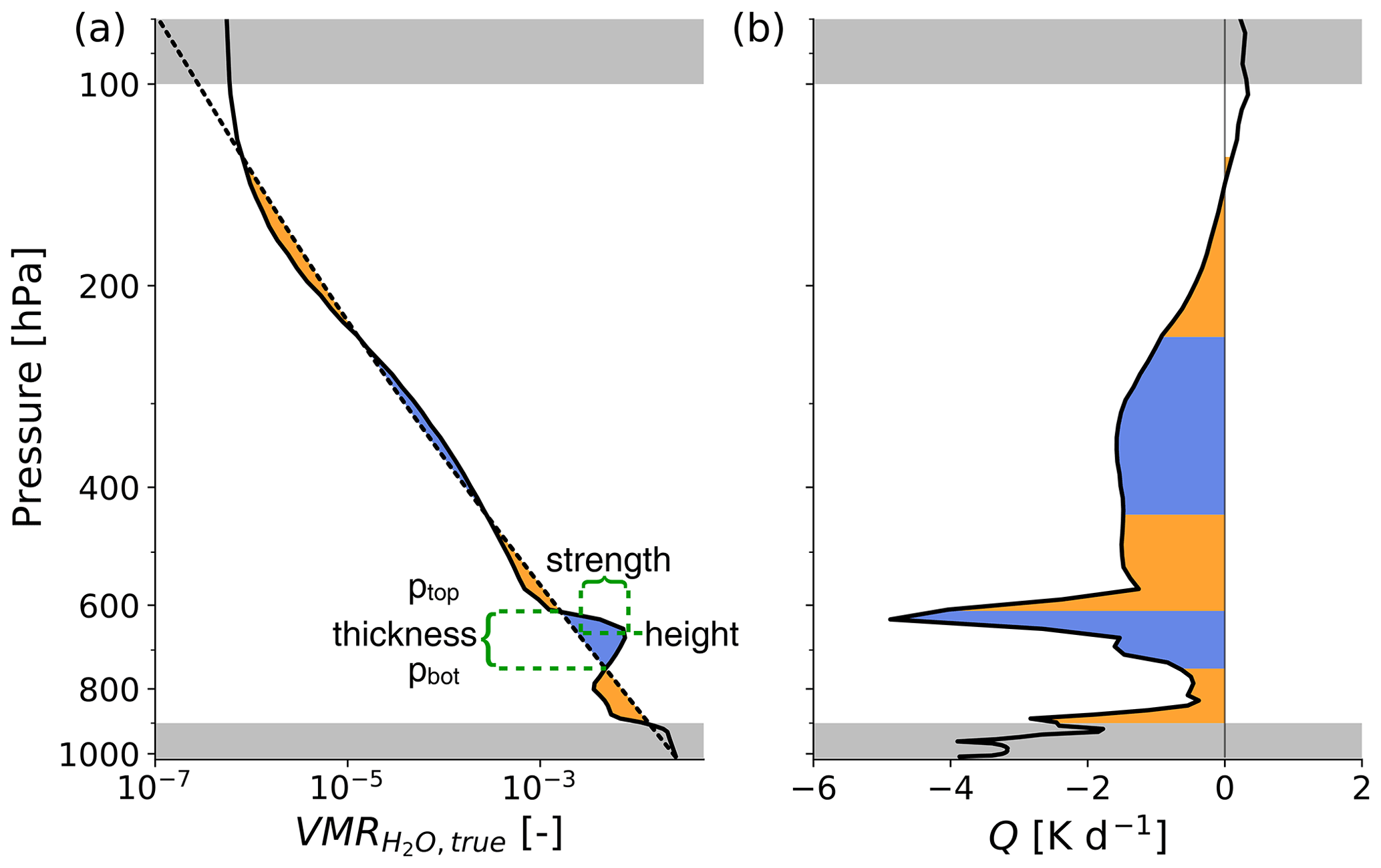
Figure 3Humidity profile (a) of an atmospheric case with a strong EML and the associated net heating rate (longwave + shortwave) profile (b). The reference humidity profile used to identify humidity anomalies is depicted as the dashed line in (a). Layers of moist anomalies are highlighted by blue shading, dry anomalies by orange shading. Anomalies that intersect with the grey-shaded regions are excluded to restrict anomalies to the free troposphere. The green lines and brackets conceptually display the definition of moisture anomaly characteristics from Table 1 for the strong positive anomaly at around 650 hPa.
Figure 3b shows the close relation between the vertical humidity structure and the net heating rate Q (longwave + shortwave), which is calculated with the radiative transfer model RRTMG (Rapid Radiative Transfer Model for GCMs, Mlawer et al., 1997) through its implementation in the radiative convective equilibrium model konrad (Kluft and Dacie, 2020). Q is calculated for all conducted retrievals throughout this study to assess whether the vertical humidity structure is captured in a way in which Q is also represented well.
Table 1Characterization metrics of moisture anomalies, their definitions and short descriptions. denotes the reference water vapour profile.
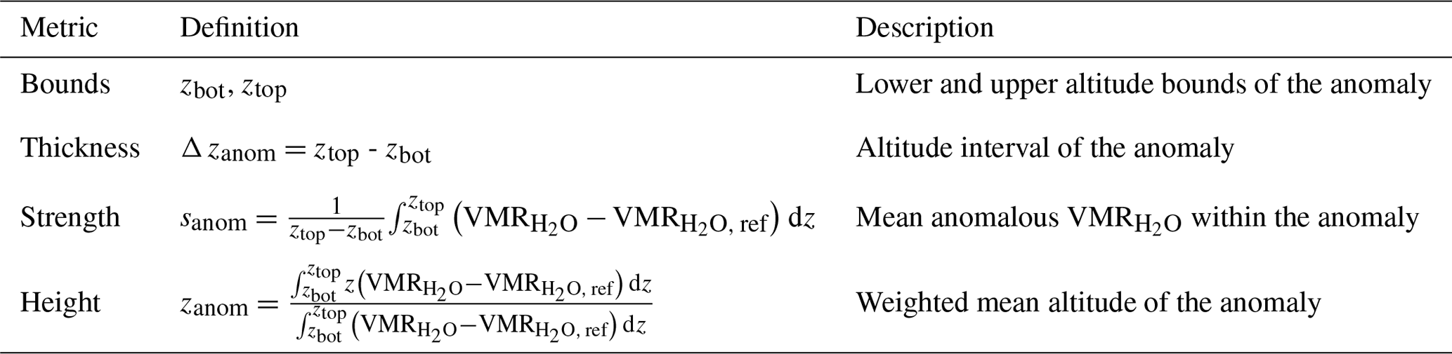
The blue and orange shadings associated with moist and dry anomalies depicted in Fig. 3 visualize that by definition layers of positive and negative moisture anomalies alternate in the vertical. Each such layer can be viewed as a moisture anomaly object, which we characterize by means of the scalar metrics introduced in Table 1. These metrics include the vertical bounds of the moisture anomaly in terms of altitude (zbot and ztop), the difference of which denotes the anomaly's thickness (Δ zanom). The anomaly height (zanom) is defined as the mean over the anomaly's height interval, weighted by the anomalous humidity within the altitude bounds. Finally, the anomaly strength (sanom) is defined as the mean anomalous within the anomaly's vertical bounds. We only consider positive (moist) anomalies that are fully captured in the pressure range between 100 and 900 hPa; e.g. the positive anomalies at the very top and bottom of Fig. 3 are neglected (grey shading) to avoid tropopause and boundary-layer-related anomalies.
In this section the retrieval introduced in Sect. 2 is applied to synthetic IASI observations of the dropsondes that sampled the EML discussed by Stevens et al. (2017). This case study is of particular interest because the found EML blind spot of Stevens et al. (2017) contradicts the results of other OEM-based studies discussed in Sect. 1.1. Here we first want to specifically assess the importance of temperature information for properly resolving the moisture structure in an EML scenario. While in general it is well known that the humidity retrieval depends on the quality of the assumed or retrieved temperature profile, we argue that for EMLs this effect is of particular relevance. In a next step, the averaging kernels for the EML scenario and a mean tropical ocean atmosphere are compared to estimate the retrieval's vertical resolution and its dependence on the atmospheric state.
4.1 Importance of temperature information for retrieving a moist layer
We assess the possibility of whether a lack of independent temperature information can cause the EML to not be resolved by running our retrieval in slightly altered setups. Each row of panels in Fig. 4 represents a variation of the retrieval. The setup introduced in Sect. 2 is used for the first row and serves as a basis for the other two setups. We refer to this setup as retrieval setup 1. Retrieval setup 2 (Fig. 4, second row) only deviates from retrieval setup 1 by using the narrower spectral region that was used by Lacour et al. (2012) and Stevens et al. (2017), which is limited to 1193 to 1223 and 1251 to 1253 cm−1. Retrieval setup 3 (Fig. 4, third row) only deviates from retrieval setup 2 by omission of the temperature retrieval and instead setting the a priori temperature to the true reference state. The profiles that the synthetic observations are based on are denoted as “true” and the same for all retrieval setups. Based on these profiles, forward-simulated synthetic IASI observations are calculated, synthetic Gaussian noise is added (see Sect. 2.5) and the retrieval is performed. As a technical note, we extrapolate the dropsonde profiles (launched at about 350 hPa) into the upper troposphere and above by fitting a tropical mean atmospheric state (Anderson et al., 1986). We fit these profiles onto a 137-level vertical pressure grid of the ECMWF IFS model atmospheres that also come with an associated altitude grid (Eresmaa and McNally, 2014).
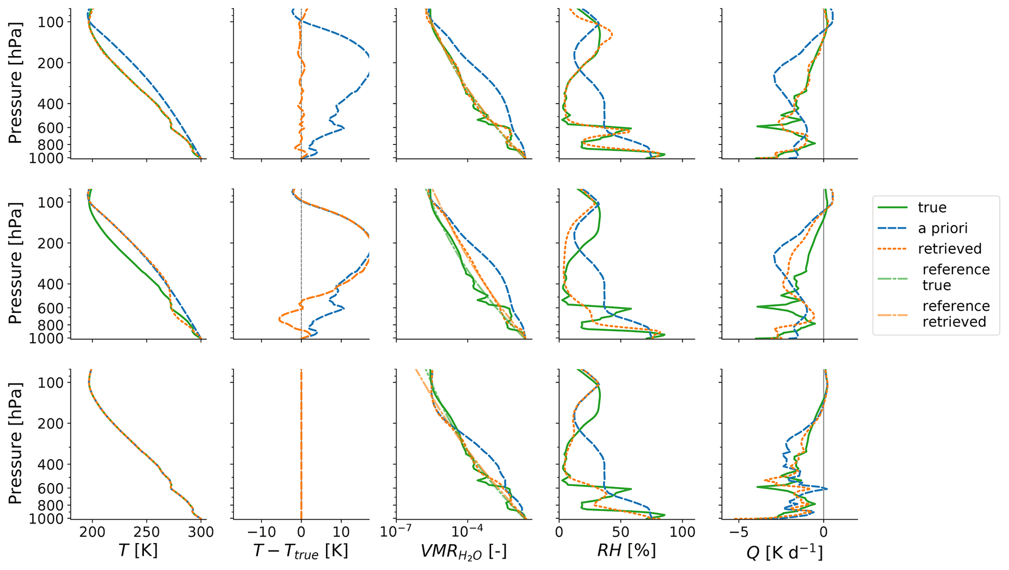
Figure 4Columns show profiles of temperature (T), temperature differences of a priori and retrieved states to the true state, , relative humidity (RH) and net heating rates (Q) for the dropsonde profiles that sampled the EML discussed by Stevens et al. (2017) (labelled as “true” here). Displayed are the true states that are used as a basis for the forward-modelled synthetic IASI observation, the a priori states of the retrieval and the retrieved states. The reference profiles defined in Sect. 3 are also depicted. Rows show retrieval results based on different retrieval setups that are introduced in the text.
As a note on comparability of our results to Stevens et al. (2017), we want to be cautious. There are several differences in the exact way the retrieval is set up, e.g. in the assumed a priori states and covariances, the iteration scheme (Gauss–Newton vs. LM) and also the radiative transfer model (Atmosphit vs. ARTS). Besides, our study is conducted in a synthetic framework, since we aim to assess the retrieval of EMLs more fundamentally than the discussed case studies did up to now. With this in mind, we tried to seek out a retrieval feature of the study of Stevens et al. (2017) that is capable of masking the EML in our setup. This feature is the used spectral region that is closely tied to the temperature information content, as we want to show in the following.
Looking at the retrieval results of Fig. 4, the EML structure is found to be resolved well with retrieval setup 1, while retrieval setup 2 misses the EML almost completely, comparable to the results of Stevens et al. (2017). We hypothesize that the missing EML with retrieval setup 2 is caused by the fact that with the limited spectral setup, there is no sufficient independent temperature information available for the retrieval to separate the moisture from the temperature signal, causing large retrieval errors in both quantities. While other previous retrieval studies deliberately try to account for this issue by deploying either a simultaneous retrieval approach (Smith et al., 2012; Weisz et al., 2013; Irion et al., 2018) or a sequential retrieval approach (Smith and Barnet, 2019, 2020; Susskind et al., 2014), we want to highlight the importance of doing so, specifically in an EML scenario.
We find that the large water vapour and temperature errors obtained with retrieval setup 2 around the EML altitude compensate radiatively. While the underestimated humidity at the EML altitude yields an increased spectral radiance in the used water vapour band due to a lower emission height associated with a higher emission temperature, the underestimated temperature yields a decreased spectral radiance. Since this compensation leads to comparatively low y costs in the OEM scheme, it explains why retrieval setup 2 finds an optimal solution that is associated with relatively large retrieval errors in both temperature and water vapour.
We introduce retrieval setup 3 to exclude the possibility that resolving the EML with retrieval setup 2 is simply limited by vertical resolution of the moisture retrieval, e.g. limited humidity information content. The retrieval results of retrieval setup 3 show that with a perfect prior temperature profile, the limited spectral range is also sufficient to resolve the general EML structure, albeit with reduced EML amplitude. Hence, the EML blind spot of retrieval setup 2 and possibly of Stevens et al. (2017) is a consequence of the ambiguity that lies in the limited spectral range with respect to temperature and water vapour.
Table 2Moisture anomaly characteristics of the EML shown in Fig. 4. This table is analogous to Table 1, where the exact definitions of the different metrics are explained. The EML characteristics displayed here are calculated for the true state and the retrieval results of retrieval setups 1 and 3, corresponding to upper and lower rows of Fig. 4, respectively. Retrieval setup 2 does not feature a moisture anomaly object as defined in Sect. 3.
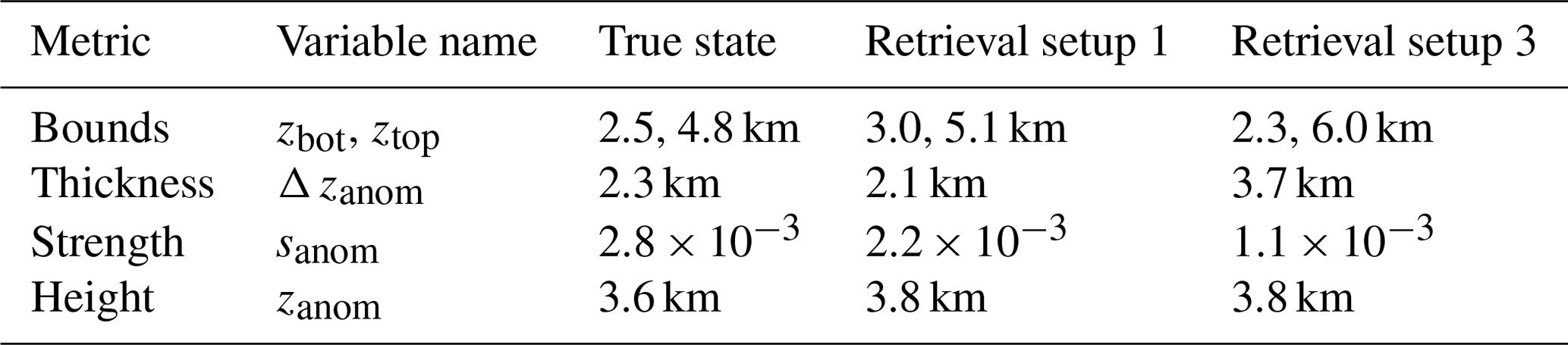
To exemplify the concept of the moisture anomaly identification and characterization method introduced in Sect. 3, we apply the procedure to this case study and present the derived EML characteristics for each of the different retrieval setups in Table 2. To identify the EML centred around 650 hPa in the true and retrieved profiles in Fig. 4, we introduce the respective reference profiles against which positive anomalies can be identified. While retrieval setups 1 and 3 yield a moisture anomaly that can be characterized by our method and compared to the characteristics of the true EML, retrieval setup 2 does not show a positive moisture anomaly around 650 hPa.
Table 2 shows that the EML in the true state is centred around 3.6 km altitude and has a vertical extent of 2.3 km. Retrieval setup 1 captures these characteristics reasonably well, while retrieval setup 3 shows a strongly overestimated EML thickness of about 3.7 km, reflecting stronger smoothing caused by the limited spectral range used in this setup. Both retrieval setups show a slightly increased EML height when compared to the true state of about 200 m for reasons we can only speculate on. We could see this being a systematic effect caused by a less pronounced effect of smoothing at the EML bottom due to higher optical density than aloft. Since the atmosphere is optically more dense near the surface, smoothing may smear the EML over a larger altitude interval at the top than at the bottom, positively biasing the EML altitude in the retrieval.
While the EML strength sanom may appear to be the least trivial moisture anomaly characteristic, being without units due to its definition based on , it becomes more intuitive when values are put into relation to each other. The true EML strength of , which reflects the mean anomalous within the EML, is about 30 % greater than the EML strength derived from retrieval setup 1 and about 2.5 times greater than the EML strength derived from retrieval setup 3. This reflects the notion that while retrieval setup 1 is able to resolve the EML well, retrieval setup 3 yields a strongly smoothed EML that is significantly less pronounced than its true counterpart.
We conclude that, while the EML investigated by Stevens et al. (2017) does not appear to be a general blind spot for hyperspectral IR satellite observations, we are able to find a retrieval configuration that reproduces a similar result to theirs. The deciding property of that configuration is the lack of independent temperature information, which in an EML scenario can yield radiatively compensating errors in temperature and water vapour. With retrieval setup 1, on the other hand, we present a retrieval setup that is able to capture both temperature and humidity profiles well, including the EML, which is in line with other OEM-based moist layer case studies (Zhou et al., 2009; Calbet et al., 2006).
4.2 Retrieval resolution
With OEM, a more quantitative estimation of vertical retrieval resolution can easily be deduced with the aid of the averaging kernel matrix A (Rodgers, 2000). The rows of A describe the response of the retrieved state to a perturbation in the true state, taking into account the specifications of the observing system. The averaging kernels presented here are based on the spectral setup and a priori assumptions introduced in Sect. 2.
Several previous studies showed IASI averaging kernels for mean atmospheric states (Lerner, 2002; Schneider and Hase, 2011; Smith and Weisz, 2018). Here we want to highlight the dependence of vertical resolution on the atmospheric state by contrasting the averaging kernels of a tropical mean atmosphere to the reference EML case discussed in the previous subsection. Smith and Barnet (2020) also considered the dependence of A on the atmospheric state, which they find can be quite severe. In contrast to their more general study, we want to focus on comparing the variability of A with respect to a well-characterized mean and EML state. While we focus on discussing the water vapour averaging kernels in this section, similar conclusions can be drawn about the temperature averaging kernels which are appended in Appendix A.
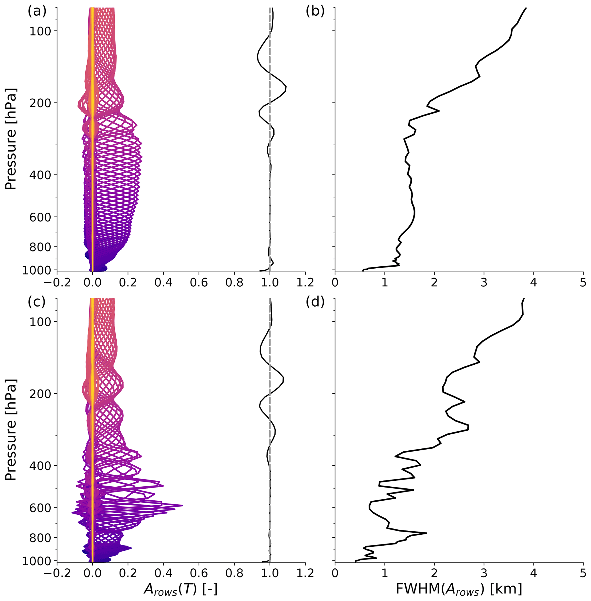
Figure 5a and c depict the rows of the H2O averaging kernel matrix as coloured lines for two different atmospheric setups. The more blue lines correspond to kernels closer to the surface, while the more yellow lines correspond to kernels higher up in the atmosphere. Figure 5a and b are based on an average tropical ocean atmosphere, namely the tropical FASCOD atmosphere introduced in Sect. 2.5. Figure 5c and d only differ in their base atmospheric state by the introduced EML, as described in Sect. 3. The vertical width of a kernel is a measure of the retrieval's vertical resolution at a specific height, which is shown in terms of the FWHM of the respective kernels in Fig. 5b and d. A measure of the retrieval's ability to detect and respond to a water vapour disturbance in the true state at a given height is the measurement response, which is defined as the sum over all kernel rows and depicted as the black line in Fig. 5a and c. Values close to unity indicate that the retrieval is sensitive to disturbances in the true profile (Rodgers, 2000).
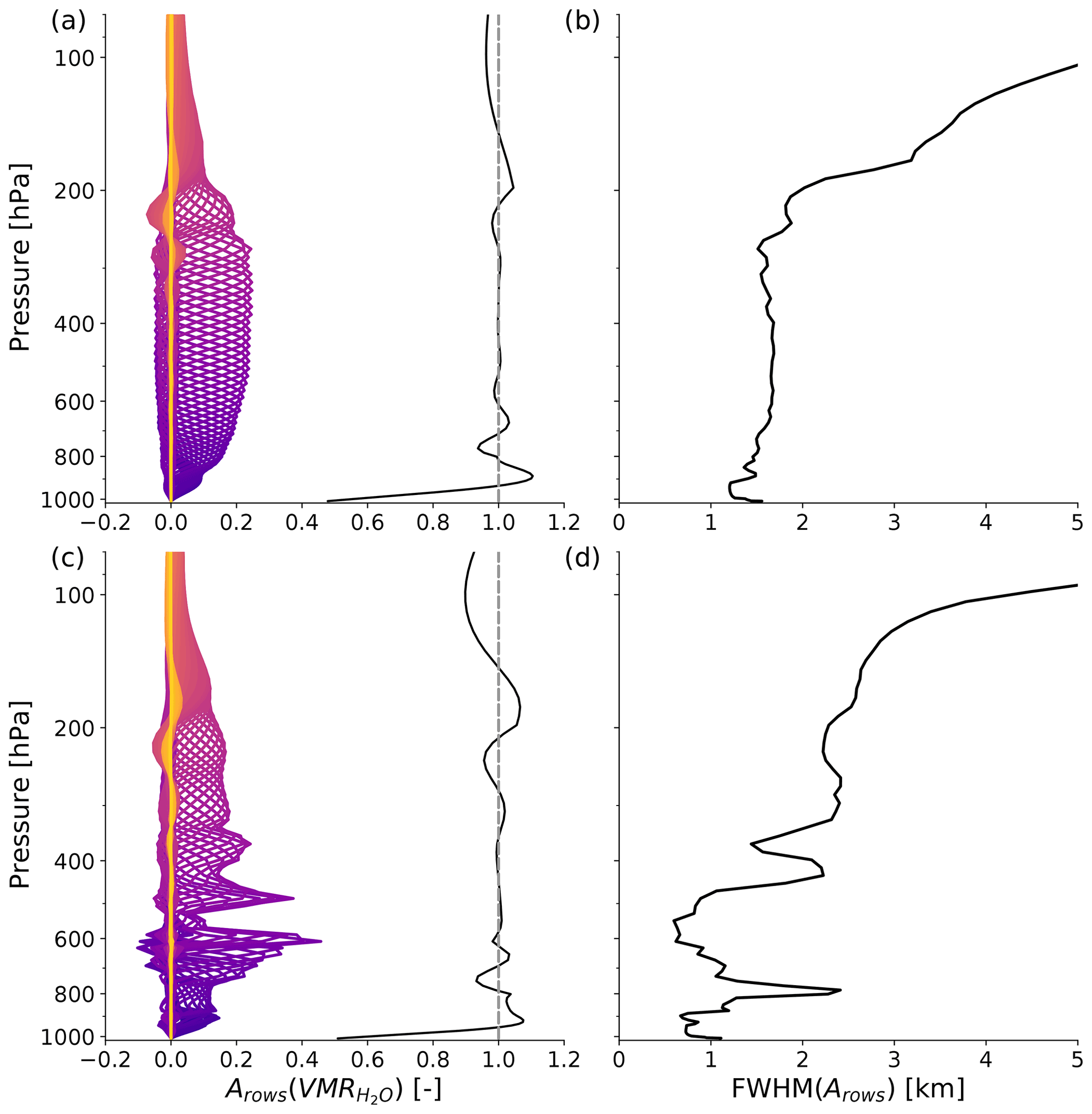
Figure 5Panels (a) and (c) show rows of the water vapour averaging kernel matrix () as coloured lines and their sum as a black line, which denotes the measurement response. The rather blue lines correspond to kernels closer to the surface, and the more yellow lines correspond to kernels at higher altitudes. Panels (b) and (d) show the FWHM of the averaging kernel rows, which is a measure for the vertical resolution of the observing system. Panels (a) and (b) are based on a mean tropical ocean atmosphere, specifically the tropical FASCOD atmosphere. The atmospheric setup used for (c) and (d) differs only by the introduction of EML features, as described in Sect. 3.
The averaging kernels of the mean tropical ocean atmosphere in Fig. 5a expectably show a very smooth behaviour with height, and the deduced vertical resolution is similar to that of Smith and Weisz (2018); e.g. it is of the order of 1.5 km throughout the free troposphere between around 200 and 800 hPa. In the upper troposphere (p≲200 hPa) a significant decrease in vertical resolution is found. In the boundary layer, the vertical resolution does not appear to diminish but to improve, which is in agreement with Smith and Weisz (2018). However, we find this to be misleading because the shape of the averaging kernels associated with these altitudes is distorted due to the strong signal of the surface, not allowing for a robust calculation of the FWHM. Rather than the FWHM, the measurement response is a more informative measure of the retrieval's sensitivity to disturbances in the boundary layer. For the tropical ocean atmosphere, the measurement response is close to unity throughout most of the free troposphere and shows a sharp decrease within the boundary layer, indicating limited sensitivity to water vapour disturbances in the true state only in the boundary layer.
The EML has a significant impact on all averaging kernels in the lower and mid troposphere as shown in Fig. 5c and d. Around the humidity maximum at the EML top the averaging kernels show distinct peaks, which are caused by the strong radiative signal associated with the EML. The EML signal is so strong that it also affects the more sensitive channels that usually sample higher altitudes and therefore decrease the vertical resolution from about 1.5 to 2.5 km between the EML top and about 200 hPa compared to the tropical mean atmosphere. As the moisture decreases beneath the EML humidity maximum, a clear reduction in vertical resolution down to about 2.5 km at around 800 hPa is found, indicating a more limited ability to resolve additional moisture features beneath the EML. This state dependence of the averaging kernel reflects the nonlinear nature of the retrieval problem and the limited expressiveness of the vertical resolution deduced with this method. Retrievability of a moisture feature not only depends on its vertical extent, but also on the atmospheric state it is embedded in. This motivates the statistical analysis presented in the next section of analysing the retrieval's performance with regard to its ability to capture moisture anomalies as introduced in Sect. 3.
After the exemplified investigation of an EML case in the previous section, the retrieval performance is now assessed based on a larger test dataset. The major aim with this section is to first assess the validity of our simple retrieval setup before using the synthetic retrieval dataset in the next section to showcase some of the possibilities with our new method for identifying and characterizing moisture anomalies introduced in Sect. 3. In the following, we first introduce the test dataset and investigate the vertical distribution of the retrieval error in temperature and water vapour. Afterwards, the smoothing error, which is an intrinsic source of error for a given observing system and a set of a priori assumptions, is calculated and discussed in the context of the overall retrieval error.
5.1 Reference dataset and retrieval error
The retrieval is applied to tropical ocean atmospheres (between 30∘ S and 30∘ N) that are part of the ECMWF IFS diverse profile database made available by Eresmaa and McNally (2014). The database consists of 25 000 short-range forecasts, which are divided into five even subsets that focus on representing diversity in a particular atmospheric quantity, such as temperature, specific humidity or precipitation. For the purpose of this work, only the tropical ocean atmospheres of the subset that focuses on a diverse sampling of specific humidity is considered. This yields a total number of 1599 atmospheric setups, for 1288 of which the retrieval converges to a solution. The following analysis is based on these converged cases.

Figure 6Panels (a), (b) and (c) give a statistical overview of temperature, and RH over 1288 tropical ocean model atmospheres from the dataset of Eresmaa and McNally (2014), upon which the retrieval is performed. Colour scheming is based on Fig. 5 of Eresmaa and McNally (2014), where bright orange indicates the 10th and 90th percentiles and dark orange indicates the 25th and 75th percentiles. The median is depicted by a solid black line. Panels (e), (f) and (g) show the respective statistics on the deviations of the retrieved to true profiles. Note the exception of relative differences for , which is more suited for the dynamical range of this quantity.
A statistical overview of the variability of temperature and humidity profiles covered by the tropical ocean dataset is provided in Fig. 6a, b and c. The temperature profiles show very limited variability, as is typical for tropical ocean regions. However, despite this very smooth appearance of the vertical temperature structure, the individual profiles do include significant temperature inversions, for example the very prominent inversion at about 2 km height in the trade wind region (not shown). The humidity profiles show weak variability within the boundary layer, where the ocean acts as a humidity source and humidity is mostly set by the saturation vapour pressure controlled by temperature. The median RH is about 82 % at the surface and reaches its maximum at about 500 m height in the transition to the shallow cloud layer. In the free troposphere, the typical “C”-shaped structure of the RH profile is followed (Romps, 2014). An interesting feature in the 75th and 90th percentiles of the RH profiles is the presence of positive RH anomalies in the layer between around 500 and 700 hPa, indicating moisture anomalies that may be tied to the freezing level.
Figure 6d, e and f show an overview of the retrieval's deviations from the reference dataset, from now on referred to as the retrieval error. In the context of these figures, the term bias refers to a difference of the median values of the retrieved and true datasets. The temperature profile shows a positive bias close to the surface, which we attribute to the limited signal from these heights in the satellite observation. The negative bias near the surface in RH is associated with this positive temperature bias and with the slightly negative bias near the surface. Between around 900 and 700 hPa the and RH biases are positive, while the temperature bias is slightly negative. This positive moisture bias in the lower troposphere is associated with an increased variability of the error, particularly towards strong positive errors that indicate an overestimation of moisture in the lower troposphere by the retrieval. This may be caused by the typical hydrolapse that is coupled to the trade inversion in the trade wind regions, which can in its sharpness not be captured by the retrieval.
In the mid troposphere between about 700 and 300 hPa, which is where typical EMLs are expected, no significant temperature or humidity biases are found. A positive skewness in the error distribution towards strong positive errors is found, indicating that positive errors in retrieved are rare but large compared to the negative errors that occur. As an explanation for this error pattern, we propose the idea that positive (moist) moisture anomalies tend to be captured with a slight underestimation in their strength, while occasionally strong negative (dry) moisture anomalies beneath are associated with a strong overestimation of moisture by the retrieval due to a lack of signal beneath a positive moisture anomaly (as shown in Fig. 5). This could explain less frequent but strong positive retrieval errors and more frequent but relatively weak negative errors that have a net bias close to zero.
In the upper troposphere errors in temperature and humidity are generally larger. We believe that this has two causes. Firstly, the a priori moist adiabatic temperature assumption becomes worse closer to the tropopause. Secondly, Fig. 5 shows that there is only a weak radiative signal from the upper troposphere, as indicated by strongly smoothed averaging kernels and a decreased vertical resolution. While this may be improved by adjusting the a priori assumptions for the upper troposphere and including even stronger absorption features of water vapour, the upper troposphere is no major concern of this study.
5.2 Smoothing error
Part of the retrieval error shown in Fig. 6 can be attributed to the so-called smoothing error (SE, Rodgers, 2000). Given a specific observing system and a priori assumptions about the quantity to be observed, the SE is a source of error that cannot be avoided without changing the observing system or a priori assumptions themselves. In the framework of the averaging kernel matrix, the SE expresses the error in the retrieval that is associated with the non-delta-function shape of the averaging kernel rows (see Fig. 5) and the thereby limited ability to resolve vertical features. Here, it is calculated as
where In denotes the identity matrix of order n and n is the number of vertical levels of the profile retrieval.
Figure 7 shows the SE statistics associated with the retrieved temperature and humidity profiles of the tropical ocean dataset. The median of the SE with respect to the temperature profile (SE(T)) is close to zero throughout most of the free troposphere, similar to the retrieval bias shown in Fig. 6d. The positive retrieval bias in temperature found near the surface is of smaller magnitude also found in SE(T), indicating that this pattern is caused by a systematically unresolved vertical feature. The variability of the temperature retrieval error found in Fig. 6d in the lower and mid troposphere cannot be attributed to smoothing, since the variability in SE(T) is very small. In conclusion, this indicates that temperature error sources are unlikely to be caused by uncaptured vertical temperature variability but rather vertically constant errors, which do not show up in SE(T). In the upper troposphere, SE(T) increases towards the tropopause, where smoothing becomes the major contribution to the retrieval temperature error.
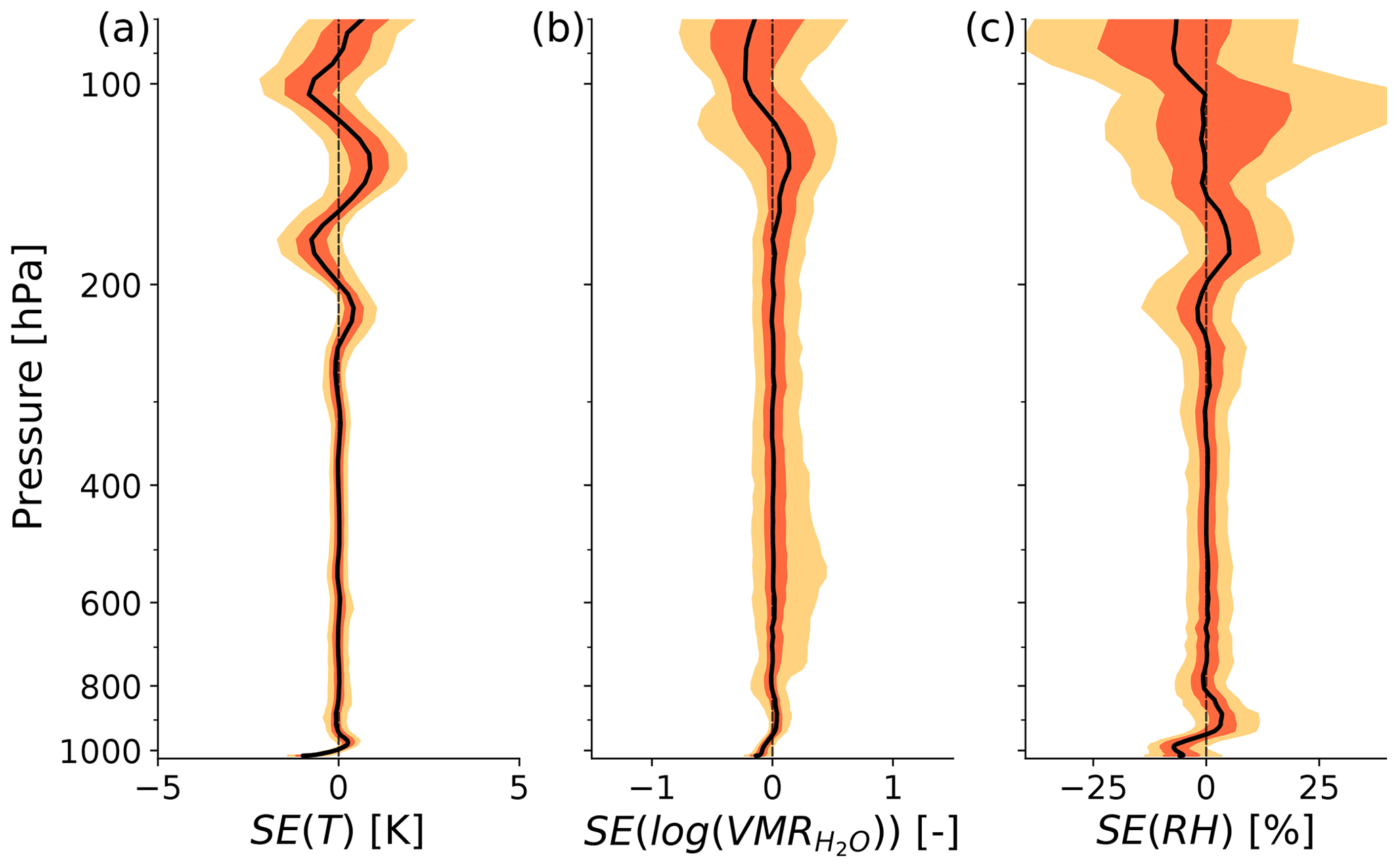
For the water vapour profile in the lower and mid troposphere, smoothing is a greater source of error than for the temperature profile (Fig. 7b). While the median of the water vapour smoothing error () is low throughout the lower and mid troposphere, its variability (e.g. the shown percentile ranges) is on a similar scale to the variability of the retrieval error shown in Fig. 6e. This indicates that a major contribution of error in the water vapour retrieval is to capture vertical variability. The distribution of in the mid troposphere also reflects the positive skewness that was found in the overall error in Fig. 6e. This is consistent with the previously described idea that this skewness is linked to the retrieval's ability to capture vertical moisture anomalies. In the upper troposphere, the median increases to a similar magnitude to the retrieval error, while its variability even exceeds that of the retrieval error, indicating that other sources of error are compensating.
The SE(RH) statistics show the combined effect of the smoothing errors in temperature and humidity (Fig. 7c). It is apparent that also in terms of RH the smoothing error has a strong contribution to the retrieval error in the lower and mid troposphere, similar to the error. In the upper troposphere the median SE(RH) is of the same order as the retrieval error, while its variability appears to be even stronger, following the behaviour found for .
In this section the retrieval results for the previously introduced tropical ocean test dataset (Sect. 5) are assessed with specific focus on the characteristics of moisture anomalies as introduced in Sect. 3. First, the moisture anomaly characteristics of the tropical ocean dataset and of the retrieved dataset are compared to look for systematic limitations of the retrieval to resolve specific kinds of moisture anomalies. Then, the impact of moisture anomalies on the heating rate profile is assessed and the retrieval's ability to capture this impact is investigated.
6.1 Moisture anomaly characteristics
Figure 8 shows probability density distributions of the moisture anomaly characteristics (defined in Sect. 3) for the tropical ocean dataset (green) and the associated retrieved dataset (orange). The dashed lines indicate the mean values of the respective distributions. The distributions of moisture anomaly height (zanom) displayed in Fig. 8a show that most moisture anomalies occur in the mid to upper troposphere, which is somewhat surprising since EMLs are typically thought to be coupled to the freezing level at around 5 km height (Johnson et al., 1996; Stevens et al., 2017). However, note firstly that strong EMLs and very slight moisture anomalies are treated evenly here. Secondly, the distributions reflect the statistics of the underlying dataset, which is based on the ECMWF IFS atmospheric model. This dataset appears as a suitable starting point to assess the retrieval's ability to capture moisture anomalies; however, the analyses of the dataset's moisture anomaly statistics themselves are not the focus of this study.
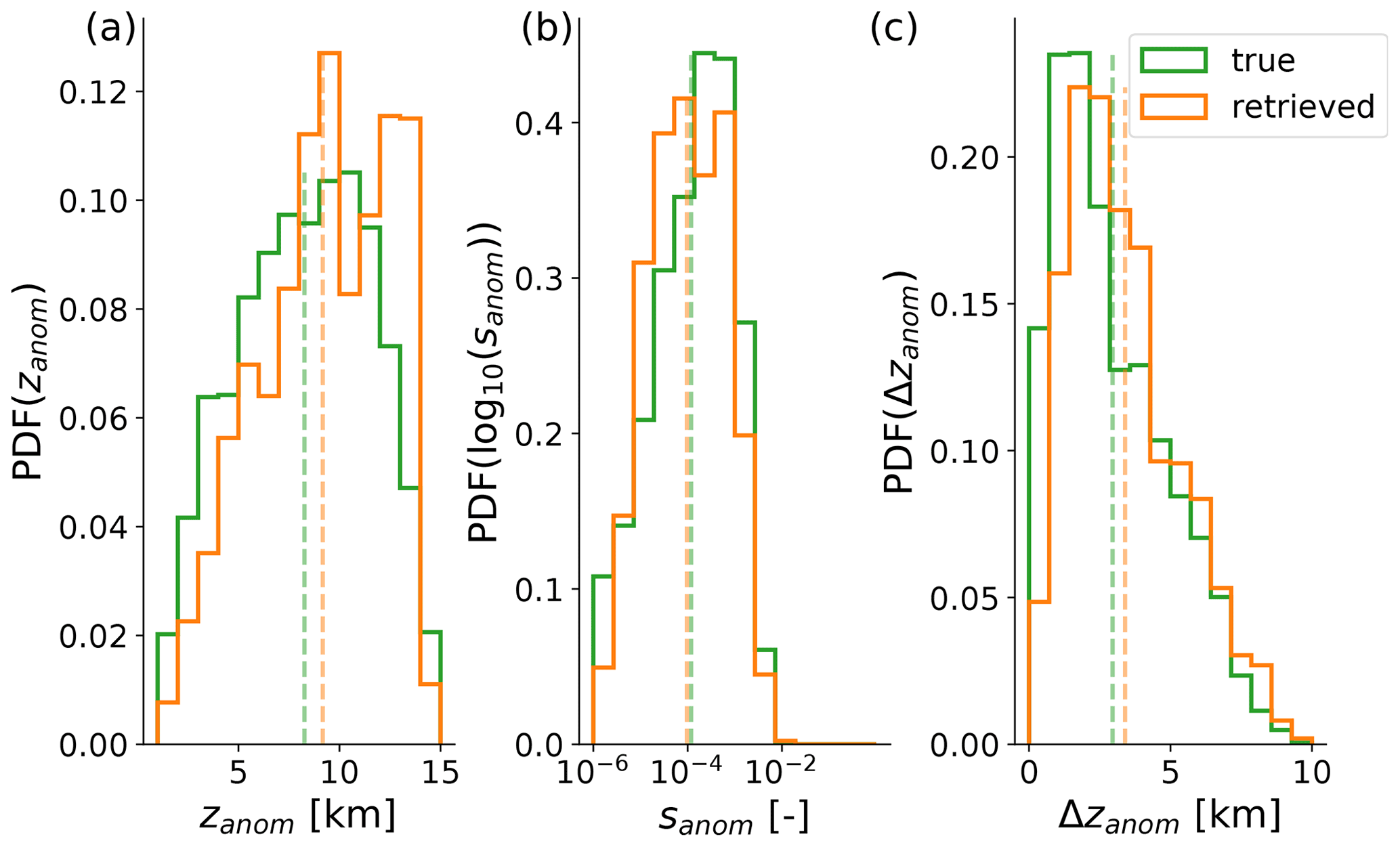
Figure 8Probability density functions (PDFs) of moisture anomaly characteristics of the tropical ocean reference dataset (denoted as “true”) and the retrieved dataset.
Figure 8a shows a bias between true and retrieved zanom of about 0.9 km, indicating that the found zanom biases in the case study of Sect. 4 do indeed appear to be systematic and even greater in amplitude. Besides the earlier proposed cause of a varying effect of smoothing with height, we believe this bias is also caused by a systematic underestimation of the fraction of moisture anomalies below 5 km altitude by the retrieval, while the fraction of anomalies above 10 km is overestimated. Only a fraction of about 52 % of the total number of moisture anomalies below 5 km in the reference dataset is captured by the retrieval. We attribute this deficiency to the fact that moisture anomalies are typically narrower in the lower to mid troposphere than further aloft, as shown in Fig. 9.
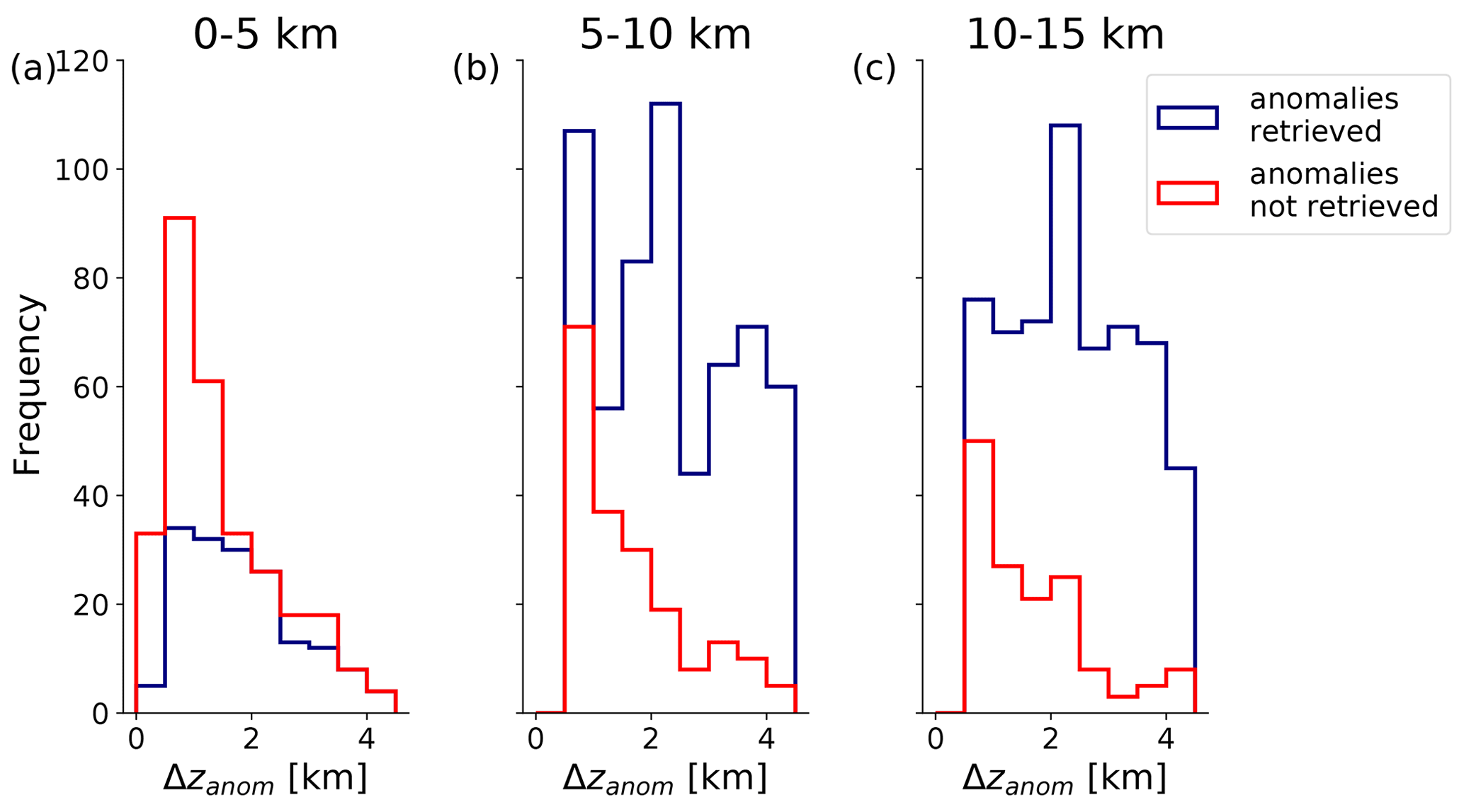
Figure 9Frequency distributions of moisture anomaly thickness of the tropical ocean reference dataset, split up into cases where a moisture anomaly could be retrieved and could not be retrieved. Panels (a), (b) and (c) reflect three altitude regions, namely the lower (0–5 km), mid (5–10 km) and upper (10–15 km) troposphere.
Figure 9a, b and c show the number of moisture anomalies of the reference dataset in the lower, mid and upper troposphere, respectively, as a function of anomaly width (Δ zanom) and separated into subsets of anomalies that either could or could not be retrieved. An anomaly of the reference dataset is considered retrieved if there is a retrieved positive moisture anomaly with an anomaly height within the vertical bounds of the anomaly of the reference dataset. While it is apparent that the narrower moisture anomalies are most frequently missed in all three altitude regions, this means a particular shortcoming for the retrieval between 0 and 5 km because cases with Δ zanom≳2 km are especially rare. A technical cause of this is the fact that we exclude all anomalies that reach as close to the surface as 900 hPa (see Sect. 3). However, the lower to mid troposphere is also subject to more small-scale variability due to its link to the boundary layer and low-level convection, making it more prone to small-scale moisture anomalies than the free troposphere aloft.
The distribution of the moisture anomaly strength (sanom) depicted in Fig. 8b has a similar dynamical range to since the anomalous scales with its absolute value. The distribution of sanom of the retrieved dataset is overall shifted towards lower values, yielding a negative bias of about (17 %) against the reference dataset, which can mostly be attributed to the smoothing error of the retrieval. The smoothing error generally acts by a weakening and thickening of anomalies, which also partly explains the significant positive bias of about 0.4 km (15 %) in moisture anomaly thickness (Δ zanom) depicted in Fig. 8c. Another contributing effect towards the found biases in sanom and Δ zanom is the fact that particularly weak and narrow moisture anomalies are more often completely missed by the retrieval, as shown by Fig. 9.
6.2 Implications of moisture anomalies for the heating rate profile
Moisture anomalies affect the heating rate profile by absorbing and emitting IR radiation. Because of the exponential decrease in water vapour with height, emission at the anomaly top is particularly efficient and can yield a strong local radiative cooling rate (see Fig. 3). We consider this cooling effect to be the moisture anomaly's most prominent footprint on the heating rate profile. In the following, we quantify this cooling effect by considering the minimum heating rate within the vertical bounds of a moisture anomaly, min(Qanom). Since min(Qanom) is a scalar metric, it can intuitively be viewed as a function of moisture anomaly characteristics.
Figure 10a and b show the joint frequency distributions of the moisture anomaly strength (sanom) and min(Qanom) for the tropical ocean dataset and the retrieval dataset, respectively. Both datasets show a clear correlation between the two quantities, namely that stronger anomalies are associated with a stronger peak in radiative cooling. While moisture anomalies with sanom≲10−4 show similar minimum cooling rates down to about −2.5 K d−1 in both the reference and retrieval datasets, larger differences between the two datasets are apparent for stronger anomalies. The reference dataset (Fig. 10a) shows min(Qanom) values between about −1 and −5 K d−1 for moisture anomalies with sanom≳10−4, while the retrieval dataset barely shows any min(Qanom) values smaller than −3 K d−1.
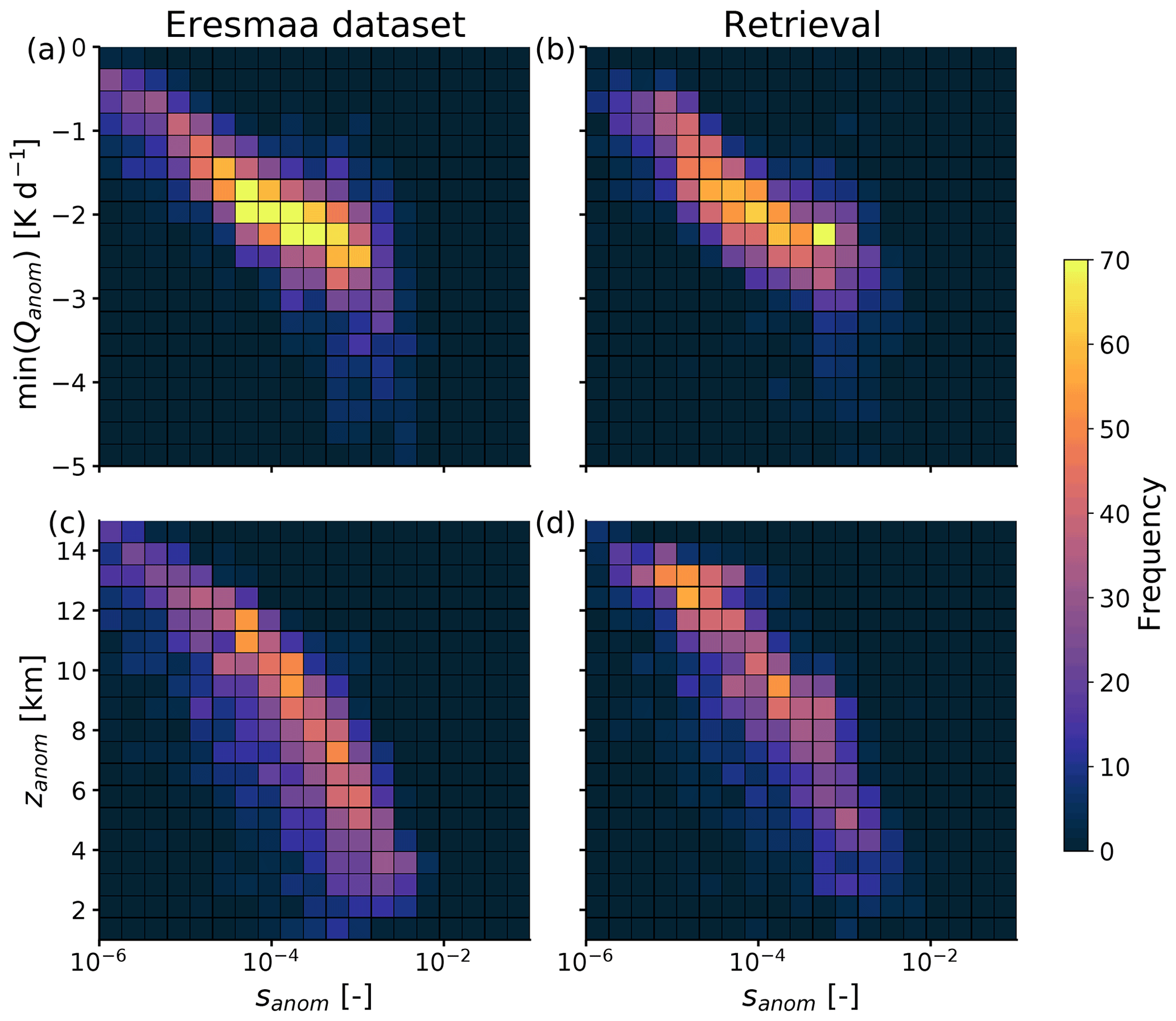
Figure 10Panels (a) and (b) show the joint frequency distributions of anomaly strength and minimum heating rate within the anomaly layers of the reference dataset and the retrieved dataset, respectively. Panels (c) and (d) show the joint frequency distributions of the anomaly strength and the anomaly height for the two respective datasets.
We hypothesize that the increased variability in min(Qanom) for sanom≳10−4 in the reference dataset can be attributed to the variability in the exact vertical shapes of the moisture anomalies. Anomalies with a strong negative moisture gradient at their top yield a stronger minimum in radiative cooling, while more smooth anomalies are associated with a less pronounced radiative cooling peak. This effect introduces more variability in min(Qanom) the stronger the anomalies are. It also explains why retrieved moisture anomalies do not show as extreme min(Qanom) values as the reference dataset, since the vertical shape of retrieved anomalies is always bound by the smoothing error.
In the real world, much more extreme vertical moisture gradients associated with moisture anomalies can be observed than in the model-based reference dataset used here. Albright et al. (2021) discuss an EML scenario over the Northern Atlantic Trades with a significant moisture drop that is associated with a minimum cooling rate of about 20 K d−1. The results of Fig. 10 indicate that while the retrieval is able to broadly distinguish between differently strong moisture anomalies and their associated heating rates, it is unable to properly represent such extreme cooling rate minima due to smoothing.
Figure 10c and d show the joint frequency distributions of the moisture anomaly strength and height (zanom). A clear relation between sanom and zanom is found in both datasets, namely that anomalies are weaker the higher up they are in the troposphere. We explain this by the dependence of sanom on the absolute humidity, which decreases exponentially with height. Combining this with the relation found between anomaly strength and minimum heating rate, it is clear that the radiatively most significant moisture anomalies occur in the lower to mid troposphere. As pointed out in Sect. 6.1 when discussing Fig. 9, the retrieval has particular deficiencies in resolving the rather narrow lower- to mid-tropospheric moisture anomalies. It is now apparent that this deficiency is particularly relevant, since it affects the strongest and radiatively most significant moisture anomalies. However, the EML test case investigated in Sect. 4.1 shows that when the anomaly is relatively strong and the atmosphere aloft has a simple structure, lower- to mid-tropospheric moisture anomalies can also be retrieved well. It may be worth investigating different cases of EMLs that are embedded in a more complex tropospheric humidity structure in the future.
The question implicitly raised by the findings of Stevens et al. (2017), whether or not passive satellite retrievals are capable of resolving EMLs, is investigated based on a synthetic retrieval framework where the IASI instrument is represented by the forward model ARTS. An EML test case based on dropsonde profiles from the NARVAL-2 measurement campaign (Konow et al., 2019) and a set of 1288 tropical ocean model atmospheres are used as input for the forward model and as a reference to evaluate the retrieval results against. The scenes are limited to clear sky.
To characterize an EML quantitatively (e.g. by strength, thickness and height), the concept of a moisture anomaly against a loosely fitted but clearly defined reference humidity profile is introduced. Following the ideas of Johnson et al. (1996) and Stevens et al. (2017) about a coupling of EMLs to the freezing level, EMLs would in this framework constitute a subset of rather strong, vertically confined, lower- to mid-tropospheric positive moisture anomalies. However, for the scope of this work no clear specification of what distinguishes an EML from other moisture anomalies is attempted, which would require a more dedicated selection and analysis of the test dataset. Instead, the aim of this study is a first systematic evaluation of EML retrievability based on hyperspectral IR observations.
Based on the EML case of Stevens et al. (2017), we show that with sufficient independent temperature and water vapour information, a combined retrieval of the moisture and temperature profiles and the surface temperature is capable of resolving the vertical EML structure. This result is in line with previous OEM-based case studies of similar moisture structures (Calbet et al., 2006; Zhou et al., 2009). We show that limited independent temperature information can cause the EML to not be resolved by the retrieval due to compensating water vapour and temperature errors. We suggest this as a possible reason for the EML blind spot found by Stevens et al. (2017).
The EML signal for the IASI instrument is further characterized by the averaging kernel and the deduced vertical resolution, which is of the order of 1.5 km for an average tropical ocean atmosphere, which is in agreement with previous studies (Lerner, 2002; Smith and Weisz, 2018). However, in the presence of an EML, the strong signal from the EML top weakens the signal from below and introduces a strong gradient in vertical resolution from 0.5 km at the EML top to 2.5 km at the EML bottom. This state dependence of vertical resolution motivates a statistical approach to evaluate the retrieval's ability to resolve moisture anomalies in various atmospheric states.
When applying the retrieval to the tropical ocean test dataset, it is found that a large fraction of the absolute retrieval error in humidity can be attributed to smoothing. In particular, in the transition region between the boundary layer and the free troposphere, the smoothing error introduces a bias to the retrieved humidity and temperature profiles, which is most likely connected to the sharp humidity drop associated with the stratified barrier between the moist boundary layer and the dry free troposphere in the trade wind region. In the free troposphere, say above 800 hPa, the retrieval shows no significant moisture bias but a positively skewed error variability, indicating that moist anomalies are typically associated with smaller errors than dry anomalies. This is coherent with the idea that dry anomalies that occur beneath moist anomalies are prone to larger errors due to the reduced sensitivity of the satellite measurement below a moist anomaly.
The study is completed by a specific evaluation of the moisture anomaly retrievability based on the new characterization method introduced in Sect. 3. It is found that the retrieved moisture anomalies are on average 17 % weaker and 15 % thicker than the anomalies of the reference dataset, which we attribute to smoothing and the fact that rather weak and narrow anomalies are missed by the retrieval more often. While overall about 80 % of the total number of moisture anomalies in the reference dataset are found by the retrieval, a systematic underrepresentation of anomalies below 5 km is found, where the retrieval only identifies about 52 % of the anomalies present in the reference dataset. Since it is shown that moisture anomalies in the lower to mid troposphere are typically the strongest and radiatively most significant, this issue may be quite significant.
The analysis of capturing the moisture anomalies' footprint on the heating rate profiles shows that the retrieval is able to capture the general relation between anomaly strength and minimum cooling rate. However, the retrieval shows a particular shortcoming in capturing the most extreme cooling rates associated with strong lower- to mid-tropospheric anomalies. We attribute this shortcoming to the retrieval's limited ability to resolve strong vertical moisture gradients that are necessary for the most extreme local cooling rates. Vertical moisture gradients in the real world can be a lot stronger than the ones available from the model test dataset (Albright et al., 2021), which means that retrieval errors with respect to peaks in the cooling rates can be large for rather extreme but realistic cases.
In summary, the retrieval result of the EML case study shows that hyperspectral IR satellite instruments are in principle capable of resolving a sufficiently strong EML in an otherwise simply structured atmospheric profile. The statistical evaluation of retrieved moisture anomaly characteristics shows that the retrieval is able to represent moisture anomalies of various thickness, height and strength. Significant shortcomings are found in the lower to mid troposphere, where about half of the moisture anomalies are missed by the retrieval and with regard to capturing particularly strong vertical gradients, causing limitations in resolving extreme cooling rates. It would be interesting to apply a similar analysis to operational retrieval products, such as the IASI L2 product (EUMETSAT, 2017), the NUCAPS product (NOAA Unique Combined Atmospheric Processing System; Berndt et al., 2020) or the CLIMCAPS product (Community Long-term Infrared Microwave Combined Atmospheric Product System; Smith and Barnet, 2020). The benefit of our new method for analysing moisture anomalies is that it allows for a direct statistical evaluation of the different product's capabilities to resolve EMLs and vertical humidity structures in general by being easy to apply to large datasets. As a next step we plan to apply our retrieval and evaluation techniques introduced in this work to real hyperspectral IR observations, with a focus on EML-like cases that we identify based on dropsonde observations from the NARVAL and EUREC4A (Stevens et al., 2021) measurement campaigns. This may also serve as a good first test bed of data to assess operational products' capabilities to resolve the vertical moisture structures of interest.
The code for the radiative transfer model ARTS, which also includes the module that was used to conduct the OEM retrieval, is described by Buehler et al. (2018) and is freely available at https://github.com/atmtools/arts (ARTS developers, 2021).
The atmospheric profiles over tropical oceans that were used as a basis for the forward-modelled IASI spectra and the spectra themselves are publicly available on Zenodo (https://doi.org/10.5281/zenodo.4501184, Prange et al., 2021). The atmospheric profiles are a subset of the ECMWF IFS diverse profile database published by Eresmaa and McNally (2014) and is available on the NWP SAF website (https://nwp-saf.eumetsat.int/site/software/atmospheric-profile-data/, last access: 21 October 2021).
MP conducted the radiative transfer and the retrieval calculations and prepared the manuscript. MB and SAB supervised the analysis of the retrieval results, contributed ideas to the manuscript and revised it.
The authors declare that they have no conflict of interest.
Publisher’s note: Copernicus Publications remains neutral with regard to jurisdictional claims in published maps and institutional affiliations.
The authors would like to thank Simon Pfreundschuh, currently at Chalmers University of Technology, for his guidance on the OEM functionality of ARTS. The authors would like to thank Lukas Kluft, currently at the Max Planck Institute for Meteorology in Hamburg, for his guidance on the calculation of heating rates with konrad and for helpful discussions along with Theresa Lang, currently at Universität Hamburg (University of Hamburg). Finally, our thanks go to the ARTS radiative transfer community for their help with using ARTS.
This work is a contribution to the DFG-funded Cluster of Excellence “CLICCS – Climate, Climatic Change, and Society” (EXC 2037, project number 390683824) and to the Center for Earth System Research and Sustainability (CEN) of Universität Hamburg.
This work was funded by the German Research Foundation (DFG) in project “Elevated Moist Layers – Using HALO during EUREC4A to explore a blind spot in the global satellite observing system”, project BU 2253/9-1, part of DFG priority programme HALO SPP 1294, project number 316646266.
This paper was edited by Brian Kahn and reviewed by three anonymous referees.
Albright, A. L., Fildier, B., Touzé-Peiffer, L., Pincus, R., Vial, J., and Muller, C.: Atmospheric radiative profiles during EUREC4A, Earth Syst. Sci. Data, 13, 617–630, https://doi.org/10.5194/essd-13-617-2021, 2021. a, b, c
Ananthakrishnan, R. and Kesavamurthy, R. N.: Some new features of the vertical distribution of temperature and humidity over Bombay, during the south-west monsoon season, J. Mar. Biol. Assoc. India, 14, 732–742, available at: http://mbai.org.in/php/journaldload.php?id=681&bkid=45 (last access: 21 October 2021), 1972. a
Anderson, G., Clough, S., Kneizys, F., Chetwynd, J., and Shettle, E.: AFGL Atmospheric Constituent Profiles (0.120 km), AFGL-TR, 86-0110, Environmental research papers, Hanscom AFB, Mass., USA, no. 954, 1986. a, b
ARTS developers: The Atmospheric Radiative Transfer Simulator, Version: 2.5.0, GitHub [code], available at: https://github.com/atmtools/arts, last access: 21 October 2021. a
Berndt, E., Smith, N., Burks, J., White, K., Esmaili, R., Kuciauskas, A., Duran, E., Allen, R., LaFontaine, F., and Szkodzinski, J.: Gridded Satellite Sounding Retrievals in Operational Weather Forecasting: Product Description and Emerging Applications, Remote Sens., 12, 3311, https://doi.org/10.3390/rs12203311, 2020. a, b
Bony, S., Stevens, B., Frierson, D. M. W., Jakob, C., Kageyama, M., Pincus, R., Shepherd, T. G., Sherwood, S. C., Siebesma, A. P., Sobel, A. H., Watanabe, M., and Webb, M. J.: Clouds, circulation and climate sensitivity, Nat. Geosci., 8, 261–268, https://doi.org/10.1038/ngeo2398, 2015. a
Borger, C., Schneider, M., Ertl, B., Hase, F., García, O. E., Sommer, M., Höpfner, M., Tjemkes, S. A., and Calbet, X.: Evaluation of MUSICA IASI tropospheric water vapour profiles using theoretical error assessments and comparisons to GRUAN Vaisala RS92 measurements, Atmos. Meas. Tech., 11, 4981–5006, https://doi.org/10.5194/amt-11-4981-2018, 2018. a
Boukachaba, N., Guidard, V., and Fourrié, N.: Land surface temperature retrieval from IASI for assimilation over the AROME-France domain, EUMETSAT Meteorological Satellite Conference, 21–25 September 2015, Toulouse, France, 2015. a
Buehler, S. A., Mendrok, J., Eriksson, P., Perrin, A., Larsson, R., and Lemke, O.: ARTS, the Atmospheric Radiative Transfer Simulator – version 2.2, the planetary toolbox edition, Geosci. Model Dev., 11, 1537–1556, https://doi.org/10.5194/gmd-11-1537-2018, 2018. a, b
Calbet, X., Schlüssel, P., Hultberg, T., Phillips, P., and August, T.: Validation of the operational IASI level 2 processor using AIRS and ECMWF data, Adv. Space Res., 37, 2299–2305, https://doi.org/10.1016/j.asr.2005.07.057, 2006. a, b, c, d
Cao, G., Giambelluca, T. W., Stevens, D. E., and Schroeder, T. A.: Inversion Variability in the Hawaiian Trade Wind Regime, J. Climate, 20, 1145–1160, https://doi.org/10.1175/JCLI4033.1, 2007. a
Chang, S., Sheng, Z., Du, H., Ge, W., and Zhang, W.: A channel selection method for hyperspectral atmospheric infrared sounders based on layering, Atmos. Meas. Tech., 13, 629–644, https://doi.org/10.5194/amt-13-629-2020, 2020. a
Chazette, P., Marnas, F., Totems, J., and Shang, X.: Comparison of IASI water vapor retrieval with H2O-Raman lidar in the framework of the Mediterranean HyMeX and ChArMEx programs, Atmos. Chem. Phys., 14, 9583–9596, https://doi.org/10.5194/acp-14-9583-2014, 2014. a, b
Clerbaux, C., Boynard, A., Clarisse, L., George, M., Hadji-Lazaro, J., Herbin, H., Hurtmans, D., Pommier, M., Razavi, A., Turquety, S., Wespes, C., and Coheur, P.-F.: Monitoring of atmospheric composition using the thermal infrared IASI/MetOp sounder, Atmos. Chem. Phys., 9, 6041–6054, https://doi.org/10.5194/acp-9-6041-2009, 2009. a, b
Collard, A. D.: Selection of IASI channels for use in numerical weather prediction, Q. J. Roy. Meteor. Soc., 133, 1977–1991, https://doi.org/10.1002/qj.178, 2007. a
Coppens, D., Meyer, R., Klaes, D., and Montagner, F.: IASI Level 1: Product Guide, available at: https://www-cdn.eumetsat.int/files/2020-04/pdf_iasi_pg.pdf (last access: 21 October 2021), 2019. a
ECMWF: IFS Documentation 0- Cy45r1, chap. Part IV: Physical processes, p. 203, ECMWF, available at: https://www.ecmwf.int/node/18714 (last access: 21 October 2021), 2018. a
Eresmaa, R. and McNally, A.: Diverse profile datasets from the ECMWF 137-level short-range forecasts, Project: NWPSAF CDOP-2, Report Number: NWPSAF-EC-TR-017, https://doi.org/10.13140/2.1.4476.8963, 2014 (data available at: https://nwp-saf.eumetsat.int/site/software/atmospheric-profile-data/, last access: 21 October 2021). a, b, c, d, e, f, g
Eriksson, P., Buehler, S., Davis, C., Emde, C., and Lemke, O.: ARTS, the atmospheric radiative transfer simulator, version 2, J. Quant. Spectrosc. Ra., 112, 1551–1558, https://doi.org/10.1016/j.jqsrt.2011.03.001, 2011. a
EUMETSAT: IASI Level 2: Product Guide, available at: https://www.eumetsat.int/media/45982 (last access: 21 October 2021), 2017. a, b, c
Fourrié, N. and Rabier, F.: Cloud characteristics and channel selection for IASI radiances in meteorologically sensitive areas, Q. J. Roy. Meteor. Soc., 130, 1839–1856, https://doi.org/10.1256/qj.03.27, 2004. a
Fourrié, N. and Thépaut, J.-N.: Evaluation of the AIRS near-real-time channel selection for application to numerical weather prediction, Q. J. Roy. Meteor. Soc., 129, 2425–2439, https://doi.org/10.1256/qj.02.210, 2003. a
Gordon, I., Rothman, L., Hill, C., Kochanov, R., Tan, Y., Bernath, P., Birk, M., Boudon, V., Campargue, A., Chance, K., Drouin, B., Flaud, J.-M., Gamache, R., Hodges, J., Jacquemart, D., Perevalov, V., Perrin, A., Shine, K., Smith, M.-A., Tennyson, J., Toon, G., Tran, H., Tyuterev, V., Barbe, A., Császár, A., Devi, V., Furtenbacher, T., Harrison, J., Hartmann, J.-M., Jolly, A., Johnson, T., Karman, T., Kleiner, I., Kyuberis, A., Loos, J., Lyulin, O., Massie, S., Mikhailenko, S., Moazzen-Ahmadi, N., Müller, H., Naumenko, O., Nikitin, A., Polyansky, O., Rey, M., Rotger, M., Sharpe, S., Sung, K., Starikova, E., Tashkun, S., Auwera, J. V., Wagner, G., Wilzewski, J., Wcisło, P., Yu, S., and Zak, E.: The HITRAN2016 molecular spectroscopic database, J. Quant. Spectrosc. Ra., 203, 3–69, https://doi.org/10.1016/j.jqsrt.2017.06.038, 2017. a
Haraguchi, P. Y.: Inversions over the tropical eastern pacific ocean, Mon. Weather Rev., 96, 177–185, https://doi.org/10.1175/1520-0493(1968)096<0177:IOTTEP>2.0.CO;2, 1968. a
Irion, F. W., Kahn, B. H., Schreier, M. M., Fetzer, E. J., Fishbein, E., Fu, D., Kalmus, P., Wilson, R. C., Wong, S., and Yue, Q.: Single-footprint retrievals of temperature, water vapor and cloud properties from AIRS, Atmos. Meas. Tech., 11, 971–995, https://doi.org/10.5194/amt-11-971-2018, 2018. a
Johnson, R. H., Ciesielski, P. E., and Hart, K. A.: Tropical Inversions near the 0 °C Level, J. Atmos. Sci., 53, 1838–1855, https://doi.org/10.1175/1520-0469(1996)053<1838:TINTL>2.0.CO;2, 1996. a, b, c, d, e
Johnson, R. H., Rickenbach, T. M., Rutledge, S. A., Ciesielski, P. E., and Schubert, W. H.: Trimodal Characteristics of Tropical Convection, J. Climate, 12, 2397–2418, https://doi.org/10.1175/1520-0442(1999)012<2397:TCOTC>2.0.CO;2, 1999. a
Kluft, L. and Dacie, S.: atmtools/konrad: Add line-by-line radiation and conceptual clouds, Zenodo [code], https://doi.org/10.5281/zenodo.3899702, 2020. a
Konow, H., Jacob, M., Ament, F., Crewell, S., Ewald, F., Hagen, M., Hirsch, L., Jansen, F., Mech, M., and Stevens, B.: A unified data set of airborne cloud remote sensing using the HALO Microwave Package (HAMP), Earth Syst. Sci. Data, 11, 921–934, https://doi.org/10.5194/essd-11-921-2019, 2019. a
Lacour, J.-L., Risi, C., Clarisse, L., Bony, S., Hurtmans, D., Clerbaux, C., and Coheur, P.-F.: Mid-tropospheric δD observations from IASI/MetOp at high spatial and temporal resolution, Atmos. Chem. Phys., 12, 10817–10832, https://doi.org/10.5194/acp-12-10817-2012, 2012. a
Lerner, J. A.: Temperature and humidity retrieval from simulated Infrared Atmospheric Sounding Interferometer (IASI) measurements, J. Geophys. Res., 107, ACH 4-1–ACH 4-11, https://doi.org/10.1029/2001JD900254, 2002. a, b
Levenberg, K.: A method for the solution of certain non-linear problems in least squares, Q. Appl. Math., 2, 164–168, https://doi.org/10.1090/qam/10666, 1944. a
Marquardt, D. W.: An Algorithm for Least-Squares Estimation of Nonlinear Parameters, J. Soc. Ind. Appl. Math., 11, 431–441, https://doi.org/10.1137/0111030, 1963. a
Martinet, P., Lavanant, L., Fourrié, N., Rabier, F., and Gambacorta, A.: Evaluation of a revised IASI channel selection for cloudy retrievals with a focus on the Mediterranean basin, Q. J. Roy. Meteor. Soc., 140, 1563–1577, https://doi.org/10.1002/qj.2239, 2013. a
Matricardi, M., López-Puertas, M., and Funke, B.: Modeling of Nonlocal Thermodynamic Equilibrium Effects in the Classical and Principal Component-Based Version of the RTTOV Fast Radiative Transfer Model, J. Geophys. Res.-Atmos., 123, 5741–5761, https://doi.org/10.1029/2018JD028657, 2018. a
Mauritsen, T. and Stevens, B.: Missing iris effect as a possible cause of muted hydrological change and high climate sensitivity in models, Nat. Geosci., 8, 346–351, https://doi.org/10.1038/NGEO2414, 2015. a
Merchant, C. J., Embury, O., Bulgin, C. E., Block, T., Corlett, G. K., Fiedler, E., Good, S. A., Mittaz, J., Rayner, N. A., Berry, D., Eastwood, S., Taylor, M., Tsushima, Y., Waterfall, A., Wilson, R., and Donlon, C.: Satellite-based time-series of sea-surface temperature since 1981 for climate applications, Scientific Data, 6, 223, https://doi.org/10.1038/s41597-019-0236-x, 2019. a
Mlawer, E. J., Taubman, S. J., Brown, P. D., Iacono, M. J., and Clough, S. A.: Radiative transfer for inhomogeneous atmospheres: RRTM, a validated correlated-k model for the longwave, J. Geophys. Res.-Atmos., 102, 16663–16682, https://doi.org/10.1029/97JD00237, 1997. a
Mlawer, E. J., Payne, V. H., Moncet, J.-L., Delamere, J. S., Alvarado, M. J., and Tobin, D. C.: Development and recent evaluation of the MT_CKD model of continuum absorption, Philos. T. Roy. Soc. A, 370, 2520–2556, https://doi.org/10.1098/rsta.2011.0295, 2012. a
Muller, C. and Bony, S.: What favors convective aggregation and why?, Geophys. Res. Lett., 42, 5626–5634, https://doi.org/10.1002/2015GL064260, 2015. a, b
Posselt, D. J., van den Heever, S. C., and Stephens, G. L.: Trimodal cloudiness and tropical stable layers in simulations of radiative convective equilibrium, Geophys. Res. Lett., 35, L08802, https://doi.org/10.1029/2007GL033029, 2008. a
Prange, M., Brath, M., and Buehler, S. A.: Supplementary data for “Are elevated moist layers a blind spot for hyperspectral infrared sounders? – a model study”, Zenodo [data set], https://doi.org/10.5281/zenodo.4501184, 2021. a
Razavi, A., Clerbaux, C., Wespes, C., Clarisse, L., Hurtmans, D., Payan, S., Camy-Peyret, C., and Coheur, P. F.: Characterization of methane retrievals from the IASI space-borne sounder, Atmos. Chem. Phys., 9, 7889–7899, https://doi.org/10.5194/acp-9-7889-2009, 2009. a
Rodgers, C. D.: Inverse Methods for Atmospheric Sounding, Series on Atmospheric, Oceanic and Planetary Physics, Vol. 2, World Scientific, https://doi.org/10.1142/3171, 2000. a, b, c, d, e, f
Romps, D. M.: An Analytical Model for Tropical Relative Humidity, J. Climate, 27, 7432–7449, https://doi.org/10.1175/JCLI-D-14-00255.1, 2014. a
Schneider, M. and Hase, F.: Optimal estimation of tropospheric H2O and δD with IASI/METOP, Atmos. Chem. Phys., 11, 11207–11220, https://doi.org/10.5194/acp-11-11207-2011, 2011. a, b, c, d, e
Smith, N. and Barnet, C. D.: Uncertainty Characterization and Propagation in the Community Long-Term Infrared Microwave Combined Atmospheric Product System (CLIMCAPS), Remote Sens., 11, 1227, https://doi.org/10.3390/rs11101227, 2019. a
Smith, N. and Barnet, C. D.: CLIMCAPS observing capability for temperature, moisture, and trace gases from AIRS/AMSU and CrIS/ATMS, Atmos. Meas. Tech., 13, 4437–4459, https://doi.org/10.5194/amt-13-4437-2020, 2020. a, b, c, d
Smith, W. and Weisz, E.: Dual-Regression Approach for High-Spatial-Resolution Infrared Soundings, in: Comprehensive Remote Sensing, Elsevier, 297–311, https://doi.org/10.1016/B978-0-12-409548-9.10394-X, 2018. a, b, c, d, e, f
Smith, W. L., Weisz, E., Kireev, S. V., Zhou, D. K., Li, Z., and Borbas, E. E.: Dual-Regression Retrieval Algorithm for Real-Time Processing of Satellite Ultraspectral Radiances, J. Appl. Meteorol. Clim., 51, 1455–1476, https://doi.org/10.1175/JAMC-D-11-0173.1, 2012. a, b, c
Sobel, A. H. and Bretherton, C. S.: Modeling Tropical Precipitation in a Single Column, J. Climate, 13, 4378–4392, https://doi.org/10.1175/1520-0442(2000)013<4378:MTPIAS>2.0.CO;2, 2000. a
Stevens, B., Brogniez, H., Kiemle, C., Lacour, J.-L., Crevoisier, C., and Kiliani, J.: Structure and Dynamical Influence of Water Vapor in the Lower Tropical Troposphere, Surv. Geophys., 38, 1371–1397, https://doi.org/10.1007/s10712-017-9420-8, 2017. a, b, c, d, e, f, g, h, i, j, k, l, m, n, o, p, q, r, s, t, u, v, w, x, y, z, aa, ab
Stevens, B., Bony, S., Farrell, D., Ament, F., Blyth, A., Fairall, C., Karstensen, J., Quinn, P. K., Speich, S., Acquistapace, C., Aemisegger, F., Albright, A. L., Bellenger, H., Bodenschatz, E., Caesar, K.-A., Chewitt-Lucas, R., de Boer, G., Delanoë, J., Denby, L., Ewald, F., Fildier, B., Forde, M., George, G., Gross, S., Hagen, M., Hausold, A., Heywood, K. J., Hirsch, L., Jacob, M., Jansen, F., Kinne, S., Klocke, D., Kölling, T., Konow, H., Lothon, M., Mohr, W., Naumann, A. K., Nuijens, L., Olivier, L., Pincus, R., Pöhlker, M., Reverdin, G., Roberts, G., Schnitt, S., Schulz, H., Siebesma, A. P., Stephan, C. C., Sullivan, P., Touzé-Peiffer, L., Vial, J., Vogel, R., Zuidema, P., Alexander, N., Alves, L., Arixi, S., Asmath, H., Bagheri, G., Baier, K., Bailey, A., Baranowski, D., Baron, A., Barrau, S., Barrett, P. A., Batier, F., Behrendt, A., Bendinger, A., Beucher, F., Bigorre, S., Blades, E., Blossey, P., Bock, O., Böing, S., Bosser, P., Bourras, D., Bouruet-Aubertot, P., Bower, K., Branellec, P., Branger, H., Brennek, M., Brewer, A., Brilouet , P.-E., Brügmann, B., Buehler, S. A., Burke, E., Burton, R., Calmer, R., Canonici, J.-C., Carton, X., Cato Jr., G., Charles, J. A., Chazette, P., Chen, Y., Chilinski, M. T., Choularton, T., Chuang, P., Clarke, S., Coe, H., Cornet, C., Coutris, P., Couvreux, F., Crewell, S., Cronin, T., Cui, Z., Cuypers, Y., Daley, A., Damerell, G. M., Dauhut, T., Deneke, H., Desbios, J.-P., Dörner, S., Donner, S., Douet, V., Drushka, K., Dütsch, M., Ehrlich, A., Emanuel, K., Emmanouilidis, A., Etienne, J.-C., Etienne-Leblanc, S., Faure, G., Feingold, G., Ferrero, L., Fix, A., Flamant, C., Flatau, P. J., Foltz, G. R., Forster, L., Furtuna, I., Gadian, A., Galewsky, J., Gallagher, M., Gallimore, P., Gaston, C., Gentemann, C., Geyskens, N., Giez, A., Gollop, J., Gouirand, I., Gourbeyre, C., de Graaf, D., de Groot, G. E., Grosz, R., Güttler, J., Gutleben, M., Hall, K., Harris, G., Helfer, K. C., Henze, D., Herbert, C., Holanda, B., Ibanez-Landeta, A., Intrieri, J., Iyer, S., Julien, F., Kalesse, H., Kazil, J., Kellman, A., Kidane, A. T., Kirchner, U., Klingebiel, M., Körner, M., Kremper, L. A., Kretzschmar, J., Krüger, O., Kumala, W., Kurz, A., L'Hégaret, P., Labaste, M., Lachlan-Cope, T., Laing, A., Landschützer, P., Lang, T., Lange, D., Lange, I., Laplace, C., Lavik, G., Laxenaire, R., Le Bihan, C., Leandro, M., Lefevre, N., Lena, M., Lenschow, D., Li, Q., Lloyd, G., Los, S., Losi, N., Lovell, O., Luneau, C., Makuch, P., Malinowski, S., Manta, G., Marinou, E., Marsden, N., Masson, S., Maury, N., Mayer, B., Mayers-Als, M., Mazel, C., McGeary, W., McWilliams, J. C., Mech, M., Mehlmann, M., Meroni, A. N., Mieslinger, T., Minikin, A., Minnett, P., Möller, G., Morfa Avalos, Y., Muller, C., Musat, I., Napoli, A., Neuberger, A., Noisel, C., Noone, D., Nordsiek, F., Nowak, J. L., Oswald, L., Parker, D. J., Peck, C., Person, R., Philippi, M., Plueddemann, A., Pöhlker, C., Pörtge, V., Pöschl, U., Pologne, L., Posyniak, M., Prange, M., Quiñones Meléndez, E., Radtke, J., Ramage, K., Reimann, J., Renault, L., Reus, K., Reyes, A., Ribbe, J., Ringel, M., Ritschel, M., Rocha, C. B., Rochetin, N., Röttenbacher, J., Rollo, C., Royer, H., Sadoulet, P., Saffin, L., Sandiford, S., Sandu, I., Schäfer, M., Schemann, V., Schirmacher, I., Schlenczek, O., Schmidt, J., Schröder, M., Schwarzenboeck, A., Sealy, A., Senff, C. J., Serikov, I., Shohan, S., Siddle, E., Smirnov, A., Späth, F., Spooner, B., Stolla, M. K., Szkółka, W., de Szoeke, S. P., Tarot, S., Tetoni, E., Thompson, E., Thomson, J., Tomassini, L., Totems, J., Ubele, A. A., Villiger, L., von Arx, J., Wagner, T., Walther, A., Webber, B., Wendisch, M., Whitehall, S., Wiltshire, A., Wing, A. A., Wirth, M., Wiskandt, J., Wolf, K., Worbes, L., Wright, E., Wulfmeyer, V., Young, S., Zhang, C., Zhang, D., Ziemen, F., Zinner, T., and Zöger, M.: EUREC4A, Earth Syst. Sci. Data, 13, 4067–4119, https://doi.org/10.5194/essd-13-4067-2021, 2021. a
Susskind, J., Blaisdell, J. M., and Iredell, L.: Improved methodology for surface and atmospheric soundings, error estimates, and quality control procedures: the atmospheric infrared sounder science team version-6 retrieval algorithm, J. Appl. Remote Sens., 8, 084994, https://doi.org/10.1117/1.JRS.8.084994, 2014. a
Weisz, E., Smith, W. L., and Smith, N.: Advances in simultaneous atmospheric profile and cloud parameter regression based retrieval from high-spectral resolution radiance measurements, J. Geophys. Res.-Atmos., 118, 6433–6443, https://doi.org/10.1002/jgrd.50521, 2013. a, b
Zhou, D. K., Smith, W. L., Larar, A. M., Liu, X., Taylor, J. P., Schlüssel, P., Strow, L. L., and Mango, S. A.: All weather IASI single field-of-view retrievals: case study – validation with JAIVEx data, Atmos. Chem. Phys., 9, 2241–2255, https://doi.org/10.5194/acp-9-2241-2009, 2009. a, b, c, d
Zuidema, P.: The 600–800-mb Minimum in Tropical Cloudiness Observed during TOGA COARE, J. Atmos. Sci., 55, 2220–2228, https://doi.org/10.1175/1520-0469(1998)055<2220:TMMITC>2.0.CO;2, 1998. a
- Abstract
- Introduction
- The retrieval
- Definition and characterization of moisture anomalies
- Case study of a moist layer retrieval
- Retrieval performance
- Retrieval of moisture anomalies
- Summary and conclusions
- Appendix A: Temperature averaging kernels
- Code availability
- Data availability
- Author contributions
- Competing interests
- Disclaimer
- Acknowledgements
- Financial support
- Review statement
- References