Evaluation methods for low-cost particulate matter sensors

Understanding and improving the quality of data generated from low-cost sensors represent a crucial step in using these sensors to fill gaps in air quality measurement and understanding. This paper shows results from a 10-month-long campaign that included side-by-side measurements and comparison between reference instruments approved by the United States Environmental Protection Agency (EPA) and low-cost particulate matter sensors in Bartlesville, Oklahoma. At this rural site in the Midwestern United States the instruments typically encountered only low (under 20 µg m⁻³) concentrations of particulate matter; however, higher concentrations (50–400 µg m⁻³) were observed on 3 different days during what were likely agricultural burning events. This study focused on methods for understanding and improving data quality for low-cost particulate matter sensors. The data offered insights on how averaging time, choice of reference instrument, and the observation of higher pollutant concentrations can all impact performance indicators (R² and root mean square error) for an evaluation. The influence of these factors should be considered when comparing one sensor to another or when determining whether a sensor can produce data that fit a specific need. Though R² and root mean square error remain the dominant metrics in sensor evaluations, an alternative approach using a prediction interval may offer more consistency between evaluations and a more direct interpretation of sensor data following an evaluation. Ongoing quality assurance for sensor data is needed to ensure that data continue to meet expectations. Observations of trends in linear regression parameters and sensor bias were used to analyze calibration and other quality assurance techniques.

1 Introduction

Traditional particulate matter measurements are taken using stationary instruments that cost tens if not hundreds of thousands of dollars. The high cost limits data collection to certain entities such as government agencies and research institutions that take measurements through field campaigns and through networks of stationary sensors. However, research has shown that these traditional measurements do not capture the spatial variations in particulate matter (Apte et al., 2017; Mazaheri et al., 2018). Low-cost sensors are increasingly being used in attempts to better map the spatial and temporal variations in particulate matter (Ahangar et al., 2019; Bi et al., 2020; Gao et al., 2015; Li et al., 2020; Zikova et al., 2017). Governments, citizen scientists, and device manufacturers are connecting these low-cost devices to build large air quality measurement networks. Understanding and improving the quality of this type of data is crucial in determining their appropriate applications. Though there has been a significant amount of research in recent years on the topic (Feenstra et al., 2019; Holstius et al., 2014; Jiao et al., 2016; Malings et al., 2020; Papapostolou et al., 2017; Williams et al., 2019, 2018), there is an ongoing effort to understand (1) how to concisely describe the performance of a low-cost sensor and (2) what best practices can maximize data quality while keeping costs down. Rather than presenting evaluation results for specific low-cost sensors, this study focuses on evaluation methods that can improve the use of all low-cost sensors.

Much of the performance characterization has focused on correlation (R²) and root mean square error (RMSE) (Karagulian et al., 2019; Williams et al., 2019, 2018). However, these performance metrics can be influenced by the conditions during a sensor evaluation. Higher-concentration episodes during an evaluation can impact R² and RMSE (Zusman et al., 2020). The choice of instrument for comparison can also be a factor (Giordano et al., 2021; Mukherjee et al., 2017; Stavroulas et al., 2020; Zusman et al., 2020) as some reference instruments are more inherently similar to the low-cost sensors and will likely show better comparisons. Finally, the averaging time can be a significant factor in performance metrics (Giordano et al., 2021). Some of these evaluation inconsistencies (instrument comparison choice, averaging time) can be mitigated by implementing standard evaluation protocols. Other inconsistencies, such as the influence of observed concentration range, may be better managed by shifting away from R² and RMSE. While these metrics can be useful in comparing one sensor to another, they are not as useful in interpreting future sensor measurements. An alternative evaluation method using prediction interval is outlined in Sect. 3.2.

A past evaluation of a sensor is a useful predictor of future data quality, but quality assurance techniques are needed to ensure that data quality continues to meet expectations. Calibrations are an important component of quality assurance. During a calibration low-cost sensors and reference instruments measure the same mass of air for a period and then adjustments are made to better align sensor measurements. Though laboratory comparisons would be more consistent, only location-specific field comparisons are able to capture the full variety of particle sizes and compositions that a sensor will encounter once deployed (Datta et al., 2020; Jayaratne et al., 2020). However, there are different calibration techniques with varying costs (Hasenfratz et al., 2015; Holstius et al., 2014; Malings et al., 2020; Stanton et al., 2018; Williams et al., 2019), and the needed requirements are not always clear for a successful field calibration. This technical gap is explored in this study by evaluating changes in linear regression parameters over time and their dependence on the amount of data included. A recent publication from the United States Environmental Protection Agency (Duvall et al., 2021) begins to address these issues and standardize evaluation practices, though they acknowledge that this is an evolving topic.

This study of low-cost particulate matter sensors was conducted in a rural area of the Midwestern United States (Bartlesville, Oklahoma). This area is interesting for evaluation as it typically sees lower concentrations of PM_2.5 but occasionally encounters much higher concentrations, such as during agricultural burning events. Data were collected for a total of 10 months in 2018 and 2019. This large, mixed dataset allowed exploration of both evaluation and quality assurance techniques. These techniques are crucial in finding ways to fill existing knowledge gaps in spatial and temporal air quality variation using data from low-cost sensors.

2 Experimental methods and materials

2.1 Site description

Data were collected at the Phillips 66 Research Center in Bartlesville, Oklahoma. Bartlesville is approximately 75 km north of Tulsa and has a population of approximately 36 000. Measurements were collected over 9 months from May 2018 to January 2019 and for 1 additional month in April 2019. Particulate matter concentrations were typically low (under 20 µg m⁻³ for 1 h averaged data), which is characteristic of many rural areas. The exception is during times when agricultural burning emissions are observed, in which case concentrations of PM_2.5 observed were as high as 400 µg m⁻³ for 1 h averaged data.

2.2 Instrumentation

Reference measurements were collected using a Met One Beta Attenuation Monitor 1020 (BAM) and a Teledyne T640 (T640). Though both instruments are considered Federal Equivalent Methods (FEM) by the United States Environmental Protection Agency (EPA), the BAM uses beta ray attenuation to measure the mass of PM_2.5 collected on filter tape, while the T640 uses an optical counting method that is more similar to the method used by the low-cost particulate matter sensors. The BAM was used throughout the entire period of evaluation but often struggled to maintain sample relative humidity below 35 %, which is an FEM requirement. Any data from the BAM which did not meet this relative humidity criterion were removed prior to analysis. The T640 was only available for approximately 1 month of comparison in April 2019 but still provided a useful dataset as it employs a different sampling technique and samples at a higher frequency (one sample per minute).

Low-cost particulate matter sensors were evaluated by comparing samples taken within 4 m of the reference instruments. Four brands of low-cost (less than USD 300 per sensor) nephelometric-type particulate matter sensors were initially evaluated through comparison with reference measurements for 1 month in May 2018. The specific brands of sensors are not identified here, as the primary goal of this work is exploration of different methods of evaluation. Each sensor provided measurements in near-real time but was averaged to 1 h intervals for comparison with the BAM. The correlation (R²) between sensors and the BAM during May 2018 testing was 0.67, 0.53, 0.24, and 0.12 for the four different sensors. Though this 1-month test may not have definitively identified the best of the four sensors, it allowed selection of a useful sensor for additional testing and method exploration, which is the primary purpose of this study. After this initial testing, long-term testing continued only for the best-performing sensor (R²=0.67), which was evaluated over a total of 10 months. The remainder of this study focuses on the 10 months of data from the best-performing sensor.

3 Results and discussion

3.1 Data quality

Eight replicas of the best-performing brand of low-cost particulate matter sensor were placed with the BAM from May 2018 to January 2019. The overall correlation (R²) between these sensors and the BAM during this time was as high as 0.55 for sensors that performed well, but for a few sensors the correlation was 0.15 or lower. Upon inspection it was found that poor correlation often resulted from just a small handful of odd measurements. For example, one sensor logged 10 measurements of 500–2000 µg m⁻³ during a time when the BAM reported below 10 µg m⁻³. A relatively inexpensive way to identify these erroneous data points is by collocating two sensors in any deployment. Figure 1 shows the impact on data quality when pairing sensors together with increasingly stringent requirements for data agreement. Each point in the figure is the correlation between reference data for the entire time period and the average of any two data points that meet the allowable different requirement shown on the x axis. For perspective, 95 % of sensor measurements were below 30 µg m⁻³. No data are removed for points on the left side of the graph, but the average of two sensors is often much less correlated with reference measurements. An allowed difference between sensor measurements of 50 µg m⁻³ results in only a small portion of the data being removed (bottom of Fig. 1) but has a significant positive impact on RMSE and correlation with the reference. As more stringent data agreement requirements are put in place (moving to the right in Fig. 1) there are no significant improvements in correlation. Thus, a pair of sensors and a loose requirement for data agreement may serve as a quality assurance check to greatly improve data quality and spot erroneous measurements. This can also help identify defective sensors that need to be replaced (Bauerová et al., 2020).

Figure 1 The eight sensor replicas were divided into four pairs with different measurement agreement requirements for the data from the sensors in each pair (first averaged to 1 h intervals). The x axis shows the allowed difference between paired measurements. Panel (a) shows the percentage of data removed from the sensor pair for different data agreement requirements. Panel (b) shows how R² between the sensor pair (average of the pair) and reference measurements changes when these disagreeing data points are removed. Panel (c) shows how RMSE is impacted as disagreeing data points are removed.

Though only absolute (µg m⁻³) data agreement is considered here, a requirement for percentage agreement between sensors could also be considered (Barkjohn et al., 2021; Tryner et al., 2020). R² begins to decrease with stricter data agreement requirements in Fig. 1 (5, 2, and 1 µg m⁻³), which is the result of higher-concentration measurements being unnecessarily removed. A combination of a percentage and absolute data agreement would prevent these data from being unnecessarily removed. However, in this case just a generous absolute data agreement requirement (50 µg m⁻³) works well since this method easily catches the most egregious measurements without deleting data unnecessarily. Agreement between sensor measurements will likely depend on both the sensor and the type of measurement, but this type of analysis can be performed inexpensively at any location to determine what type of data agreement is necessary to filter out any odd measurements.

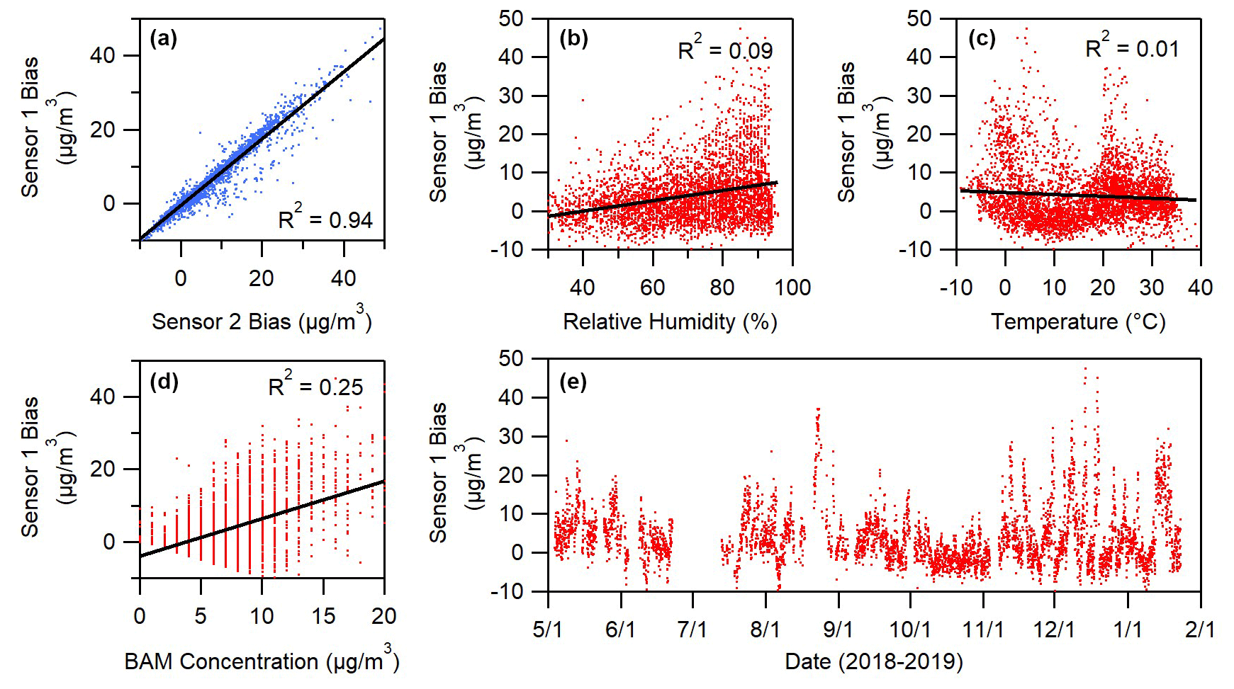
Figure 2 Panel (a) shows the correlation between the bias (C_sensor−C_reference) of two sensor replicas. Panels (b)–(d) show correlation between sensor bias and meteorological factors. Panel (e) shows that bias varies over time but not in a consistent pattern. Measurement gaps in (e) are the result of the BAM not meeting its internal relative humidity specification (35 %).

Figure 1 shows that good agreement was observed between measurements from duplicate sensors. Figure 2a supports this observation, showing close correlation between bias, defined as C_sensor−C_reference, for duplicates of a sensor. Figure 2 (y axes) shows that sensor bias typically ranges from 10 below to 40 µg m⁻³ above the reference measurement. It is noteworthy that sensor measurements correlated so closely from one sensor to another (Fig. 2a) despite such a large range of variation from reference measurements. Comparison between only two sensors is shown in Fig. 2a for simplicity, but similarly strong correlation was observed for other pairs of sensors. Others have observed similar correlation between measurements from duplicates of low-cost sensors (Feenstra et al., 2019; Zamora et al., 2020). Because these measurements came from separate sensors (same brand and model) in separate housing, the large yet correlated bias suggests that an external correctable factor influences how accurately sensor measurements correlate with the reference measurement. However, Fig. 2b–e show that only slight correlation was seen between this bias and easily observable external factors like humidity, temperature, particulate matter concentration, or time. Solar radiation, wind direction, wind speed, and rain were also measured, and similarly little correlation was observed between bias and these factors. Other research has observed improved PM_2.5 predictions when parameters such as temperature and relative humidity are included in analysis (Datta et al., 2020; Di Antonio et al., 2018; Gao et al., 2015; Kumar and Sahu, 2021; Levy Zamora et al., 2019; Zou et al., 2021b). Though some improvement in PM_2.5 predictions is still possible using the same approach here, Fig. 2 suggests that these meteorological parameters are not the primary cause of the similar bias that is observed from one sensor to another.

The lack of correlation suggests that a different external factor, such as particle properties, may influence sensor measurements. Previous research has observed the impact of particle composition on the accuracy of low-cost sensors (Giordano et al., 2021; Kuula et al., 2020; Levy Zamora et al., 2019). Particle size has also been observed to influence measurements (Stavroulas et al., 2020; Zou et al., 2021a). Very small particles go undetected and other particles can be incorrectly sized by the optical detectors used in low-cost particulate matter sensors. Regardless of the cause in varying yet correlated sensor response, data here suggest that low-cost measurements of meteorology will not be sufficient to improve low-cost sensor data. It may be possible to improve sensor data through measurements of particle properties, but the high cost of these measurements would undo the benefit of the low sensor price.

3.2 Performance evaluation

The T640 was available for comparisons for approximately 1 month in April 2019. In contrast to the BAM, which reports data only in 1 h intervals, the T640 was programmed to report a measurement every minute, allowing comparisons to the high-time-resolution data offered by sensors. In addition, the month of April provided useful comparisons as elevated concentrations of particulate matter were observed on 3 different days, likely due to nearby agricultural burning. Under different evaluation conditions, the R² and RMSE of a linear regression were calculated. Impacts on R² and RMSE from different averaging time, reference instrument, and higher concentrations are shown in Fig. 3.

Figure 3 The changes to R² and RMSE from a baseline condition depending on evaluation conditions. Panel (b) shows the baseline of 1 h averaged data with T640 as a reference instrument and without 3 d of high concentrations. Panels (a) and (c) show the impact of less and more data averaging, respectively. Panel (d) shows the impact of switching to the BAM instead of the T640. Panel (e) shows the effect of high concentration by including 3 additional days during which higher concentrations were observed.

1 h averaged data comparisons between a sensor and the T640 are used as a baseline for comparison (Fig. 3b). To highlight differences, the 3 d that included high particulate matter concentrations were not included, except when indicated (Fig. 3e). Figure 3a–c shows that less averaging (higher-time-resolution data) negatively impacted R² and RMSE, while more averaging improved both these metrics. Though higher time resolution is often considered an advantage of low-cost sensors compared to some reference measurements, these data show that time resolution comes at a cost in the ability of sensors to predict concentration. If a specific averaging period becomes the standard for evaluations, such as 1 h averaging (Duvall et al., 2021), then sensor users will need to carefully assess how the quality of data changes if it is necessary to average to a different interval, such as 5 or 1 min intervals.

Figure 3d shows the difference in comparison due to reference instrument. The EPA considers both the BAM and the T640 to be FEM instruments, but both the R² and the RMSE are negatively impacted when evaluating with the BAM instead of the T640. The T640 is an optical particle counter, which dries and then counts individual particles. It differs from the evaluated low-cost sensors, which take a nephelometric measurement of un-dried, bulk particle concentrations. However, the T640 is still an optical measurement and is more similar to the method used by low-cost particulate matter sensors. This comparison shows that the choice of a reference instrument in evaluation of sensors can impact results.

Figure 3e is the only panel in Fig. 3 that includes data from the 3 d in April 2019 on which higher concentrations of particulate matter were observed. Most 1 h measurements were below 50 µg m⁻³ during this month, but within these 3 d, there were 24 observations of 1 h particulate matter concentrations between 50 and 400 µg m⁻³. During this month, about 565 1 h data points were captured, but Fig. 3e shows the influence of just a few measurements at higher concentrations. R² in the baseline chart is 0.80, but with the addition of these points it increases all the way to 0.97. In contrast, RMSE increases from 3.2 to 5.9 µg m⁻³ with the addition of these higher-concentration data, suggesting decreased sensor performance. At high concentrations, small percent differences between sensor and reference measurements translate into larger errors when expressed in micrograms per cubic meter (µg m⁻³).

Figure 3 shows that the circumstances surrounding an evaluation such as averaging time, reference instrument, and the presence of high particulate matter concentrations can be very influential on the performance results for a sensor, even with other factors being held equal. The averaging time and the choice of reference instrument could become smaller issues as standard evaluation procedures are developed, such as those recently proposed by the United States Environmental Protection Agency (Duvall et al., 2021). However, the influence of concentration range on R² and RMSE is a challenge in evaluating sensors, as it suggests that evaluation location and random circumstances such as high concentration events are influential on evaluation results. In addition, R² and RMSE are not particularly suited to interpreting a new measurement from a sensor once an evaluation has been completed. As an alternative to R² and RMSE, a prediction interval can be considered as an evaluation tool for low-cost sensors.

A prediction interval (PI) between sensor and reference data offers a robust yet straightforward interpretation of sensor measurements. A 95 % PI suggests that one can be 95 % confident that any new measurement will be within its bounds; thus, a new sensor reading can be converted to a range of estimates with statistical confidence. The width of this PI is a useful way to show the performance of the sensor. Though a PI is calculated from a linear regression just like R² and RMSE, it requires a few extra details. The most important of these details is that the residuals of the linear fit need to be even across the range of observed values. In the data described here, and likely for other low-cost sensor data, this will require a transformation to the data.

Figure 4 shows the PI for data that were collected at 5 min intervals in April 2019. After fitting a linear regression to these data, it was found that residuals generally increased with increasing concentration, suggesting that bias can be higher as concentrations increase. This is also seen in the Fig. 2d comparison between low-cost sensor bias and BAM measurements. In order to ensure a correct linear fit and PI, these trends in residuals were eliminated by transforming both the sensor and reference data prior to the fit. Through examination it was found that residual trends were best eliminated by raising both the sensor and reference data to the 0.4 power. Future applications of this method to various sensors may find that different powers or transformation methods are needed to eliminate trends that are observed in residuals. Even duplicates of the same sensor may require different transformations if taking measurements in different locations. A detailed analysis of residuals is an important step in all model development. In addition to the transformation, measurements less than 70 µg m⁻³ were randomly sampled to capture an equal number of data points below and above 70 µg m⁻³. This sampling did not change the outcome significantly, but helped ensure that the linear regression and PI were equally weighted to the entire range of observed measurements. Before this sampling only 5 % of the data were above 70 µg m⁻³. The R software suite was used to calculate the linear regression and PI for the transformed data, and these curves were then reverse-transformed (raised to the 0.4⁻¹ power) to create the graph shown in Fig. 4.

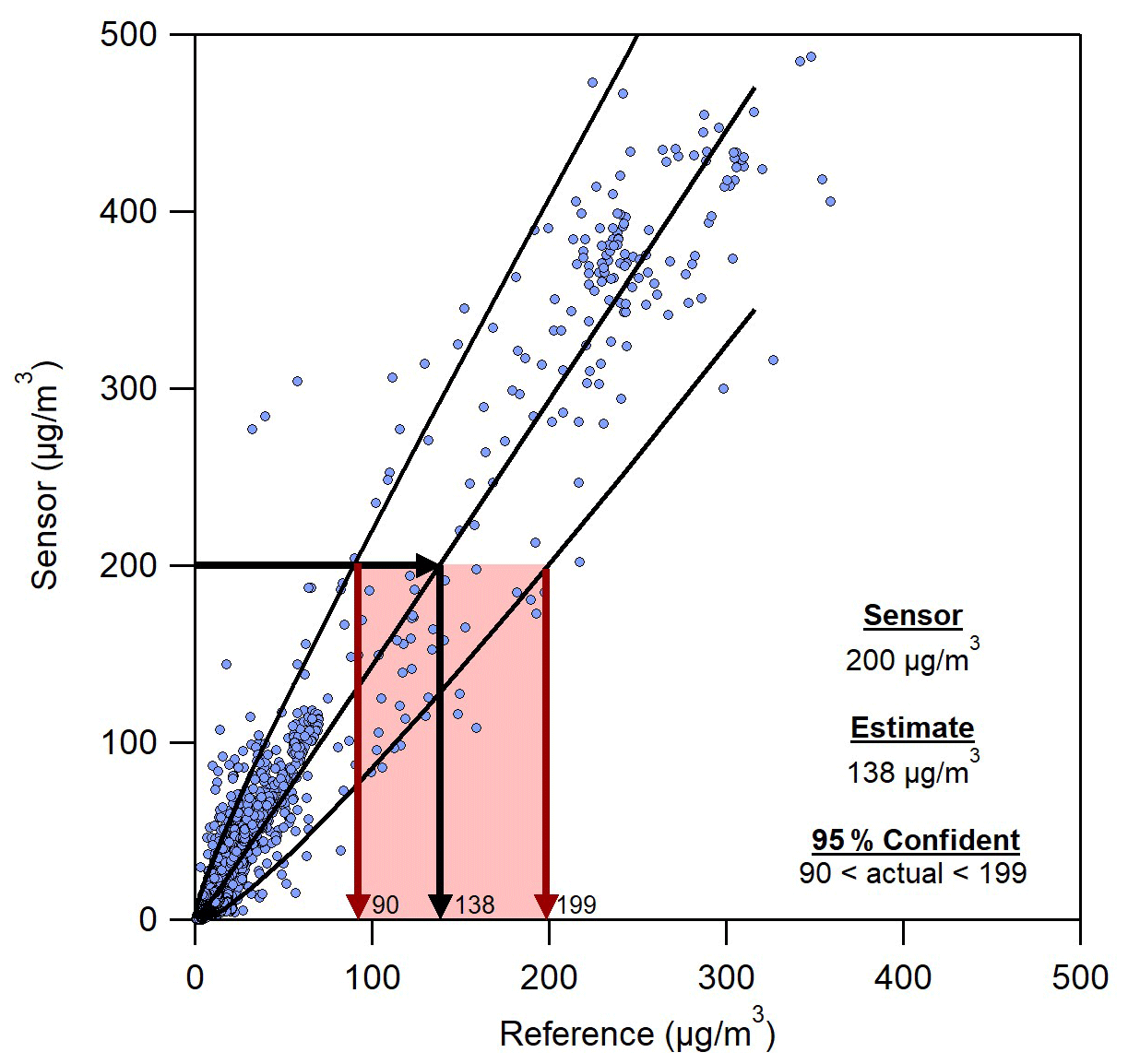
Figure 4 An example of a prediction interval evaluation for 5 min data from a single sensor in April 2019 that includes periods of high concentration. The curved lines are the upper and lower limits of the 95 % prediction interval. A visual interpretation of a new sensor measurement of 200 µg m⁻³ is also shown.

Once data have been analyzed using the method shown in Fig. 4, the interpretation of new sensor data becomes easy. As shown in Fig. 4, a new sensor measurement at 200 µg m⁻³ suggests the most likely actual concentration is 138 µg m⁻³. However, more importantly, it can be said with 95 % confidence that the true concentration is between 90 and 199 µg m⁻³. Replicating this analysis for similar data from another sensor suggests that for a sensor reading of 200 µg m⁻³ the most likely concentration is 148 µg m⁻³, with a 95 % prediction interval between 97 and 213 µg m⁻³. These estimates are close to those from the first sensor, showing again that precision is good for these sensors. Data from multiple replicas of a sensor could also be combined to provide a more general prediction interval that applies broadly to sensors of that type. If sensors are not very precise then the combined data will have higher variance, which will lead to an appropriately broader prediction interval and higher uncertainty in estimates for future sensor measurements. Any nonlinearity in sensor response (Zheng et al., 2018) will also result in a broader prediction interval if it has not been accounted for in the calibration model.

A range can be provided for any new sensor measurement following this method with 95 % confidence. In some cases that uncertainty range may limit the ability to distinguish one concentration from another. For example, in Fig. 4 the estimated ranges for 5 min averaged sensor measurements of 150 and 200 µg m⁻³ will overlap significantly, so it would not be clear whether those measurements capture different concentrations or multiple measurements at the same concentration. However, 5 min averaged sensor measurements of 30 and 200 µg m⁻³ will clearly show a difference between measurements, even with the uncertainty in those measurements. It is notable that the relationship between uncertainty and sensor concentration is nonlinear. This nonlinearity is a detail that would not be captured using RMSE or normalized RMSE to describe uncertainty in measurements.

Figure 5 shows the dependence of average uncertainty on the concentration (sensor estimate) and on the averaging time. For the sake of simplicity Fig. 5 only shows the average difference between the sensor estimate and both the upper and lower PI. In the example in Fig. 4 uncertainty would be calculated as (199–$\mathrm{138}\mathrm{\mu }\mathrm{g}{\mathrm{m}}^{-\mathrm{3}})/\mathrm{2}+(\mathrm{138}$–$\mathrm{90}\mathrm{\mu }\mathrm{g}{\mathrm{m}}^{-\mathrm{3}})/\mathrm{2}$. Generally, sensor uncertainty increases with concentration, though it does so nonlinearly. For 5 min averaged data the uncertainty is ±22 µg m⁻³ when actual concentration is 30 µg m⁻³, but this rises to ±88 µg m⁻³ for measurements of 300 µg m⁻³. When averaging times are lengthened and more data are included in each measurement the uncertainty ranges can change significantly. For example, a measurement of 20 µg m⁻³ has uncertainty of ±17, ±12, and ±4.4 µg m⁻³ for averaging times of 5 min, 1 h, and 1 d.

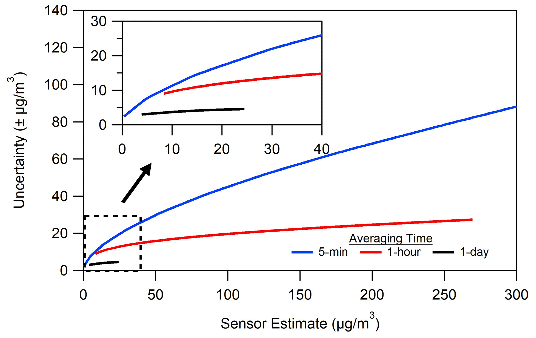
Figure 5 An alternative view of the prediction interval, which shows how this interval varies with concentration and with averaging time.

A PI evaluation such as that shown in Figs. 4 and 5 offers more information about what to expect from future sensor measurements versus R² or RMSE. A future 5 min averaged sensor measurement of 200 µg m⁻³ is more meaningful if it can be quantified with the statement that there is a 95 % probability that the actual concentration is between 90 and 199 µg m⁻³. An evaluation with a PI also allows for better comparison between sensors, as the evaluation results are not influenced by the range of concentrations observed during evaluation. Uncertainty at a specific concentration can be compared from one brand of sensor to another and is not impacted by the range of concentrations observed, in contrast to RMSE or R². In other words, the uncertainty of a sensor at 35 µg m⁻³ does not change depending on whether concentrations of 100 µg m⁻³ were also measured during evaluation, though the overall R² or RMSE of that evaluation can be influenced by the 100 µg m⁻³ measurements, as shown in Fig. 3. An analysis such as that shown in Fig. 5 also allows a user to see how averaging time and concentration change the meaning of a sensor measurement.

Picking a single comparison point allows users to quickly compare measurement uncertainty between different sensor types, as they might currently using R² or RMSE. The break points in the United States Air Quality Index (AQI) could be considered standard comparison points. For example, the United States AQI transitions to “unhealthy for sensitive groups” at 35 µg m⁻³. At this level three sensor replicas showed uncertainty of 14, 16, and 20 µg m⁻³.

3.3 Trends over time

The analysis shown in Figs. 4 and 5 relies on a user collecting enough data to predict the PI bounds that capture 95 % of future data points. Without sufficient data the PI will be incorrect or will only cover measurements over a limited range. This is illustrated in the 1 d averaged uncertainty in Fig. 5, where uncertainty is only calculated for concentrations ranging from approximately 5 to 25 µg m⁻³ due to limited data. The amount of time it will take to collect enough data to build a PI analysis for sensor data will vary from one location to another and is explored for this location in Fig. 6. This figure outlines an approach to determine the amount of time needed to calibrate a sensor using a PI, as described in Sect. 3.2, or any other method.

Figure 6 Linear regression parameters from 1 h measurements over a 2-month period in 2018. Panel (a) shows the range of measurements observed on each day. Panels (b)–(d) show the R², slope, and residual standard error, respectively. In (b)–(d) a rolling collection of 1, 7, or 14 d of data was used to find linear regression parameters.

Figure 6 shows variations to linear fit parameters between 1 h averaged sensor and reference measurements collected during a 2-month period. Figure 6a shows the range of values observed each day during this period. In Fig. 6b–d a linear regression is calculated for 1 h measurements in a rolling timeframe of 1, 7, or 14 d. Figure 6b shows that with just 1 d of 1 h averaged data, R² is sporadic from one day to the next. It is much more consistent over time when 7 d of data are used, but even then there are periods that are inconsistent with the rest of the data. For example, the R² for a 7 d comparison between sensor and reference data centered around 24–26 November is lower than at other times. This inconsistency is eliminated when using 14 d of data.

Just as for R², Fig. 6c shows that a sporadic trend is also observed for slope when fitting a linear regression on just 1 d of data at a time. Notably, the confidence interval on the slope (shown as shaded area) often dips below 0, suggesting a lack of statistical confidence that a trend has been observed. Slope is much more consistent using 7 d of data, though as with R² there is a 7 d period in November (centered around 24–25 November) during which slope is different. Using 14 d of data eliminates the abnormal period in November, but a difference is still observed between the slope in October and November. This suggests that 14 d is an improvement compared to 7 d, but even 14 d may not be enough collocation time for a thorough calibration.

Figure 6d shows residual standard error over time, which can be used as a surrogate for the width of a PI. Calibrations using 1 d of data often have low error, as they include only a narrow range of concentrations. The residual standard error changes over time, even using 7 and 14 d intervals. All variations in residual standard error should be captured for a thorough calibration. It is especially important to capture the maximum in residual standard error to ensure that the prediction interval captures the full range of uncertainty in future measurements.

In short, Fig. 6 shows that even with up to 7 or 14 d of data, variations in linear regression parameters are still observed. Considine et al. (2021) observed that approximately 3 weeks were needed for a simple linear sensor calibration, and 7–8 weeks were required if using a more complicated correction such as machine learning. Duvall et al. (2021) recommended 30 d to develop a calibration. The goal of any calibration for low-cost particulate matter sensors should be to observe all variations in particle size, composition, and concentration. Thorough calibrations may require lengthy periods of collocation to capture all variations in these parameters and in the range of concentrations observed. An analysis of linear fit parameters over time such as in Fig. 6 can be helpful in determining if the full range of situations has been observed and captured by the resulting calibration model.

3.4 Calibration implications

Understanding the behavior of low-cost particulate matter sensors over time is important in planning for the amount of data required to calibrate the sensor. The results presented in this study are useful in analyzing the strengths and weaknesses of different calibration methods. Stanton et al. (2018) outlined four methods that could be used to capture sensor and reference measurements for calibration.

• Routine collocation. Sensors are placed near the reference instrument for a period before deployment. They may be brought back periodically for re-calibration.

• Permanent collocation. One sensor is placed next to a reference instrument with the assumption that any correction needed for that sensor applies to the others in the network.

• Mobile collocation. A reference instrument is placed on a vehicle, and all sensors receive a single-point calibration update when the reference comes within proximity.

• “Golden sensor”. One sensor is calibrated via collocation with a reference instrument and then slowly moved throughout the network to calibrate the other sensors.

The routine collocation method is a useful starting point in any sensor network. A period of side-by-side sensor and reference data captures the slope, intercept, and typical error that is associated with sensor measurements. Figure 6 suggests that this method will have mixed results if calibrating over short time periods but can be reliable given enough time to capture all variations in slope, concentration, and residual standard error. The method does not capture the location bias that may be observed if sensors respond differently to the particles at the sensor location compared to those at the calibration location. Despite these limitations, Fig. 6 suggests that this method can likely improve sensor data if utilized appropriately.

The precision between sensors (see Fig. 2) suggests there is potential for a routine collocation method to greatly improve data, though there may be difficulties in accounting for location bias. The question remains of how much distance can be allowed between the reference sensor and the field-deployed network sensors before this method fails. This allowable distance will depend on how quickly particle properties change between the reference instrument and the network of sensors.

A mobile approach to calibration is attractive in that it can be used to capture variations in sensor responsiveness at different locations with different types of particles compared to those at a fixed reference location. The challenge with this approach will be capturing enough data to thoroughly understand the slope and prediction interval of sensor measurements. Figure 6 shows that even using 24 1 h data points can lead to unusual estimates for the slope between sensor and reference measurements, and a single-measurement spot check between a mobile reference and a sensor would likely be even more sporadic. It is possible that these single-measurement spot checks could slowly improve an existing calibration over time, but whether that improvement happens within a reasonable timeframe is something that would require more exploration.

The “golden sensor” method relies on a calibrated sensor to calibrate other sensors in the network. The challenge with this approach is that the actual concentration is not known once the sensor has left the reference instrument. At this point measurements are just an estimate with a 95 % confidence interval. The level of uncertainty in measurements (see Fig. 4) would make it very challenging to pass a calibration from one sensor to another without greatly increasing uncertainty.

Regardless of the choice of calibration method, it is important to consider variations in sensor data when conducting a calibration and when interpreting future sensor results. As Fig. 6 shows, calibrations may take weeks or longer in order to capture all variations in the external factors that influence sensor response. If these variations are not captured correctly, then the resulting calibration may miss important changes to sensor response that occur due to changing environmental variables. Reliance on a calibration that does not account for all variance in measurements may make sensor data less reliable. A calibration that also provides a PI ensures that future results can be interpreted with statistical rigor.

4 Conclusions

Low-cost sensors have potential to provide a better understanding of temporal and spatial trends of pollutants like particulate matter. Evaluations of low-cost particulate matter sensors alongside reference instruments in Bartlesville, Oklahoma, have been used to identify methods that ensure more consistent evaluation and interpretation of sensor data.

Bias in sensor measurements varied over time but was very closely correlated from one sensor to the next (see Fig. 2). Because bias is so closely correlated, sensors can be deployed in pairs as a simple way to identify erroneous measurements (see Fig. 1). Finding ways to efficiently and effectively determine sensor performance is critical as sensors become more widely adopted. Two of the most popular evaluation metrics, R² and RMSE, can be influenced by averaging time, choice of reference instrument, and the range of concentrations observed (see Fig. 3). This study shows how a prediction interval can be used as a more statistically thorough evaluation tool. A PI offers a more robust method of sensor evaluation and a statistical confidence interval for interpretation of future sensor measurements (see Fig. 4). When properly applied, this method can show how uncertainty in sensor measurements varies as a nonlinear function of observed concentrations and also varies with the averaging time for measurements (see Fig. 5). A standard ambient PM_2.5 concentration could be chosen for simple comparisons of uncertainty between sensors. For example, uncertainty measurements from multiple sensors at 35 µg m⁻³ would allow convenient comparisons. Standardization of comparison concentration, reference instruments, and averaging times would allow more thorough decisions about which sensor is best suited to a proposed task. Building an effective prediction interval, linear regression, or any other calibration model depends on capturing the necessary data (see Fig. 6), and careful thought is required in planning the method and length of time for a calibration. The work presented here shows how adjustments to low-cost particulate matter sensor evaluations can greatly improve the interpretation of future data.