the Creative Commons Attribution 4.0 License.
the Creative Commons Attribution 4.0 License.
 | 03 Feb 2021
Generalized canonical transform method for radio occultation sounding with improved retrieval in the presence of horizontal gradients
Michael Gorbunov
Gottfried Kirchengast
Kent B. Lauritsen
By now, a series of advanced wave optical approaches to the processing of radio occultation (RO) observations are widely used. In particular, the canonical transform (CT) method and its further developments need to be mentioned. The latter include the full spectrum inversion (FSI) method, the geometric optical phase matching (PM) method, and the general approach based on the Fourier integral operators (FIOs), also referred to as the CT type 2 (CT2) method. The general idea of these methods is the application of a canonical transform that changes the coordinates in the phase space from time and Doppler frequency to impact parameter and bending angle. For the spherically symmetric atmosphere, the impact parameter, being invariant for each ray, is a unique coordinate of the ray manifold. Therefore, the derivative of the phase of the wave field in the transformed space is directly linked to the bending angle as a single-valued function of the impact parameter. However, in the presence of horizontal gradients, this approach may not work. Here we introduce a further generalization of the CT methods in order to reduce the errors due to horizontal gradients. We describe, in particular, the modified CT2 method, denoted CT2A, which complements the former with one more affine transform: a new coordinate that is a linear combination of the impact parameter and bending angle. The linear combination coefficient is a tunable parameter. We derive the explicit formulas for the CT2A and develop the updated numerical algorithm. For testing the method, we performed statistical analyses based on RO retrievals from data acquired by the Constellation Observing System for Meteorology, Ionosphere, and Climate (COSMIC) and collocated analysis profiles of the European Centre for Medium-Range Weather Forecasts (ECMWF). We demonstrate that it is possible to find a reasonably optimal value of the new tunable CT2A parameter that minimizes the root mean square difference between the RO retrieved and the ECMWF refractivity in the lower troposphere and allows the practical realization of the improved capability to cope with horizontal gradients and serve as the basis of a new quality control procedure.
- Article
(3797 KB) - Full-text XML
- BibTeX
- EndNote


The first step in the development of the wave optical (WO) approach to the processing of radio occultation (RO) observations was made by Melbourne et al. (1994) who used the thin screen approximation for the atmosphere combined with the back propagation (BP) technique. This approach was further developed under the name of Fresnel inversion by Mortensen and Høeg (1998). Although the accuracy of this approximation in the lower troposphere was insufficient for practical application, its basic idea was correct. It consisted in the reduction of the influence of the diffraction by using the BP, which made the inversion results independent from the observation distance and canceled the resolution restriction due to the Fresnel zone size.
Later works (Gorbunov et al., 1996a; Karayel and Hinson, 1997; Gorbunov and Gurvich, 1998a, b) developed a different understanding of the BP technique. The BP wave field evaluated in some plane was not considered as the actual wave field but as a representation of the original field observed at low Earth orbit (LEO); in this representation, the effects of diffraction and multipath propagation were significantly reduced. This, in a straightforward way, allowed the evaluation of the geometric optical (GO) bending angle profile, which was inverted in the framework of the standard GO scheme (Ware et al., 1996; Kursinski et al., 1997).
The further development of the WO approach based on the representation view relied upon the concept of the canonical transform (CT) originating from classical mechanics (Arnold, 1978; Goldstein et al., 2014), generalized for quantum mechanics by Fock (1978) and mathematically substantiated by Egorov (1985) and Egorov and Shubin (1993). Later on, this concept obtained an extensive mathematical development (Treves, 1982a, b; Hörmander, 1985a, b). The correspondence between quantum and classical mechanics is the same as the link between wave optics and geometrical optics.
In both cases, there is a strict mathematical representation (quantum mechanics or wave optics) and its asymptotic solution (classical mechanics or geometrical optics). While the evolution of de Broglie waves of probability or electromagnetic waves is described by the Hamilton operator, the evolution of rays or classical trajectories of particles is described by the Hamilton system. The Hamilton operator is obtained from the Hamilton function by the substitution of the momentum operator instead of classical momentum. Accordingly, for the classical problem, the phase space is introduced, the dimension of which equals double the geometric dimension because to each geometrical coordinate, we can conjugate the corresponding momentum. For the wave problems, momentum is understood as the ray direction vector.
The canonical transforms arise when we consider the class of the transforms of the phase space that conserve the canonical form of the Hamilton dynamical system. It was first demonstrated by Fock (1978) that these transforms have a very simple implementation in quantum mechanics: they correspond to linear transforms of the wave function. The kernel of this transform is derived in classical terms, but still it describes a short-wave asymptotic solution of the wave problem. This idea was later mathematically developed first by Egorov (1985) and Egorov and Shubin (1993) and then by Treves (1982a, b) and Hörmander (1985a, b).
The application of the CT approach for the RO observation processing was pioneered by Gorbunov (2002), who combined it with the BP. The idea of the CT without BP was first developed by Jensen et al. (2003, 2004), and later the general view of these results in the framework of the CT approach was developed by Gorbunov and Lauritsen (2004a, b). Finally, it was recognized that the different methods – CT (Gorbunov, 2002), full spectrum inversion (FSI) (Jensen et al., 2003), phase matching (PM) (Jensen et al., 2004), and CT of the second type (CT2) (Gorbunov and Lauritsen, 2004a) – were, in fact, different approximations of the same solution, for which Fourier integral operators (FIOs) provided the general transform approach (Gorbunov and Lauritsen, 2004a).
The idea of the CT approach is as follows. Given the observations or RO complex signal u(t) as a function of time t, which can be represented through its amplitude A(t) and phase ϕ(t), u(t)=A(t)exp (iϕ(t)). It is convenient to use eikonal or phase path , where is the wavenumber, and λ is the wavelength. Thus, u(t)=A(t)exp (ikΨ(t)), and k is the large parameter. The signal is composed of multiple sub-signals ui(t)=Ai(t)exp (ikΨi(t)) corresponding to interfering rays. For each sub-signal, it is possible to introduce the instantaneous frequency . However, the instantaneous frequency cannot be introduced for their composition.
The multipath propagation problem consists in the decomposition of the signal equal to the sum or different sub-signals to retrieve the ray structure of the observed field. The solution of this problem discussed in the aforementioned papers consisted in the transform of the observed wave field u(t) into a different representation. The new coordinates in the transformed space were the ray impact parameter p and bending angle ϵ. The transform is canonical (Gorbunov and Lauritsen, 2004a), which allows for writing the corresponding linear transform , where the subscript 2 indicates that it is a CT of the second type (Arnold, 1978; Goldstein et al., 2014) that maps the original field u(t) to a field in the impact parameter representation . The idea of the choice of the ray impact parameter as the new coordinate is based on the fact that in a spherically symmetric medium, the ray impact parameter is the ray invariant, which is known as Bouguer's law. The locally spherically symmetric medium is the basic approximation used in the inversion of RO data. For the real atmosphere with horizontal gradients, the dynamic equation for p was derived by Gorbunov and Kornblueh (2001), who demonstrated that the derivative of p with respect to the ray arc length is equal to the horizontal component of the refractivity gradient in the occultation plane. Strong horizontal gradients may result in the situation when dependence ϵ(p) becomes multivalued (Healy, 2001; Gorbunov and Lauritsen, 2009), which was referred to as the impact parameter multipath (Zou et al., 2019).
The idea explored in the present manuscript consists in the further development of the CT approach by using a generalized transform with the coordinate . Unlike the standard CT approach, for which the form of the new coordinates in the phase is known in advance, this transform has the tunable parameter β that can take into account the statistical impact parameter multipath effect.
The paper is organized as follows. In Sect. 2, we discuss the canonical transform in wave optics and quantum mechanics in general terms, including a brief review of FIOs. Based on this context, we discuss in Sect. 3 the application of the CT method for RO and introduce the particular phase space and the specific choice of coordinates, as well as the new generalization, adding an affine transform with a tunable parameter for improving the coping capability with horizontal gradients. In Sect. 4, we discuss the practical modifications needed to readily advance existing numerical implementations of the CT algorithm and present results of our performance evaluation from processing actual observed Constellation Observing System for Meteorology, Ionosphere, and Climate (COSMIC) RO data, including how to find an optimal value of the tunable parameter to minimize the retrieval errors in the lower troposphere. Section 5 finally provides the summary and main conclusions of the paper.
The canonical transforms (CTs) in classical mechanics are a class of transforms of the coordinates and momenta conserving the Hamiltonian form of the dynamical equation (Arnold, 1978; Goldstein et al., 2014). Fock (1978) introduced the CT into quantum mechanics. Note that the first Russian edition of the monograph by Fock appeared as early as 1929. Because the relation between classical and quantum mechanics, on one side, and the relation between geometrical and wave optics, on the other side, are the same, we can immediately apply the approach introduced by Fock (1978).
We assume that the wave field can be represented in the standard form:
where t is the observation time, Ψ(t) is the eikonal, is the wavenumber, λ is the wavelength, and A(t) is the amplitude. The time t can be associated with a specific spatial location of the observation, as is the case in RO, but u(t) can also be looked at as a generic signal.
The amplitude A(t) and the derivative of Ψ(t) are assumed to be slowly changing within an oscillation period. In this case, the wave field is termed quasi-monochromatic with an instant amplitude A(t) and frequency . Otherwise, more generally, the field should be equal to a super-position of quasi-monochromatic components:
where the upper index j enumerates the components, A(j)(t) are their amplitudes, and Ψ(j)(t) are their eikonals. Each component has its own instant amplitude and frequency.
When discussing the CTs, it is necessary to bear in mind that most of the relations have an asymptotic nature, in which k is the large parameter (or λ is the small parameter). The reason is as follows. Given measurements of wave field, each monochromatic component can be interpreted in terms of wave fronts and rays defined in terms of instant tones of the signal. At the observation point at time moment t, each component has a single ray, and its direction is linked to the normalized frequency through the geometry of the observation trajectory.
Therefore, for a specific class of signals, including quasi-monochromatic ones and their superpositions, it is possible to introduce a phase space (t,σ). Although the original signal is 1-D, this space is 2-D, and the structure of the signal can be described in terms of the function σ(t) which can be both single valued for quasi-monochromatic signals or multivalued for their superpositions.
Consider RO observations. The original signal corresponds to a range of rays starting at the transmitter and the phase space σ(t) is a very smooth continuous line. As the signal propagates through the atmosphere, its structure gets more and more complicated. Still, in the phase space, its topological structure remains the same; it is always a single continuous line, although it may not be single-valued with respect to time t, which corresponds to multipath propagation (Gorbunov, 2002; Gorbunov and Lauritsen, 2004a). Such a line representing the signal structure is referred to as the ray manifold (Mishchenko et al., 1990).
The outstanding and still simple idea of Fock (1978) was that the classical CTs correspond to linear integral transforms of the wave field with oscillating kernels. This class of transform was later named Fourier integral operators (FIOs) (Egorov, 1985; Egorov and Shubin, 1993; Treves, 1982a, b; Hörmander, 1985a, b). The general form of such an operator first discussed by Fock (1978) has the following form:
where p is a new coordinate in the mapped space. We use notation Φ2 and, accordingly, a2 and S2 because this type of operator was referred to as the FIO of the second type (Gorbunov and Lauritsen, 2004a), while the FIO of the first type is the composition of a Fourier transform and a second type FIO (Egorov, 1985; Egorov and Shubin, 1993). This type of operator is linked to the corresponding type of the CT generating function (Arnold, 1978; Goldstein et al., 2014). Note that historically FIOs of the second type appeared first, but in mathematical works, it was FIOs of the first type that were discussed first.
Considering now u(t) as a quasi-monochromatic signal, we can derive the asymptotic form of transform (Eq. 3) using the stationary phase principle:
The stationary phase point ts(p) of this integral satisfies the equation
Accordingly, the transformed field, under the assumption that Eq. (5) has a single solution ts(p), is also quasi-monochromatic and can be written as follows:
Its instantaneous frequency equals the following:
by virtue of Eq. (5). Recalling that , which is the original momentum, we have the following relation between the canonical coordinates (t,σ) and (p,ξ) in the original and mapped spaces:
which can be expressed in terms of the differential dS2:
and, vice versa, the requirement that the right-hand part in Eq. (9) should be equal to a full differential dS2 of a function S2(p,t) is a necessary and sufficient condition for the transform to be canonical (Arnold, 1978; Goldstein et al., 2014). The function S2(p,t) is then termed the generating function of the canonical transform.
In terms of FIO, S2(p,t) is referred to as its phase function, and a2(p,t) is its amplitude function. The phase function, which specifies the canonical transform, is of primary importance, while the amplitude function is derived using energy conservation (Gorbunov and Lauritsen, 2004a). We see, therefore, that by using classical or geometric optical concepts, it is possible to write down the asymptotic form of the quantum or wave optical operator, implementing the transformation of the original signal into a different representation. If the structure of the original signal is represented as a ray manifold in the phase plane, such a transform is applied to the coordinates in this space. In particular, it may be possible to find such a coordinate system in which the ray manifold geometry will be exceptionally simple.
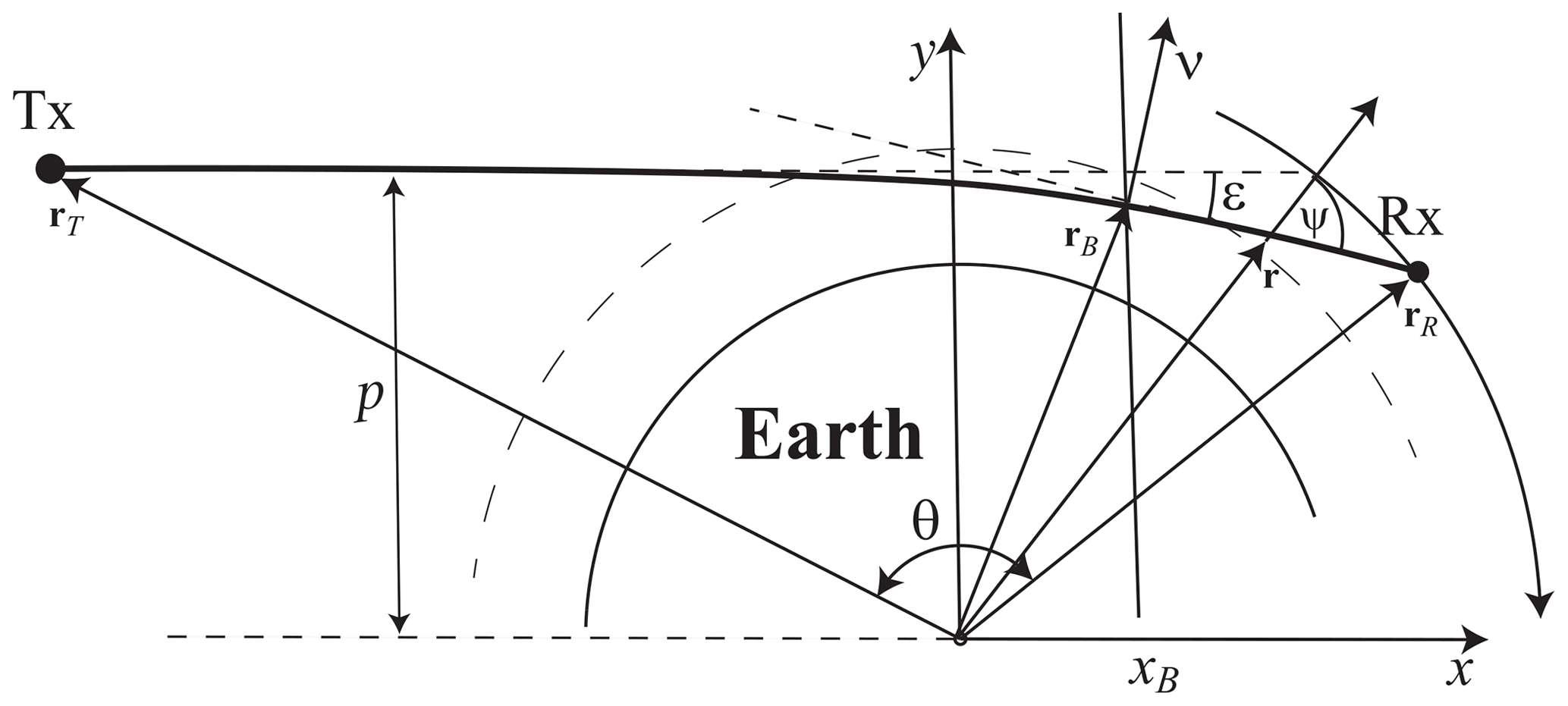
Figure 1Radio occultation observation geometry with relevant geometrical variables indicated (for description see Sect. 3.1)
Here we discuss the application of the CT technique for the analysis of RO observations (Fig. 1) by first reviewing the different existing variants (Sect. 3.1) and then introducing the new generalized CT method (Sect. 3.2) and an application-relevant formulation for readily updating existing algorithms (Sect. 3.3).
3.1 Canonical transform method in different existing variants
The RO observation geometry is schematically represented in Fig. 1. The wave emitted by a transmitter Tx is received by a receiver Rx in low Earth orbit. The transmitter is borne by a satellite belonging to one of the modern Global Navigation Satellites Systems (GNSS), including GPS, GLONASS, Galileo, etc. Due to the movement of the transmitter and receiver, the ray descends or ascends in the atmosphere, which allows for the derivation of the atmospheric profiles from the bending angles ϵ(p) (Ware et al., 1996; Kursinski et al., 1997). The CT technique is used for the retrieval of the bending angle profile from the wave field measurements.
The first approach of processing RO data, belonging to the class of CT, was back propagation (BP) (Gorbunov et al., 1996a; Karayel and Hinson, 1997; Gorbunov and Gurvich, 1998a, b). In this technique, the field was linearly transformed to be recalculated to the BP plane locate at coordinate xB:
where 2-D vector rB(y) equals (xB,y), and ϕ(a,b) is the angle between vectors a and b. This transform is preceded by the stationarization of the transmitting satellite and projection of the satellite movement to the vertical plane. It is important that the BP field is not the real field in the BP plane because the BP procedure assumes vacuum propagation. This procedure results in some representation of the original wave field with reduced diffraction effects due to the reduction of the propagation distance. The new coordinate y is more favorable for finding a unique projection of the ray manifold that disentangles the multipath propagation. Still, this coordinate is not the best choice.
A much better coordinate for the new representation should be the impact parameter p because in a spherically symmetric medium, it is an invariant for each ray due to Bouguer's law, and thus it is unique for each ray. A dynamic equation for the variation of p along the ray as a function of the horizontal gradient of refractivity was obtained by Gorbunov and Kornblueh (2001). The idea of complementing the BP technique with one more transform that maps the field to the impact parameter representation was pioneered by Gorbunov (2002). It was the first application of the FIO of the first type, which has the form
where the only difference from the second type operator is that it acts upon the Fourier-transformed field . It can be looked at as the composition of the Fourier transform, which itself is a second type FIO and another second type FIO. Because the Fourier transform is a simple rotation of the phase space by π∕2: , the equation for the phase function of the first type takes the following form (Arnold, 1978; Goldstein et al., 2014):
Gorbunov (2002) applied this operator to the back-propagated field. To this end, using the normal vector to the straight ray, we express the impact parameter:
Now it is necessary to find the canonical transform whose characteristic property in the 2-D case is the conservation of the volume element, as follows from Eq. (12):
It is enough to consider solutions ξ=ξ(η). Then, from Eq. (14), we readily derive
This results in the solution for the phase and amplitude functions:
This defines the FIO, which is applied to the backpropagated wave field uB(y) and produces the mapped field
The derivative ξ(p) of its eikonal is algebraically linked to the bending angle:
where is the transmitter position in the occultation plane. Because the cross term in S2, which depends both on p and η, is linear with respect to p, the integration over new coordinate ξ=arcsin η turns it to pξ, and, therefore, the operator is reduced to the Fourier transform in combination with a nonlinear change in coordinates. This indicates that this operator allows for a fast implementation. A similar idea will be applied below.
The complicated nature of the BP+CT algorithm stimulated further studies (Gorbunov and Lauritsen, 2002, 2004b) where the idea was expressed of applying the FIO directly to the observed wave field u(t), without intermediate and numerically expensive steps like BP. Full spectrum inversion (FSI), developed by Jensen et al. (2003), was the first solution of this type, although with some restrictive assumptions. However, the general solution was just 1 year away; the phase matching (PM) method was developed by Jensen et al. (2004) and then put into the context of the CT approach by Gorbunov and Lauritsen (2004a), who introduced an approach based on the linearized canonical transform that reduced the FIO to the composition of nonlinear coordinate changes and the Fourier transform. This algorithm was termed the second type CT or CT2. An important advantage of the PM and CT2 methods consists in the fact that they operate with the real transmitter and receiver orbits without the stationarization.
In order to arrive at the phase function of the FIO of the second type, consider the expression for the derivative of the phase of the observed wave field:
Using Eq. (8), we derive the phase function:
where θ, rT, and rR are functions of time t. We do not reproduce here the derivation of the amplitude function a2(p,t), which uses simple geometrical considerations (Gorbunov and Lauritsen, 2004a). This phase function, although providing the accurate solution, has a disadvantage: its cross term depending on both p and t, generally speaking, cannot be decomposed as g1(p)g2(t), and the FIO cannot be reduced to a Fourier transform in compositions with nonlinear coordinate changes. This is only possible in some particular cases, e.g., for circular orbits, when the phase function equals pθ, and using θ as a new coordinate instead of time reduces the operator to the Fourier transform. This method was referred to as FSI.
To find an approximate solution that significantly reduces the computational costs at the expense of an insignificant reduction of accuracy, the representation of the approximate impact parameter was introduced. The impact parameter p is a function of t,σ: . We introduce its approximation :
where σ0(t) is a smooth model of normalized Doppler frequency, , and . We now parameterize the trajectory with the coordinate Υ=Υ(t). For brevity, we use the notation u(Υ) instead of u(t(Υ)). For the coordinate Υ and the corresponding momentum η, we use the following definitions:
Finally, we arrive at the following linear canonical transform :
The generating function of this canonical transform is easily computed from the differential equation:
For the new coordinate Υ, we have the following relation:
For circular orbits, this approximation, once again, reduces to FSI. To evaluate the bending angle, we use the fact that the momentum of the field in the mapped space equals −Υ. We also evaluate the accurate impact parameter p as follows. Given the dependence , it is possible to find the corresponding time . Using Eq. (21), we infer
Finally, for each impact parameter p, we determine the coordinate and, therefore, the corresponding moment of time t=t(Υ(p)) when this ray was observed; the bending angle is then evaluated from the geometrical relation:
This method, termed CT2, indicates both a high accuracy and numerical performance. This discourse leads us to the conclusion that there is a family of closely related WO methods that are based on the same principle. The observed wave field is subjected to a linear integral operator with an oscillating kernel that transforms the field into a different representation. The representation is chosen in such a way that the projection of the ray manifold to the new coordinate axis is unique. The operation is also referred to as the unfolding of multipath. Finally, such methods as CT, FSI, PM, and CT2 involve the evaluation of the same integral transform under different assumptions and approximations. The difference in the results of the application of these WO methods is less significant than the difference coming from other parts of RO data processing systems, including cut-off, filtering, and quality control (QC) procedures (Gorbunov et al., 2004, 2011).
3.2 Generalized canonical transform method
All the modifications of the CT approach discussed above relied upon impact parameter p as the unique coordinate of the ray manifold. However, the impact parameter is, generally speaking, not invariant for each ray, and its perturbations due to horizontal gradients may result in breaking the above condition. To see this, consider the ray equations in the Hamilton form. They are derived from the Hamilton function
where p is the momentum, and n(r) is the refractivity field. The Hamilton system has the following form:
where p is the classical momentum. Because , we arrive at the following differential relation between the parameter τ of this system, the ray arc length s, and the eikonal
Equation (29) has a form that is specific for the Cartesian coordinates. Consider an arbitrary coordinate system with the metric tensor gij: ds2=dxigijdxj, where xi are the components of vector r, and we follow the Einstein tensor notation implying the summation over each pair of upper and lower indexes of the same name. If we define the momentum by the relation , the form pdr is invariant, the transform to the new coordinates (pi, xi) is canonical, and the canonical form of the Hamilton system also remains invariant (Arnold, 1978), provided that the Hamilton function is defined as follows:
where gij is the matrix inverse to gij. This results in the following form of the ray equations:
The 2-D approximation (Zou et al., 2002) allows us to treat rays as plane curves. Consider polar coordinates (r,θ) with the metric tensor:
Then we have the following equations:
where ψ is the angle between vectors and r. The angular component of the momentum pθ coincides with the ray impact parameter p, which is invariant in a spherically layered medium but is perturbed by the horizontal gradients (Gorbunov et al., 1996b; Gorbunov and Kornblueh, 2001; Healy, 2001; Gorbunov and Lauritsen, 2009).

Figure 2Impact parameter multipath, old coordinate (impact parameter) lines, and modified coordinate lines.
The variations in the ray impact parameter, which is no longer an invariant coordinate in the ray space, seem to undermine the elegant idea of the CT approach. Still, the CT method can be applied using the same formulas, but the coordinate p will now acquire a different meaning: it will be understood as the “effective impact parameter”, i.e., the impact parameter which would result in the observed Doppler frequency shift if the atmosphere were spherically layered (Gorbunov et al., 2019; Gorbunov and Lauritsen, 2009). Accordingly, the evaluated bending angle will also be the “effective” bending angle. The reason is that for the evaluation of the real bending angle, understood as the angle between the ray directions at the transmitter and receiver, two corresponding values of the impact parameter are required, which cannot be derived from the single variable, the Doppler frequency. This, by itself, is not a significant problem because the assimilation of bending angle profiles can be based on the effective values (Gorbunov et al., 2019) provided that the observation operator correctly implements their evaluation.
More importantly, horizontal gradients may result in multivalued ray manifold projections when using the effective impact parameter p as the coordinate in the mapped space. This situation is termed “impact parameter multipath” (Zou et al., 2019). Theoretically, for any ray manifold perturbation, there always exists an unfolding coordinate transform. This follows from the fact that topologically the ray manifold is always a continuous line without self-crossing. However, this coordinate transform depends on the a priori unknown horizontal gradients of refractivity.
A typical multivalued bending angle profile (Gorbunov and Lauritsen, 2009; Zou et al., 2019) is shown in Fig. 2. From numerical simulations, it can be inferred that there is a kind of asymmetry; the impact parameter multipath manifests itself mostly in ascending spikes but hardly in descending spikes. Accordingly, in order to better unfold the multipath, it must be possible to use another coordinate in such a way that the modified coordinate lines are sloped. Therefore, we modify the transform Eq. (23) in order to use another coordinate,
where β is a tunable parameter and has dimensions of length/angle (km/rad). Although the optimal value of this parameter should be different for individual events, the aforementioned asymmetry results in the conclusion that the preferred value of β is expected to be negative. Therefore, it may be possible to find its optimal value that, in the statistical sense, will minimize errors due to the impact parameter multipath.
The modified canonical transform Eq. (23) is written as follows:
Using the modified function f′(Υ) instead of the original one, we will obtain the expression for the modified FIO . The advantage of this approach is that it can be implemented by a very simple modification of the existing CT2 algorithm. Using the numerical implementation of the modified CT will allow us to study its influence upon the RO inversion statistics in the lower troposphere.
We denote the generalized FIO . Now we can consider the wave field in the impact parameter representation, . The standard CT algorithm corresponds to the evaluation of with β=0.
It is possible to arrive at a quantitative estimate of β based on Gorbunov and Kornblueh (2001), Gorbunov and Lauritsen (2009), and Zou et al. (2019). We expect that , where δp is the typical variation in impact parameter due to the horizontal gradients, and δϵ is the corresponding bending angle variation. Assuming that δp≈0.1 km, and δϵ≈0.01 rad, we arrive at a first quantitative estimate of km/rad.
3.3 Affine transform for updating existing CT algorithms
Modification of existing numerical algorithms may not be so straightforward as it follows from the above mathematical considerations. In order to avoid this, it is possible to complement an existing implementation of any WO-based numerical algorithm by an additional affine transform.
We will now derive the transform between and . We can write the following transform between these representations:
where ξ0 is the reference point. This is an affine transform in the plane. This suggests the abbreviation CT2A for the new generalized form, which stands for the CT2 complemented by the affine transform.
The generating function of transform (36) is defined by
which is equivalent to the following system:
From this, we can conclude that
This phase function defines the FIO of the first type:
Finally, we can write the operator relation
which can be used for the modification of the existing version of operator .
The above derivation allows for one more generalization. We can consider β=β(ξ). In this case, the phase function is derived in a straightforward way:
Using results in a simple analytical expression for S(β) with a set of tuning parameters βj. In this work, we, however, use a constant β.
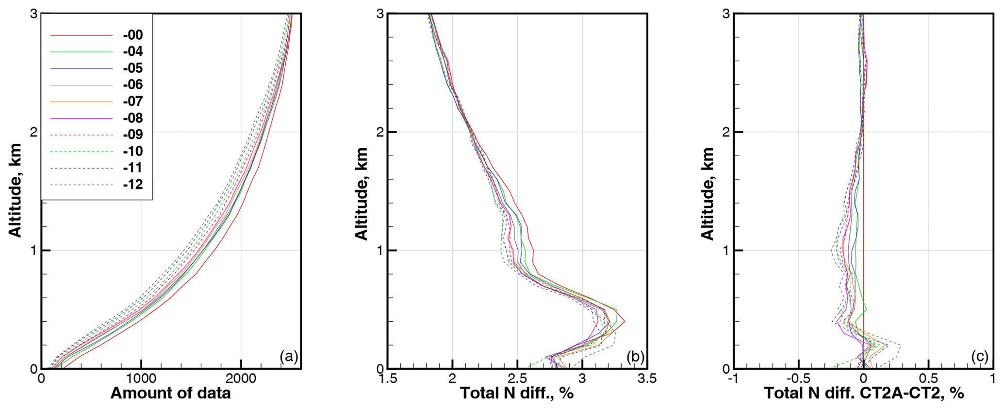
Figure 3Statistics for latitude band 0–10∘. (a) Amount of data. (b) RMS relative difference in refractivity COSMIC–ECMWF ΔNCE. (c) RMS relative difference in refractivity CT2A–CT2. All are functions of the parameter β.

Figure 4Statistics for latitude band 10–20∘. (a) Amount of data. (b) RMS relative difference in refractivity COSMIC–ECMWF ΔNCE. (c) RMS relative difference in refractivity CT2A–CT2. All are functions of the parameter β.
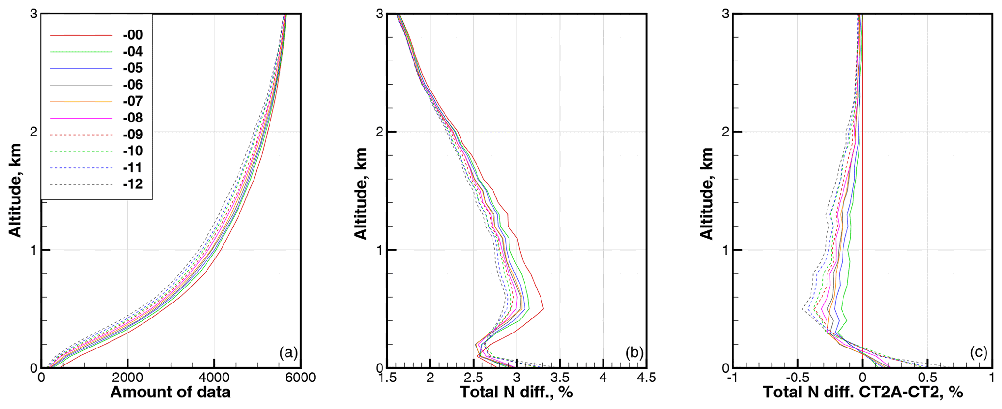
Figure 5Statistics for latitude band 20–30∘. (a) Amount of data. (b) RMS relative difference in refractivity COSMIC–ECMWF ΔNCE. (c) RMS relative difference in refractivity CT2A–CT2. All are functions of the parameter β.
Our implementation of the CT2A algorithm was based on the existing program code with the addition of the parameter β and using the modified function f′(Υ) as defined by Eq. (35). Practically, this only required the modification of a few lines in the program code that implements the CT2 method, as well as the implementation of one more command line parameter.
In our numerical validation, we retrieved COSMIC refractivity profiles NC using COSMIC data from the year 2008 on the 1st and 15th of every month, leading to a total of 24 d and altogether around 60 000 RO events. We used collocated ECMWF refractivity profiles NE, i.e., interpolated to the corresponding COSMIC RO event location, as the reference. To this end, we employed ECMWF analyses at 1∘ latitudinal and longitudinal resolution with 91 vertical levels covering the altitude range up to about 80 km. The refractivity was evaluated from pressure, temperature, and humidity fields. The tangent point drift was taken into account. We used the root mean square (RMS) relative difference in COSMIC from ECMWF ΔNCE, defined as , which includes both systematic and random deviations.
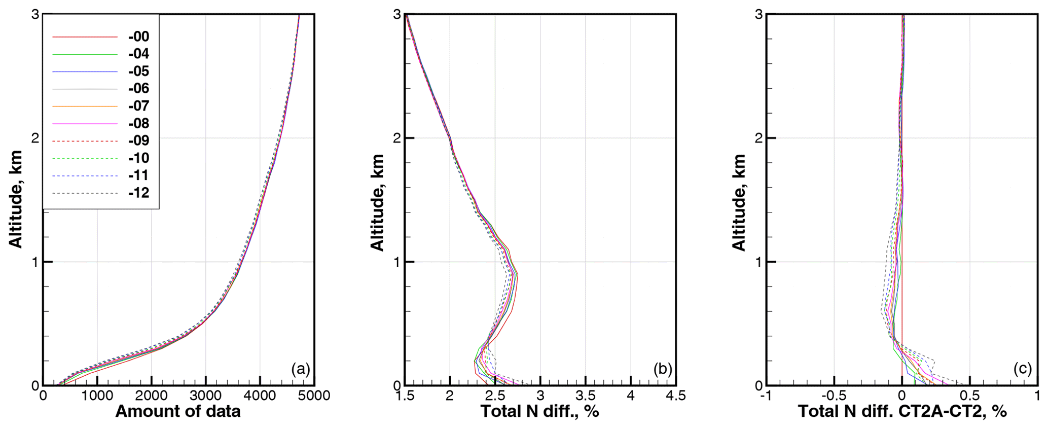
Figure 6Statistics for latitude band 30–40∘. (a) Amount of data. (b) RMS relative difference in refractivity COSMIC–ECMWF ΔNCE. (c) RMS relative difference in refractivity CT2A–CT2. All are functions of the parameter β.
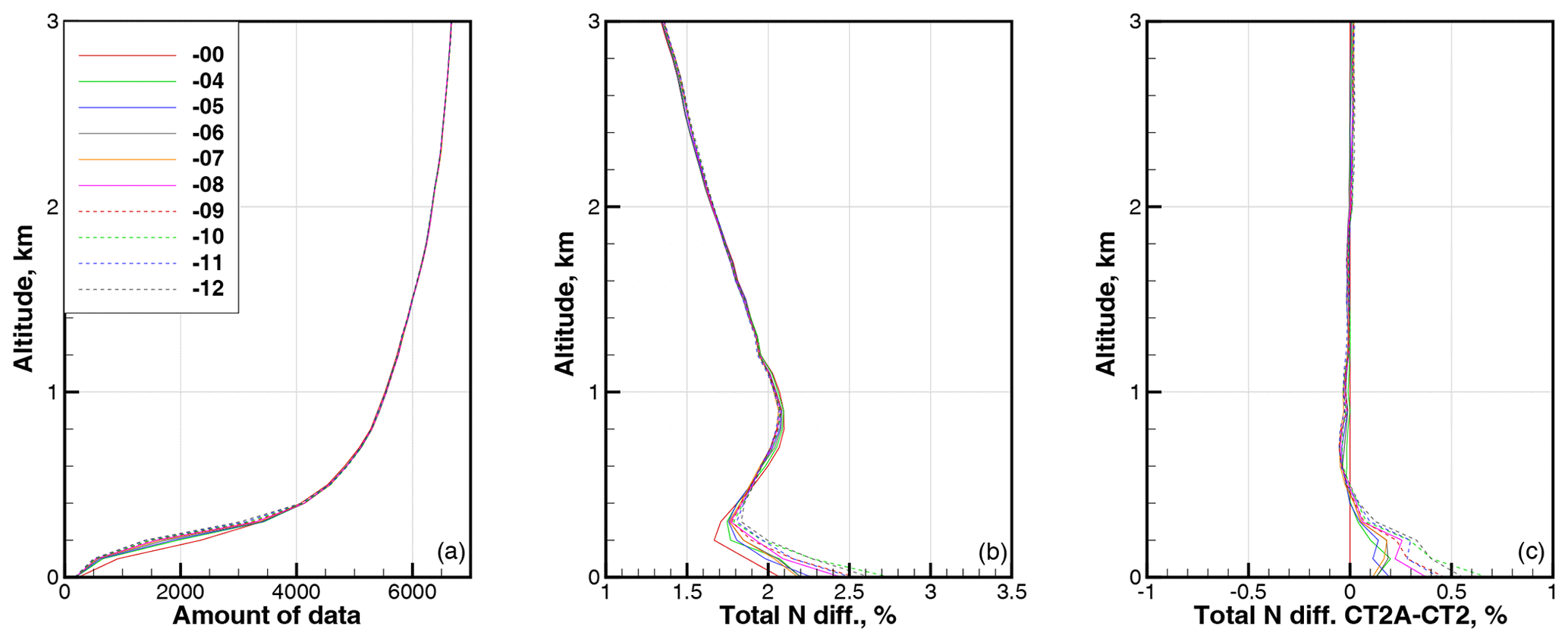
Figure 7Statistics for latitude band 40–50∘. (a) Amount of data. (b) RMS relative difference in refractivity COSMIC–ECMWF ΔNCE. (c) RMS relative difference in refractivity CT2A–CT2. All are functions of the parameter β.
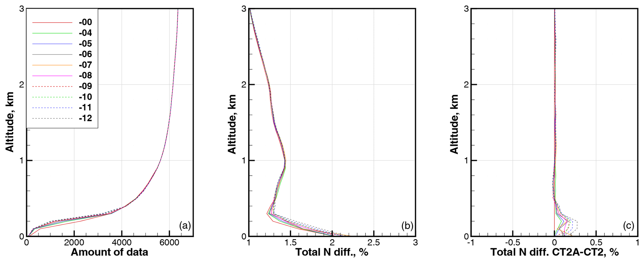
Figure 8Statistics for latitude band 50–60∘. (a) Amount of data. (b) RMS relative difference in refractivity COSMIC–ECMWF ΔNCE. (c) RMS relative difference in refractivity CT2A–CT2. All are functions of the parameter β.
Figures 3 through 11 show the statistical values of ΔNCE as a function of latitude and parameter β. We averaged over 10∘ wide latitude bands including both the Southern Hemisphere and Northern Hemisphere. The parameter β changed in the interval from −4 to −12 km/rad with a step of −1.
These results indicate that for the latitudes of 0–30∘ and for the altitudes of 2.5 km, the application of the CT2A algorithm, together with our quality control (QC) procedure, results in the reduction of the RMS relative difference in refractivity profiles COSMIC–ECMWF ΔNCE. The amount of data in the altitude range below 3 km that passes the QC slightly decreases with increasing β. Above the height of about 0.4 km, the increasing value of β reduces ΔNCE. Below 0.4 km, there is an optimal value of β in the interval from −4 to −9 km/rad, depending on the altitude and latitude. For the latitudes higher than 30∘, the application of CT2A is not expedient.
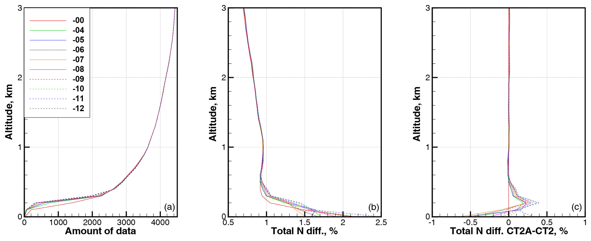
Figure 9Statistics for latitude band 60–70∘. (a) Amount of data. (b) RMS relative difference in refractivity COSMIC–ECMWF ΔNCE. (c) RMS relative difference in refractivity CT2A–CT2. All are functions of the parameter β.
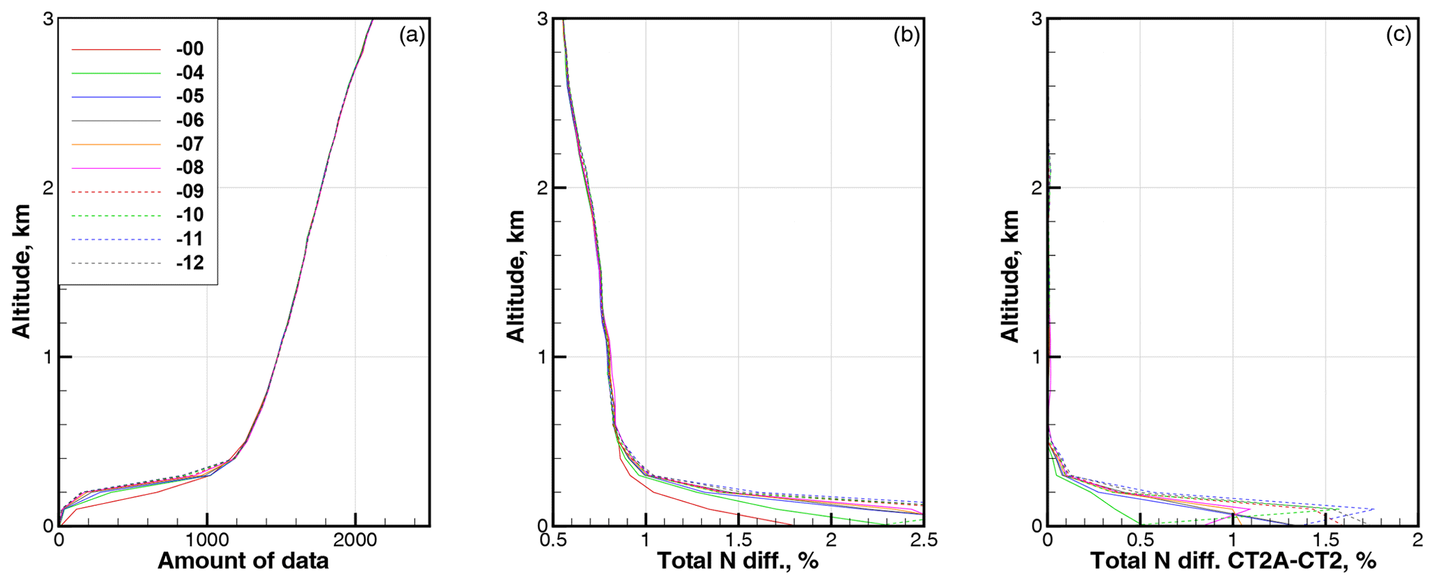
Figure 10Statistics for latitude band 70–80∘. (a) Amount of data. (b) RMS relative difference in refractivity COSMIC–ECMWF ΔNCE. (c) RMS relative difference in refractivity CT2A–CT2. All are functions of the parameter β.

Figure 11Statistics for latitude band 80–90∘. (a) Amount of data. (b) RMS relative difference in refractivity COSMIC–ECMWF ΔNCE. (c) RMS relative difference in refractivity CT2A–CT2. All are functions of the parameter β.
The statistics for different β, presented in the above figures, was evaluated independently, i.e., the statistical ensembles were different. Figures 12 and 13 show the statistics for the common datasets including events passing QC for both β=0 and current values of β. The statistical differences between refractivity retrieved with β=0 and other values of β are indistinguishably small (never exceeding a level of 0.0005 %). Here the reduction of ΔNCE is slightly more than in Figs. 3 and 4
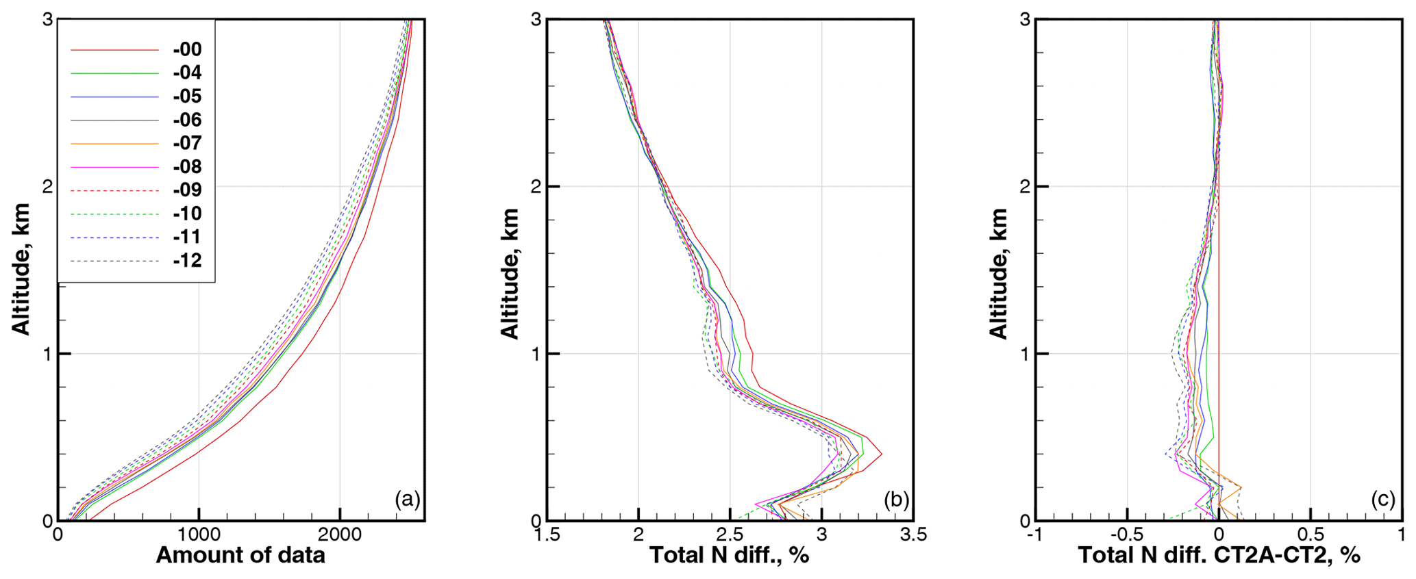
Figure 12Statistics for latitude band 0–10∘ evaluated for subsets common for β=0 and each other value of β. (a) Amount of data. (b) RMS relative difference in refractivity COSMIC–ECMWF ΔNCE. (c) RMS relative difference in refractivity CT2A–CT2. All are functions of the parameter β.
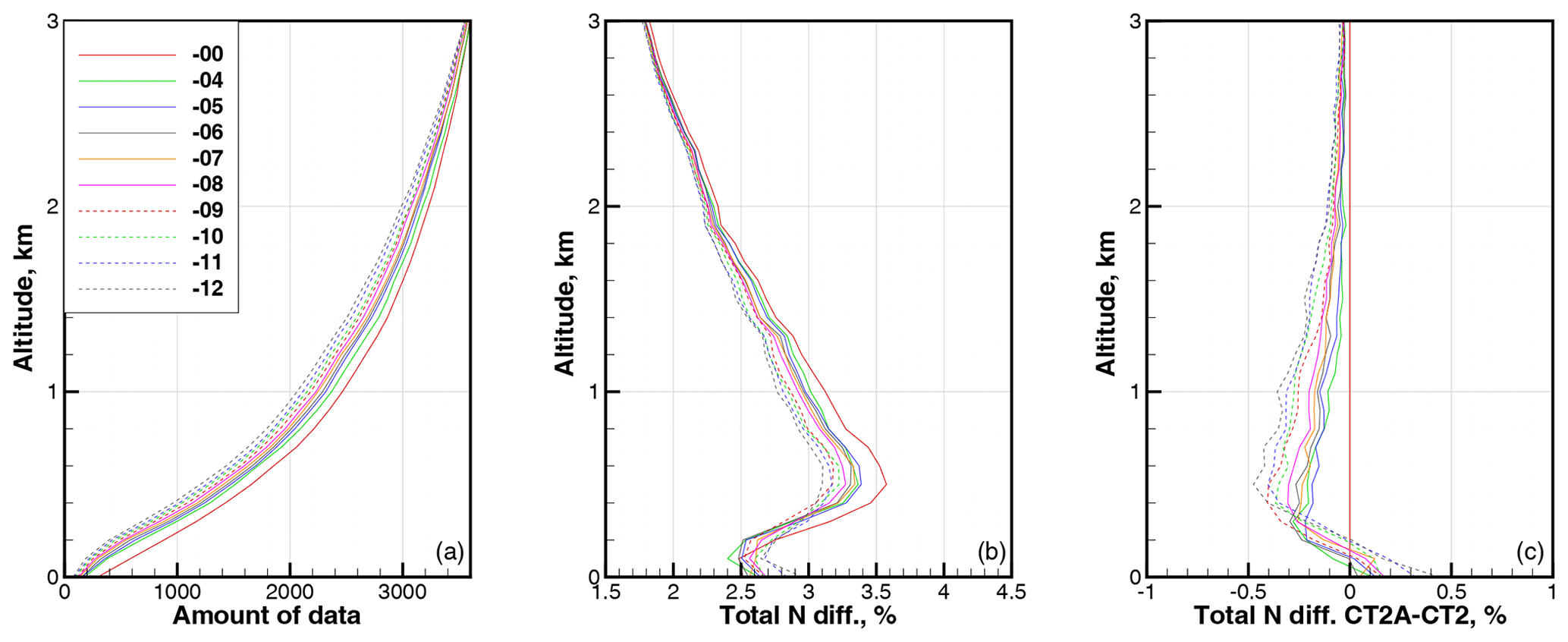
Figure 13Statistics for latitude band 10–20∘ evaluated for subsets common for β=0 and each other value of β. (a) Amount of data. (b) RMS relative difference in refractivity COSMIC–ECMWF ΔNCE. (c) RMS relative difference in refractivity CT2A–CT2. All are functions of the parameter β.
This indicates that CT2A acts as a QC procedure not involving any external data and only based on the internal properties of observed signals. On average, CT2A provides a higher cut-off height which is estimated from the CT amplitude by correlating it with the θ function (Gorbunov et al., 2006). By looking at the ray manifold in the phase space from different directions, it is possible to choose ray manifold pieces where its structure is most stable.
In this study, we discussed the general idea of the canonical transform (CT) method and provided a new generalization adding more flexibility for application in RO processing. CTs in classical mechanics (geometrical optics) are implemented in quantum mechanics (wave optics) by linear operators with oscillating kernels. Such operators are referred to as Fourier integral operators (FIOs). During the past century, this approach acquired a solid theoretical basis. In numerous mathematical monographs, one finds the advanced theory of FIOs. The central role in this theory is played by the concept of the ray manifold and its projections.
In quantum mechanics and wave optics, FIOs were employed for the quantization procedure, i.e., the construction of the asymptotic quantum (quasi- or semiclassical) solutions on the basis of the classical (geometric optical) ones. The idea of the CT method for processing RO observations is the reverse: the reconstruction of the geometric optical solution from the wave optical one, which can be referred to as the dequantization.
Although there have been many modifications, like original CT combined with back propagation (BP), full spectrum inversion (FSI), phase matching (PM), and CT of type 2 (CT2), there is no essential difference between these FIO-based methods. The difference consists of the approximation of the phase function of the FIO leading to the corresponding approximate representation of the impact parameter and bending angle and in the specific implementation (such as cut-off, filtering, and quality control procedures). All these methods map the wave field into the representation of the impact parameter p. This choice of the coordinate in the mapped space has its reasons: in the case of a spherically symmetric medium, the impact parameter is always a unique coordinate of the ray manifold.
The implementation of this idea in the real, non-spherically symmetric atmosphere encounters some difficulties. First, in the strict sense, there is no such quantity as the impact parameter as a unique variable any more, but it is still possible to operate with the effective impact parameter derived from Doppler frequency shift using the same relations as for a spherically symmetric medium. This quantity can be implemented in the observation operator for the variational assimilation of RO observations, canceling errors due to horizontal gradients. However, the above property of the impact parameter, which is supposed to be a unique coordinate of the ray manifold, does not always hold for the effective value. In some cases, the situation referred to as the impact parameter multipath may occur, resulting in retrieval errors in atmospheric profiles derived from RO data.
In order to mitigate this fundamental shortcoming, we introduced a generalization of the CT approach. We used a generalized definition of the coordinate in phase space, defined as a linear combination of the impact parameter and bending angle. Because this can be understood as an affine transform of the phase space, we coined the abbreviation CT2A for the new method. This transform has a parameter β which can be tuned to optimize the algorithm's performance.
We implemented the CT2A algorithm by modifying our existing program code for the CT2 method. In order to evaluate its statistical performance under real RO observation conditions, including challenging horizontal gradients in the lower troposphere, we processed a large ensemble of COSMIC RO data for the year 2008 on the 1st and 15th day of every month, adding up to a total of about 60 000 RO events. We used the total relative difference in COSMIC from collocated ECMWF analysis profiles over the lower troposphere as the metric for this evaluation and the tuning parameter estimation.
For the latitudes of 0–30∘ and for the altitudes between 0.4 and 2.5 km, the application of the CT2A algorithm decreased the COSMIC–ECMWF difference metric with increasing parameter β. For the altitudes below 0.4 km, the optimal value of parameter β is found to be −4 to −9 km/rad. This was achieved on account of a slight decrease in the amount of data passing through the whole retrieval chain including the QC. This indicates that the CT2A itself implements a QC procedure that does not involve any external information about the atmospheric refractivity but is only based on the analysis of the structure of the observed signals.
Overall, these results suggest that the CT2A method is not only theoretically an innovative generalization of the CT or FIO class of methods but also practically a valuable advancement for RO processing in that it can improve the capability to cope with challenging horizontal gradient conditions in the lower troposphere and serve as the basis of a new QC procedure.
The COSMIC data used in this study are freely available at CDAAC website.
KBL formulated the problem, introduced the initial idea of the study, participated in theoretical discussions, and contributed to finalizing the paper. MG performed the theoretical derivations, implemented the algorithm numerically, performed the statistical study, and wrote the initial draft of the paper. GK participated in theoretical discussions and contributed to finalizing the paper.
The authors declare that they have no conflict of interest.
Michael Gorbunov is grateful for the Russian Foundation for Basic Research (grant no. 20-05-00189 A) for the financial support. Gottfried Kirchengast acknowledges support, including partial co-funding of the work of Michael Gorbunov, from the Aeronautics and Space Agency of the Austrian Research Promotion Agency (FFG-ALR) under the Austrian Space Applications Programme (ASAP) project ATROMSAF1 (proj. no. 859771) funded by the Ministry for Transport, Innovation, and Technology (BMVIT). Kent B. Lauritsen has been supported by the Radio Occultation Meteorology Satellite Application Facility (ROM SAF), which is a decentralized operational RO processing center under EUMETSAT. The authors acknowledge Taiwan’s National Space Organization (NSPO) and the University Corporation for Atmospheric Research (UCAR) for providing the COSMIC data.
This research has been supported by the Russian Foundation for Basic Research (grant no. 20-05-00189) and the Aeronautics and Space Agency of the Austrian Research Promotion Agency (grant no. 859771).
This paper was edited by Peter Alexander and reviewed by two anonymous referees.
Arnold, V. I.: Mathematical Methods of Classical Mechanics, Springer, New York, USA, 1978. a, b, c, d, e, f, g
Egorov, Y. V.: Lectures on Partial Differential Equations, Moscow State University Press, Moscow, Russia, 1985 (in Russian). a, b, c, d
Egorov, Y. V. and Shubin, M. A.: Partial Differential Equations IV, Springer, Berlin and Heidelberg, Germany, https://doi.org/10.1007/978-3-662-09207-1, 1993. a, b, c, d
Fock, V. A.: Fundamentals of Quantum Mechanics, Mir Publishers, available at: https://archive.org/details/FockFundamentalsOfQuantumMechanicsMir1986 (last access: 22 January 2021), 1978. a, b, c, d, e, f
Goldstein, H., Poole, C., and Safko, J.: Classical Mechanics, Pearson Education Limited, London, UK, 2014. a, b, c, d, e, f
Gorbunov, M. E.: Canonical transform method for processing radio occultation data in the lower troposphere, Radio Sci., 37, 1076, https://doi.org/10.1029/2000RS002592, 2002. a, b, c, d, e
Gorbunov, M. E. and Gurvich, A. S.: Microlab-1 experiment: Multipath effects in the lower troposphere, J. Geophys. Res., 103, 13819–13826, https://doi.org/10.1029/98JD00806, 1998a. a, b
Gorbunov, M. E. and Gurvich, A. S.: Algorithms of inversion of Microlab-1 satellite data including effects of multipath propagation, Int. J. Remote Sens., 19, 2283–2300, https://doi.org/10.1080/014311698214721, 1998b. a, b
Gorbunov, M. E. and Kornblueh, L.: Analysis and validation of GPS/MET radio occultation data, J. Geophys. Res., 106, 17161–17169, https://doi.org/10.1029/2000JD900816, 2001. a, b, c, d
Gorbunov, M. E. and Lauritsen, K. B.: Canonical Transform Methods for Radio Occultation Data, Scientific Report 02-10, Danish Meteorological Institute, Copenhagen, Denmark, available at: http://www.romsaf.org/Publications/reports/sr02-10.pdf (last access: 22 January 2021), 2002. a
Gorbunov, M. E. and Lauritsen, K. B.: Analysis of wave fields by Fourier integral operators and its application for radio occultations, Radio Sci., 39, RS4010, https://doi.org/10.1029/2003RS002971, 2004a. a, b, c, d, e, f, g, h, i
Gorbunov, M. E. and Lauritsen, K. B.: Canonical Transform Methods for Radio Occultation Data, in: Occultations for Probing Atmosphere and Climate, edited by: Kirchengast, G., Foelsche, U., and Steiner, A. K., Springer, Berlin and Heidelberg, Germany, 61–68, https://doi.org/10.1007/978-3-662-09041-1_6, 2004b. a, b
Gorbunov, M. E. and Lauritsen, K. B.: Error Estimate of Bending Angles in the Presence of Strong Horizontal Gradients, in: New Horizons in Occultation Research, edited by: Steiner, A., Pirscher, B., Foelsche, U., and Kirchengast, G., Springer, Berlin and Heidelberg, Germany, 17–26, https://doi.org/10.1007/978-3-642-00321-9_2, 2009. a, b, c, d, e
Gorbunov, M. E., Gurvich, A. S., and Bengtsson, L.: Advanced Algorithms of Inversion of GPS/MET Satellite Data and their Application to Reconstruction of Temperature and Humidity, Report No. 211, Max-Planck Institute for Meteorology, Hamburg, Germany, available at: https://www.mpimet.mpg.de/en/science/publications/archive/mpi-reports-1987-2004/ (last access: 22 January 2021), 1996a. a, b
Gorbunov, M. E., Sokolovskiy, S. V., and Bengtsson, L.: Space Refractive Tomography of the Atmosphere: Modeling of Direct and Inverse Problems, Report No. 210, Max-Planck Institute for Meteorology, Hamburg, Germany, https://www.mpimet.mpg.de/fileadmin/publikationen/Reports/MPI-Report_210.pdf (last access: 22 January 2021), 1996b. a
Gorbunov, M. E., Benzon, H.-H., Jensen, A. S., Lohmann, M. S., and Nielsen, A. S.: Comparative analysis of radio occultation processing approaches based on Fourier integral operators, Radio Sci., 39, RS6004, https://doi.org/10.1029/2003RS002916, 2004. a
Gorbunov, M. E., Lauritsen, K. B., Rhodin, A., Tomassini, M., and Kornblueh, L.: Radio holographic filtering, error estimation, and quality control of radio occultation data, J. Geophys. Res., 111, D10105, https://doi.org/10.1029/2005JD006427, 2006. a
Gorbunov, M. E., Shmakov, A. V., Leroy, S. S., and Lauritsen, K. B.: COSMIC Radio Occultation Processing: Cross-center Comparison and Validation, J. Atmos. Oceanic Tech., 28, 737–751, https://doi.org/10.1175/2011JTECHA1489.1, 2011. a
Gorbunov, M., Stefanescu, R., Irisov, V., and Zupanski, D.: Variational Assimilation of Radio Occultation Observations into Numerical Weather Prediction Models: Equations, Strategies, and Algorithms, Remote Sens., 11, 2886, https://doi.org/10.3390/rs11242886, 2019. a, b
Healy, S. B.: Radio occultation bending angle and impact parameter errors caused by horizontal refractive index gradients in the troposphere: A simulation study, J. Geophys. Res., 106, 11875–11890, https://doi.org/10.1029/2001JD900050, 2001. a, b
Hörmander, L.: The Analysis of Linear Partial Differential Operators, vol. III, Pseudo-Differential Operators, Springer, New York, USA, 1985a. a, b, c
Hörmander, L.: The Analysis of Linear Partial Differential Operators, vol. IV, Fourier Integral Operators, Springer, New York, USA, 1985b. a, b, c
Jensen, A. S., Lohmann, M. S., Benzon, H.-H., and Nielsen, A. S.: Full spectrum inversion of radio occultation signals, Radio Sci., 38, 1–15, https://doi.org/10.1029/2002RS002763, 2003. a, b, c
Jensen, A. S., Lohmann, M. S., Nielsen, A. S., and Benzon, H.-H.: Geometrical optics phase matching of radio occultation signals, Radio Sci., 39, RS3009, https://doi.org/10.1029/2003RS002899, 2004. a, b, c
Karayel, T. E. and Hinson, D. P.: Sub-Fresnel scale resolution in atmospheric profiles from radio occultation, Radio Sci., 32, 411–423, https://doi.org/10.1029/96RS03212, 1997. a, b
Kursinski, E. R., Hajj, G. A., Schofield, J. T., Linfield, R. P., and Hardy, K. R.: Observing Earth's atmosphere with radio occultation measurements using the Global Positioning System, J. Geophys. Res., 102, 23429–23465, https://doi.org/10.1029/97JD01569, 1997. a, b
Melbourne, W. G., Davis, E. S., Duncan, C. B., Hajj, G. A., Hardy, K. R., Kursinski, E. R., Meehan, T. K., and Young, L. E.: The Application of Spaceborne GPS to Atmospheric Limb Sounding and Global Change Monitoring, Jet Propulsion Laboratory, Pasadena, CA, USA, 1994. a
Mishchenko, A. S., Shatalov, V. E., and Sternin, B. Y.: Lagrangian manifolds and the Maslov operator, Springer, Berlin, Germany and New York, USA, 1990. a
Mortensen, M. D. and Høeg, P.: Inversion of GPS occultation measurements using Fresnel diffraction theory, Geophys. Res. Lett., 25, 2441–2444, https://doi.org/10.1029/98GL51838, 1998. a
Treves, F.: Introduction to Pseudodifferential Operators and Fourier Integral Operators, vol. 1, Pseudodifferential Operators, Plenium Press, New York, USA and London, UK, 1982a. a, b, c
Treves, F.: Introduction to Pseudodifferential Operators and Fourier Integral Operators, vol. 2, Fourier Integral Operators, Plenium Press, New York USA, and London, UK, 1982b. a, b, c
Ware, R., Exner, M., Feng, D., Gorbunov, M., Hardy, K., Herman, B., Kuo, Y.-H., Meehan, T., Melbourne, W., Rocken, C., Schreiner, W., Sokolovsky, S., Solheim, F., Zou, X., Anthes, R., Businger, S., and Trenberth, K.: GPS Sounding of the Atmosphere from Low Earth Orbit: Preliminary Results, B. Am. Meteorol. Soc., 77, 19–40, https://doi.org/10.1175/1520-0477(1996)077<0019:GSOTAF>2.0.CO;2, 1996. a, b
Zou, X., Liu, H., and Anthes, R. A.: A Statistical Estimate of Errors in the Calculation of Radio-Occultation Bending Angles Caused by a 2D Approximation of Ray Tracing and the Assumption of Spherical Symmetry of the Atmosphere, J. Atmos. Ocean. Tech., 19, 51–64, https://doi.org/10.1175/1520-0426(2002)019<0051:ASEOEI>2.0.CO;2, 2002. a
Zou, X., Liu, H., and Kuo, Y.-H.: Occurrence and detection of impact multipath simulations of bending angle, Q. J. Roy. Meteor. Soc., 145, 1690–1704, https://doi.org/10.1002/qj.3520, 2019. a, b, c, d
- Abstract
- Introduction
- General concept of canonical transform in wave optics
- The canonical transform method for RO and its generalization
- Implementation and numerical performance evaluation
- Summary and conclusions
- Data availability
- Author contributions
- Competing interests
- Acknowledgements
- Financial support
- Review statement
- References