the Creative Commons Attribution 4.0 License.
the Creative Commons Attribution 4.0 License.
 | 05 Feb 2021
Flywheel calibration of a continuous-wave coherent Doppler wind lidar
Anders Tegtmeier Pedersen
Michael Courtney
A rig for calibrating a continuous-wave coherent Doppler wind lidar has been constructed. The rig consists of a rotating flywheel on a frame together with an adjustable lidar telescope. The laser beam points toward the rim of the wheel in a plane perpendicular to the wheel's rotation axis, and it can be tilted up and down along the wheel's periphery and thereby measure different projections of the tangential speed. The angular speed of the wheel is measured using a high-precision measuring ring fitted to the periphery of the wheel and synchronously logged together with the lidar speed. A simple geometrical model shows that there is a linear relationship between the measured line-of-sight speed and the beam tilt angle, and this is utilised to extrapolate to the tangential speed as measured by the lidar. An analysis of the uncertainties based on the model shows that a standard uncertainty on the measurement of about 0.1 % can be achieved, but also that the main source of uncertainty is the width of the laser beam and its associated uncertainty. Measurements performed with different beam widths confirm this. Other measurements with a minimised beam radius show that the method in this case performs about equally well for all the tested reference speeds ranging from about 3 to 18 m s−1.
- Article
(3731 KB) - Full-text XML
- BibTeX
- EndNote


Wind lidars are often referred to as being “absolute” instruments which means that, given only the parameters of the laser wavelength and the frequency at which we sample the backscattered light, we are able to calculate the measured line-of-sight (LOS) speed through the well-known equation (Pearson et al., 2002). This to some extent implies that wind lidars are also “calibration free” since, in contrast to, e.g. cup anemometers, there are no empirical constants to be found through a calibration. However, a calibration is fundamentally just a comparison to a reference with a known and traceable uncertainty (Joint Committee for Guides in Metrology, 2012), and without a calibration we have no way of knowing that the lidar measures correctly; small errors can easily creep into the frequency analysis or the laser wavelength may drift, etc. It is equally important that, by using a reference with known uncertainty traceable to international measurement prototypes, we can assign an uncertainty to the lidar radial speed and claim traceability. The latter is often a requirement in commercial measurements where the outcome can have financial consequences. The uncertainty of the calibration can further be transferred to the test instrument and form the basis for additional operational uncertainty estimates.
The current practice for calibrating wind lidars is to use cup or sonic anemometers (Courtney, 2013) as a reference instrument, and the calibration is often limited by the uncertainty of the reference instrument. Even when using sonic anemometers as the reference, the overall lidar calibration uncertainty is typically of the order of 1 %–2 % (Wagenaar et al., 2016). This does not do justice to the lidars. We believe that the potential accuracy of wind lidars is much higher than that (lasers are after all very stable instruments and frequency analysis not necessarily faulty), and therefore we propose a new calibration method with a targeted standard uncertainty of 0.1 %. The result of such an order of magnitude increase in accuracy can hopefully propagate through the wind energy industry as higher accuracy will have significant economic benefits.
Inspired by a similar concept commonly used for calibrating laser Doppler anemometers (LDAs) (Shinder et al., 2013), we have constructed a rig for calibrating Doppler lidars. The rig in essence consists of a frame with a stainless-steel flywheel on one end and an adjustable lidar telescope pointing toward the wheel rim on the other. However, conversely to an LDA system, a Doppler lidar measures the velocity component along the laser beam, and we therefore use the lidar beam skimming on the circumference rather than impinging the wheel surface perpendicularly as the LDA would do. The telescope is mounted on a pivoting mechanism, and with this the laser beam can be tilted and thus different projections of the wheel peripheral speed probed. In addition, we have developed a simple model relating the ratio between the speed sensed by the lidar and the peripheral speed to the beam tilt angle, and this method allows us to estimate the true peripheral speed by extrapolation from speeds measured at other angles.
It might seem strange to use a rotating steel wheel as the measurement target; after all, the lidar is intended for measuring small aerosols carried by the wind and not a solid metal target. On the other hand, the lidar fundamentally measures a frequency shift in the backscattered light due to a relative motion, and it is this frequency shift measurement and the subsequent conversion to a speed we wish to calibrate. The origin of the backscatter is, in this connection, of less importance. One could, however, envision a scenario where a lidar calibrated in this fashion is used to calibrate another lidar, e.g. in a wind tunnel or the free atmosphere. This would lead to a calibration procedure resembling that of the current practice but where the limiting accuracy of a cup anemometer is alleviated.
The paper is organised in the following way. First, the calibration rig and lidar are described. Then the model describing the relation between the measured line-of-sight speed and tilt angle is gradually developed, beginning from a simple 1-D model to a more realistic 2-D model and finally a 3-D model. This model forms the basis of the following suggestion for a calibration procedure and analysis of the various uncertainty contributions. Finally, calibrations performed with different laser beam widths and at different reference speeds are presented.
The calibration rig consists of an aluminium frame on which a stainless-steel wheel is mounted together with the transceiver, or telescope, of the lidar. The wheel has a radius of 286.76 mm with a measured eccentricity of about 0.01 mm, and it is coupled directly to a servo motor to control its rotational speed. The telescope is mounted at approximately the same height as the top of the wheel and in such a way that it can be tilted around a horizontal axis parallel to the wheel's rotational axis using a fine-threaded adjustment screw; see Fig. 1. The pivot point is located approximately 10 cm directly under the lens. An inclinometer is mounted on top of the telescope to measure the tilt angle of the laser beam.
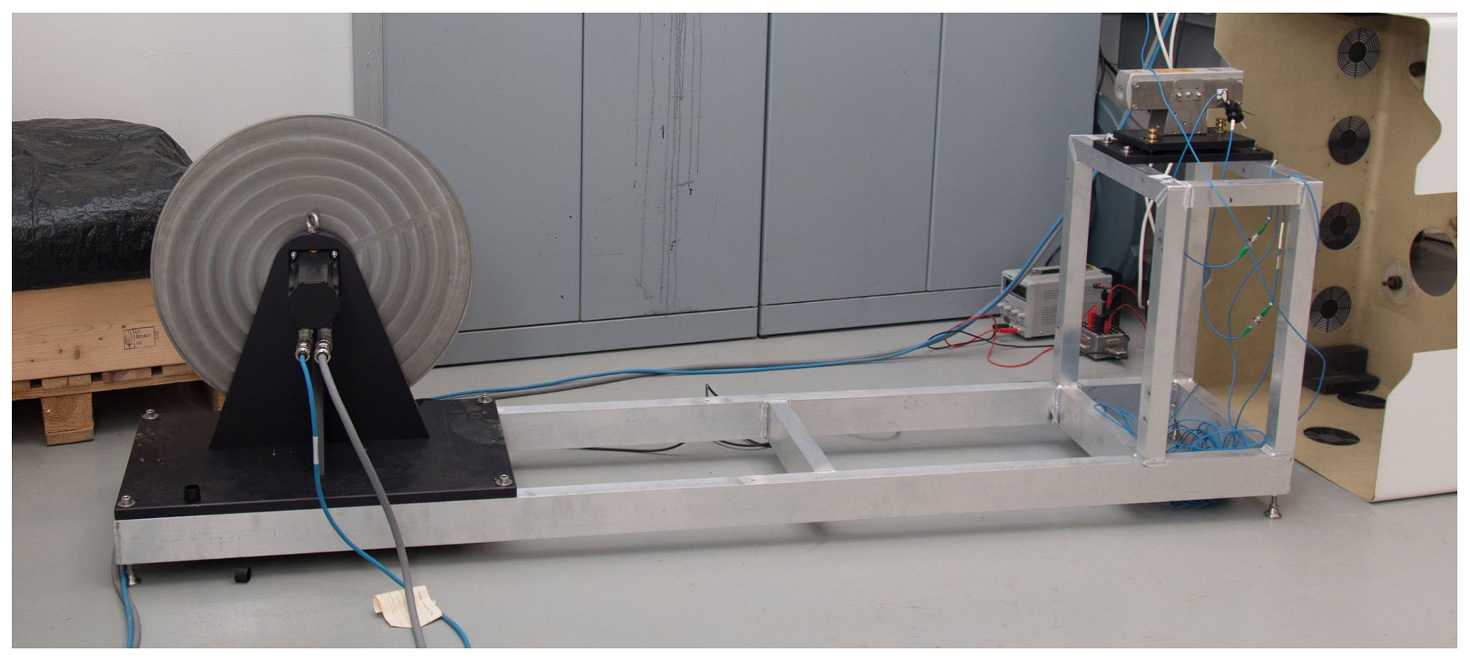
Figure 1Photo of the calibration rig. To the left is the flywheel with cables through which the motor is controlled and to the right the lidar telescope with optical cables connecting it with the laser and detectors. The inclinometer is not visible in the photo.
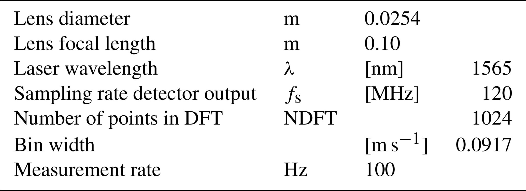
In order to measure the rotational speed, a high-precision measuring ring is fitted to the periphery of the wheel together with a corresponding measurement head sitting near the bottom of the wheel (AMO GmbH, 2013). As the wheel rotates, the ring induces a voltage in the static measurement head for each 1000 µm ± 3 µm. The output of the system is 1800 TTL (transistor–transistor logic) pulses per wheel revolution, and the period for six consecutive pulses is measured and inverted to give the wheel rotational frequency. The physical properties of the calibration rig are summarised in Table 1.

The lidar is a direction sensitive continuous-wave coherent Doppler lidar operated with a 1565 nm fibre laser (Pedersen et al., 2014). The Doppler spectra are based on a 1024-point discrete Fourier transform (DFT) of the detector output sampled at 120 MHz resulting in a spectrum resolution of 117 kHz or 0.0917 m s−1. About 1200 spectra are combined to form one average spectrum at a rate of approximately 100 Hz. Based on the average spectrum, the radial speed is estimated as the 50 % fractile of the signal exceeding the detection threshold (Angelou et al., 2012). Focusing of the laser beam is controlled by adjusting the distance from the laser output fibre to the focusing lens with a micrometre screw. The lens has a 1 in diameter and a focal length of 0.10 m. The laser, telescope and detectors are connected by optical fibres. The physical properties of the lidar are summarised in Table 2.
Real-time signals from lidar, inclinometer and rotation encoder are streamed to a measurement computer which synchronises at 100 Hz and stores the data for post-processing.
A rotating wheel for calibration has been used with LDAs for many years (Shinder et al., 2013; Bean and Hall, 1999; Duncan and Keck, 2009), and as mentioned in Sect. 1, our calibration rig is strongly inspired by what has been done with LDAs. However, unlike LDAs, coherent Doppler lidars measure the velocity component along the laser beam, meaning that the beam must be aligned with and overlapping a tangent of the wheel. This poses a paradox since for the lidar to measure the true tangential wheel speed, and only that, the overlap between laser beam and wheel surface will need to be infinitely small. In this case, there will be no backscatter signal to detect! In order to circumvent this paradox, it is therefore necessary to measure a different component of the reference speed than the tangential together with the corresponding tilt angle and from that calculate the measured tangential speed. Unfortunately, this approach also has some drawbacks in the form of additional uncertainties due to the tilt angle measurement. Another source of uncertainty, present at any tilt angle, is the speed estimation uncertainty due to the finite resolution of the measured Doppler spectrum, which is especially pronounced when using a very narrow laser beam. The narrow beam leads to only a very limited range of projected speeds being sensed confining the Doppler signal to a single spectral bin. However, this uncertainty can be eliminated by scanning over a range of tilt angles or, alternatively, a range of wheel speeds. We have developed a model from simple geometric considerations describing the ratio between the tangential wheel speed and the speed sensed by the lidar as a function of beam tilt angle. The model shows that this relationship is linear, and it can therefore be used to make a simple extrapolation back to what would be the tangential wheel speed sensed by the lidar.
In the following subsections, the model is derived: first under the approximation that the laser beam has no transverse component (i.e. it is infinitely narrow), during which we establish the relationship between the beam tilt angle, θ, and the skimming angle, ϕs, and later for a collimated beam of finite width, w. The model predicts that there are two distinct measurement regimes: one when the entire beam is on the wheel and one when part of the laser beam skims above the wheel, and this has a profound influence on interpreting the result. Finally, the suggested procedure for doing the calibration is described.
3.1 Infinitely narrow beam
Figure 2 shows a schematic drawing of the calibration setup. The line-of-sight speed sensed by the lidar (VLOS) is the wheel's peripheral velocity projected into the direction of the beam at the point of intersection between the wheel surface and laser beam. From Fig. 2, this is seen to be
where Vwheel is the peripheral speed, ϕs is the skimming angle, θ is the beam tilt angle, ω is the angular frequency, and R is the radius of the wheel.
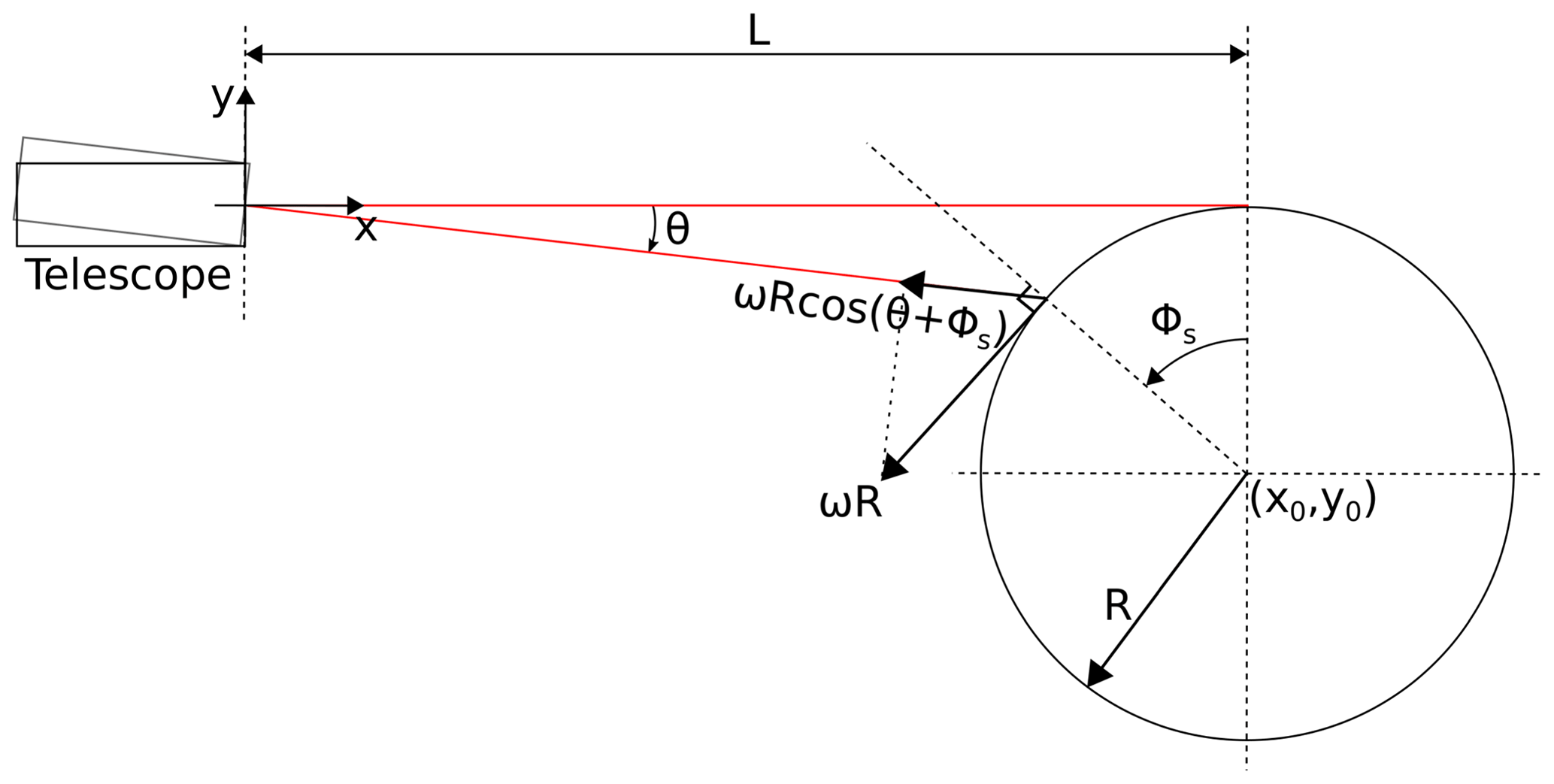
Figure 2Schematic drawing of the calibration rig illustrating the basic geometry of the rig. The laser beam, illustrated in red, can be tilted using an adjustment screw on the telescope mount.
Now, to find the relation between ϕs and θ, we can make use of an approach which will also prove valuable later on; instead of tilting the beam, we rotate the centre of the wheel, (x0,y0), an angle θ around the centre of the transceiver lens which defines the origin of our coordinate system; see Fig. 3. The new centre of the wheel is denoted (xr,yr). From the figure, it is clear that the angle, ϕr, between the vertical and the intersection point between beam and wheel is
and that
From Fig. 2, we see that (x0,y0)=(), and from this we can calculate (xr,yr) via the rotation matrix Rz(θ)
As mentioned in Sect. 2, the physical beam actually rotates around a point situated beneath the lens, but for a tilt angle of 2.5∘, which is the maximum attainable in our setup, this leads to a negligible difference for xr and yr of about 4 and 0.1 mm, respectively. Now, rearranging and inserting into Eq. (1), we finally arrive at
Since the maximum tilt angle is only about 2.5∘, we can make the approximations that cos θ=1 and sin θ=θ such that
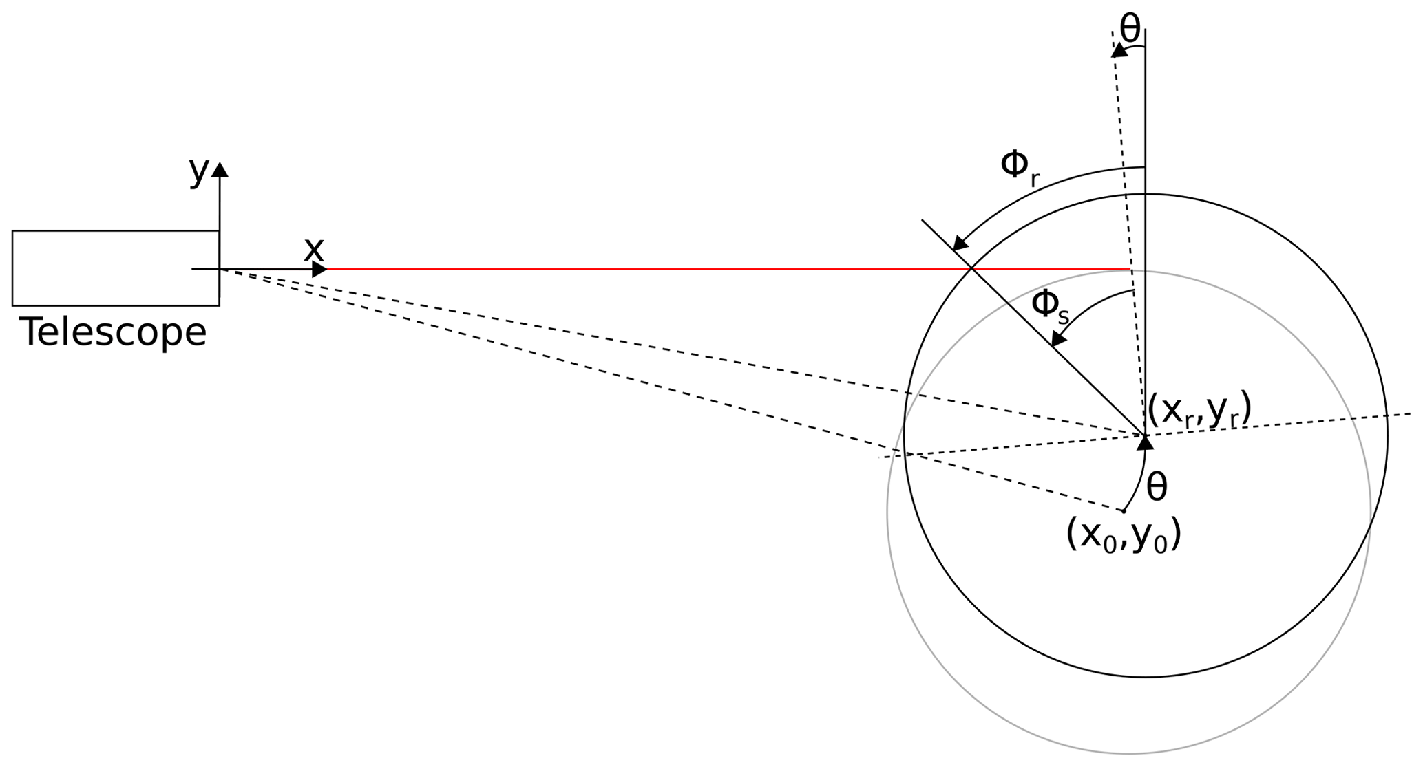
Figure 3Instead of tilting the beam, the centre of the wheel is rotated around the lens centre.
It is thus seen that for small tilt angles there is a linear relationship between the speed ratio and θ, and this can be utilised in the calibration procedure.
3.2 Finite width, collimated beam, 2-D
Now, a real laser beam is of course not infinitely narrow but has a transverse profile of finite width; e.g. the laser used in this study has a Gaussian profile. We therefore expand the model to include the beam width radius, w, but to begin with, limit ourselves to the two-dimensional case and the assumption that the beam intensity has a constant transverse cross section; i.e. the intensity profile across the beam has a “top-hat shape”.
For a beam of finite width, a finite part of the wheel perimeter will be illuminated by the laser and thus a range of line-of-sight speeds be measured; see Fig. 4. Each incremental line-of-sight speed will be
and these will each contribute a proportion d of the total speed sensed by the lidar, where is the total angle subtended by lidar illumination. The total speed contribution VLOS is thus obtained by integrating Eq. (7) whilst normalising by Δϕr:
By applying L'Hospital's rule, the right-hand side divided by Vwheel is easily seen to reduce to cos ϕr as approaches , i.e. as the beam becomes narrower, and therefore give the same result as in Sect. 3.1, and the model is thus mathematically consistent with the 1-D model.
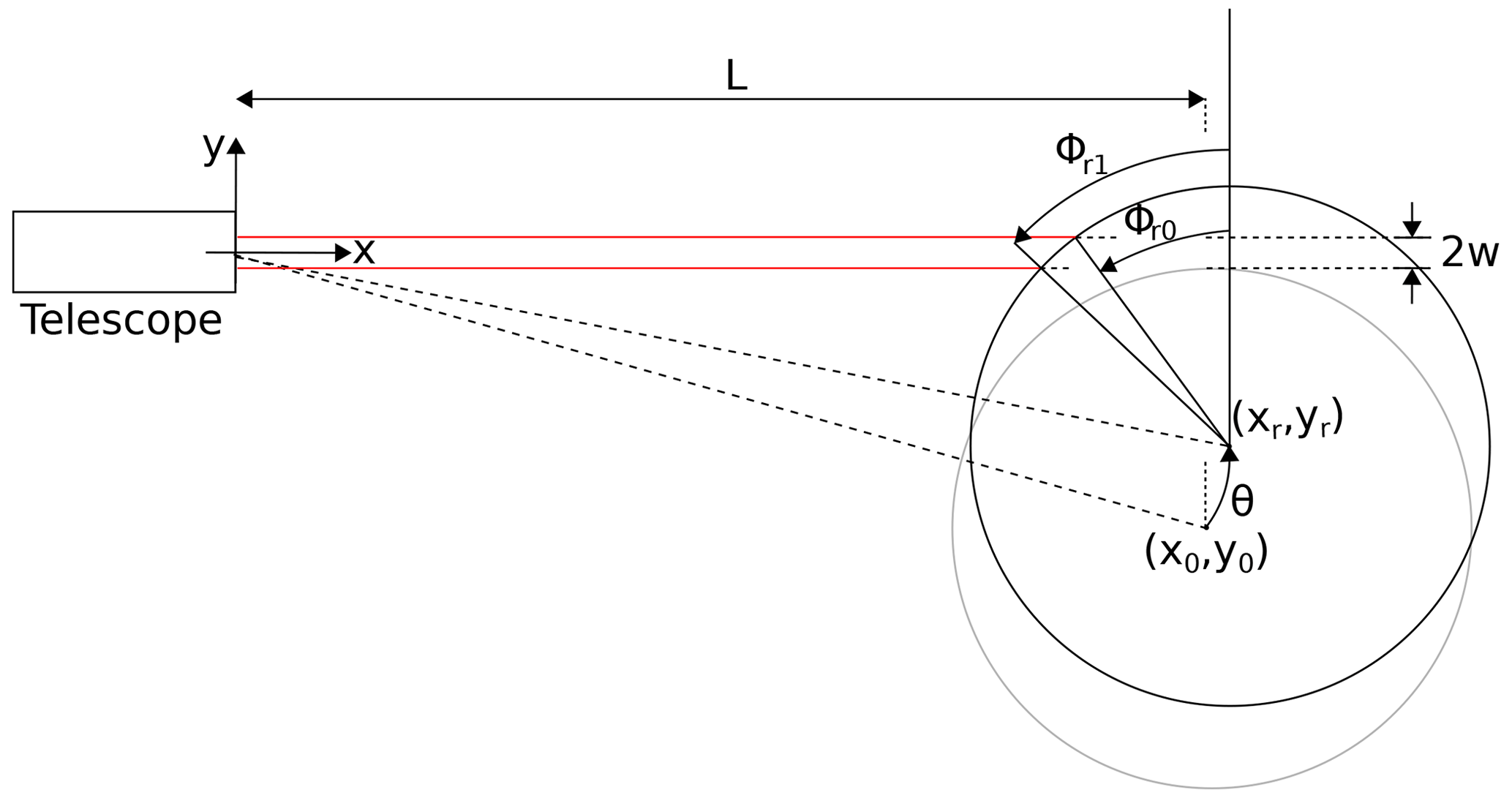
Figure 4Schematic drawing used to derive the 2-D thick beam model. Notice that w is the beam radius and ().
Even for a beam of finite width, Eq. (6) is a good approximation to how the ratio changes as the beam is tilted. For completeness, a mathematical derivation of this is presented in Appendix A, but from a physical point of view it can intuitively be understood as that the high speed measured at ϕ1 is more or less balanced by the low speed measured at ϕ0. However, the approximation only applies as long as the entire beam cross section is on the wheel; if part of the beam goes above the wheel, as it will for very small tilt angles, the relationship changes, as we shall see in Sect. 3.2.1.
3.2.1 Skimming above the wheel
As mentioned above, Eq. (6) only applies as long as all of the beam is on the wheel, but if parts of the beam go above the wheel the relationship between and θ changes, and this is unavoidably what will happen when we try to measure as close as possible to the true tangential speed. It is therefore interesting to take a closer look at the special case characterised by ϕ0=0, that is, for such small tilt angles that only parts of the beam hit the wheel. Furthermore, measuring in this angular range can be used to estimate the beam width which will be explained in Sect. 3.6: when skimming above the wheel, Eq. (8) reduces to
and if we Taylor expand, we get
This means that as long as only a part of the beam is impinging on the wheel the sensitivity to the tilt angle is only a third compared to when the entire beam illuminates the wheel. The range of angles to which this applies obviously depends on the beam width. The angle where the top of the beam first touches the wheel, i.e. when the entire beam is on the wheel, is denoted θ1 and is calculated through
3.3 3-D model
In the previous section, we modelled the laser beam intensity profile as a 2-D top-hat shape. This is in conflict with the physical reality in two ways; firstly, confining the model to two dimensions effectively means that we are assuming the beam cross section to be square and not round, and secondly the real laser beam has a Gaussian intensity profile and not a top-hat shape. To take these facts into account, we must therefore expand the model to three dimensions.
Still assuming that the beam is collimated, we can model the beam as a cylinder of radius w centred around the x axis:
and the wheel as a cylinder along the z axis and centred around (xr,yr):
The x coordinates of the overlap between beam and wheel in the rotated frame of reference are found by solving Eq. (13):
where , and the sign of the square root is chosen such that only parts of the wheel facing the telescope are illuminated. The corresponding y and z coordinates are governed by Eq. (12) such that (). It should be noticed that in this way the overlap between wheel and beam has been parameterised into a function of y and z, i.e. ).
In order to find the ratio , we follow the same procedure as outlined in Sect. 3.2 by integrating all the speed contributions and normalise by the area of the illuminated surface, S. This can be done by calculating the surface integrals:
where I(y,z) is the beam intensity profile. The full derivation of Eq. (15) can be found in Appendix B.
3.4 Model comparison
In order to compare the different models from the simple narrow beam approximation and 2-D top-hat beam to the full 3-D Gaussian beam, a numerical evaluation of each has been performed for a beam radius of 2.5 mm ( radius for the Gaussian profile) and plotted together as a function of tilt angle in Fig. 5. The left plot shows the models evaluated from θ=0–1∘ and the right is a close-up focusing on the transition range where more and more of the beam falls on the wheel. The values used for R and L are the same as those for the actual calibration rig.
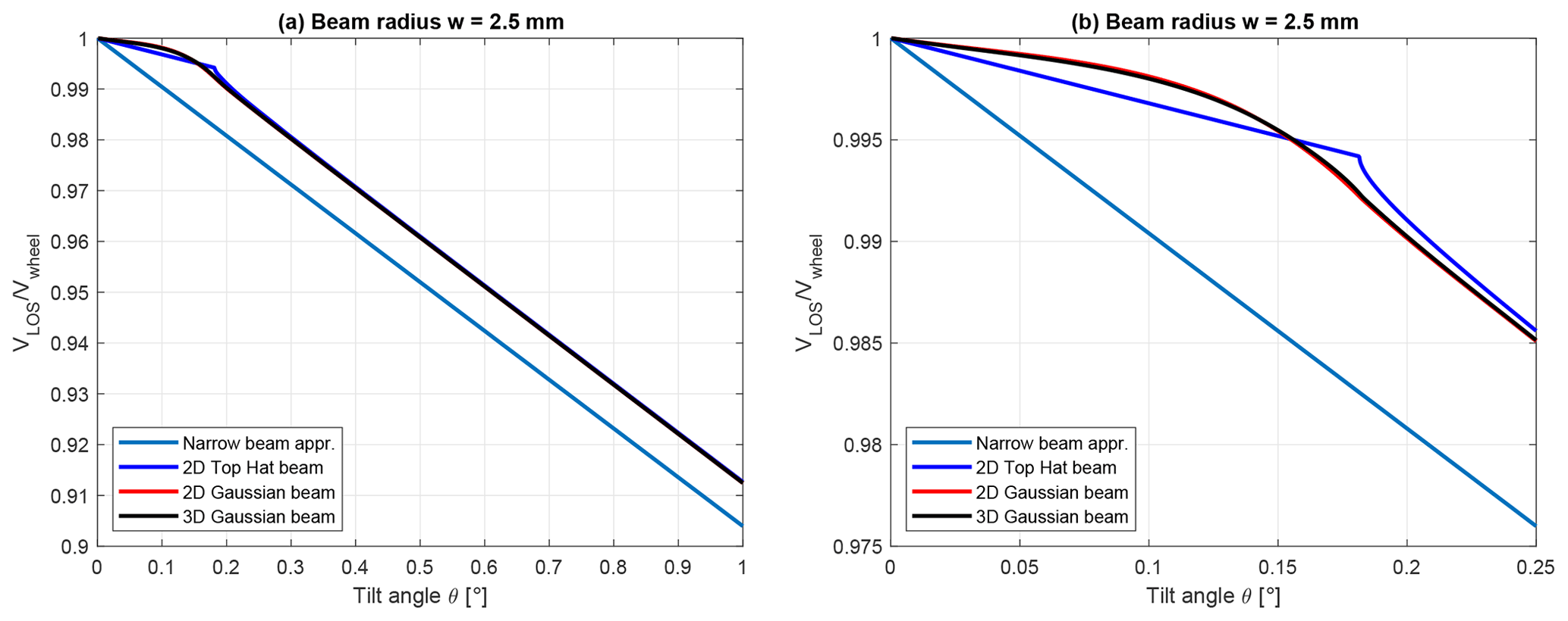
Figure 5Comparison of the different models evaluated for tilt angles from 0 to 1∘ (a) and (b) a close-up focusing on the shallow angles where only a part of the beam touches the wheel. For the chosen beam radius, θ1=0.18∘.
Starting from angles larger than θ1, we see that all the models fall off with the same slope as predicted by the narrow beam approximation. Again, this indicates that as long as the entire beam is on the wheel the sensitivity to a change in tilt angle is the same for all beam widths, and we can use Eq. (6) to calculate this sensitivity. On the other hand, it is also clear that the beam width introduces an offset between the narrow beam and finite width models such that the wider beam measures a slightly higher speed than the narrow. This can be seen as the upper and lower parts of the beam not balancing each other perfectly; because of the curvature of the wheel, the upper part spreads over a wider part of the wheel and therefore a wider range of speeds. This means that the absolute lidar measurement for a given tilt angle depends on the beam width, and it is therefore critical to know this.
For angles smaller than θ1, the models stand out more clearly from each other. The 2-D beam with a top-hat transverse profile drops linearly from θ=0∘ to θ1, where there is an abrupt change followed by a non-linear change in slope, but soon it tends towards the slope of the narrow beam. This abrupt change is due to the discontinuous nature of the assumed beam profile. It should be noted though that due to the abrupt change, the Taylor expansions in Eqs. (6) and (10) actually do not meet in θ1. The two beams with a Gaussian profile behave differently with a smooth transition from the two regimes because near the edges of the beam the laser intensity is lower and therefore contributes less to the individual measurement. It is interesting to see how similar the two Gaussian models behave, indicating that including the third dimension is not critical as long as a Gaussian transverse profile is used.
3.5 Wheel eccentricity
As written in Sect. 2, the wheel, when mounted on the servo motor, has an eccentricity of about 0.01 mm. This eccentricity may come from either the wheel itself or from the mounting on the motor so that the wheel centre and centre of rotation are not perfectly aligned. In order to model the eccentricity and its effect on the calibration, here we will assume the latter, meaning that we model the wheel as being ideal but with its centre offset from the centre of rotation by the amount e. Furthermore, we limit ourselves to regard the beam as having no transverse extent as we did in Sect. 3.1.
Figure 6 shows a schematic drawing of the situation adopting the method of rotating the centre of rotation around the lens. The wheel rotates around the point (xr,yr), and the centre of the wheel, cw, therefore follows a circle of radius e around it. The tangential speed at the intersection between wheel and beam is proportional to the distance, Re, from the rotation centre to the intersection point, and the proportionality constant is of course the angular velocity, ω. Re is a function of the rotation angle ψ. The lidar measures the projection of the tangential speed onto the laser beam and is thus given by VLOS=ω Re (ψ)cos ϕr. From the drawing, we can see that
This means that the dependence on ψ disappears and the measured line-of-sight speed will be the same for all rotation angles. Now, as the wheel rotates, it can happen that the intersection lies to the right of the point xr, as exemplified by the gray-shaded circle, such that ϕr becomes negative, but because the cosine is an even function the measured speed will still be the same. However, it is important to note that the measurement is not unaffected by the eccentricity because the radius of the wheel effectively becomes R+e and is therefore larger than in the non-eccentric case. Also for very small tilt angles there will be a part of the wheel that is not illuminated during a rotation and no measurement will be made. Another thing to notice is that this conclusion will not hold for the thick beam, but as we have seen the narrow beam is really a very good approximation to the general case for angles larger than θ1, which are the angles of interest for the calibration.
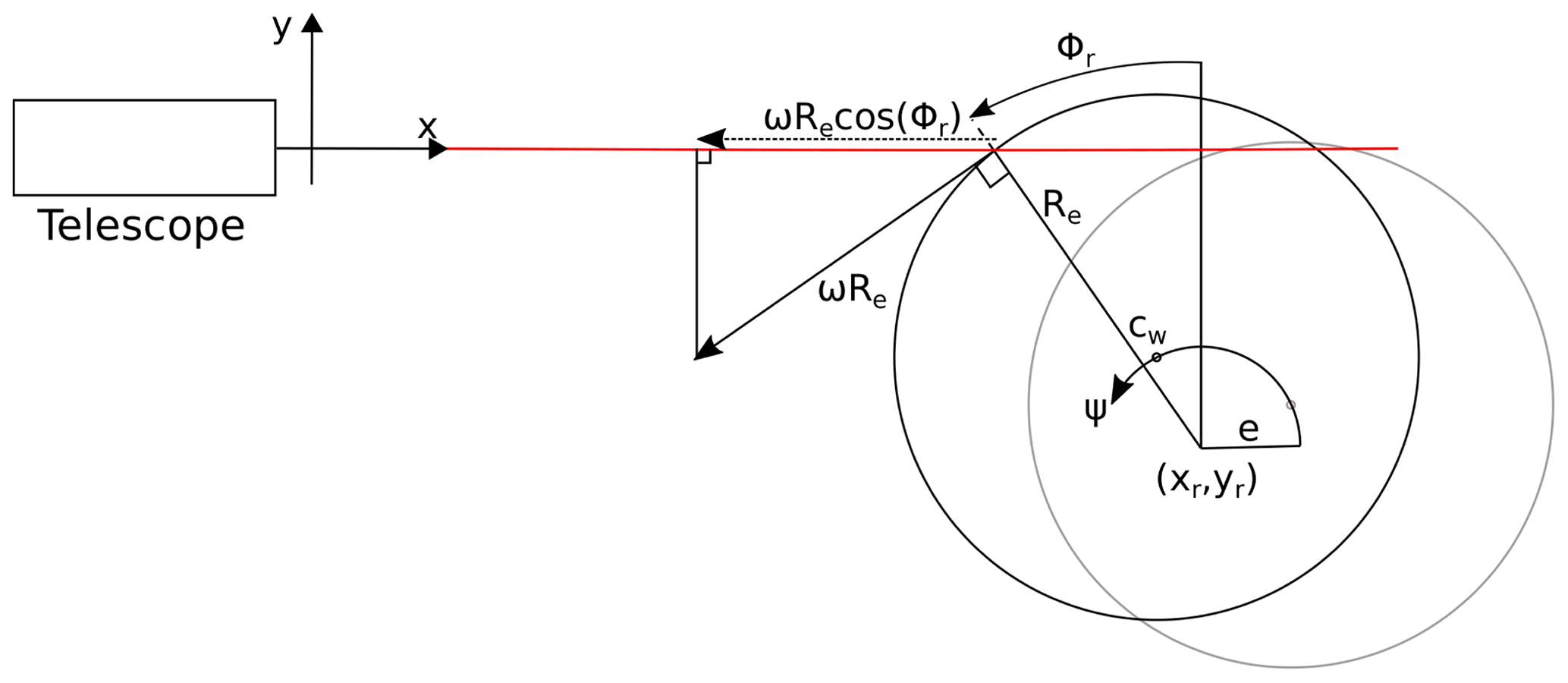
Figure 6Schematic drawing of the influence of the wheel not rotating around its centre point. The wheel rotates around the point (xr,yr) which is offset from the wheel centre, cw, by e.
3.6 Calibration procedure
As we have seen above, our model predicts that there is a linear relationship between the ratio and the tilt angle θ. This means that we can in principle measure the projected speed at any tilt angle larger than θ1 and extrapolate back to the speed at θ0(θ=0), i.e. where the bottom of the beam first touches the wheel, via Eq. (6). However, instead of a single measurement, we choose to measure the projected speed over a range of tilt angles and fit a straight line to the measured values and in that way conduct the extrapolation based on a number of measurements. This is in practice done by slowly turning the tilt adjustment screw on the telescope while synchronously logging Vwheel, VLOS and θ. This method furthermore has the advantage of not relying on a single lidar measurement which can be prone to discretisation uncertainty on the speed estimation. The change in angle causes changes in the LOS speed that span several frequency bin widths, and fitting over this range of angles will tend to average out the errors on the individual measurements.
The difficulty with the method lies in establishing the angles θ0 and θ1, i.e. where the beam just starts to touch the wheel and when the entire beam is on the wheel, as illustrated in Fig. 7a. In our setup, the telescope is not perfectly aligned horizontally with the top of the wheel, and therefore the laser beam is not perfectly horizontal at θ0, as shown in the figure. It is therefore necessary to establish θ0 in a way other than a direct angle measurement with the inclinometer. For extremely shallow tilts, the lidar only occasionally detects a signal, maybe due to the slight eccentricity of the wheel or differences in the surface characteristic, meaning that some parts of the wheel perimeter extend further into the laser beam or reflect stronger than others. We choose the angle of this first sporadic signal as our best estimate for θ0.
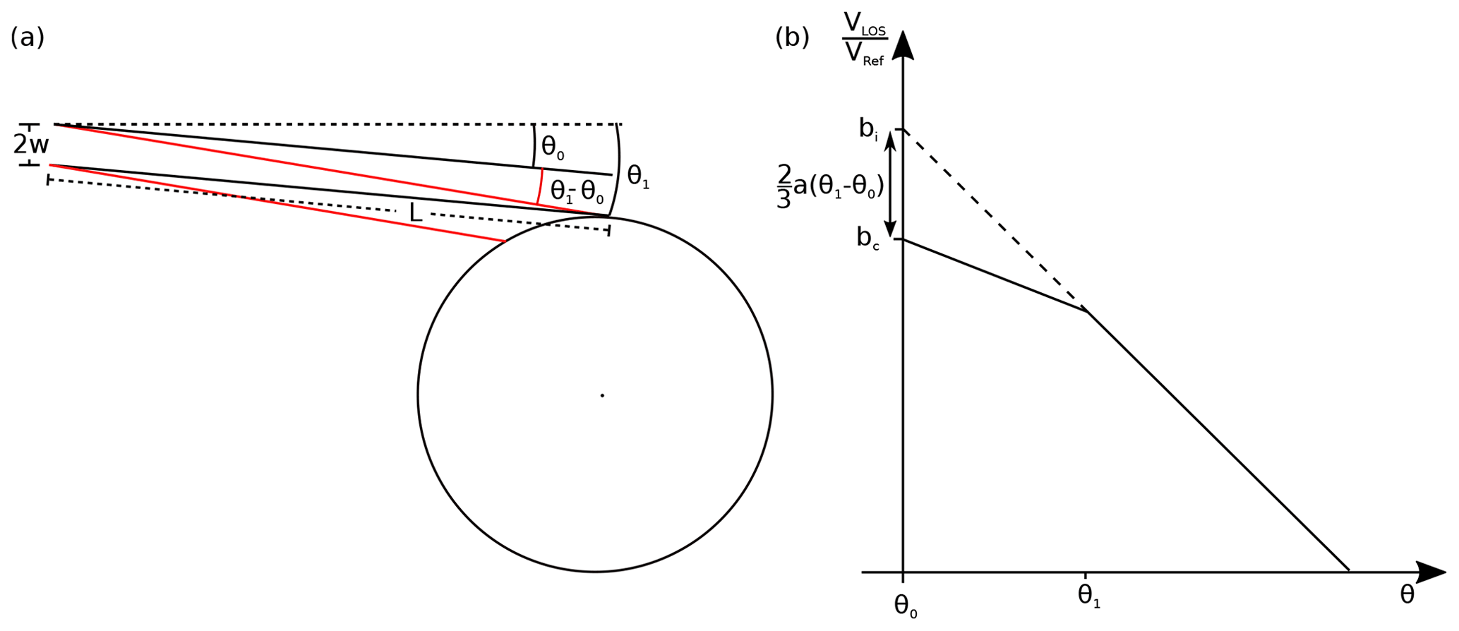
Figure 7(a) Illustration of the definition of θ0 and θ1. θ0 is the angle compared to horizontal where the bottom of the beam first touches the wheel (beam drawn in black) and correspondingly θ1 is the angle where the top of the beam first touches the wheel (red beam). (b) Illustration of the relation between the angles θ0 and θ1, and the fit intercept bi and the corrected intercept bc.
The second angle, θ1, is more difficult to find and is more important for the overall calibration uncertainty. As the beam is slowly lowered from θ0, the gaps between meaningful measurements become shorter and fewer until eventually a continuous lidar signal is achieved. This means that enough of the beam is now touching the wheel for a signal to be detected for all rotation angles, and we choose the angle where this first occurs as the our best estimate for θ1. Effectively, we have thereby also estimated the beam radius as
where .
Another complication to the calibration arises due to the offset introduced by the finite beam width, as explained in Sect. 3.4 and illustrated in Fig. 7b. From the figure, it is obvious that extrapolating from angles larger than θ1 will lead to an overestimation of the speed at θ0, and it is therefore necessary to compensate for this. We will do this via Eqs. (6) and (10), which state that the speed ratio is
where is the slope predicted by the models, but instead we will use the slope of the actual linear regression while assuming that the relationship still holds. From this, the overestimation can be
In the end, we arrive at an estimate of the ratio between speed measured by the lidar and the reference wheel speed given as
where bi is the intercept of the fitted straight line at θ0 and bc is the compensated intercept. As we saw in Sect. 3.4, Eq. (18) is strictly not correct because of the non-linear drop in close to θ1, as shown in Fig. 5, but for small values of w the resulting error is small.
In this section, we will give an estimate of the uncertainties associated with the various parameters going into the calibration and of course the overall calibration uncertainty. First, the uncertainty on the reference speed is estimated, then the uncertainty on the tangential speed measured by the lidar, and finally we combine it into a total calibration uncertainty.
4.1 Uncertainty of reference speed (wheel)
From Eq. (1), we know that the speed of the wheel is given as
and the uncertainty, U, on this can be obtained by applying the GUM model (Joint Committee for Guides in Metrology, 2008) and assuming that the uncertainties on the radius and on the rotational speed are uncorrelated
which, in relative terms, becomes
To get an estimate of the relative uncertainty, we will assume an accuracy of 0.05 mm for the wheel radius and that the rotational frequency measurement is derived from a reference frequency that itself has an accuracy of 10−5 (10 ppm). Inserting this into Eq. (23) gives
The standard uncertainty of the wheel speed is thus of the order of 0.02 %.
The calibration flywheel is made of stainless steel which has a thermal expansion of the order of K (Cverna, 2002). Thus, a change in temperature between the room where the radius was measured and the calibration room of 1 K will lead to a change in the reference speed of the same proportion. The temperature has not been monitored during these measurements but assigning an uncertainty of 3 K will lead to a relative uncertainty of 0.0048 % and therefore not contribute significantly to the overall uncertainty.
4.2 Uncertainty of Vwheel measured by the lidar
With the calibration procedure suggested here, the laser beam is slowly tilted more and more, covering a wide range of projected speeds. Since the response in VLOS to a change in θ is almost linear, it is possible to extrapolate back to the angle θ0 by fitting a straight line to the measured data. However, this indirect way of determining the tangential wheel speed is of course associated with different uncertainty contributions. Firstly, there are the tilt angles: the direct angle measurement but also very importantly the estimation of θ0 and θ1. Secondly, there are uncertainties associated with the fit, where noise in the measured values will lead to uncertainties in the forecasted slope and intercept.
Let us begin by looking at the uncertainty of the non-compensated intercept bi. This is obtained from a linear regression which has an inherent uncertainty depending on the number of points in the regression and the level of noise in the measurements. The standard error of the regression, SE, can be calculated as
where we have introduced the symbol , n is the number of observations, and σ is the standard deviation (Lee and Seber, 2003). SE can be regarded as the standard deviation of the noise in the data and can be used to calculate the standard error of the estimated slope (SEa) and intercept (SEb):
where 〈θ〉 is the average of the measured tilt angles. As can be seen, SEa and SEb depend inversely on the square root of the number of observations. For the actual calibrations in this study, the relative SEa is of the order of or 0.01 % and SEb about a tenth of that which is so small in comparison to other contributions that they can be disregarded. Another contribution to the bi uncertainty is the estimation of θ0. Since the intercept between the extrapolation and the ordinate is taken to be the tangential wheel speed measured by the lidar, it is clear that the position of θ0 and the uncertainty of this is of great importance for the measured speed and its uncertainty. As mentioned in Sect. 3.6, θ0 is defined as the angle where the lidar first starts to pick up sporadic backscatter signals from the wheel surface, but there is still an uncertainty associated with this due to the finite resolution, δθ, of the inclinometer used to measure tilt angles. Assuming that the true θ0 is equally likely anywhere within the resolution range (a rectangular probability distribution), the uncertainty on θ0 can be found as
The squared uncertainty on the intercept due to θ0 is thus
where a is the slope of the extrapolation. The resolution of the tilt measurement is δθ=0.01∘, leading to a standard uncertainty of % when applying a slope of 9.5 % per degree, as is found in the measurements; see Sect. 5.1. This uncertainty is of the same order as that of the wheel speed.
We know that bi leads to an overestimation of the speed measured by the lidar and that we need to compensate for this. From Eq. (20), we know that the calibration value compensated for the beam width is given as
and the uncertainty on this can thus be estimated through
where we have assumed that the uncertainties of the input parameters are uncorrelated. and Ua have both been estimated above, and in the following we will find an estimate for UΔθ.
We will assume that the measurement of θ0 and θ1 are each associated with two uncertainty contributions: UθM and UθD. UθM is related to the absolute measurement of θ0 or θ1 and could, e.g. be due to a gain or offset error, and UθD is a discrimination uncertainty due to the finite resolution of the inclinometer. and are correlated because the angles are measured using the same gauge, whereas and are uncorrelated. We can therefore find the squared uncertainty on as
where r is the correlation coefficient. If assumed that are fully correlated and are uncorrelated, we end up with
where UθD is the same as in Eq. (28).
Now, Δθ is in essence our best estimate of the beam width as expressed through Eq. (17) but the validity of this assumption is associated with some uncertainty. As we shall see in Sect. 5.1, the beam radius estimated with this method does resemble what we would expect from a theoretical calculation of the beam radius, but on the other hand there is no reason to believe it to be a completely correct estimate either. This uncertainty must be incorporated into UΔθ, and we do this by adding the term such that
As mentioned above, is quite large, and in the following we will assume it to be 100 % in relative terms such that . For the smallest beam tested in this study, we have Δθ=0.01∘, and this leads to an uncertainty originating from UΔθ of about 0.069 % out of a total of 0.074 %. UΔθ is thus seen to be the dominant term in .
4.3 Overall calibration uncertainty
We can finally find the overall measurement uncertainty. The lidar estimate of the wheel speed is the compensated calibration constant multiplied by the reference wheel speed:
and the squared uncertainty therefore becomes
and relative to Vwheel it is
This means that and therefore UΔθ are the main contributors to the overall calibration uncertainty.
In this section, calibration measurements made with different beam widths and for different reference speeds will be presented.
5.1 Beam width
It is clear from the uncertainty analysis in Sect. 4 that the beam radius, expressed through Δθ, is of great importance for the overall calibration uncertainty. However, the process of establishing the beam width is not trivial even though our beam is well behaved and can be well approximated by a pure Gaussian beam and the equations describing this; see Appendix C. For Gaussian beams in general, the or width of either the electrical field or irradiance is often used to define the beam radius, but in our case it must be defined as the width from which it is possible to detect a signal. This depends on several parameters such as the detection threshold, scattering properties of the wheel surface and also the angle between beam and wheel surface. The best way we have of quantifying this is therefore to measure the tilt angles where we first detect a signal and where we constantly see a signal, respectively. It is clear that there is no guarantee that these angles represent the beam width, and it is therefore associated with a significant uncertainty, but it is the best estimate we can make with the data at hand.
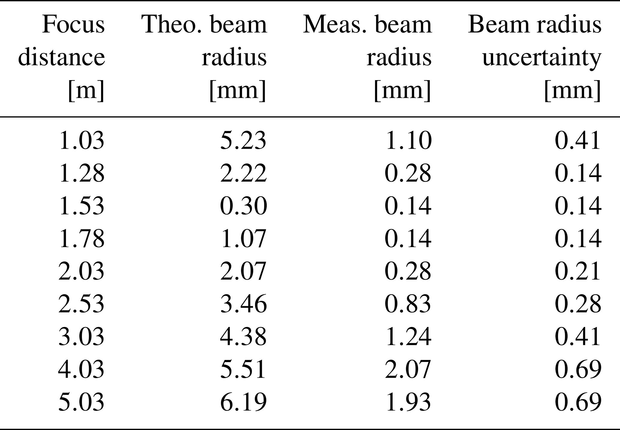
Following the procedure outlined in Sect. 3.6, we have carried out a series of calibrations with different foci of the beam ranging from about 1 to 5 m resulting in different beam widths at the wheel. Figure 8 shows the measured beam radii as a function of focus distance calculated from Eq. (17). Also shown is the theoretical radii of the irradiance calculated using the standard equations for Gaussian beams. The first thing to notice is the clear resemblance in the shape of the two curves, indicating that this is a valid method for estimating the beam width, although the absolute values do not agree. Actually, the values of the calculated widths are about 3 times higher than the measured, but this is not too disturbing since we are not expecting the measured width to represent the width but rather the width from where we can detect a signal. It is more concerning that the minimum around 1.5 m is not nearly as sharply defined for the measured values as for the theoretical, and some of this could possibly be due to the finite resolution of the angle measurement but probably not all of it. The minimum beam radius of 0.14 mm located at 1.53 and 1.78 m actually corresponds to Δθ=0.01∘, which is the same as the angle measurement resolution. Finally, there is the point at 4.03 m which could look like an outlier; the beam width should not be higher with the focus at 4.03 m than at 5.03 m, but this has not been clarified. All in all, it is very difficult do determine the beam radius, and it is thus associated with a large uncertainty. In order to put some numbers on this, we estimate a relative uncertainty of 30 % for the larger beam radii and 50 % and even 100 % for the smallest beams. The resulting absolute uncertainties can be seen in Table 3 together with the theoretical and measured beam widths for each focus distance.
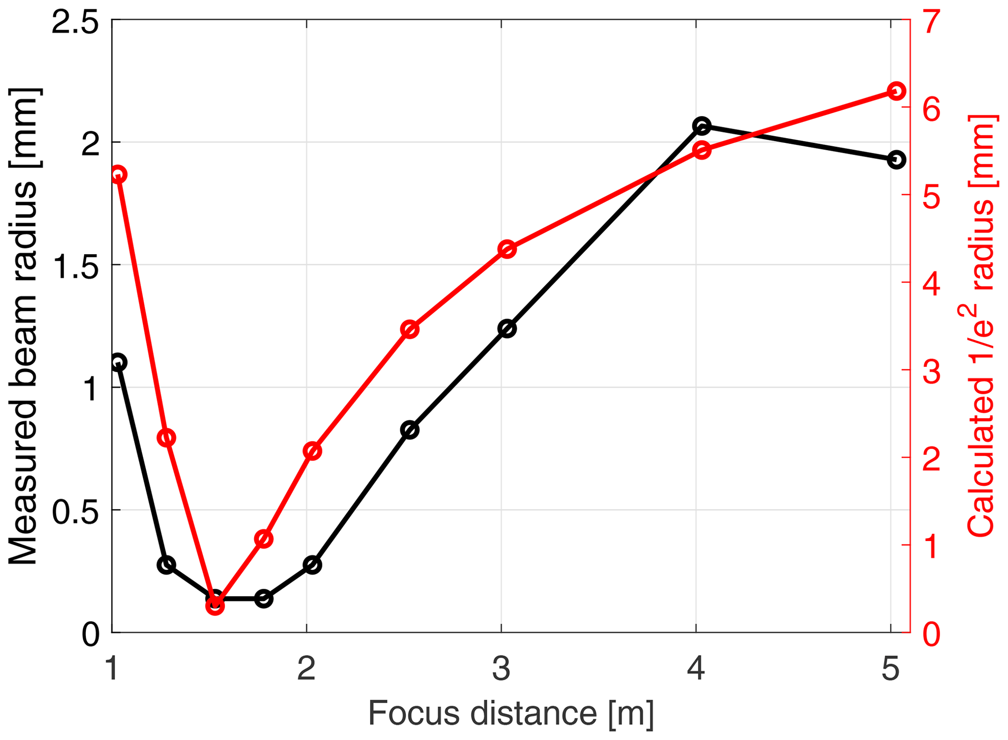
Figure 8Comparison between the measured beam widths and the theoretically calculated radius as a function of focus distance.
Table 3Theoretical and measured beam widths together with estimated uncertainties for the different focus distances used.
Figures 9 and 10 show two examples of the calibrations made. Figure 9 is made with the laser beam focused at 1.53 m and thus with the beam waist located very close to the top of the wheel so that the beam width on the wheel is about as small as the setup allows, while in Fig. 10 the focus is placed at 2.53 m. The mean reference speed is 10.93 m s−1. It is clearly seen how in general falls off linearly as a function of tilt angle as predicted by the models. However, it is also seen that on top of this trend are some discrete steps, something that is also reflected in the residual plot. These steps are due to the narrow beam width resulting in the range of sensed speed being smaller than the resolution of the lidar's Doppler spectrum, causing the speed estimation to jump from bin to bin quite abruptly. In contrast, this feature is almost completely gone in Fig. 10, where the beam is much bigger, and therefore a larger range of radial velocities is covered in each measurement, which spreads the Doppler signal over several bins. This binning effect has an impact on the fit result through the standard error on the slope and intercept, which is indeed higher for the narrow beam, but as mentioned in Sect. 4.2 this effect is still much smaller than other uncertainty contributions. This smoothing effect of the regression can also be seen in the residual plots (lower panel) which have average values of essentially 0 (ranges between and for Figs. 9 and 10, respectively), meaning the fit is very close to the average. The red line in the top panel of the figures is the least-squares fit of a straight line to the measurement data over the range of tilt angles indicated by the extent of the red line itself. The fit ranges over angles from θ0+0.1∘ to 0.1∘ before the maximum measured tilt angle. The resulting fit parameters, slope and intercept, are shown in the insets.
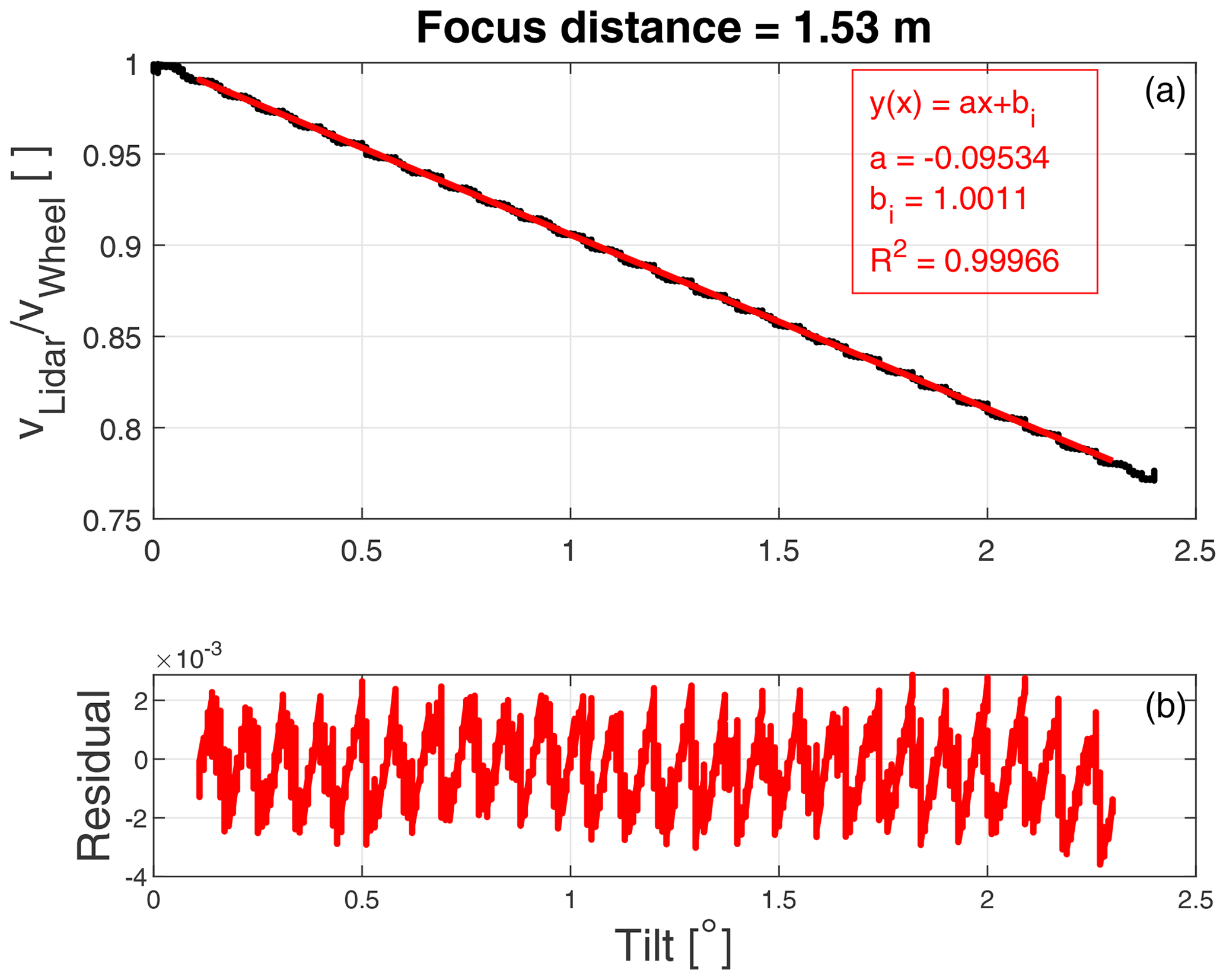
Figure 9Example of calibration measurement made with a focus setting of 1.53 m, meaning that the waist of the beam is placed very close to the top of the wheel. The black curve indicates the measurement data and the red curve indicates a least-squares fit of a straight line to the data. Panel (b) shows the residuals of the fit.
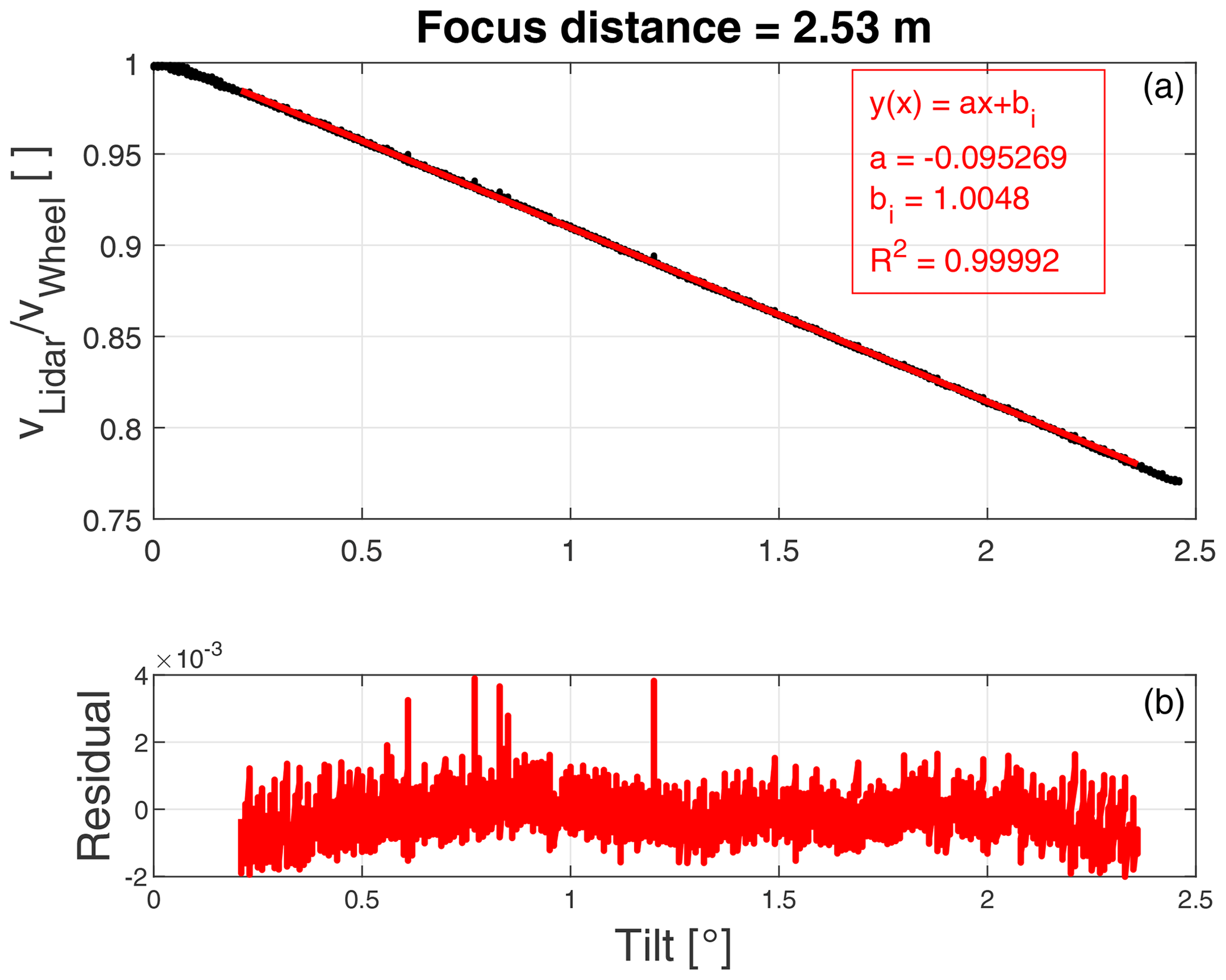
Figure 10Example of calibration measurement made with a focus setting of 2.53 m. The black curve indicates the measurement data and the red curve indicates a least-squares fit of a straight line to the data. Panel (b) shows the residuals of the fit.
Figure 11 shows the fit slopes and intercepts for all nine calibrations as a function of focus distance. According to the narrow beam model, the slope of is which with the parameters specified in Table 1 is equal to −9.60 % per degree. From the figures, it is seen that the measured slopes range from −9.496 % to −9.537 % per degree. This is not a large difference but it is still larger than the estimated uncertainty, and it is more or less the same for all calibrations and not just one or two outliers. The reason behind this deviation is not known.
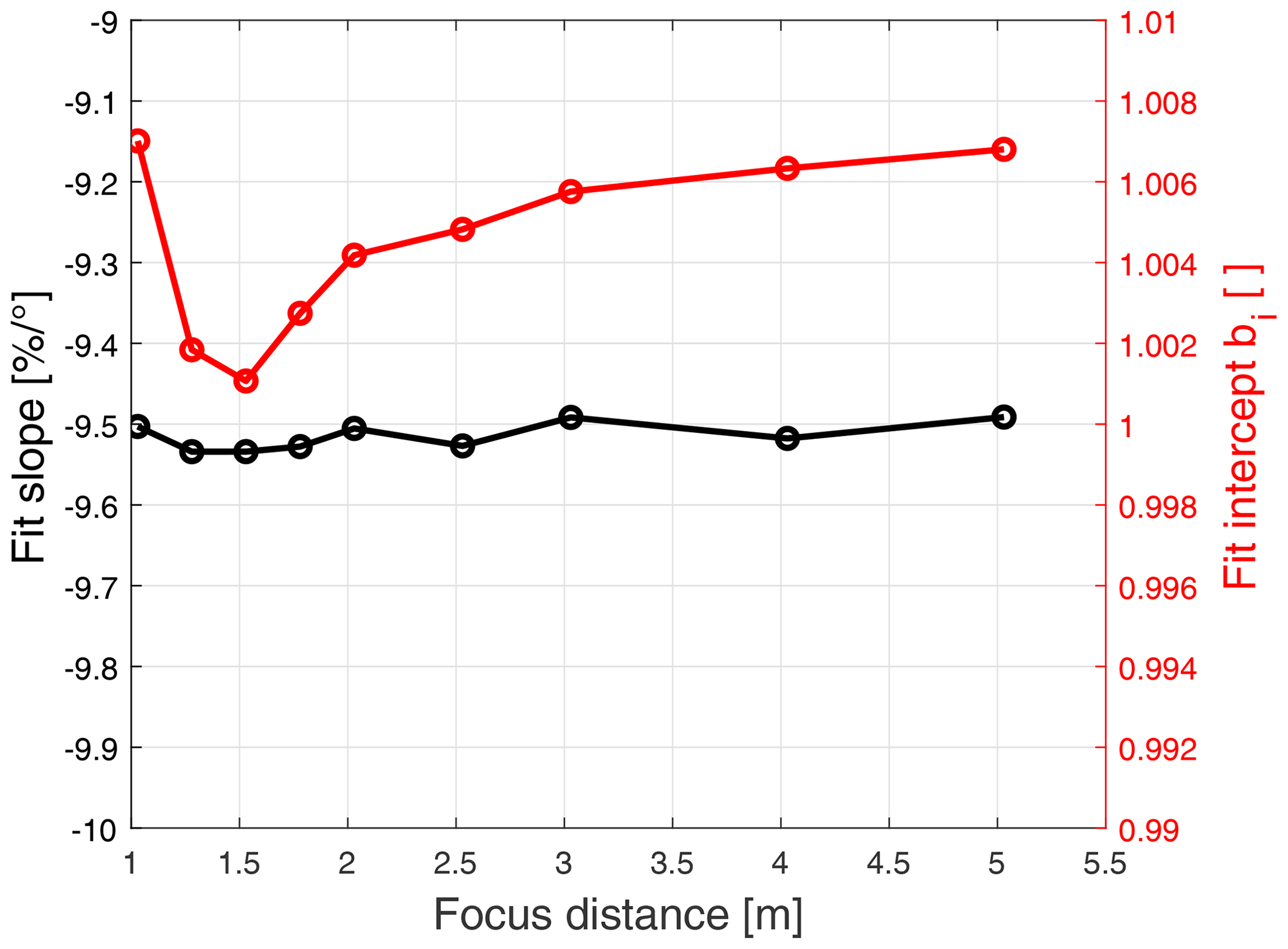
Figure 11Fit slope and intercept as a function of focus distance. The intercept values show a clear minimum at 1.53 m, where the beam width at the wheel is smallest, clearly illustrating the need for compensating these results.
More interesting for the calibration purpose is of course the fit intercept, which is shown in red in Fig. 11. It is clearly seen that the intercept overestimates as expected and in shape the curve looks a lot like the measured beam width in Fig. 8. This highlights the need to compensate the calibration result for this. This has been done in Fig. 12, where the red curve shows the compensated intercept values and the black curves represent the estimated standard uncertainties. The compensation has clearly brought the intercept closer to 1 with the maximum and minimum placed approximately 0.3 % on either side. Most of the points are within or very close to the estimated standard uncertainty, with the exception of the points at 1.78 and 2.03 m. This is probably due to the measurement of Δθ, which seems low compared to the theoretical value as seen in Fig. 8, and therefore the compensation becomes too weak. The combined uncertainties calculated using the equations derived in Sect. 4 range from about 0.08 % for the narrow beams up to about 0.9 % for the widest beams, and it is clearly seen how the shape of the uncertainty curve follows that of the measured beam width in Fig. 8. This is due to the term , which we have estimated to be equal to the value of Δθ and which is dominating. This underlines the importance of a good estimate of the beam width.
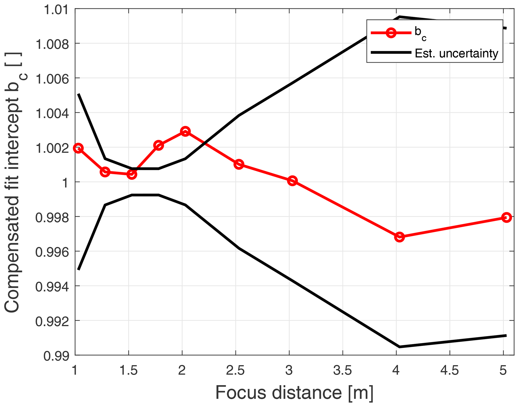
Figure 12Compensated regression intercepts together with the estimated standard uncertainties.
5.2 Different reference speeds
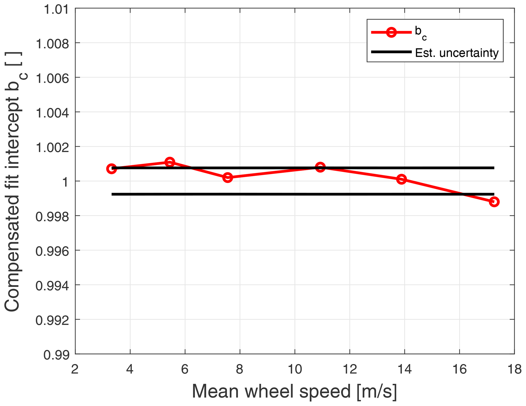
In this section, we present the results of calibrations made with different reference speeds but a fixed focus distance of 1.53 m, i.e. with the smallest possible beam width at the wheel.
The tested reference speeds range from about 3.3 to 17.3 m s−1, and Figs. 13 and 14 show two examples of measurements and fits made at 5.44 and 13.89 m s−1, respectively. In both cases, there is very good agreement with what is expected from the model as well as with the results in Sect. 5.1. It is noted that the characteristic staircase shape also seen in Fig. 9 is very pronounced in both of these figures, but that the length of each “step” seems to change with the reference wheel speed. This is because what is plotted is the ratio between measured and reference speeds, and for low reference speeds the bins of the Doppler spectra become relatively larger as a function of tilt angle.

Figure 13Example of calibration measurement made with a reference speed of 5.44 m s−1 and a focus distance of 1.53 m. The black curve indicates the measurement data and the red curve indicates a least-squares fit of a straight line to the data. Panel (b) shows the residuals of the fit showing some distinct oscillations because of the speed estimation jumping from bin to bin due to the very narrow beam.
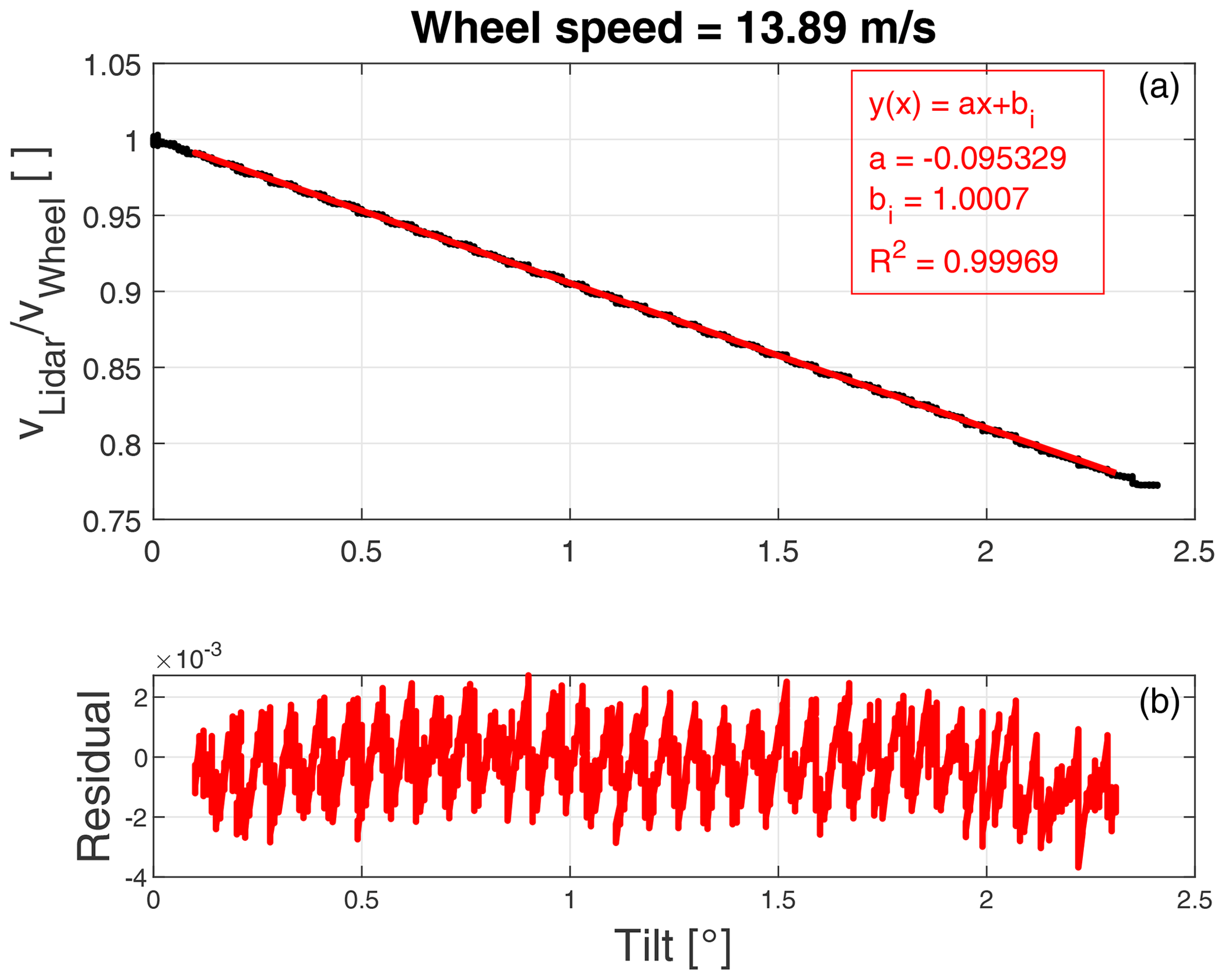
Figure 14Example of calibration measurement made with a reference speed of 13.89 m s−1 and a focus distance of 1.53 m.
Figure 15 shows the resulting fit parameters for all the tested reference speeds. We see that the slope of the fit lies between −9.51 % and −9.56 % per degree and is more or less constant across the tested speeds. Also the fit intercept is very close to constant for the first five tested speeds and is bounded within 0.998 and 1.002, and thus within the estimated uncertainty, but the last point at 17.26 m s−1 stands out a bit. Here, the intercept drops to below 1 but is still within the uncertainty. A possible explanation for this is that at 17 m s−1 the wheel rotates at around 9.5 revolutions per second, which is quite fast, and the entire rig including transceiver and inclinometer starts to shake, which limits both lidar and angle measurements.
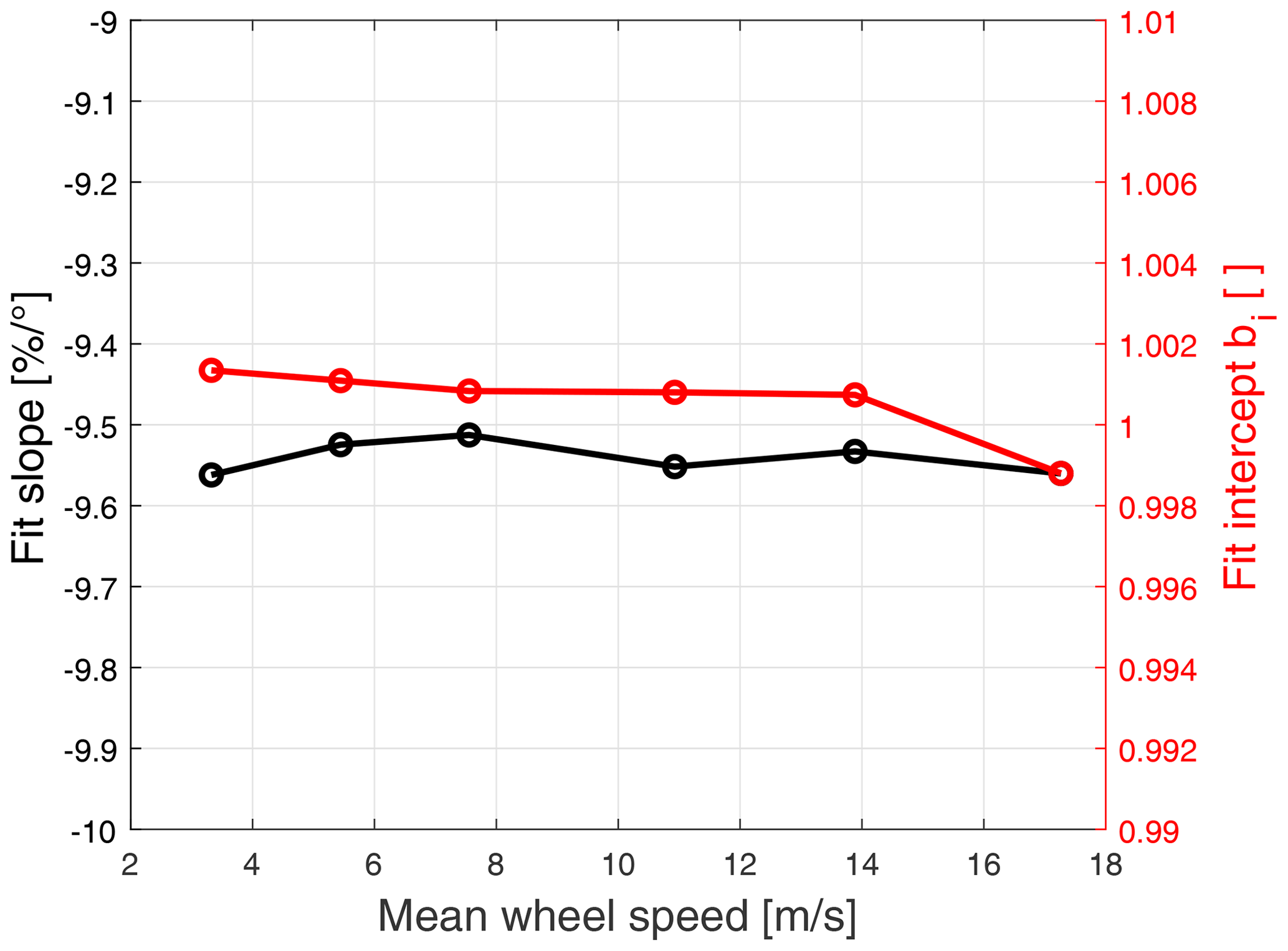
Figure 15Results of fits for different reference speeds. Fit intercept is not compensated for w.
Again, the regression intercepts have been compensated and the result is shown in Fig. 16 together with the uncertainties. Because of the small beam width used in these measurements, the difference between bi and bc is very small. The assumed uncertainty on Δθ is the same as for the same focus distance in the previous section and the resulting combined standard uncertainty is about 0.08 % which most of the points lie close to.
It can seem paradoxical to use a flywheel to calibrate a Doppler wind lidar when the parameter we want to measure, the peripheral speed, is the one thing the lidar cannot measure. Nevertheless, the presented measurements and analysis show that the proposed calibration method is not only practically feasible but could actually lead to a significant reduction in calibration uncertainty compared to the current practice. However, there could also be other methods for achieving a similar calibration result. For instance, it seems more straightforward to measure a linear motion along the direction of the beam. This might very well be the case because besides directly measuring the desired parameter, the uncertainties introduced by the angle measurement and assessing the zero point of the angle scale together with the beam width can be alleviated. On the other hand, there are also arguments for using the flywheel, as discussed earlier, by scanning a range of speeds and fitting, the inherent uncertainty due to discretisation is reduced. The symmetrical nature of the wheel makes it easy to obtain a very stable reference speed, whereas with a linear motion the target would probably have to be moved back and forth and thus accelerated up to a known speed repeatedly. This would then require the position of the reference target to be logged together with its speed, which again demands a more complicated geometrical model. Another idea could be to measure in a range of angles covering the direction toward the centre of the wheel. In this way, a zero point defined as the angle where the beam is perpendicular to the wheel surface could be established as a place where no speed is measured, thus alleviating the problems seen above with finding θ0 and possibly θ1. In this case, the calibration uncertainty would depend critically on the angle measurement uncertainty. Unfortunately, the calibration setup does not allow for such a measurement to be made due to limitations in the attainable tilt angles.
The uncertainty analysis shows that the main uncertainty contributor is UΔθ, which essentially depends on the beam width estimation. An estimate for Δθ based on the tilt angles for the first sporadic and the first stable measurements, respectively, was proposed. Another approach that could potentially reduce this uncertainty is to measure the backscatter level as a function of tilt angle. In this way, the backscatter signal would increase strongly from θ0 to θ1 as the overlap between beam and wheel increases and then remain more or less constant when the entire beam is on the wheel. Unfortunately, our lidar in its present state does not measure or store the backscatter level, and therefore this approach has not been tested.
Inspired by a similar concept commonly used for calibrating LDAs, we have constructed a setup for calibrating coherent Doppler wind lidars based on a spinning flywheel with the lidar beam skimming the wheel's periphery. The setup is made in such a way that the laser beam can be tilted and thus probe different projections of the wheel's tangential speed. A simple model shows that there is a linear relation between the beam tilt angle and the measured LOS speed. This can be utilised to extrapolate back to the true tangential speed at zero tilt, which is the one angle otherwise impossible to measure at because the physical overlap between wheel surface and laser beam disappears. The model takes into account the finite width of the laser beam but only under the assumption that the beam is collimated, while in reality the beam used in the tests is actually focused in order to control the beam radius. The model also forms the basis of the uncertainty analysis which concludes that a total calibration standard uncertainty of about 0.1 % can be achieved with this setup, which is approximately an order of magnitude better than current practice. The uncertainty analysis reveals that the main contributor to the total uncertainty is the finite radius of the laser beam, and in order to reduce the uncertainty it is essential to determine this better than we have been able to achieve so far. Calibration measurements performed at different reference speeds and with different beam widths all show good agreement with the model and confirm that the lowest calibration uncertainty is achieved when the beam width is minimised.
In this section, we discuss how the ratio as a function of tilt angle for a beam of small but finite width is approximately the same as that for an infinitely narrow beam.
If we apply Taylor's expansion to the third order to Eq. (8), we get
and if we further make the approximations,
where is the mean of and , and δ is a small perturbation, we get
which is seen to be equal to Eq. (6).
The result of Eq. (15) can be reached in the following way:
The theoretical beam width at the top of the wheel can calculated by an appropriate combination of the following two equations: the width of an untruncated Gaussian beam at a distance x′ from the beam waist can be calculated through
where w0 is the width at the waist and λ is the laser wavelength (Siegman, 1986). Similarly, w0 can, with the waist placed a distance x from the focusing lens, be found as
where wl is the beam width at the lens.
The measurements and scripts for data analysis can be found at https://doi.org/10.11583/DTU.11991189 (Pedersen, 2020).
ATP was responsible for measurements, data processing, data analysis, model development and manuscript writing. MC was responsible for the conceptual idea, model development and manuscript writing.
The authors declare that they have no conflict of interest.
Torben Mikkelsen and Steen Andreasen are gratefully acknowledged for initiating, designing and constructing the calibration rig. All members of the DTU Wind Energy, TEM, measurement systems engineering team are thanked for their great help and support. The anonymous reviewers are gratefully thanked for thorough and constructive criticism.
This research has been supported by the Danish EUDP (grant no. project TrueWind (64015-0635)).
This paper was edited by Gerd Baumgarten and reviewed by three anonymous referees.
AMO GmbH: Incremental angle measuring systems based on the AMOSIN – Inductive Measuring Principle, available at: http://www.amoitalia.it/pdf/Catalogo%20rotativi_WMI_EN_2013_08_21.pdf (last access: 21 February 2020), 2013. a
Angelou, N., Foroughi Abari, F., Mann, J., Mikkelsen, T., and Sjöholm, M.: Challenges in noise removal from Doppler spectra acquired by a continuous-wave lidar, in: Proceedings of the 26th International Laser Radar Conference, 26th International Laser Radar Conference ILRC26, Porto Heli, Greece, 25–29 June 2012, S5P-01, 2012. a
Bean, V. and Hall, J.: New primary standards for air speed measurement at NIST, Metrology – at the Threshold of the Century Are We Ready?, Proceedings of the 1999 NCSL Conference, Charlotte, NC, USA, 11–15 July 1999, 413–421, 1999. a
Courtney, M.: Calibrating nacelle lidars, available at: https://orbit.dtu.dk/files/57802786/Calibrating_nacelle_lidars.pdf (last access: 27 January 2021), DTU Wind Energy E, 0020, 2013. a
Cverna, F.: ASM ready reference – Thermal properties of metals, ASM International, Materials Park, Ohio 44073-0002, USA, ISBN 978-0-87170-768-0, 2002. a
Duncan, M. L. and Keck, J.: Considerations for Calibrating a Laser Doppler Anemometer, in: Proceedings of Measurement Science Conference (MSC), Anaheim Marriott, Garden Grove, California, USA, 2009. a
Joint Committee for Guides in Metrology: Evaluation of measurement data – Guide to the expression of uncertainty in measurement, available at: https://www.bipm.org/utils/common/documents/jcgm/JCGM_100_2008_E.pdf (last access: 22 January 2021), 2008. a
Joint Committee for Guides in Metrology: International vocabulary of metrology – Basic and general concepts and associated terms (VIM), available at: https://www.bipm.org/utils/common/documents/jcgm/JCGM_200_2012.pdf (last access: 22 January 2021), 2012. a
Lee, A. J. and Seber, G. A. F.: Linear regression analysis, Wiley, ISBN 978-0-4714-1540-4, https://doi.org/10.1002/9780471722199, 2003. a
Pearson, G. N., Roberts, P. J., Eacock, J. R., and Harris, M.: Analysis of the performance of a coherent pulsed fiber lidar for aerosol backscatter applications, Appl. Optics, 41, 6442–6450, 2002. a
Pedersen, A., Foroughi Abari, F., Mann, J., and Mikkelsen, T.: Theoretical and experimental signal-to-noise ratio assessment in new direction sensing continuous-wave Doppler lidar, J. Phys. Conf. Ser., 524, 524–532, https://doi.org/10.1088/1742-6596/524/1/012004, 2014. a
Pedersen, A. T.: Flywheel calibration of coherent Doppler wind lidar – data, https://doi.org/10.11583/DTU.11991189, 2020. a
Shinder, I. I., Crowley, C. J., Filla, B. J., Moldover, M. R., Stop, M., and Drive, B.: Presented at the 16th International Flow Measurement Conference, Flomeko 2013 Improvements To NIST's Air Speed Calibration Service realizing the primary standard, in: International Flow Measurement Conference, Paris, France, 24–26 September 2013, 1–9 pp., 2013. a, b
Siegman, A. E.: Lasers, University Science Books, available at: https://app.knovel.com/hotlink/toc/id:kpL000001E/lasers/lasers (last access: 22 January 2021), ISBN 978-0-935702-11-8, 1986. a
Wagenaar, J., Bedon, G., Werkhoven, E., and van Diggelen, C.: Wind Iris nacelle LiDAR calibration at ECN test site, available at: http://resolver.tudelft.nl/uuid:940be7e6-04d8-475a-bd84-23799c2da736 (last access: 27 January 2021), ECN-X-16-116, 2016. a
- Abstract
- Introduction
- Calibration rig and lidar
- Model and calibration procedure
- Uncertainties
- Calibration measurements
- Discussion
- Conclusions
- Appendix A: Approximation to the 1-D model
- Appendix B: 3-D beam
- Appendix C: Width of Gaussian beam
- Code and data availability
- Author contributions
- Competing interests
- Acknowledgements
- Financial support
- Review statement
- References