the Creative Commons Attribution 4.0 License.
the Creative Commons Attribution 4.0 License.
 | 08 Mar 2022
Low-level buoyancy as a tool to understand boundary layer transitions
Francesca M. Lappin
Tyler M. Bell
Elizabeth A. Pillar-Little
Phillip B. Chilson
Advancements in remotely piloted aircraft systems (RPASs) introduced a new way to observe the atmospheric boundary layer (ABL). Adequate sampling of the lower atmosphere is key to improving numerical weather models and understanding fine-scale processes. The ABL's sensitivity to changes in surface fluxes leads to rapid changes in thermodynamic variables. This study proposes using low-level buoyancy to characterize ABL transitions. Previously, buoyancy has been used as a bulk parameter to quantify stability. Higher-resolution data from RPASs highlight buoyancy fluctuations. RPAS profiles from two field campaigns are used to assess the evolution of buoyancy under convective and stable boundary layers. Data from these campaigns included challenging events to forecast accurately, such as convection initiation and a low-level jet. Throughout the daily ABL transition, results show that the ABL height determined by the minimum in vertical buoyancy gradient agrees well with proven ABL height metrics, such as potential temperature gradient maxima. Moreover, in the cases presented, low-level buoyancy rapidly increases prior to the convection initiation and rapidly decreases prior to the onset of a low-level jet. Low-level buoyancy is a force that is sensitive in space and time and, with further analysis, could be used as a forecasting tool. This study expounds on the utility of buoyancy in the ABL and offers potential uses for future research.
- Article
(9592 KB) - Full-text XML
- BibTeX
- EndNote


The atmospheric boundary layer (ABL) is strongly influenced by kinematic and thermodynamic interactions with the Earth’s surface. It is sensitive to changes in radiation, low-level moisture, and heat fluxes. The ABL functions as a conduit for moisture and momentum to be transported vertically. As a consequence, the depth of the ABL (referred to herein as ABL height) and the ABL stability fluctuate in time and space (Lenschow et al., 1979; Stull, 1988). This influences local weather (Lapworth, 2006), turbulence (Banta et al., 2003; Bonin et al., 2013), and aerosol transport (Nilsson et al., 2001; De Wekker et al., 2009; Pal et al., 2014). The nature of the ABL makes it crucial to successful numerical weather prediction (NWP) yet incredibly difficult to represent. Most boundary layer parameterizations are based on observation methods that are decades old. Often, the best choice for boundary layer parameterizations is situationally dependent to what is being modeled (Braun and Tao, 2000; Nolan et al., 2009; Hu et al., 2010; Cuchiara et al., 2014; Cohen et al., 2015). Weather and climate models will continue to struggle to accurately represent the ABL without vertical, high-resolution observations (Steeneveld et al., 2008; Teixeira et al., 2008; Baklanov et al., 2011). Assimilating in situ data has been shown to benefit the performance of the model (Ruggiero et al., 1996; Otkin et al., 2011; Jonassen et al., 2012; Ágústsson et al., 2014; Reen et al., 2014; Jones et al., 2016; Degelia et al., 2018). The lack of accessible technology to accurately sample the ABL has slowed advancements throughout the field. Up until recently, these types of data have not been easily retrievable.
In the past, it has proven difficult to collect adequate spatially and temporally resolved measurements within the ABL, resulting in a data gap. Since the National Research Council (2009) called for more vertical measurements in the ABL, there have been technological advancements to address the gap. Remote sensors such as microwave radiometers, lidars, and scatterometers can continuously measure the lower atmosphere, which have been shown to improve short-term forecasts (Coniglio et al., 2019; Hu et al., 2019; Lewis et al., 2020). However, these instruments are expensive and typically need to be used in tandem to obtain a complete sample. Most remote sensors are mobile but not nimble, which limits the environments they can sample. For example, pre-convection environments change rapidly, and instruments need to relocate quickly to gain targeted observations. Another tool more commonly used to capture ABL measurements is radiosondes, which are typically released twice daily across the United States. Their upper-air measurements aid greatly in seeing synoptic patterns throughout the troposphere. Unfortunately, radiosondes are only released frequently enough to capture mesoscale changes during field experiments. The spatial and temporal frequency of radiosonde release is inadequate for convection allowing models. Of equal importance is that their spatial resolution through the ABL is too coarse for a thorough characterization. While there are avenues to shrink the data gap, we still lack an infrastructure to address this on a broader scale.
Increasing interest in remotely piloted aircraft systems (RPASs) across many sectors has accelerated improvements in quality and availability of RPAS technology (Reuder et al., 2009; Elston et al., 2015; Villa et al., 2016). In turn, the capabilities of RPASs have broadened and its usefulness in research became obvious. The benefits of utilizing RPASs in atmospheric sciences have been proven across many situations, including turbulence observations and data assimilation (Dias et al., 2012; Båserud et al., 2016; Flagg et al., 2018; Barbieri et al., 2019). RPASs can be readily reused to sample rapidly changing environments and can be paired with remote sensors to describe the lower troposphere more completely. In Bell et al. (2020), measurements from RPASs, radiosondes, and remote sensors were found to agree well with each other. The study also discusses the functionality of each platform. While RPASs allow for more adaptive sampling, there are more federal regulations and air restrictions governing their use. Nonetheless, some specially designed RPASs can deliver equally accurate measurements, as radiosondes with a higher spatial resolution and are more cost-efficient. The confidence shown in the data collection and usefulness in data assimilation will prove its place as a reliable observation platform. RPASs stand as an affordable, portable option that can be used in tandem with remote sensing platforms for a more complete sampling of the ABL.
Diurnal cycles in temperature and humidity characterize ABL transitions, driving changes in ABL height and stability. However, other processes can have additional effects on how the ABL transitions to different states. For example, advection and subsidence are difficult to quantify but play important roles in transitions (Angevine et al., 2020). Additionally, clouds can have varying effects on ABL transition periods (Brown et al., 2002), all of which can also affect the ABL height. There are numerous ways to determine the ABL height, many of which are described and tested in Dai et al. (2014) and Dang et al. (2019). Notably, potential temperature proved to be a highly accurate method of estimating ABL height with vertical data resolution of less than 20 m (Dai et al., 2014). Similarly, sharp gradients in humidity have been used to determine the ABL height for both stable and convective boundary layers when using lidar data (Hennemuth and Lammert, 2006). Dang et al. (2019) also evaluated different systems to determine the ABL height, which did not include RPASs, and determined that lidar-based profiles would benefit NWP. A common thread throughout these studies is that there is neither a perfect determination for ABL height, nor is there a perfect platform (Seibert et al., 2000; Dai et al., 2014; Dang et al., 2019). While there will always be benefits and drawbacks to observation platforms, it is possible that RPASs could marry some of the pros, while reducing costs. Alongside the evolution of sampling strategies, there are new ways to determine the ABL height.
Buoyancy is a fundamental force in fluids caused by density differences that can drive vertical acceleration. Buoyant parcels rise from the warm surface and convectively mix the ABL. This process is the foundation behind most gradient-based ABL height methods previously mentioned. Angevine et al. (2020) uses a surface buoyancy flux framework to define stages in ABL transition periods. Additionally, it has been used in attempts to forecast severe weather. Buoyancy is the basis for convective parameters like convective available potential energy (CAPE) and convective inhibition (CIN). CAPE is the buoyancy integrated between the level of free convection and the equilibrium level, which may not always exist in every environment. In contrast, CIN is the culmination of negative buoyancy which suppresses the thermal lift. Since CAPE is a bulk parameter, the most substantial influence comes at the middle troposphere. Climatologically, CAPE has correlated directly with storm intensity (Zhang and Klein, 2010) but has little short-term prognostic value (Ziegler and Rasmussen, 1998). CAPE and CIN lack the small-scale, near-surface effects needed to understand convection initiation (CI). As a result, mean radiosonde-derived values of CAPE and CIN do not significantly differ between deep convection and fair weather days (Zhang and Klein, 2010). Yet, in the same study, the average low-level (< 5 km) buoyancy does significantly differ. Moreover, single-level simulated buoyancy values rapidly intensify, overcoming entrainment dilution prior to CI (Houston and Niyogi, 2007; Trier et al., 2014). Additionally, buoyancy is used to quantify cold pool strength. Simulations indicate that an ample cold pool is the key to long-lasting quasi-linear convective systems (Weisman and Rotunno, 2004). Another facet of buoyancy is its influence on modeled low-level jet (LLJ) speed. The strength of positive buoyancy had a direct relation with the maximum wind speed for southerly LLJs (Shapiro and Fedorovich, 2009; Shapiro et al., 2016). Conversely, large positive buoyancy impedes the initiation of northerly LLJs, such that negative buoyancy is beneficial to the northerly LLJs (Gebauer et al., 2017). Proper understanding of LLJs has implications on deep convection, air quality, and wind energy.
In short, the utilities of buoyancy have been shown by models, yet few studies have substantiated the results with in situ observations. Recent developments in RPASs allow us to gather the necessary measurements to test these hypotheses in real environments. Alongside the evolution of observation platforms, there is an opportunity to advance the methods. The time–height evolution of buoyancy under different ABL phenomena will be analyzed. Using the high spatiotemporal resolution data from rotary-wing RPASs, ABL features and transitions will be dissected. The following analysis will include two cases, namely the diurnal ABL cycle under the influences of an LLJ and pre-convection conditions at two locations within an elevated valley. The goal is to expound on the unique advantages gained by viewing ABL processes through the lens of buoyancy.
Here we consider examples of data collected using RPASs and radiosondes during two different field campaigns. Both campaigns aimed to display the usefulness of RPASs under various atmospheric phenomena. The Flux Capacitor campaign sampled boundary layer transitions under a common Southern Plains occurrence, the LLJ. The Lower Atmospheric Process Studies at Elevation – a Remotely Piloted Aircraft Team Experiment (LAPSE-RATE) campaign was uniquely located at high altitude with orographically driven circulations and different land surfaces. An aerial map of each location can be found in Fig. 2 of Bell et al. (2020). We will use these data to evaluate the utility of low-level buoyancy in various environments. All flights completed during both campaigns were conducted under Federal Aviation Administration (FAA) certificates of authorization (COA) and overseen by FAA licensed pilots, who were integrated with the research teams. A complete description for each campaign follows.
2.1 Flux Capacitor
The Flux Capacitor field campaign took place as a test of the 3D Mesonet concept in which a subset of Oklahoma Mesonet stations would include an RPAS capable of regularly profiling the lower troposphere (Chilson et al., 2019). The campaign tested the feasibility of continuous flights to observe the ABL transition over a 24 h period. Flights began at 15:01 UTC (10:01 LST) on 5 October 2018, taking off every 30 min, and with the last flight at 14:30 UTC (09:30 LST) on 6 October 2018. A flight to 1 km above ground level (a.g.l.) takes roughly 12 min. This campaign sampled the ABL throughout its diurnal cycle and under southerly LLJ conditions. The flight ceiling for Flux Capacitor was based on line-of-sight operations up to 1200 m. Flights took place 28 km southwest of Norman, OK, USA, at the Kessler Atmospheric and Ecological Field Station (KAEFS), which is co-located with the Oklahoma Mesonet's Washington station (WASH). Additionally, a radiosonde was released approximately every 3 h, for a total of 10 soundings. Radiosondes served as a way to validate measurements from RPAS profiles.
2.2 LAPSE-RATE
LAPSE-RATE took place in San Luis Valley, Colorado, USA, from 14–19 July 2018 (de Boer et al., 2020a). In total, 10 teams gathered to collect atmospheric measurements using RPASs for three targeted missions, i.e., CI, drainage flows, and boundary layer transition. Teams distributed across the valley regularly collected synchronized, vertical profiles of the atmospheric state up to 914 m a.g.l. with rotary-wing RPASs. Additional data were collected using fixed-wing RPASs, radiosondes, and ground-based remote sensors. Although there were many other RPASs and remote sensing platforms used, we will focus on the Center for Autonomous Sensing and Sampling (CASS) deployed stations. This allows for direct comparisons with the Flux Capacitor campaign, as the same RPAS was used. CASS had three profiling stations. The two main sites were at Moffat School (MOFF) and Saguache Municipal Airport (K04V), approximately 27 km northwest of MOFF. To capture the cold-air drainage, the team relocated from K04V to Saguache Farms (SAGF) on 19 July 2018, but these data will not be included. The base flight frequency was 30 min, but during an ABL transition, such as pre-convection or drainage flow reversal, the frequency was increased to every 15 min.
This campaign was unique in location and execution. The San Luis Valley has an average elevation of 2300 m and peaks at 4000 m above sea level. The valley is arid but contains irrigated cropland creating gradients in temperature and moisture from differing land uses. There is orographic lift, which leads to convection commonly occurring overtop the mountains. Furthermore, mountain–valley circulations affect ABL transitions and air quality. Teams were able to partially sample the valley, which is nearly the size of Connecticut, by completing over 1200 flights, using 34 different platforms (de Boer et al., 2020b; Pillar-Little et al., 2021). Conditions within the valley were ideal for RPAS flights and observing mesoscale to microscale flow features. de Boer et al. (2020b) provided a description of the weather conditions. In summary, due to limited moisture, temperature and humidity have a strong diurnal cycle that drives flow features. In the afternoon, when the ABL is approximately dry adiabatic, winds are gustier and occasionally enhanced by outflow from mountain convection. The first 2 d of the structured flights (15–16 July 2018) were selected to study CI. Both days had moisture advected from the Pacific Ocean with a passing cold front. The 19th of July was focused on capturing cold-air drainage flow; hence, flights began shortly before sunrise.
During the LAPSE-RATE campaign, there were numerous RPASs collecting data in addition to remote sensing platforms and ground station observers. All data obtained during LAPSE-RATE can be found at https://zenodo.org/communities/lapse-rate/ (last access: June 2021). Flux Capacitor utilized the CopterSonde RPASs, radiosondes, and surface observations. In order to have direct comparisons between the two datasets, we chose to only use the data from radiosondes and the CopterSonde. The description of these two platforms follows.
3.1 CopterSonde
The RPAS utilized in both field campaigns was the CopterSonde 2. This is a rotary-wing quadcopter designed and manufactured by CASS at the University of Oklahoma. The CopterSonde contains three temperature sensors (iMet-XF glass bead thermistors) and three relative humidity sensors (Innovative Sensor Technology, IST AG, HYT 271). These are placed within the shell of the aircraft, protecting them from solar radiation and heat from the motor, which can impact the precision of the measurements (Greene et al., 2018, 2019). Pressure is determined by the MS5611 pressure sensor which is built into the autopilot board to aid in altitude control. Built into the shell is an aspirated intake scoop that is designed to consistently draw air across the sensors. It features a sampling technique that adapts to position the intake scoop into the wind. An algorithm using roll, pitch, and yaw details from the autopilot determines the wind speed and direction. Consequently, this improves the measurement accuracy and eliminates the need for additional wind speed and direction sensors (Segales et al., 2020; Greene et al., 2019). The sensor scoop was tested in the Oklahoma Climatological Survey Calibration Laboratory. The bias for each sensor is calculated and applied to the CopterSonde data, which is further described in Segales et al. (2020). These adjustments build on trials from previous campaigns such as the Environmental Profiling and Initiation of Convection (EPIC; Koch et al., 2018) and 2018 Innovative Strategies for Observations in the Arctic Atmospheric Boundary Layer (ISOBAR; Kral et al., 2021).
CopterSonde and radiosonde data gathered in these campaigns were compared in Bell et al. (2020), in addition to data from the Collaborative Lower Atmospheric Mobile Profiling System (CLAMPS; Wagner et al., 2019). Temperature, humidity, and wind speed and direction from each system were compared and showed strong agreement.
3.2 Radiosonde
Radiosondes have stood as the standard for atmospheric measurements for over 90 years and have served as a validation tool for many novel sensing platforms. The Vaisala RS92-SGP radiosonde was used for this study. Data from the radiosondes are initiated from ground station data. According to Vaisala technical data, there is a 0.5 ∘C uncertainty for temperature and 5 % uncertainty for relative humidity. The measurement response time for both sensors is less than 0.5 s. Data are recorded and transmitted at 1 Hz. Further information regarding the radiosondes used during LAPSE-RATE can be found in Bell et al. (2021).
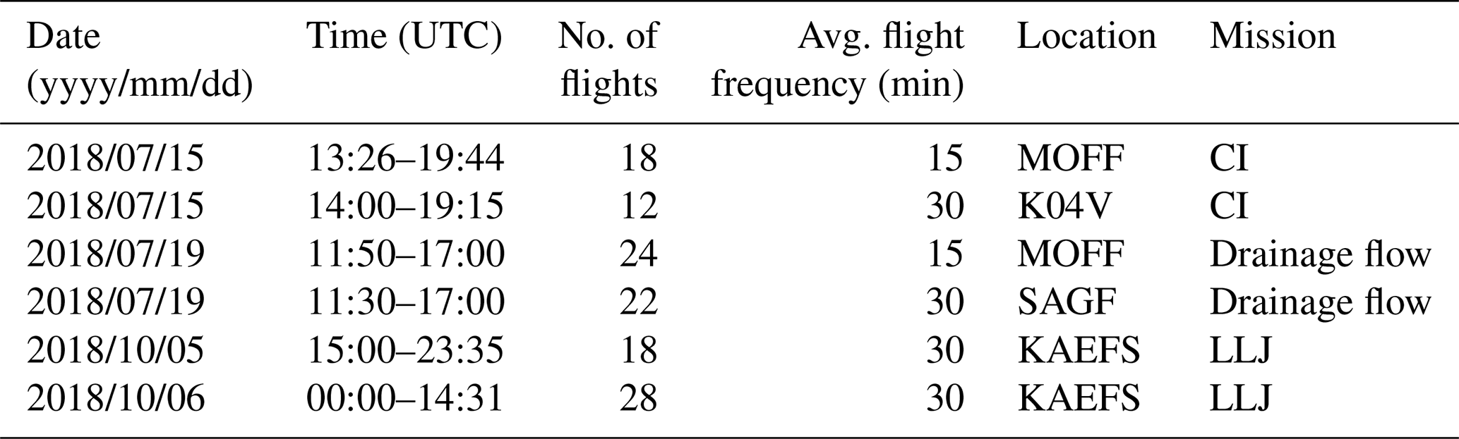
The CopterSonde allowed for controlled measurements taken at a prescribed frequency specified by the needs of each campaign. Table 1 describes the flight strategies in both experiments. Abiding by FAA air regulations, the flight ceiling for Flux Capacitor was 1524 m (5000 ft) a.g.l., with line-of-sight operations required. Lights affixed to the RPASs allowed visibility into the night, but due to high winds, a majority of Flux Capacitor flights did not reach the flight ceiling. As for LAPSE-RATE, flights were authorized up to 914 m (3000 ft) a.g.l., which most flights reached.
Table 1Summary of CopterSonde flights from Flux Capacitor and LAPSE-RATE.
Buoyancy (β) was calculated at each level, using Eq. (1), such that the vertical resolution is the same as all other variables. The parcel's virtual temperature (Tv,par) was calculated based on parcel theory, with the lowest observed temperature and dew point used as the initial inputs. The temperature and relative humidity measured by the RPASs or radiosondes are used to calculate the virtual temperature which functions as the environmental temperature (Tv,env), while g is the acceleration due to gravity.
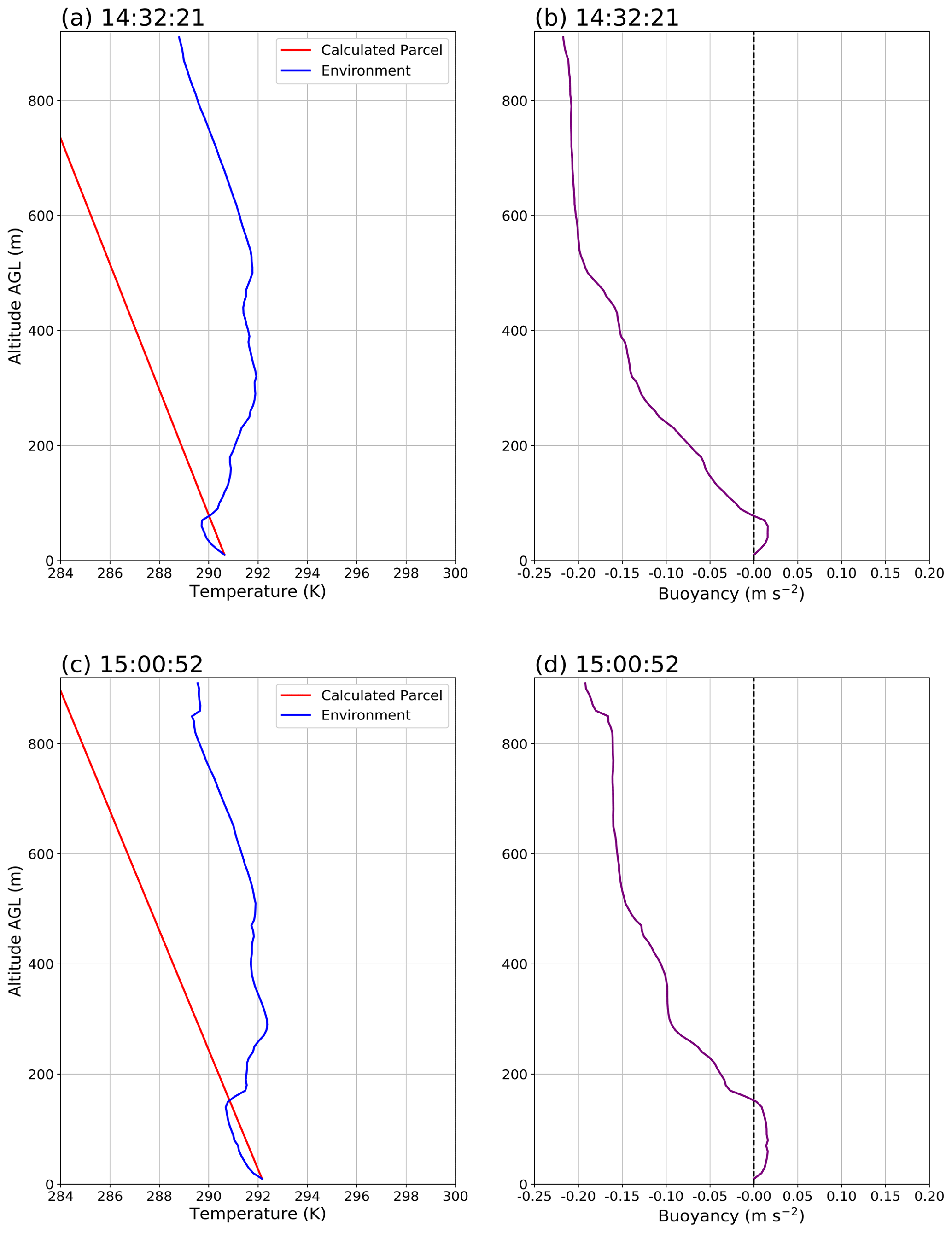
Figure 1Temperature (K) and buoyancy (m s−2) profiles from CopterSonde at MOFF on 19 July 2018. (a, c) Temperature observed from CopterSonde (blue) and the dry adiabatically lifted parcel (red). (b, d) Buoyancy profile (purple) shown with the black dashed line at neutral (zero) buoyancy. All times are in UTC.
CopterSonde data were recorded at 10 Hz and then downsampled to a 3 m vertical resolution for Flux Capacitor and 10 m for LAPSE-RATE. As for the radiosondes, the data were vertically interpolated to mimic the sampling resolution of the CopterSonde. Example profiles Tv,par, Tv,env, and β, using CopterSonde data, are provided in Fig. 1. The detailed account of how the LAPSE-RATE data were processed can be found in Pillar-Little et al. (2021). The summed buoyancy for the radiosondes was calculated up to the flight ceiling for the CopterSonde closest to the release time. Since flight ceilings change based on flying conditions, this was done to make the results most comparable.
To determine the ABL height during Flux Capacitor, two methods are used. The control method finds the height of the maximum vertical potential temperature gradient, hereafter called potential temperature method. It was chosen because it has shown to be applicable in stable and convective boundary layers over land (Martucci et al., 2007). The hypothesized method finds the height of the minimum buoyancy gradient, hereafter called buoyancy method. Above a convective boundary layer, there is a capping inversion, and the atmosphere becomes more stable; above a stable boundary layer, there is a residual layer which is less stable. Therefore, the height of the ABL should be found where the buoyancy begins to sharply decrease in magnitude. In Fig. 1, this would be approximately where the buoyancy profile intercepts the zero buoyancy line, since the slope is very small. To smooth over some individual spikes in the CopterSonde data, a five-point (15 m) running mean is applied across the entire profile to derive quantities including, potential temperature, dew point temperature, mixing ratio, and buoyancy. Since these values are not directly observed, the calculations to attain these values may have introduced noise. This is not necessary for the radiosonde data since it was processed by Vaisala software and then additionally vertically interpolated.
5.1 Case 1: Flux Capacitor
Radiosondes and the CopterSonde were regularly deployed, allowing them to be cross-evaluated. Both platforms share similarities in the quantities and dimension sampled. Nonetheless, there are stark differences in their abilities. Radiosondes are capable of sampling a much higher column, while the CopterSonde's flight ceiling is limited greatly by the regulation, technology, and atmospheric conditions. Radiosondes are not true Eulerian profilers; they are advected with the flow, adding quasi-Lagrangian impacts. As a result, observations are coming from downwind of the release site, especially for the Flux Capacitor since there was a strong LLJ. The CopterSonde conducts fixed location profiles, delivering true local vertical gradients. Moreover, the cost of a radiosonde profile is much higher than a CopterSonde profile, thus restricting the temporal resolution of radiosonde releases. Nevertheless, the long-established confidence in radiosondes makes them a validation tool for measurements from the CopterSonde. Figure 2 shows the temperature at the lowest measured elevation from both platforms, in addition to the Oklahoma Mesonet’s 9 m temperature observation. Given the thermistor response time of < 2 s, the CopterSonde has enough time to acclimate to the air temperature at 6 m. The radiosondes used in this field campaign take in the station measurements as a boundary condition, which explains the strong agreement between radiosondes and Mesonet data. Initially, the CopterSonde has, approximately, a 1 ∘C warm bias at the lowest elevation. This is a consequence of the shell being heated by the Sun during the setup of the site. Continuous aspiration over the sensors above the surface would reduce this effect at higher elevations. The recurrent flights that followed prevented the CopterSonde from sitting in the direct sunlight long enough to heat up; thus, the warm bias reduces below 0.5 ∘C after 16:07 UTC. Keeping the instrument in the shade until takeoff is now the standard to mitigate this effect. Therefore, there is confidence in the accuracy of temperature measurements and, thus, the initialization point for buoyancy profiles.

Figure 2Time series of temperature (∘C) measured at the lowest level from the Mesonet (9 m; blue line), CopterSonde (6 m; black dot), and radiosondes (7 m; red dot) on 5–6 October 2018. Purple and orange vertical lines represent sunset and sunrise, respectively.
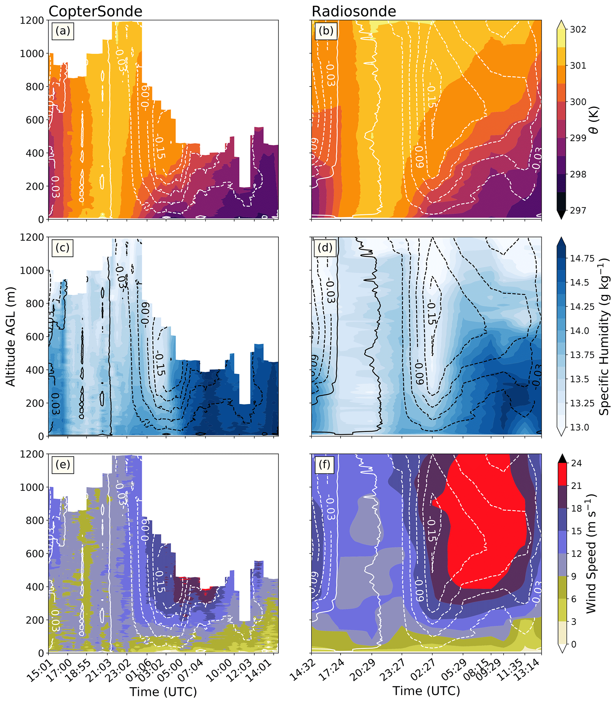
Figure 3Shaded contour fields on 5–6 October 2018 of (a, b) potential temperature (K), (c, d) specific humidity (g kg−1), and (e, f) wind speed (m s−1), with the buoyancy contours overlain (m s−2) at KAEFS. Dashed (solid) contours are negative (positive). Panels (a), (c), and (e) use CopterSonde data, and panels (b), (d), (f) use radiosonde data.
Figure 3 shows the contours of calculated buoyancy in time and height from the CopterSonde (left) and the radiosondes (right) over environmental variables. Profiles from each platform are interpolated over time and height to create the continuous figures. While the vertical interpolation is the same, the radiosonde data are interpolated over 3 h compared to the CopterSonde's 30 min period. Assuming that the environment changes linearly over 3 h is likely inaccurate, especially during ABL transitions such as morning or evening. As a result, the ABL morning transition (14:32–17:24 UTC) looks much smoother with the radiosonde data (Fig. 3b, d). The atmosphere’s turbulent nature is highlighted by fine-scale changes in the wind speed shown by the increased vertical data resolution with the CopterSonde coupled with the increased frequency of profiles (more flights). The change in flight ceilings seen in Fig. 3e shows the limitations of flying in a high wind environment. Nonetheless, the change in buoyancy throughout the time period is similar for both platforms. After 21:03 UTC, the surface cools rapidly as the insolation decreases, and a shallow inversion initiates a stable boundary layer. The buoyancy’s rate of change is of interest, from 01:30–04:30 UTC, when a negative gradient forms before the onset of the LLJ. The negative buoyancy is at its peak in an elevated layer when the LLJ forms there about 1 h later. The buoyancy gradient aligns with a declining moisture gradient (Fig. 3c, d). This could be attributable to the downwelling of drier, warmer air before the LLJ. Figure 2 shows a local maximum in temperature at the time of the maximum wind speed (from 400–1200 m). As the warmer air aloft is mixed down, there is a slight rise in the buoyancy at around 05:30 UTC (Fig. 3a, b). The shear instability acts to enhance turbulent mixing and degrade the stable layer to approach a neutral state. Without it, the negative buoyancy would suppress the turbulence and lead to greater stratification. The LLJ disrupts the potential temperature gradient by redistributing cooler air vertically. Figure 3a shows that the surface cooling beneath the jet is not as strong due to mixing. Additionally, there is moisture advected beneath the southerly jet. If the stratification remained, fog may have formed. While the temperature field indicates the formation of a stable boundary layer, buoyancy provides more information about the timing and layer which the jet forms. In short, buoyancy helps to delineate the interconnections between the LLJ and the ABL.
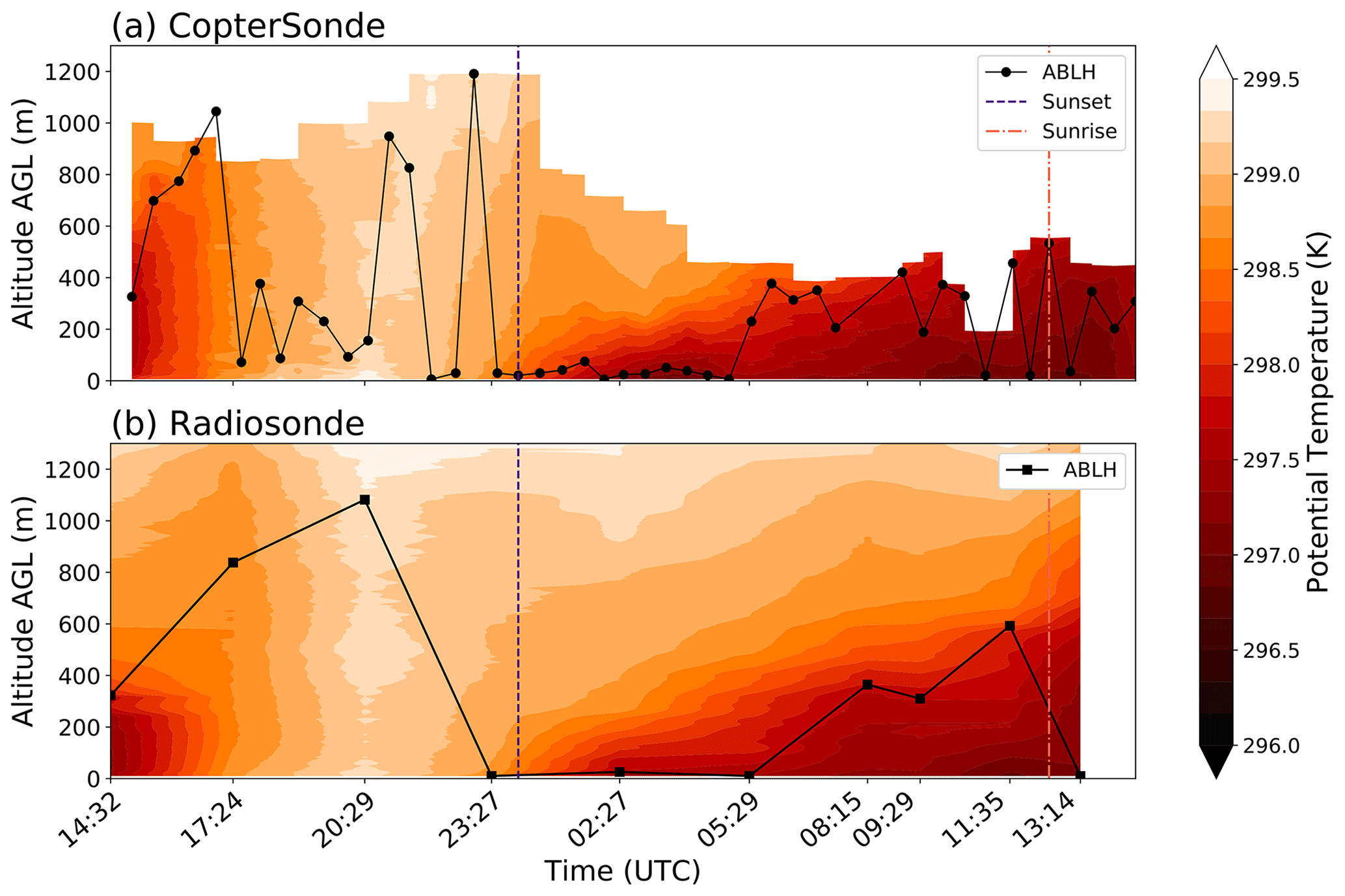
Figure 4Potential temperature field (shaded contours) and black line indicating the ABL height determined by the height of the maximum potential temperature gradient on 5–6 October 2018 at KAEFS. (a) Each circle indicates the height determined by an individual flight. (b) Each square indicates the height determined by an individual radiosonde.
After the initial analysis seen in Fig. 3, it was observed that buoyancy is roughly constant with height in a convective boundary layer. This is expected since buoyancy is a driving force to homogenize the ABL. Therefore, we propose a gradient-based method to find the ABL height from buoyancy profiles. In order to evaluate a new method, the ABL heights determined from the potential temperature method are also found (Martucci et al., 2007). The potential temperature method and radiosonde-derived heights (Fig. 4b) do not change as rapidly as those derived from the CopterSonde data (Fig. 4a). Moreover, the potential temperature method ABL heights from the CopterSonde data are lower from 17:24–23:00 UTC, compared to radiosonde-derived heights. It is worth noting that some heights appear to surpass the provided data; this is a smoothing artifact from plotting. The drop-off in ABL height occurs once the mixed layer extends past the flight ceiling. Without a strong transition above the ABL, the potential temperature method erroneously finds where the surface layer transitions to the mixed layer. The CopterSonde is more likely to find these sharp gradients near the surface because of the increased data resolution at lower levels. Considering that most ABL height methods are tested using radiosonde data, it is expected that the potential temperature method works well.
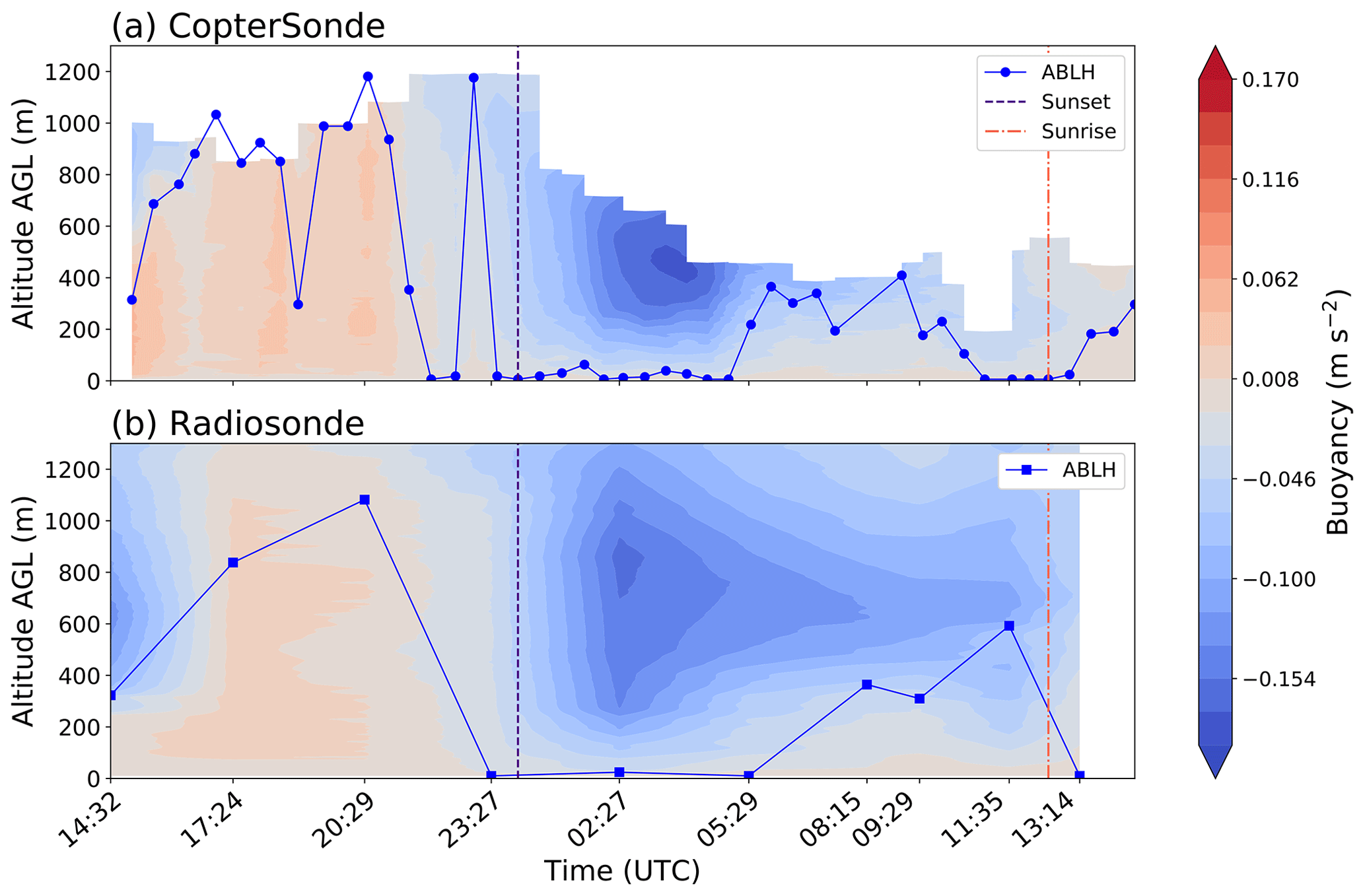
Figure 5Same as Fig. 4 but with buoyancy field and buoyancy-determined ABL heights (blue line).
It is worth pointing out the differences in sampled potential temperature. Around 14:32–15:00 UTC, the height of the mixed layer disagrees strongly between the two sampling platforms (Fig. 4). The depth of the mixed layer determined by a radiosonde release is around 330 m (Fig. 4b), while it is around 550 m for the CopterSonde (Fig. 4a). Although, the ABL heights are the same between both platforms. A measurement bias is not suspected; it is likely due to the radiosonde being advected downwind. Figure 3f shows 15–18 m s−1 winds in the 350–970 m layer, directly above the ABL top (Fig. 5). Between the 14:30 UTC radiosonde release and the first CopterSonde flight at 15:01 UTC, the radiosonde would likely be many kilometers downstream of KAEFS. The difference in mixing layer depths can also be seen in the buoyancy data (Figs. 3, 5). The shallow positive buoyancy region found by the radiosonde leads to a much more negative vertically summed buoyancy value compared to the nearest CopterSonde observation (Fig. 6).
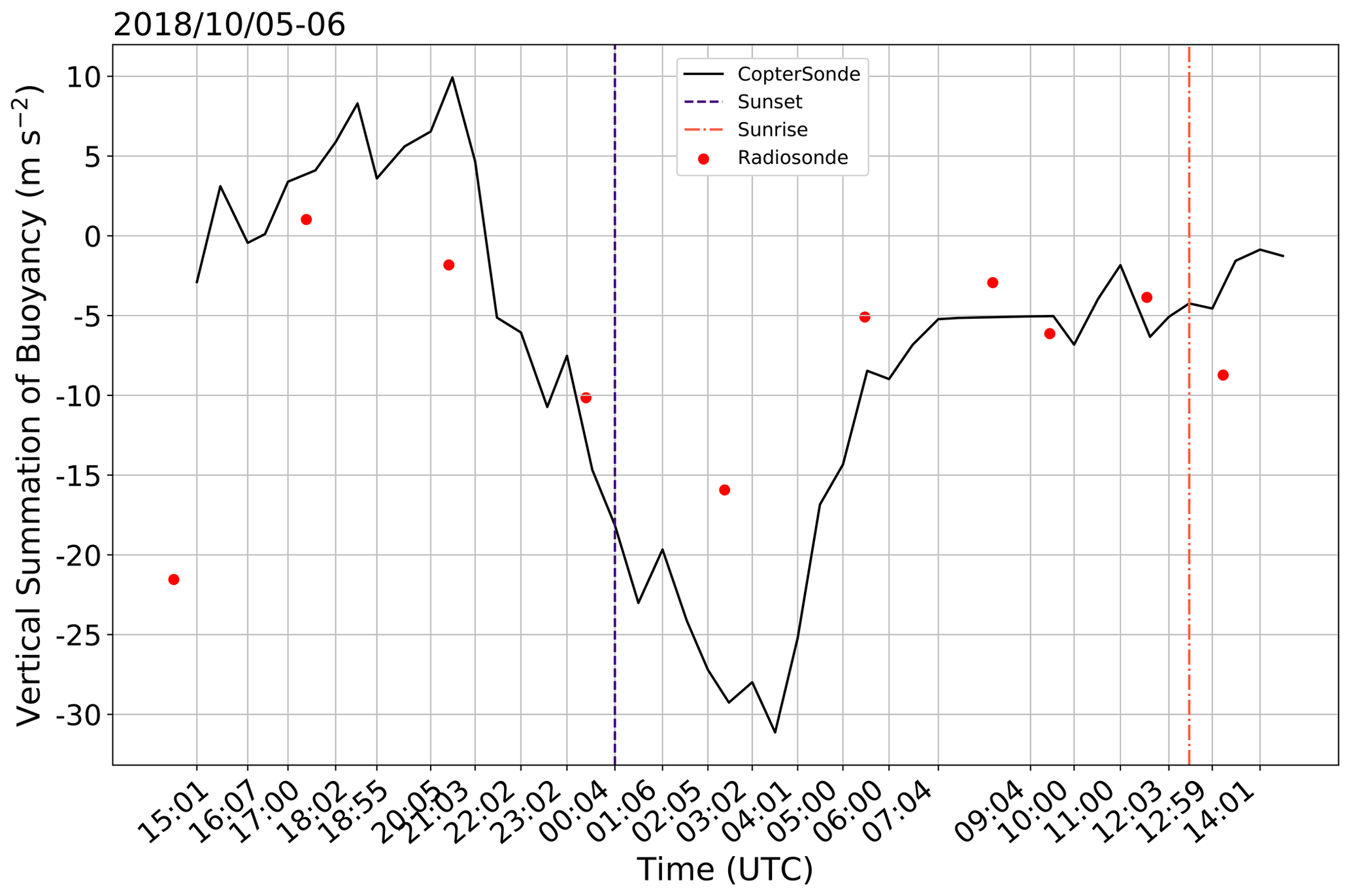
Figure 6Time series of vertically summed buoyancy (m s−2) on 5–6 October 2018. The black line is the CopterSonde data, and red dots are the radiosonde data. Purple and orange vertical lines represent sunset and sunrise, respectively.
The proposed buoyancy method is applied to both datasets, as seen in Fig. 5. Unlike the CopterSonde-derived heights using the potential temperature method (Fig. 5a), the buoyancy method provides more consistent, realistic heights. The 17:24–23:00 UTC time period has more agreement from profile to profile (Fig. 5a) and with the radiosonde-derived heights (Fig. 5b). Furthermore, the radiosonde-derived heights using the potential temperature method (Fig. 4b) and buoyancy method (Fig. 5b) are identical throughout the entire period. The correlation (r=1.0) between the buoyancy method and potential temperature method bolsters our confidence that the buoyancy method is promising to determine ABL heights. Once the jet arrives and mechanically mixes the surface layer, there is a rise in ABL heights across all methods and datasets (Figs. 4, 5). Afterwards, the agreement between the potential temperature (Fig. 4a) and buoyancy (Fig. 5a) methods from CopterSonde data improves. As with most gradient methods, it suggests that the buoyancy method would perform better in convective boundary layers than stable boundary layers.
In a similar manner to the rise and fall of the ABL height, Fig. 6 shows the change in vertically summed buoyancy throughout time. Since buoyancy is dictated by temperature differences, diurnal changes in insolation give the graph a sinusoidal shape. This is shown by both platforms, even though there is some variability. Peak vertically summed buoyancy occurs at the same time as peak surface temperature (Fig. 2). Radiative cooling of the surface causes the summed buoyancy to sharply decrease as the Sun sets. This agrees with the methods established in Shapiro et al. (2016); the maximum buoyancy occurs a few hours before sunset, which is 4 h in this case, although the observed steady decrease in buoyancy right before the LLJ is over a much deeper layer compared to the modeled results (Fig. 7 from Shapiro et al., 2016). Upon the arrival of the LLJ, there is a rapid increase in buoyancy as a result of rising temperature. Turbulent forces act to return the ABL to a neutral state, allowing the environment to quickly become positively buoyant once daytime heating begins.
5.2 Case 2: LAPSE-RATE
Before LAPSE-RATE began, forecast models specific to the valley were run to predict which days would be best suited for the different research objectives, i.e., CI, drainage flows, and boundary layer transitions. The first 2 d of the campaign (15–16 July 2018) were selected to study CI. Both days had moist environments with a rapidly destabilizing ABL. The weak ridge and lack of wind shear promoted isolated convection. This study will focus on 15 July 2018, since it experienced CI within the valley, including directly over K04V. Fortunately, convection initiated over a profiling site, thus providing local discrepancies in pre-convection variables.
At 17:15 UTC, the automated surface observing system (ASOS) stationed at K04V reports distant lightning, and archived radar shows convection 25 km north of the site. Some 2 h later, the same ASOS station reports a thunderstorm. As a result, flights at K04V end 30 min before flights at MOFF. At this time, archived radar shows that the deepest convection is still 10 km north (Fig. 7). This highlights the issues of radar coverage within the valley. There is a delay in the ASOS storm report and radar storm visibility because storms are not seen by the radar until they are taller than the mountains. Around 19:55 UTC, CI occurs 4 km east of MOFF. Outflow winds hit MOFF during the last flight at 19:44 UTC (Fig. 8e). At 20:01 UTC, the site only receives light rain, with stronger convection moving north. These times will become useful as we analyze the buoyancy and moisture fields.

Figure 7The 0.5∘ level reflectivity (dBZ) from the KPUX radar in Pueblo, CO, over San Luis Valley on 15 July 2018. The red square indicates the K04V site, and the red circle indicates MOFF. The times are as follows: (a) 18:35 UTC (12:35 MDT), (b) 19:05 UTC (13:05 MDT), (c) 19:25 UTC (13:25 MDT), and (d) 20:01 UTC (14:01 MDT).
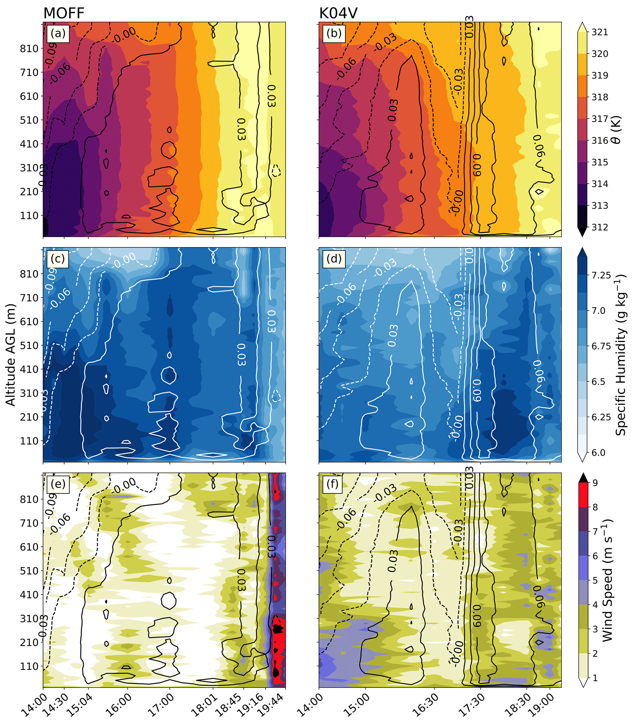
Figure 8Same as Fig. 3 but on 15 July 2018, and panels (a), (c), and (e) are at the MOFF site, and panels (b), (d), and (f) are at the K04V site.
Figure 8c and d show how buoyancy and moisture evolve in time with height at both sites. In the morning, there is more moisture throughout the column at MOFF than K04V. The location of MOFF at the base of the valley leads to more moisture accumulation than within a sloped canyon. At K04V, the drier air near the surface heats more quickly and leads to faster destabilization (Fig. 8b). From 17:00–17:40 UTC, there is a strong positive buoyancy gradient in time at K04V. Here, buoyancy is uniform throughout the entire layer. In addition, low-level moisture increases with time. It is possible this is a result of moisture convergence induced by an outflow from the storms to the north. The strong positive buoyancy aids in the vertical transport of moisture. Rapid destabilization, coupled with deepening low-level moisture, creates a favorable convective environment. Consequently, the K04V ASOS reports 14 m s−1 gusts from 19:54–20:30 UTC. Conversely, at MOFF, there is little change in buoyancy with time, and moisture decreases with time (Fig. 8c), although, at 17:00 UTC, there is vertical transport of moisture accompanied by a layer of increased buoyancy in the lowest 500 m (Fig. 8c). While there appears to be parcel ascent, it was not enough to initiate convection. Once convection begins in the valley (20:00 UTC), MOFF is drier and neutrally buoyant. As a result, the storm favors northward propagation, away from MOFF.
Even though the two sites are only about 27 km apart, there is a difference in how buoyancy evolves in time, showing its spatial sensitivity. Variations in moisture over the two locations change the rate of surface heating. Differences in moisture could be attributed to different land cover or different positions within the valley. Surface conditions influence parcel trajectory, and buoyancy infers deviations about the environmental profile. An increased representation of land–air interactions is a valuable asset to any forecasting tool. Unlike potential temperature, buoyancy is directly impacted by surface conditions at each level of calculation. Buoyancy aligns with changes in moisture where potential temperature does not (Fig. 8c), such that microscale features can be recognized more readily using buoyancy. In Fig. 8c and d, the temperature field at each site is very similar overall, except at 19:30 UTC, when the MOFF site has a cooling throughout the layer by 1 ∘C, likely from the outflow boundary, which the K04V site does not experience (Figs. 7c and 8b). At the time of the rapid increase in buoyancy, the surface temperature at K04V is about 3 ∘C warmer than at MOFF. A shift in surface temperature by a few degrees may be overlooked, but buoyancy accents how that affects the column. Overall, buoyancy in convective settings is sensitive to environmental changes, which may predate the amplification or weakening of convection.
In contrast, Fig. 9a focuses on buoyancy and moisture for a non-CI case that experienced cold-air drainage. Drainage flows are driven by radiative cooling causing the air above the surface to become denser and descend the valley walls. The process continues throughout the night, resulting in a cold pool of air at the base of the valley. Thus, a strong temperature inversion settles in, with subsequent negative buoyancy. The strong easterly winds throughout the early morning confirm a strong downsloping flow (Fig. 9b). Figure 9a quantifies the intensity of stability. Until 14:00 UTC, the stable boundary layer has clearly stratified layers up to 300 m. There is some variability in the vertical extent from 11:33–12:15 UTC, which could be caused by turbulence. It is of note that the region of stratification aligns with a layer of moisture, such that the specific humidity decreases and becomes homogeneous beyond the same height that the buoyancy gradient decreases. Above that level (300 m) and below the stagnation level, there is homogeneous easterly flow (Fig. 9b), all of which suggests a transition to the residual layer. About an hour after sunrise (12:45 UTC), the surface has warmed enough to dilute the density current, which causes the flow to slow within the lowest 100 m (Fig. 9b). Thereafter, the surface warms, and a shallow mixed layer grows, but it is still capped by a stable layer. This region is convectively neutral with an increasing mixed layer depth (Fig. 9a). In the absence of moisture advection, the specific humidity illustrates the vertical mixing. Not until 15:30 UTC is the surface warm enough to initiate the southerly up-valley flow (Fig. 9). This boundary layer transition is unlike either of the other cases examined. Since cold air pools into a thick layer at the base of the valley, the magnitude of stability surpasses what would occur from radiative cooling over flat land. As a result, valley cold pools can lead to persistent fog (Chachere and Pu, 2016). Understanding the timing of mechanical mixing and fog dissipation would aid aviation forecasts.
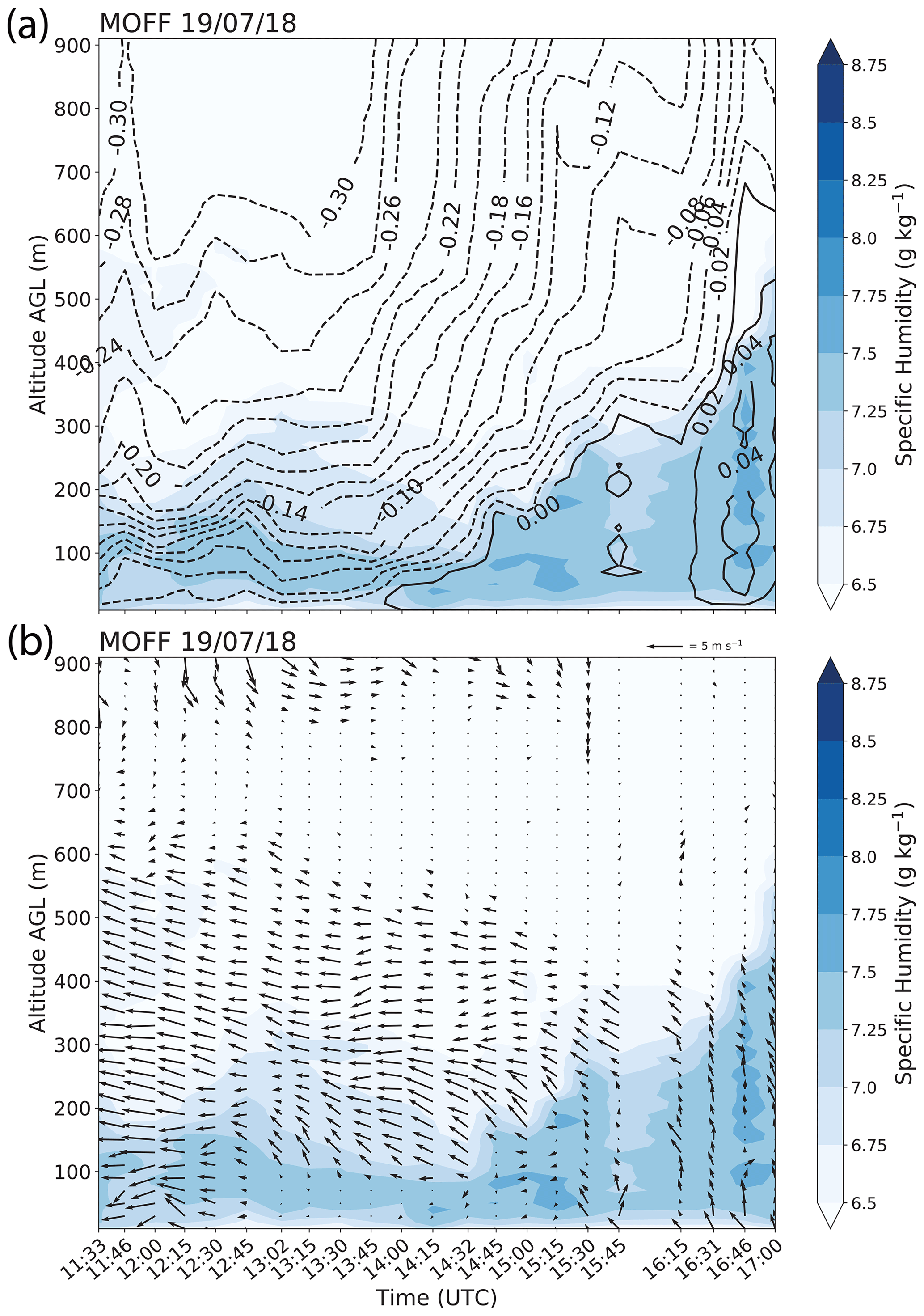
Figure 9(a) Buoyancy contours (m s−2), where solid (dashed) lines are positive (negative) and filled contours are specific humidity (g kg−1). (b) Wind vectors over specific humidity (g kg−1), with filled contours from CopterSonde measurements on 19 July 2018 at MOFF.
This study uses buoyancy measured from RPASs to describe transitions within the ABL. To understand the versatility of using low-level buoyancy, two cases are evaluated. Recent developments in weather sensing RPASs allow for high-frequency sampling within the ABL. The CopterSonde measures at a higher vertical resolution than radiosondes, with comparable accuracy (Figs. 2, 6). Buoyancy has been used prevalently in model studies to interpret microscale to mesoscale processes. The spatial and temporal sensitivity of buoyancy allows for a more detailed interpretation of fine-scale processes. The results show that buoyancy has a diurnal cycle coinciding with the solar cycle (Fig. 6). Buoyancy, like potential temperature, reflects the mixed-layer below the capping inversion, such that the maximum height of constant buoyancy appears to transition with the ABL height (Figs. 3, 8).
The application of vertical buoyancy gradients to derive the ABL height shows promising initial results. The potential temperature- and buoyancy-method-derived heights perfectly correlate (r=1.0) when radiosonde data are used. The correlation from the two methods, using CopterSonde data, is not as strong (r=0.45), although the buoyancy method heights are comparable to the heights derived from the radiosonde data. These heights agree better across methodologies with the radiosonde data than the potential temperature method with different data sources. Inherently, more cases need to be evaluated to have full confidence in the method. Moreover, there are avenues to improve the buoyancy method, particularly when using the CopterSonde data. The high vertical resolution leads to noise in the profiles that is erroneously picked up as the ABL height. Logical arguments will be applied to reduce inconsistencies in ABL heights for consecutive flights. Also, a technique to exclude heights that are beyond the flight ceiling is necessary. The success of this simple method gives credence to the suggestion that, with proper improvements, it could become a trusted ABL height definition.
The two cases show the versatility in buoyancy in different scenarios. While it is beyond the scope of this study to interpret the factors creating the buoyancy gradient, they agree with past findings. Figure 3e and f display a negative buoyancy gradient beginning 2 h before the jet arrives. It is expected that there is a stable boundary layer during nocturnal LLJ (Blackadar, 1957). Moreover, sinking air ahead of the jet would increase stability. As for case 2, Fig. 8b shows an acceleration in positive buoyancy leading up to CI. This agrees with Trier et al. (2014) in the sense that there is rapid destabilization before CI quantified by parcel buoyancy. MOFF has weaker buoyancy (Fig. 8a) and results in shallower convection than K04V. Further investigation is required to see if this is a common occurrence preceding other events.
Real-time sampling allows for data assimilation and improvement in ABL representation for NWP. There is the potential for buoyancy to evaluate many other microscale to mesoscale processes. Measurements taken along a dryline could increase our understanding of where horizontal convective rolls (HCRs) occur. HCRs are conducive for CI due to the vertical motion and thermodynamic gradients described in Weckwerth et al. (1999). Furthermore, understanding cold pool strength and propagation would aid in forecasting severe weather like mesoscale convective systems. Additionally, RPASs can fill a gap in measurements in urban settings to increase our understanding of turbulence and aerosol transport. Buoyant plumes transport aerosols throughout the city, but measuring this typically requires non-permanent towers and tracers such as smoke or colored aerosols. RPASs deployed to determine buoyancy within the urban canopy could help improve air quality predictions. The applications for low-level buoyancy go beyond the topics evaluated in this study. Meanwhile, RPASs can collect measurements during processes that are not easily accessible. Together, they can help address processes not adequately realized.
Regular RPAS profiling opens avenues for increased data assimilation for climate, air quality, and NWP. Buoyancy is just one variable that has shown to be useful in describing the state of the ABL, which was not previously accessible. Buoyancy is sensitive, physical, and simple. Furthermore, remote sensing platforms could use this technique. This study is a simple starting point to revive a classically defined variable in light of new technology. Buoyancy measured by RPASs can describe ABL transitions with little computational power, while providing more information than traditional ABL variables.
Data from the LAPSE-RATE campaign are openly available at https://doi.org/10.5281/zenodo.3737087 (Greene et al., 2020).
Data were collected by TMB, EAPL, and PBC. The data processing and quality control were conducted by TMB. The data analysis and visualization was performed by FML. The paper was written by FML, with contributions from all co-authors.
The contact author has declared that neither they nor their co-authors have any competing interests.
Publisher’s note: Copernicus Publications remains neutral with regard to jurisdictional claims in published maps and institutional affiliations.
Funding has been provided by the NASA University Leadership Initiative (grant no. 80NSSC20M0162). The authors would also like to thank the greater San Luis Valley community, for welcoming the LAPSE-RATE campaign and providing land access for flight operations. Additionally, we thank those CASS members, who gathered and processed the CopterSonde data for both campaigns.
This research has been supported by the National Aeronautics and Space Administration (grant no. 80NSSC20M0162), the National Science Foundation (grant no. 1539070), and the University of Oklahoma Office of the Vice President for Research and Partnerships.
This paper was edited by Laura Bianco and reviewed by David Flagg and two anonymous referees.
Ágústsson, H., Ólafsson, H., Jonassen, M. O., and Rögnvaldsson, Ó.: The impact of assimilating data from a remotely piloted aircraft on simulations of weak-wind orographic flow, Tellus A, 66, 25421, https://doi.org/10.3402/tellusa.v66.25421, 2014. a
Angevine, W. M., Edwards, J. M., Lothon, M., LeMone, M. A., and Osborne, S. R.: Transition periods in the diurnally-varying atmospheric boundary layer over land, Bound.-Lay. Meteorol., 177, 205–223, https://doi.org/10.1007/s10546-020-00515-y, 2020. a, b
Baklanov, A. A., Grisogono, B., Bornstein, R., Mahrt, L., Zilitinkevich, S. S., Taylor, P., Larsen, S. E., Rotach, M. W., and Fernando, H.: The nature, theory, and modeling of atmospheric planetary boundary layers, B. Am. Meteorol. Soc., 92, 123–128, https://doi.org/10.1175/2010BAMS2797.1, 2011. a
Banta, R. M., Pichugina, Y. L., and Newsom, R. K.: Relationship between low-level jet properties and turbulence kinetic energy in the nocturnal stable boundary layer, J. Atmos. Sci., 60, 2549–2555, https://doi.org/10.1175/1520-0469(2003)060<2549:RBLJPA>2.0.CO;2, 2003. a
Barbieri, L., Kral, S. T., Bailey, S. C., Frazier, A. E., Jacob, J. D., Reuder, J., Brus, D., Chilson, P. B., Crick, C., Detweiler, C., Doddi, A., Elston, J., Foroutan, H., González-Rocha, J., Greene, B. R., Guzman, M. I., Houston, A. L., Islam, A., Kemppinen, O., Lawrence, D., Pillar-Little, E. A., Ross, S. D., Sama, M. P., Schmale, D. G., Schuyler, T. J., Shankar, A., Smith, S. W., Waugh, S., Dixon, C., Borenstein, S., and de Boer, G.: Intercomparison of small unmanned aircraft system (sUAS) measurements for atmospheric science during the LAPSE-RATE campaign, Sensors, 19, 2179, https://doi.org/10.3390/s19092179, 2019. a
Båserud, L., Reuder, J., Jonassen, M. O., Kral, S. T., Paskyabi, M. B., and Lothon, M.: Proof of concept for turbulence measurements with the RPAS SUMO during the BLLAST campaign, Atmos. Meas. Tech., 9, 4901–4913, https://doi.org/10.5194/amt-9-4901-2016, 2016. a
Bell, T. M., Greene, B. R., Klein, P. M., Carney, M., and Chilson, P. B.: Confronting the boundary layer data gap: evaluating new and existing methodologies of probing the lower atmosphere, Atmos. Meas. Tech., 13, 3855–3872, https://doi.org/10.5194/amt-13-3855-2020, 2020. a, b, c
Bell, T. M., Klein, P. M., Lundquist, J. K., and Waugh, S.: Remote-sensing and radiosonde datasets collected in the San Luis Valley during the LAPSE-RATE campaign, Earth Syst. Sci. Data, 13, 1041–1051, https://doi.org/10.5194/essd-13-1041-2021, 2021. a
Blackadar, A. K.: Boundary layer wind maxima and their significance for the growth of nocturnal inversions, B. Am. Meteorol. Soc., 38, 283–290, https://doi.org/10.1175/1520-0477-38.5.283, 1957. a
Bonin, T., Chilson, P., Zielke, B., and Fedorovich, E.: Observations of the early evening boundary-layer transition using a small unmanned aerial system, Bound.-Lay. Meteorol., 146, 119–132, https://doi.org/10.1007/s10546-012-9760-3, 2013. a
Braun, S. A. and Tao, W.-K.: Sensitivity of high-resolution simulations of Hurricane Bob (1991) to planetary boundary layer parameterizations, Mon. Weather Rev., 128, 3941–3961, https://doi.org/10.1175/1520-0493(2000)129<3941:SOHRSO>2.0.CO;2, 2000. a
Brown, A. R., Cederwall, R. T., Chlond, A., Duynkerke, P. G., Golaz, J.-C., Khairoutdinov, M., Lewellen, D. C., Lock, A. P., MacVean, M. K., Moeng, C.-H., Neggers, R. a. J., Siebesma, A. P., and Stevens, B.: Large-eddy simulation of the diurnal cycle of shallow cumulus convection over land, Q. J. Roy. Meteor. Soc., 128, 1075–1093, https://doi.org/10.1256/003590002320373210, 2002. a
Chachere, C. N. and Pu, Z.: Connections between cold air pools and mountain valley fog events in Salt Lake City, Pure Appl. Geophys., 173, 3187–3196, https://doi.org/10.1007/s00024-016-1316-x, 2016. a
Chilson, P. B., Bell, T. M., Brewster, K. A., Britto Hupsel de Azevedo, G., Carr, F. H., Carson, K., Doyle, W., Fiebrich, C. A., Greene, B. R., Grimsley, J. L., Kanneganti, S. T., Martin, J., Moore, A., Palmer, R. D., Pillar-Little, E. A., Salazar-Cerreno, J. L., Segales, A. R., Weber, M. E., Yeary, M., and Droegemeier, K. K.: Moving towards a network of autonomous UAS atmospheric profiling stations for observations in the Earth’s lower atmosphere: The 3D Mesonet concept, Sensors, 19, 2720, https://doi.org/10.3390/s19122720, 2019. a
Cohen, A. E., Cavallo, S. M., Coniglio, M. C., and Brooks, H. E.: A review of planetary boundary layer parameterization schemes and their sensitivity in simulating southeastern US cold season severe weather environments, Weather Forecast., 30, 591–612, https://doi.org/10.1175/WAF-D-14-00105.1, 2015. a
Coniglio, M. C., Romine, G. S., Turner, D. D., and Torn, R. D.: Impacts of targeted AERI and Doppler lidar wind retrievals on short-term forecasts of the initiation and early evolution of thunderstorms, Mon. Weather Rev., 147, 1149–1170, https://doi.org/10.1175/MWR-D-18-0351.1, 2019. a
Cuchiara, G. C., Li, X., Carvalho, J., and Rappenglück, B.: Intercomparison of planetary boundary layer parameterization and its impacts on surface ozone concentration in the WRF/Chem model for a case study in Houston/Texas, Atmos. Environ., 96, 175–185, https://doi.org/10.1016/j.atmosenv.2014.07.013, 2014. a
Dai, C., Wang, Q., Kalogiros, J., Lenschow, D., Gao, Z., and Zhou, M.: Determining boundary-layer height from aircraft measurements, Bound.-Lay. Meteorol., 152, 277–302, https://doi.org/10.1007/s10546-014-9929-z, 2014. a, b, c
Dang, R., Yang, Y., Hu, X.-M., Wang, Z., and Zhang, S.: A review of techniques for diagnosing the atmospheric boundary layer height (ABLH) using aerosol lidar data, Remote Sens., 11, 1590, https://doi.org/10.3390/rs11131590, 2019. a, b, c
de Boer, G., Diehl, C., Jacob, J., Houston, A., Smith, S. W., Chilson, P., Schmale, D. G., Intrieri, J., Pinto, J., Elston, J., Brus, D., Kemppinen, O., Clark, A., Lawrence, D., Bailey, S. C. C., Sama, M. P., Frazier, A., Crick, C., Natalie, V., Pillar-Little, E., Klein, P., Waugh, S., Lundquist, J. K., Barbieri, L., Kral, S. T., Jensen, A. A., Dixon, C., Borenstein, S., Hesselius, D., Human, K., Hall, P., Ar- grow, B., Thornberry, T., Wright, R., and Kelly, J. T.: Development of Community, Capabilities, and Understanding through Unmanned Aircraft-Based Atmospheric Research: The LAPSE-RATE Campaign, B. Am. Meteorol. Soc., 101, E684–E699, https://doi.org/10.1175/BAMS-D-19-0050.1, 2020a. a
de Boer, G., Houston, A., Jacob, J., Chilson, P. B., Smith, S. W., Argrow, B., Lawrence, D., Elston, J., Brus, D., Kemppinen, O., Klein, P., Lundquist, J. K., Waugh, S., Bailey, S. C. C., Frazier, A., Sama, M. P., Crick, C., Schmale III, D., Pinto, J., Pillar-Little, E. A., Natalie, V., and Jensen, A.: Data generated during the 2018 LAPSE-RATE campaign: an introduction and overview, Earth Syst. Sci. Data, 12, 3357–3366, https://doi.org/10.5194/essd-12-3357-2020, 2020b. a, b
Degelia, S. K., Wang, X., Stensrud, D. J., and Johnson, A.: Understanding the impact of radar and in situ observations on the prediction of a nocturnal convection initiation event on 25 June 2013 using an ensemble-based multiscale data assimilation system, Mon. Weather Rev., 146, 1837–1859, https://doi.org/10.1175/MWR-D-17-0128.1, 2018. a
De Wekker, S. F., Ameen, A., Song, G., Stephens, B. B., Hallar, A. G., and McCUBBIN, I. B.: A preliminary investigation of boundary layer effects on daytime atmospheric CO2 concentrations at a mountaintop location in the Rocky Mountains, Acta Geophys., 57, 904–922, https://doi.org/10.2478/s11600-009-0033-6, 2009. a
Dias, N., Gonçalves, J., Freire, L., Hasegawa, T., and Malheiros, A.: Obtaining potential virtual temperature profiles, entrainment fluxes, and spectra from mini unmanned aerial vehicle data, Bound.-Lay. Meteorol., 145, 93–111, https://doi.org/10.1007/s10546-011-9693-2, 2012. a
Elston, J., Argrow, B., Stachura, M., Weibel, D., Lawrence, D., and Pope, D.: Overview of small fixed-wing unmanned aircraft for meteorological sampling, J. Atmos. Ocean. Tech., 32, 97–115, https://doi.org/10.1175/JTECH-D-13-00236.1, 2015. a
Flagg, D. D., Doyle, J. D., Holt, T. R., Tyndall, D. P., Amerault, C. M., Geiszler, D., Haack, T., Moskaitis, J. R., Nachamkin, J., and Eleuterio, D. P.: On the Impact of Unmanned Aerial System Observations on Numerical Weather Prediction in the Coastal Zone, Mon. Weather Rev., 146, 599–622, https://doi.org/10.1175/MWR-D-17-0028.1, 2018. a
Gebauer, J. G., Fedorovich, E., and Shapiro, A.: A 1D theoretical analysis of northerly low-level jets over the Great Plains, J. Atmos. Sci., 74, 3419–3431, https://doi.org/10.1175/JAS-D-16-0333.1, 2017. a
Greene, B. R., Segales, A. R., Waugh, S., Duthoit, S., and Chilson, P. B.: Considerations for temperature sensor placement on rotary-wing unmanned aircraft systems, Atmos. Meas. Tech., 11, 5519–5530, https://doi.org/10.5194/amt-11-5519-2018, 2018. a
Greene, B. R., Segales, A. R., Bell, T. M., Pillar-Little, E. A., and Chilson, P. B.: Environmental and sensor integration influences on temperature measurements by rotary-wing unmanned aircraft systems, Sensors, 19, 1470, https://doi.org/10.3390/s19061470, 2019. a, b
Greene, B. R., Bell, T. M., Pillar-Little, E. A., Segales, A. R., Britto Hupsel de Azevedo, G., Doyle, W., Tripp, D. D., Kanneganti, S. T., and Chilson, P. B.: University of Oklahoma CopterSonde Files from LAPSE-RATE (Version v1), Zenodo [data set], https://doi.org/10.5281/zenodo.3737087, 2020. a
Hennemuth, B. and Lammert, A.: Determination of the atmospheric boundary layer height from radiosonde and lidar backscatter, Bound.-Lay. Meteorol., 120, 181–200, https://doi.org/10.1007/s10546-005-9035-3, 2006. a
Houston, A. L. and Niyogi, D.: The sensitivity of convective initiation to the lapse rate of the active cloud-bearing layer, Mon. Weather Rev., 135, 3013–3032, https://doi.org/10.1175/MWR3449.1, 2007. a
Hu, J., Yussouf, N., Turner, D. D., Jones, T. A., and Wang, X.: Impact of ground-based remote sensing boundary layer observations on short-term probabilistic forecasts of a tornadic supercell event, Weather Forecast., 34, 1453–1476, https://doi.org/10.1175/WAF-D-18-0200.1, 2019. a
Hu, X.-M., Nielsen-Gammon, J. W., and Zhang, F.: Evaluation of three planetary boundary layer schemes in the WRF model, J. Appl. Meteorol. Clim., 49, 1831–1844, https://doi.org/10.1175/2010JAMC2432.1, 2010. a
Jonassen, M. O., Ólafsson, H., Ágústsson, H., Rögnvaldsson, Ó., and Reuder, J.: Improving high-resolution numerical weather simulations by assimilating data from an unmanned aerial system, Mon. Weather Rev., 140, 3734–3756, https://doi.org/10.1175/MWR-D-11-00344.1, 2012. a
Jones, T. A., Knopfmeier, K., Wheatley, D., Creager, G., Minnis, P., and Palikonda, R.: Storm-scale data assimilation and ensemble forecasting with the NSSL experimental Warn-on-Forecast system. Part II: Combined radar and satellite data experiments, Weather Forecast., 31, 297–327, https://doi.org/10.1175/WAF-D-15-0107.1, 2016. a
Koch, S. E., Fengler, M., Chilson, P. B., Elmore, K. L., Argrow, B., Andra Jr., D. L., and Lindley, T.: On the use of unmanned aircraft for sampling mesoscale phenomena in the preconvective boundary layer, J. Atmos. Ocean. Tech., 35, 2265–2288, https://doi.org/10.1175/JTECH-D-18-0101.1, 2018. a
Kral, S. T., Reuder, J., Vihma, T., Suomi, I., Haualand, K. F., Urbancic, G. H., Greene, B. R., Steeneveld, G.-J., Lorenz, T., Maronga, B., Jonassen, M. O., Ajosenpää, H., Båserud, L., Chilson, P. B., Holtslag, A. A. M., Jenkins, A. D., Kouznetsov, R., Mayer, S., Pillar-Little, E. A., Rautenberg, A., Schwenkel, J., Seidl, A. W., and Wrenger, B.: The innovative strategies for observations in the arctic atmospheric boundary layer project (ISOBAR): Unique finescale observations under stable and very stable conditions, B. Am. Meteorol. Soc., 102, E218–E243, https://doi.org/10.1175/BAMS-D-19-0212.1, 2021. a
Lapworth, A.: The morning transition of the nocturnal boundary layer, Bound.-Lay. Meteorol., 119, 501–526, https://doi.org/10.1007/s10546-005-9046-0, 2006. a
Lenschow, D., Stankov, B., and Mahrt, L.: The rapid morning boundary-layer transition, J. Atmos. Sci., 36, 2108–2124, https://doi.org/10.1175/1520-0469(1979)036<2108:TRMBLT>2.0.CO;2, 1979. a
Lewis, W. E., Wagner, T. J., Otkin, J. A., and Jones, T. A.: Impact of AERI Temperature and Moisture Retrievals on the Simulation of a Central Plains Severe Convective Weather Event, Atmosphere, 11, 729, https://doi.org/10.3390/atmos11070729, 2020. a
Martucci, G., Matthey, R., Mitev, V., and Richner, H.: Comparison between backscatter lidar and radiosonde measurements of the diurnal and nocturnal stratification in the lower troposphere, J. Atmos. Ocean. Tech., 24, 1231–1244, https://doi.org/10.1175/JTECH2036.1, 2007. a, b
National Research Council: Observing weather and climate from the ground up: A nationwide network of networks, National Academies Press, 2009. a
Nilsson, E., Rannik, Ü., Kumala, M., Buzorius, G., and O’Dowd, C.: Effects of continental boundary layer evolution, convection, turbulence and entrainment, on aerosol formation, Tellus B, 53, 441–461, https://doi.org/10.3402/tellusb.v53i4.16617, 2001. a
Nolan, D. S., Zhang, J. A., and Stern, D. P.: Evaluation of planetary boundary layer parameterizations in tropical cyclones by comparison of in situ observations and high-resolution simulations of Hurricane Isabel (2003). Part II: Inner-core boundary layer and eyewall structure, Mon. Weather Rev., 137, 3675–3698, https://doi.org/10.1175/2009MWR2785.1, 2009. a
Otkin, J. A., Hartung, D. C., Turner, D. D., Petersen, R. A., Feltz, W. F., and Janzon, E.: Assimilation of surface-based boundary layer profiler observations during a cool-season weather event using an observing system simulation experiment. Part I: Analysis impact, Mon. Weather Rev., 139, 2309–2326, https://doi.org/10.1175/2011MWR3622.1, 2011. a
Pal, S., Lee, T., Phelps, S., and De Wekker, S.: Impact of atmospheric boundary layer depth variability and wind reversal on the diurnal variability of aerosol concentration at a valley site, Sci. Total Environ., 496, 424–434, https://doi.org/10.1016/j.scitotenv.2014.07.067, 2014. a
Pillar-Little, E. A., Greene, B. R., Lappin, F. M., Bell, T. M., Segales, A. R., de Azevedo, G. B. H., Doyle, W., Kanneganti, S. T., Tripp, D. D., and Chilson, P. B.: Observations of the thermodynamic and kinematic state of the atmospheric boundary layer over the San Luis Valley, CO, using the CopterSonde 2 remotely piloted aircraft system in support of the LAPSE-RATE field campaign, Earth Syst. Sci. Data, 13, 269–280, https://doi.org/10.5194/essd-13-269-2021, 2021. a, b
Reen, B. P., Stauffer, D. R., and Davis, K. J.: Land-surface heterogeneity effects in the planetary boundary layer, Bound.-Lay. Meteorol., 150, 1–31, https://doi.org/10.1007/s10546-013-9860-8, 2014. a
Reuder, J., Brisset, P., Jonassen, M., Müller, M., and Mayer, S.: The Small Unmanned Meteorological Observer SUMO: A new tool for atmospheric boundary layer research, Meteorol. Z., 18, 141–147, https://doi.org/10.1127/0941-2948/2009/0363, 2009. a
Ruggiero, F. H., Sashegyi, K. D., Madala, R. V., and Raman, S.: The use of surface observations in four-dimensional data assimilation using a mesoscale model, Mon. Weather Rev., 124, 1018–1033, https://doi.org/10.1175/1520-0493(1996)124<1018:TUOSOI>2.0.CO;2, 1996. a
Segales, A. R., Greene, B. R., Bell, T. M., Doyle, W., Martin, J. J., Pillar-Little, E. A., and Chilson, P. B.: The CopterSonde: an insight into the development of a smart unmanned aircraft system for atmospheric boundary layer research, Atmos. Meas. Tech., 13, 2833–2848, https://doi.org/10.5194/amt-13-2833-2020, 2020. a, b
Seibert, P., Beyrich, F., Gryning, S.-E., Joffre, S., Rasmussen, A., and Tercier, P.: Review and intercomparison of operational methods for the determination of the mixing height, Atmos. Environ., 34, 1001–1027, https://doi.org/10.1016/S1352-2310(99)00349-0, 2000. a
Shapiro, A. and Fedorovich, E.: Nocturnal low-level jet over a shallow slope, Acta Geophys., 57, 950–980, https://doi.org/10.2478/s11600-009-0026-5, 2009. a
Shapiro, A., Fedorovich, E., and Rahimi, S.: A unified theory for the Great Plains nocturnal low-level jet, J. Atmos. Sci., 73, 3037–3057, https://doi.org/10.1175/JAS-D-15-0307.1, 2016. a, b, c
Steeneveld, G., Mauritsen, T., de Bruijn, E., Vilà-Guerau de Arellano, J., Svensson, G., and Holtslag, A.: Evaluation of limited-area models for the representation of the diurnal cycle and contrasting nights in CASES-99, J. Appl. Meteorol. Clim., 47, 869–887, https://doi.org/10.1175/2007JAMC1702.1, 2008. a
Stull, R.: 1988: An Introduction to Boundary Layer Meteorology, Kluwer A cademic Publishers, ISBN 9789027727688, 1988. a
Teixeira, J., Stevens, B., Bretherton, C. S., Cederwall, R., Doyle, J. D., Golaz, J. C., Holtslag, A. a. M., Klein, S. A., Lundquist, J. K., Randall, D. A., Siebesma, A. P., and Soares, P. M. M.: Parameterization of the atmospheric boundary layer: a view from just above the inversion, B. Am. Meteorol. Soc., 89, 453–458, https://doi.org/10.1175/BAMS-89-4-453, 2008. a
Trier, S. B., Davis, C. A., Ahijevych, D. A., and Manning, K. W.: Use of the parcel buoyancy minimum (B min) to diagnose simulated thermodynamic destabilization. Part I: Methodology and case studies of MCS initiation environments, Mon. Weather Rev., 142, 945–966, https://doi.org/10.1175/MWR-D-13-00272.1, 2014. a, b
Villa, T. F., Gonzalez, F., Miljievic, B., Ristovski, Z. D., and Morawska, L.: An overview of small unmanned aerial vehicles for air quality measurements: Present applications and future prospectives, Sensors, 16, 1072, https://doi.org/10.3390/s16071072, 2016. a
Wagner, T. J., Klein, P. M., and Turner, D. D.: A new generation of ground-based mobile platforms for active and passive profiling of the boundary layer, B. Am. Meteorol. Soc., 100, 137–153, https://doi.org/10.1175/BAMS-D-17-0165.1, 2019. a
Weckwerth, T. M., Horst, T. W., and Wilson, J. W.: An observational study of the evolution of horizontal convective rolls, Mon. Weather Rev., 127, 2160–2179, https://doi.org/10.1175/1520-0493(1999)127<2160:AOSOTE>2.0.CO;2, 1999. a
Weisman, M. L. and Rotunno, R.: “A theory for strong long-lived squall lines” revisited, J. Atmos. Sci., 61, 361–382, https://doi.org/10.1175/1520-0469(2004)061<0361:ATFSLS>2.0.CO;2, 2004. a
Zhang, Y. and Klein, S. A.: Mechanisms affecting the transition from shallow to deep convection over land: Inferences from observations of the diurnal cycle collected at the ARM Southern Great Plains site, J. Atmos. Sci., 67, 2943–2959, https://doi.org/10.1175/2010JAS3366.1, 2010. a, b
Ziegler, C. L. and Rasmussen, E. N.: The initiation of moist convection at the dryline: forecasting issues from a case study perspective, Weather Forecast., 13, 1106–1131, https://doi.org/10.1175/1520-0434(1998)013<1106:TIOMCA>2.0.CO;2, 1998. a