On the quality of RS41 radiosonde descent data

Radiosonde descent profiles have been available from tens of stations for several years now – mainly from Vaisala RS41 radiosondes. They have been compared with the ascent profiles, with ECMWF short-range forecasts and with co-located radio occultation retrievals. Over this time, our understanding of the data has grown, and the comparison has also shed some light on radiosonde ascent data. The fall rate is very variable and is an important factor, with high fall rates being associated with temperature biases, especially at higher altitudes. Ascent winds are affected by pendulum motion; on average, descent winds are less affected by pendulum motion and are smoother. It is plausible that the true wind variability in the vertical lies between that shown by ascent and descent profiles. This discrepancy indicates the need for reference wind measurements. With current processing, the best results are for radiosondes with parachutes and pressure sensors. Some of the wind, temperature and humidity data are now assimilated in the ECMWF forecast system.

1 Introduction

Radiosondes were first developed in the 1930s and have been used to measure profiles of temperature, humidity and wind since then. There are approximately 800 operational radiosonde stations worldwide, mostly providing ascents once or twice per day. These are used for numerical weather prediction (NWP), climate studies and other applications. The Global Climate Observing System (GCOS) set up the GCOS Reference Upper-Air Network (GRUAN) to produce reference-quality data, with uncertainty estimates, from a subset of stations (Bodeker et al., 2016). Climate users, like GRUAN, tend to focus on temperature and humidity. For NWP, the winds are arguably more important (shown for aircraft data by Ingleby et al., 2021) – partly because satellites provide more temperature and humidity information than wind information. One attraction of radiosonde descent data is that there is very little additional cost involved and potentially an extra vertical profile, assuming that the quality is acceptable. Whilst performing this study, it has become apparent that descent data prompts a re-examination of ascent data, and this can either support or challenge our views of the ascent data.

We have found two previous published studies of radiosonde descent data – with different types of radiosonde. Tiefenau and Gebbeken (1989) compared ascent and descent temperatures and found the descent values to be higher at upper levels. They took the descent temperatures as accurate and suggested that the ascent temperatures were too low due to sampling the balloon wake and adiabatic cooling of the gas within the balloon. Whilst wake effects cannot be completely discounted, our results suggest that the descent temperatures are too high. Using Meisei radiosondes at a station in southern India, Venkat Ratnam et al. (2014) found similar ascent–descent temperature differences and advised some caution when using the descent data; in particular “Note that descent rate is quite high (50–60 m s⁻¹) immediately after balloon burst, and it takes some time to stabilise. Thus, the data within a few kilometers from the balloon burst may be biased because of improper sampling.” Venkat Ratnam et al. (2014) used the radiosonde dimensions to estimate drag and, hence, descent rate; however, there are unknowns (orientation and the mass of the balloon still attached), and the actual descent rates were lower (Fig. 6 in Venkat Ratnam et al., 2014).

As radiosondes are designed to measure during the ascent, it is useful to consider how they differ from dropsondes which always measure on descent. Dropsondes are launched from aircraft and are mainly used for sampling around tropical cyclones and for field experiments. Radiosondes typically have the temperature and humidity sensors mounted diagonally above the radiosonde body, whereas dropsondes (e.g. Hock and Franklin, 1999) have the sensors underneath; in each case, the sensors are placed to sample air undisturbed by the radiosonde body. The AVAPS (Advanced Vertical Atmospheric Profiling System) processing system used by many dropsondes includes an “inertial” correction for the delayed response to horizontal wind shear (Appendix of Hock and Franklin, 1999). Modern radiosondes are usually on a line 30–55 m below the balloon, whereas dropsondes are only 1 m or less below a parachute. As noted by Wang et al. (2008), “The dropsonde fall rate is much smoother than the radiosonde ascent rate because of the radiosonde's pendulum effect and self-induced balloon motion”. Typically dropsondes fall at about 10 m s⁻¹, although it can be about 20 m s⁻¹ just after launch before the parachute opens fully. As discussed below, radiosonde descent can be much faster (to 100 m s⁻¹ or more if no parachute is used) shortly after balloon burst. There has been some use of controlled descent, by partial deflation of the balloon, for measurement of stratospheric humidity (Hurst et al., 2011). Zhang et al. (2019) tested the use of a low-density “hard ball” to give more consistent drag than a parachute when deriving the vertical velocity of the air using a radiosonde descending from a height of about 10 m.

Figure 1 shows BUFR (Binary Universal Form for the Representation of meteorological data) descent reports over Europe for September–November 2019 (descent data were also available from New Zealand, not shown). BUFR allows the reporting of high-vertical-resolution radiosonde data (Ingleby et al., 2016), and Table 1 provides some metadata for them. Geller at al. (2021) found that 44 % of operational radiosonde stations were providing high-vertical-resolution ascent data in mid-2020. Since 2019, descent data have become available from more European stations and a few in the Americas. After launch, the balloon is advected horizontally by the wind, especially at upper levels, and typically travels 50 to 300 km before burst, with the larger distances being more common in winter (Seidel et al., 2011).

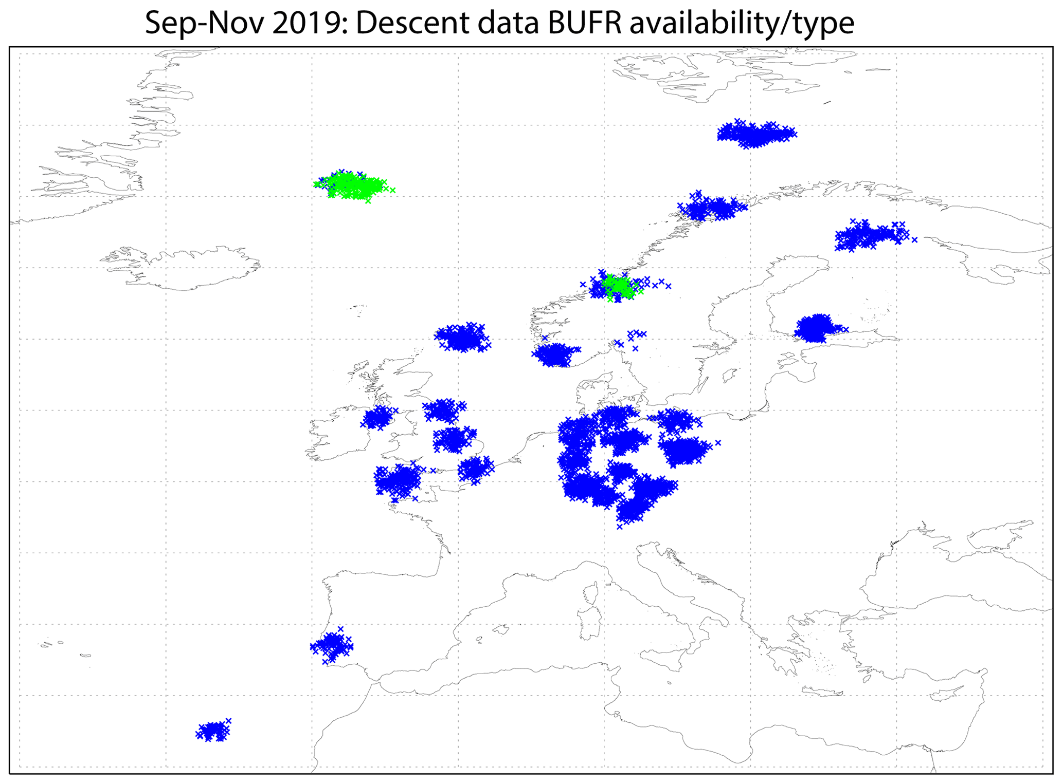
Figure 1 Descent reports (burst positions) over Europe for September–November 2019: blue represents Vaisala RS41, and green represents Modem M10. There were 14 stations from Germany, 6 from the UK and Norway respectively, and 2 from Finland and Portugal respectively.

Figure 2 gives an indication of the number and vertical extent of descent profiles. Larger balloon size and fill volume is used to achieve higher altitudes. On average, radiosondes that achieve higher altitudes drift further horizontally, resulting in the radio signal to the launch station being lost at higher altitudes on descent due to obstruction by terrain or signal attenuation. This can be seen clearly in the UK results which have been split into automatic and manual launches: the manual launches use larger balloons, and the number of descent reports starts to decline earlier (below 9 km). Automatic launchers are documented by Madonna et al. (2020). Some of the other countries use a mixture of manual and automatic launchers but with little or no difference in balloon size. Some ascents, usually less than 5 %, do not have a corresponding descent report, often due to a fault developing with the radiosonde before or upon burst, leading to an automatic termination.

Table 1 Summary of metadata for countries providing descent data in 2019. For balloon weight, the most common value is given; other weights used are given in parentheses, usually with an indication of the stations involved. World Meteorological Organization station identifiers are shown using italic font. The names/locations of the stations can be found at https://oscar.wmo.int/oscar/vola/vola_legacy_report.txt (last access: 4 January 2022). The Czech data were not provided to ECMWF in real time, but they are analysed in Sect. 4.

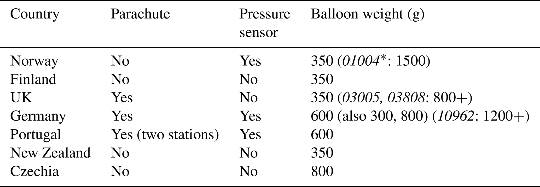
^* Station 01004 did not provide descent reports in 2019.

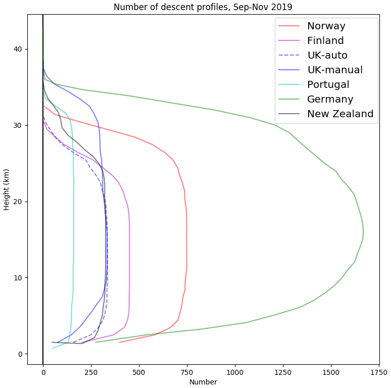
Figure 2 The number of RS41 descent reports by height and country for September–November 2019.

2 Radiosonde ascent and descent

2.1 What goes up must come down

A balloon is filled with hydrogen or helium and ascends, attached by a string to the radiosonde (instrument package). Balloon techniques are documented by WMO (2018b). The Vaisala RS41-SG radiosondes have a small sensor boom with temperature and humidity sensors near the end, and wind and position are measured using a Global Positioning System (GPS) receiver. Some models have a pressure sensor, identified as the RS41-SGP (pressure is discussed in Sect. 4.2). The measurements are transmitted back to the ground station and processed there. Dirksen et al. (2014) describe the GRUAN processing of the Vaisala RS92 and the instrument accuracy; the operational BUFR reports come from the Vaisala processing. The Vaisala RS41 is the successor to the RS92 and is similar in many respects, although with improved humidity and temperature measurements (Edwards et al., 2014; Jensen et al., 2016). As the balloon ascends, it expands in diameter and eventually bursts causing the radiosonde to descend – transmission of the measurements continues but traditionally processing stops at this point. When the radiosonde falls below the horizon as seen from the ground station, it is no longer possible to receive the transmissions. Typically, the ascent takes 90–120 min (reaching altitudes of 30 or 35 km), and the descent takes 30 min or less. The upper part of the descent is close to the upper part of the ascent in both time and space, usually with increasing separation as the radiosonde descends.

Some operators include a parachute, either inside or just below the balloon. The parachute slows the descent and is intended to reduce the risk of damage to life and property when the radiosonde reaches the surface. In sparsely populated or island countries a parachute may not be used.

From rare images of the balloon burst and recovered radiosondes (see Fig. 3 and the Supplement) as well as from the motion on descent, the following is clear: (a) sometimes the balloon bursts completely or tears off at the nozzle and the parachute opens fully; (b) sometimes the balloon tears open leaving strips attached, and these strips may get tangled with the parachute which may partially “free itself” later; (c) sometimes the parachute ruptures and is, thus, ineffective. When there is no parachute, we speculate that the remains of the balloon sometimes act to slow the descent. Note also that, when complete, the mass of the balloon is typically several times that of the radiosonde (larger balloons are used to reach higher altitudes and are also sometimes used at night; the same balloon/amount of gas will reach a higher altitude in the daytime on average). Some stations add extra instruments periodically; for example, once a week, Lerwick (03005) also measures ozone, and a larger balloon and parachute are used.

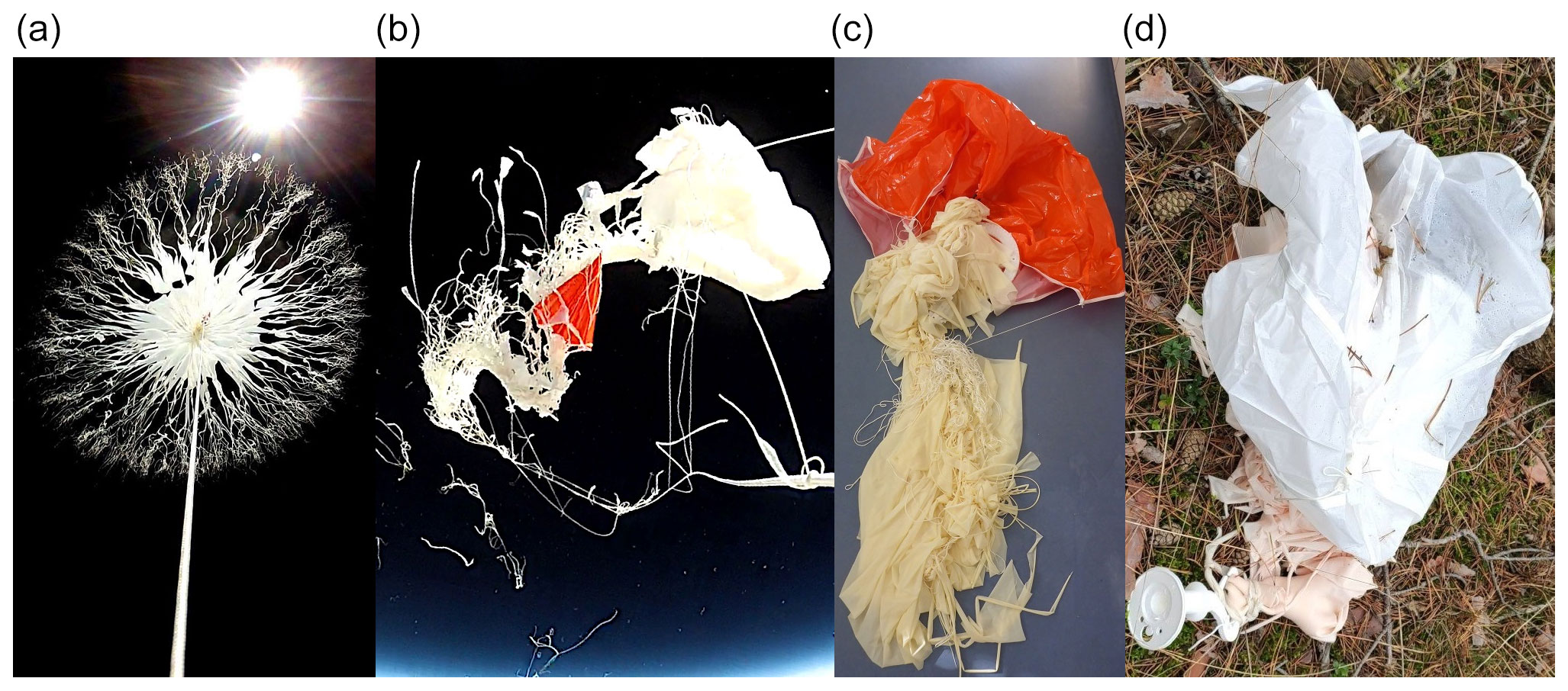
Figure 3 Photographs of (a) a bursting balloon and (b) a parachute (orange) entangled in balloon remains. (c, d) Two images of the balloon remains and parachutes (orange/white) after the descents. These images are for frost point hygrometer launches from Lindenberg; thus, they used larger balloons than a regular radiosonde launch.

On ascent, the sensor boom projects above the radiosonde so that it samples air that has not flowed over the body of the radiosonde. On descent, with a working parachute, it should be in a similar position – so it may sample air that has flowed over the radiosonde body, which has the potential to introduce biases or contamination. It is not known how a radiosonde descending without a parachute is orientated or if it may be tumbling.

2.2 Types of parachute and string length

For some manual launches, a parachute (if used) is attached to the line not far below the balloon. Sometimes the two can become entangled after balloon burst. For automated launches, a parachute (if used) is stored within the balloon, and this seems to cause fewer entanglement problems. This can be used for manual launches too and has been used at Lindenberg for some years, but there is a small additional expense. In general, most of the parachutes are quite basic and do not include a hole. Air can build up inside the parachute and suddenly spill out. It is clear from some of our results that parachutes do not always open as intended.

In earlier decades, the string connecting the balloon and the radiosonde may have been 10 m or less; however, in the stratosphere, the balloon gets larger and there can be intermittent influences of the balloon wake upon the instruments (WMO, 1994; Luers and Eskridge, 1998; Söder et al., 2019). For this reason, longer suspensions are now used, and WMO (2018a) suggests 40 m for radiosondes ascending to 30 km or higher. In practice an “unwinder” is used to increase the line length shortly after the radiosonde launch (WMO, 2018b). The Vaisala unwinder for the RS41 gives 55 m when extended (Vaisala, 2017a). We note that while longer lines benefit stratospheric temperature measurements, they cause larger-amplitude pendulum motion in the winds.

2.3 Preparation of profile reports

Data values are transmitted to the ground receiver every second and are processed by Vaisala MW41 software. Raw data values, both ascent and descent, indexed by time are stored locally (the GRUAN archive makes the 1 s data available for GRUAN sites). The MW41 software looks for a sustained decrease in altitude to determine the time of burst. In the past, all later data would usually have been discarded, but there is now an option to continue processing and to produce a separate BUFR descent message using sequence 3 09 056 (WMO, 2021) designed for descent data. In 2019, as an interim measure, the dropsonde sequence 3 09 053 was being used. As the timeliness of ascent data is critical for data users, it is preferable to transmit the ascent profile as soon as possible after burst, followed by the descent data sent once the profile is completed. BUFR from the European stations involved in this study is generally provided every 2 s (about 10 m separation in the vertical during ascent).

The MW41 horizontal winds are derived primarily from Doppler processing of the GPS signals, but the GPS locations are also used (GRUAN processing only uses the GPS positions). There is very good vertical resolution, but it also means that the winds sample the pendulum motion of the radiosonde – this is probably a mixture of planar and conical pendulum motion. The period of the pendulum motion is a function of the length of line between the balloon or parachute and the radiosonde. The processing attempts to filter out the pendulum motion (discussed briefly in Dirksen et al., 2014), but the filtering is imperfect as discussed below.

2.4 Descent fall rates

The balloon and gas are chosen so that the ascent rate is about 5 m s⁻¹ on average; however, there is usually notable high-frequency variability, probably due to pendulum motion. Especially in the stratosphere, there can be lower-frequency signals due to gravity waves, and both of these features can be seen in Fig. 4 (grey line, ascent). After the balloon bursts, the radiosonde falls very fast (over 70 m s⁻¹ in this case) and then slows abruptly – presumably when the parachute opens fully. After this, there is a little high-frequency variability (but much less than on the ascent) and a gradual decrease in descent rate as the air density increases. Looking at a sample of Lindenberg descents over several weeks (see the Supplement), some exhibit an abrupt deceleration and others do not. Figure 5 shows descent rates from the station at Sola in Norway, without parachutes. These do not show the abrupt deceleration, but they do show a large range of descent rates. The slower descents tend to have larger high-frequency variability. In these cases, we tentatively suggest that the remains of the balloon are acting to slow the descent and that there is some pendulum motion. Venkat Ratnam et al. (2014) suggested that the balloon remains sometimes act as a parachute. The variability in the descent rate may be due to variability in the mass and shape of balloon remnants.

Figure 4 Ascent (grey) and descent (red) rate – an example from Lindenberg (1 s data).

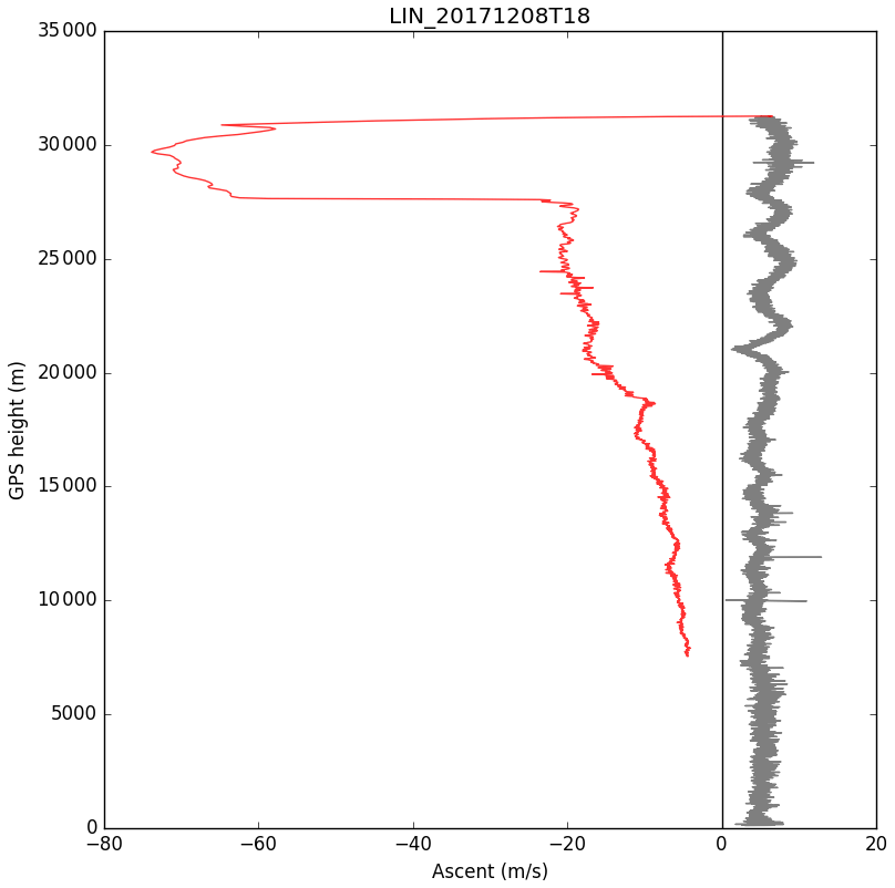
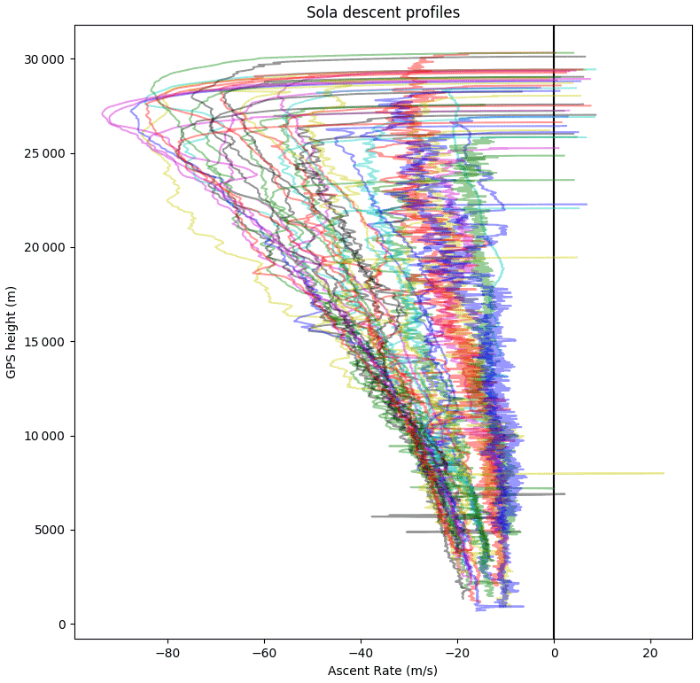
Figure 5 Descent profiles from Sola, Norway (data courtesy of Terje Borge) for 14 December 2019–5 January 2020.

Mean descent rates by country are shown in Fig. 6 (an indication of the variability is shown for Germany). For any particular altitude, mean decent rates from Germany and the UK are the slowest, reflecting their use of parachutes. Amongst the others, there is a large range. The Norwegian radiosondes fall faster than those from the other countries studied – it is unclear why they fall faster than the Finnish radiosondes. In Sect. 3, we focus on the four northern European countries (Norway, Finland, the UK and Germany) because they have similar upper-air climatologies but different instrument characteristics. For Germany and Finland, the descent data received at ECMWF stopped on about 20 November 2019 linked to the move to the new BUFR template. During 2020, the volume of descent profiles increased overall (e.g. France and Spain started sending them), although there was also some disruption from the Covid pandemic.

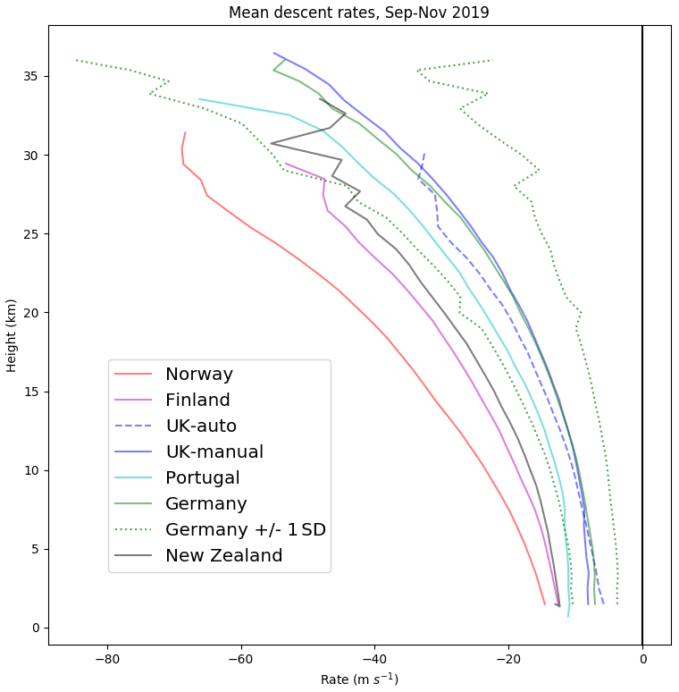
Figure 6 Mean descent rates for September–November 2019, showing the same categories as Fig. 2. For German profiles, an indication of the standard deviation (SD) has been provided.

2.5 Motion of radiosonde during descent

As it ascends through the atmosphere, a radiosonde can be thought of as a pendulum with a moving pivot (Marlton et al., 2015). As the radiosonde encounters small-scale turbulence, which is ubiquitous in our atmosphere, it causes the radiosonde beneath to swing. The periodicity τ is a function of string length l given by

$$\begin{array}{}\text{(1)}& \mathit{\tau }=\mathrm{2}\mathit{\pi }\sqrt{{\displaystyle \frac{l}{g}}},\end{array}$$

where g is the acceleration due to gravity. Different radiosonde manufacturers supply different string lengths for their radiosondes, with the aim of removing the radiosonde sensors from the wake effects (Luers and Eskridge, 1998). The standard string length on the Vaisala RS41 is 55 m (Vaisala, 2017a) and gives an approximate period of oscillation of 14.9 s and an oscillating frequency of approximately 0.07 Hz. Differing balloon sizes and the inclusion of a parachute may alter l and, therefore, τ slightly: a ±5 m variation of l affects τ by ±0.7 s. Given the non-linear relationship in Eq. (1), a similar length addition for a radiosonde with a shorter tether, for example, will have a larger change on the period of oscillation. Depending on the operating practices, the radiosonde may be launched in three broad configurations: (i) no parachute – the radiosonde free-falls with some drag from the balloon remnants; (ii) balloon bursts above the parachute and the radiosonde descends on the parachute; and (iii) the balloon contains a parachute which then deploys above the neck of the balloon and similarly descends. In addition to this, the deployment of the parachute is not consistent (see Figs. 4, S4 and S5).

Marlton (2016) performed a spectral analysis of raw GPS wind measurements from Vaisala RS92 radiosonde ascents equipped with motion sensors described in Harrison and Hogan (2006) and Marlton et al. (2015) and found that oscillatory modes detected by the motion sensors were present in the raw GPS data. In this section, raw GPS ascent and descent data from UK Met Office autosonde sites and from manually operated stations are used to generate Lomb periodograms of the raw horizontal wind components.

Due to radiosondes often travelling 4–5 times their vertical ascent height in the horizontal, there are small data gaps on occasion due to transmission dropout. The issue becomes more noticeable in descent data, as the radiosonde is now even further from its ground station. This means that a traditional Fourier transform method is not appropriate. Thus, a Lomb periodogram, which can generate periodograms that have irregularly sampled data, is chosen (Lomb, 1976). To ensure that we focus on the motion of the radiosonde, we use the processed horizontal wind components to remove the wind field from our raw GPS readings, leaving the motion of the radiosonde beneath that balloon.

Figure 7a–d shows Lomb periodograms of the detrended horizontal GPS components during an ascent for four different RS41 launch configurations; in each case there is a dominant oscillatory period of 15 s (0.06 Hz) which strongly dominates above 15 km. Examining the results from Eq. (1) given the RS41's string length shows that the radiosonde and balloon are behaving as a pendulum with a moving pivot on ascent.

Figure 7 Composite Lomb periodograms of detrended horizontal GPS data as a function of height for ascent data from RS41s with the following launch configurations: (a) TX350 balloon with internal parachute, (b) TX500 with no parachute, (c) TX1200 with external parachute (daytime only) and (d) TX800 with external parachute. Panels (e)–(h) show composite Lomb periodograms of descent data from the balloon configurations shown in panels (a)–(d) respectively. Profile contributions for the balloon configurations in panels (a)–(d) during ascent (descent) are shown in black (red) in panels (i)–(l) respectively.

During descent, the oscillatory motion is very different: there is no longer a dominant oscillatory period and the amplitudes of these oscillations are smaller. A general trend is that the radiosonde is still oscillating with a period of 15 s (0.06 Hz) in the early stages of the descent. As it falls, the peak period of oscillation increases to 25–30 s until a height of 15–20 km. At this approximate height, the RS41s without parachutes (Fig. 7e) exhibit a narrow spectral width with the smallest descent to descent variability. However, an oscillation is still present, indicating that some of the balloon remnants are acting as a parachute. For the parachuted RS41s, the spectral width in oscillation widens significantly, indicating that there is variation in the motion behaviour of the radiosonde. As discussed earlier, this may be due to how and when the parachute deployed and if any of the parachute remains entangled with the parachute rigging. The latter is hard to determine without retrieving the radiosonde, which is seldom done. We can get a better understanding of the variation in oscillation by looking at individual ascents.

Figures 8 and 9 show two descents from Castor Bay autosonde station (54.50^∘ N, 6.34^∘ W). Figures 8a and 9a show the processed horizontal wind components u and v components in red and blue respectively. The raw GPS wind components are shown in black and orange for the u and v components respectively. Figures 8b and 9b show the descent speed and Fig. 8c and d and Fig. 9c, d show Lomb periodograms of the detrended raw GPS velocities. In Fig. 8, we see that the parachute does not seem to offer significant deceleration to the sonde until about 14 km, and there are also weak low-frequency oscillations with a period greater than 60 s over the duration of the descent. In Fig. 8a, the raw GPS data and the processed v component of the wind track very closely, and it is hard to differentiate between them. Figure 9 is a descent from a different day which tells a very different story. The parachute deploys within 1 km of the burst height and causes a sudden deceleration from −60 to −20 m s⁻¹. After the rapid deceleration, the radiosonde enters a high-amplitude oscillatory mode with a periodicity of 30–40 s as it descends. A hypothesis here is that the sudden deceleration caused by a correct deployment of the parachute has generated the observed oscillatory mode. The amplitude of oscillations seen under this scenario could introduce error in the processed winds and is a possible area for future study, as is the optimal filtering for descent winds.

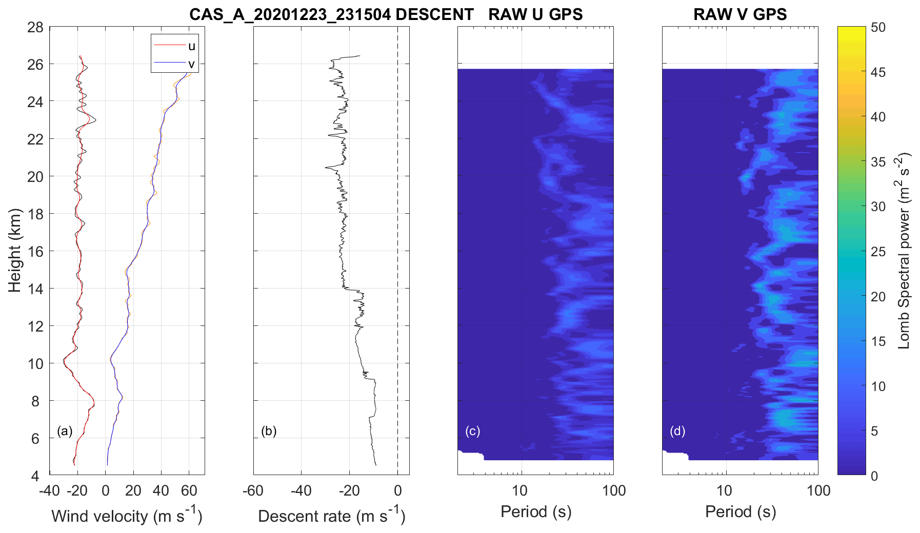
Figure 8 Vertical profiles of (a) processed horizontal wind components u and v in solid red and blue respectively with raw GPS winds in black and orange for the u and v components respectively, and (b) descent speed. Panels (c) and (d) show Lomb periodograms of the detrended raw GPS velocities as a function of height for a sounding made at Castor Bay autosonde station (54.50^∘ N, 6.34^∘ W) at 23:15 UTC on 23 December 2020.

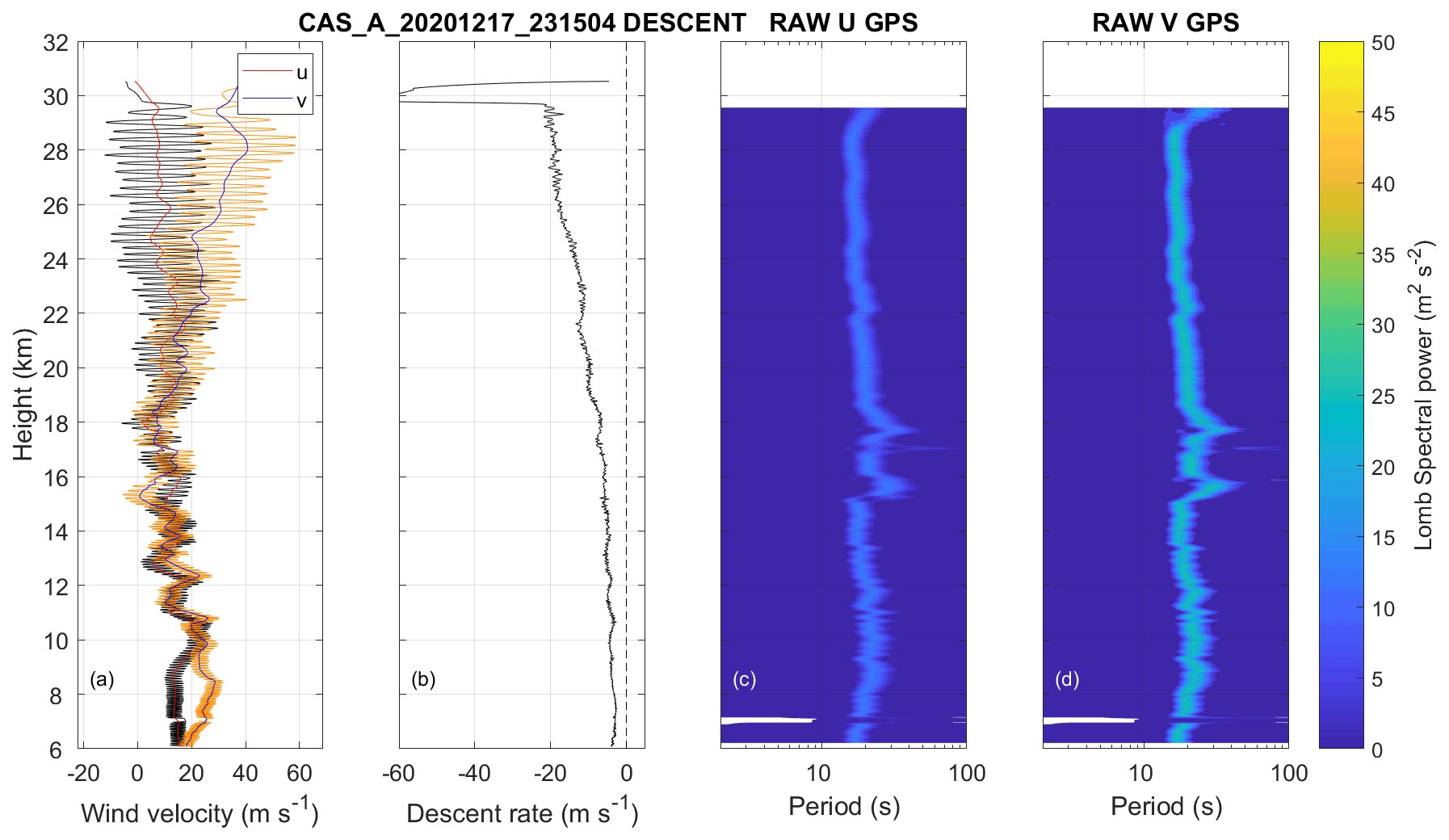
Figure 9 Vertical profiles of (a) processed horizontal wind components u and v in solid red and blue for respectively with raw GPS winds in black and orange for the u and v components respectively, and (b) descent speed. Panels (c) and (d) show Lomb periodograms of the detrended raw GPS velocities as a function of height for a sounding made at Castor Bay autosonde station (54.50^∘ N, 6.34^∘ W) at 23:15 UTC on 17 December 2020.

Here, it has been shown that identical balloon configurations have very different and random descent characteristics. Figure 3 shows that the balloon sometimes twines itself about the parachute which may affect how well the parachute deploys and, in turn, its oscillatory characteristics on descent. A successful parachute deployment can enhance the oscillation such that it has potential to introduce error in descent wind data, depending on the size of the averaging window used by the sounding software. More research in this area needs to be undertaken using an approach where motion sensors are attached to the RS41 to better understand the descent-to-descent variability. Additional investigations where guillotines cut the balloon from the parachute, such as those used on heavy scientific balloon payloads, could be utilised to remove the effect of balloon entanglement. The placement of a small central hole in the top of the parachute to improve stability and removal of sudden deceleration also requires investigation.

In summary, ascending radiosondes tend to have similar characteristics in terms of motion beneath the balloon and ascent speeds, although the latter depends on the amount of gas within the balloon. Descending radiosondes have widely varying descent characteristics which are due to the random nature of how the balloon and parachute interact (if present) and how effective the parachute is at slowing the balloon. The motion on descent may be more consistent if the radiosonde could be “cut free” of the balloon remains and fall on its own without a parachute. It would be interesting to study the effect of cutting the string just after balloon burst, but this may be technically difficult and the risk associated with the radiosonde falling at terminal velocity would need to be assessed. Given the variation in burst heights, reliably cutting the balloon free before burst would reduce the average height attained. In addition, similar motion and orientation sensors to those used in Harrison and Hogan (2006) and Marlton et al. (2015) could be used to ascertain more information about the orientation of the descending radiosonde package.

3 Comparison with ECMWF background fields

3.1 The ECMWF forecasting system

For comparison, we use statistics from the ECMWF operational data assimilation system for September to November 2019. The forecast model had a horizontal grid spacing of about 9 km and 137 levels in the vertical, and the assimilation used 4D-Var with a 12 h window. The respective 3–15 h forecast periods from the previous analysis form the background for the assimilation, and the observation minus the background (O − B) statistics can yield a lot of information. The background values are not perfect but provide a relatively accurate and (generally) independent estimate of the measured variables. In many respects, the forecasting system is similar to that of ERA5 (Hersbach et al., 2020), which was based on the operational system of 2016. One difference from ERA5 is that treatment of radiosonde drift was introduced operationally in June 2018, and this improved upper-level O − B standard deviations (SDs) by 5 %–10 % (Ingleby et al., 2018). Prior to this, radiosonde profiles were treated as vertical and instantaneous. Afterwards, and in this study, ascent profiles were split into sub-profiles of 15 min each and treated as valid at the time and latitude/longitude of the first point in the sub-profile. Descent profiles are split into 5 min sub-profiles for comparison with the model.

3.2 Wind comparison

Figure 10 shows mean and standard deviation (SD) profiles of O − B differences at radiosonde standard levels for the u (zonal) component of the wind. The statistics for the v (meridional) component are similar and are not shown. The mean differences (dashed lines) are close to zero, as hoped. The standard deviations are approximately 2 m s⁻¹, but they are slightly larger at the top levels. One surprise was that the descent profiles (in red) fit the variations in background wind more closely than the ascent profiles (in black), particularly at upper levels. Comparing individual ascent and descent profiles, the descent winds generally appear smoother, and this appears to be the cause of the better fit to background. This is illustrated in Fig. 11, which shows the raw 1 s data for a single profile (faint line) and the data after smoothing to remove the pendulum motion (bold line). In this case, the smoothing was performed using the GRUAN algorithm (Dirksen et al., 2014), whereas the BUFR reports have smoothing applied by Vaisala MW41 software which is similar but not identical. In both cases, a time filter with a fixed window is applied to all profile data. Improvements to this are possible, as is clear from Sect. 2.5. Because the radiosonde is falling faster than it ascended, a filter based on a fixed time interval corresponds to a larger height interval on the descent. Note also that the MW41 processing does not include an inertial correction as used in the AVAPS dropsonde processing (Sect. 1), which would counteract time-lag effects that are largest when falling fastest. As shown in Fig. 11 (also Figs. S6 and S7), there is less high-frequency “pendulum” motion on the descent at most levels – although there can be substantial amounts of noise at the top levels.

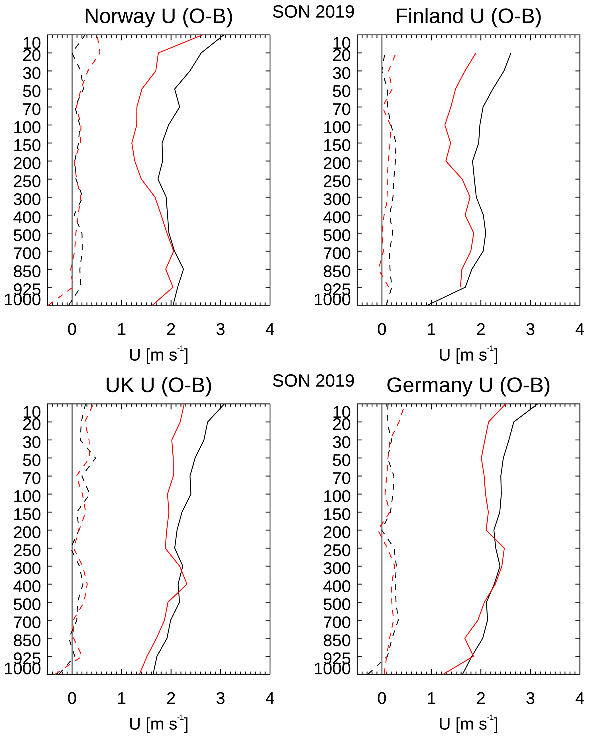
Figure 10 The u-component standard level statistics of the mean (dashed) and standard deviation (SD; solid) O − B differences for ascent (black) and descent (red) for four different countries for the period from September to November 2019.

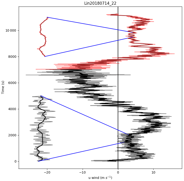
Figure 11 The raw (1 s) data (pale line) and the filtered (bold line) u component as a function of time for ascent (black) and descent (red). This is for a launch from Lindenberg, including a parachute for the descent. Two sections are shown in more detail with the time axis scaled by 10.

Figure 12 shows the SD of O − B for individual descents in the interval from 30 to 50 hPa against the mean descent rate for this pressure range. The standard deviations are slightly larger for slower descent rates, which is thought to be linked to larger-amplitude pendulum motion when the parachute is slowing the descent more effectively. Similar effects can be seen for other pressure ranges, but there is no clear dependence of the mean (O − B) winds on descent rate (not shown).

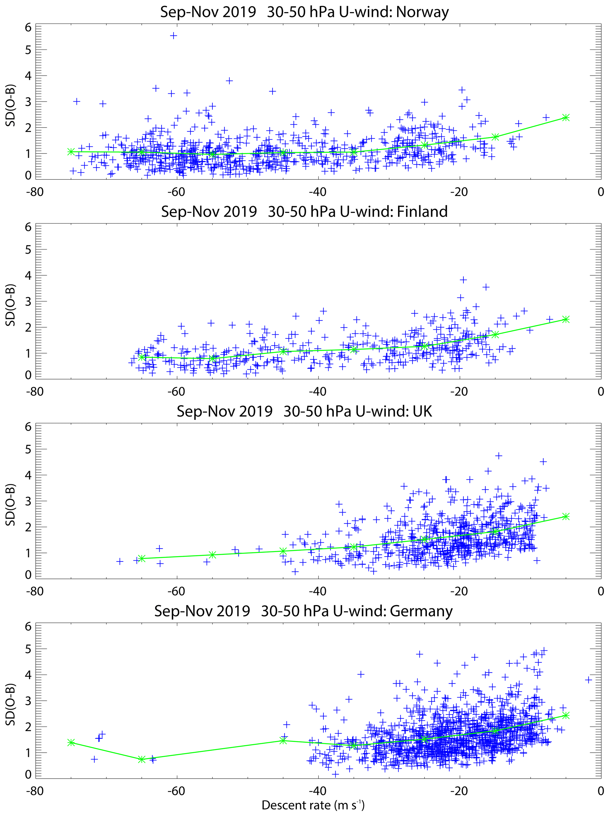
Figure 12 The standard deviation of O − B plotted against the mean descent rate, both for descents from 30 to 50 hPa (blue symbols). The green symbols show the average values for bins of 10 m s⁻¹.

3.3 Temperature comparison

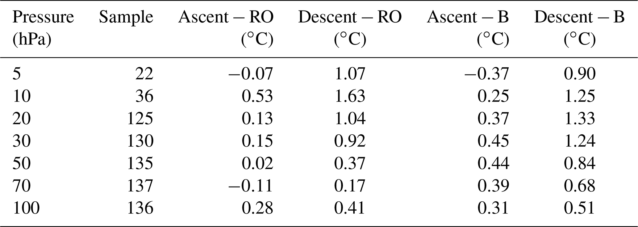
Firstly, we note that the ECMWF background is about 0.5 ^∘C too cool at approximately 50 hPa, in the extratropics (this can be seen against the RS41 ascent data in Fig. 13). This is recognised as a model error, due mainly to excessive humidity and, hence, extra long-wave cooling, as shown by Shepherd et al. (2018). More recent work on the analysis system has approximately halved the short-range forecast bias (Laloyaux et al., 2020); they included comparison against radio occultation (RO) retrievals. We compared radiosonde ascent–descent pairs with RO retrievals that were within 100 km and 2 h of the burst point (Table 2). The RO data are much closer to the ascent temperatures than the descent temperatures; note that the sample size is much smaller than for the O − B statistics (137 versus 2190 at 70 hPa).

Table 2 Co-locations with radio occultation (RO) retrievals (within 100 km and 2 h) for all stations at standard levels, with mean temperature differences (^∘C). Columns show radiosonde ascent (or descent) minus RO or background (B) values; the comparisons with the background are limited to the profiles co-located with RO.

Figure 13 Figure 13 is the same as Fig. 10 but for temperature.

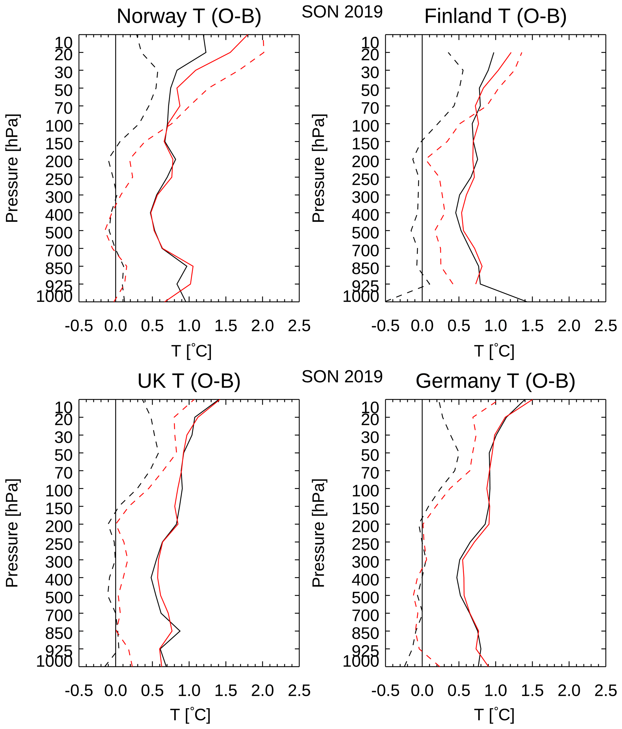
The clearest difference between ascent and descent is that, at upper levels, the descent temperatures are higher than the ascent values (Fig. 13). This has been noted previously for different radiosonde types (see Sect. 1). At 10 hPa, the descent − ascent difference is over 1.5 ^∘C for the Norwegian stations and about half that for the UK and German stations. For Finland, the highest standard level reached is generally 20 hPa, and the difference there is about 1 ^∘C. One hypothesis advanced was that this could be a time-lag effect. The temperature sensor response time at a 6 m s⁻¹ flow is 0.5 s at 1000 hPa, 1.2 s at 100 hPa and 2.5 s at 10 hPa (Vaisala, 2017b). (For a higher flow speed, the response time is shorter. RS41 temperature data are corrected for time lag in both the ascent and descent phases.) However, descending from 30 to 100 hPa, the mean temperatures over northern Europe were approximately constant or increased slightly (not shown), suggesting that another explanation is needed. A convincing link to the radiosonde fall speed was found (Fig. 14). There is no clear link to the time of day (and solar radiation), as shown by the different coloured symbols in Fig. 14. The SD of O − B for temperature shows no clear link to fall rate (not shown).

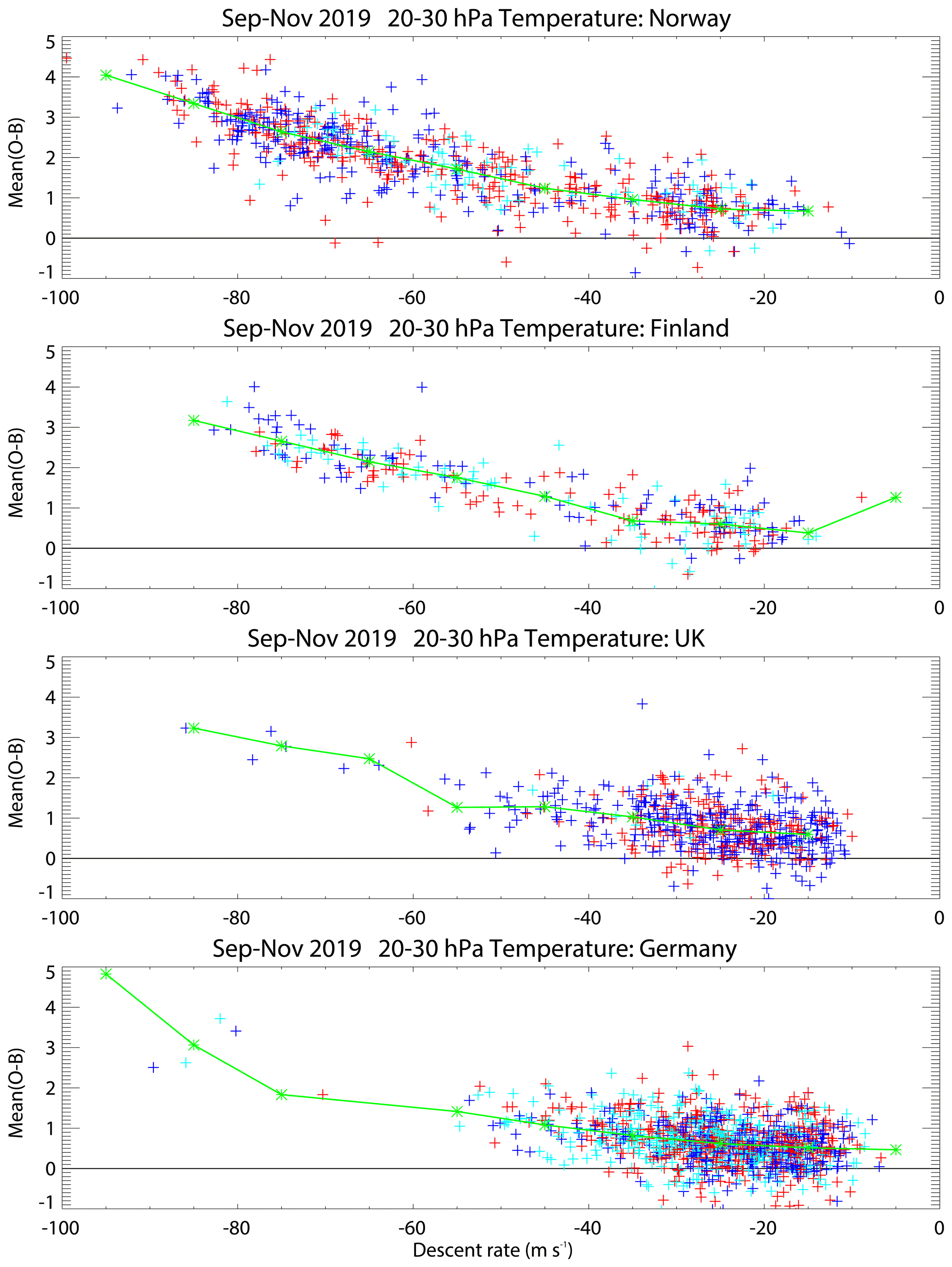
Figure 14 Comparison between the mean fall speed from 20 to 30 hPa and the mean O − B temperature. Red markers denote nominal 12:00 UTC profiles, dark blue markers denote nominal 00:00 UTC profiles and cyan denotes intermediate profiles. (Recall that the B values have a bias of about 0.4 ^∘C at these levels.) Green markers show the values averaged over all times of the day in bins of 10 m s⁻¹.

Returning to Fig. 13, the large top-level ascent–descent difference in the Norwegian data disappears below 300 hPa, but the smaller top-level Finnish difference becomes an offset of 0.2 or 0.3 ^∘C throughout the troposphere. The important difference seems to be that the Norwegian radiosondes have a pressure sensor, but the Finnish radiosondes do not. Without a pressure sensor, the pressures must be computed, and biases in the temperature will feed into later biases in the pressures, as discussed in more detail in the next section. A smaller version of the same effect can be seen between the German data (with pressure sensors) and the UK data (without a pressure sensor); the latter data have an offset of about 0.1 ^∘C in the troposphere, which is smaller than the Finnish offset because the UK radiosondes have parachutes.

3.4 Humidity comparison

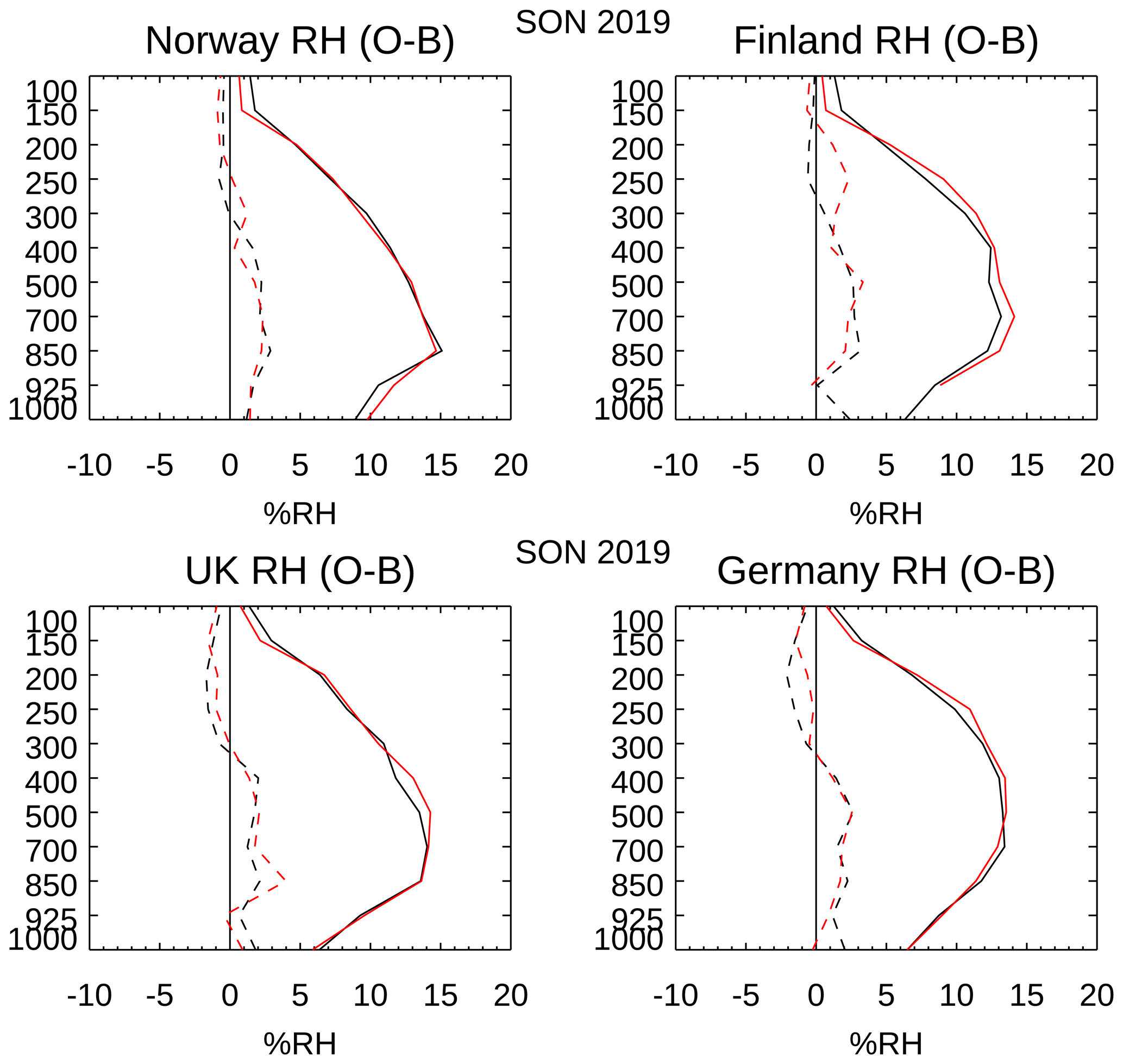
Figure 15 shows ascent–descent comparisons with the background for relative humidity (RH) (see the Supplement for specific humidity). Broadly speaking, the ascent and descent statistics are very similar, although the descent fit to background is slightly worse for the Finnish radiosondes in the troposphere. Between about 50 and 150 hPa, the SD of O − B for RH is smaller for the descent, but it should be noted that stratospheric radiosonde humidity is not assimilated in the ECMWF nor in other NWP systems.

Figure 15 Figure 15 is the same as Fig. 10 but for relative humidity – up to 100 hPa.

4 Warm bias during descent

4.1 The direct effect of heating

As the comparison of descent data with an NWP model suggests, there is a positive temperature bias in the data measured by descending Vaisala RS41 radiosondes. This bias is bigger in the stratosphere than in the troposphere and is more significant for the data taken from radiosondes without parachutes.

As the descent rate often exceeds 50 m s⁻¹, occasionally even 100 m s⁻¹, frictional heating seems to be a reasonable explanation of the observed bias. A related issue is recognised for sensors on aircraft, which also measure temperature while moving fast relative to the free air (WMO, 2018b, Sect. 3.3). For aircraft, the kinetic energy is transferred to internal heat, mostly by adiabatic compression. For radiosondes, we expect that most of the conversion is done by direct collisions of air and sensor molecules (friction), but it is also possible that the effect is done by adiabatic compression in the boundary layer of the sensor. We use a quadratic relationship on descent rate (DR) – this arises from a simple energy balance, independent of the energy conversion mechanism:

$$\begin{array}{}\text{(2)}& \mathrm{\Delta }T=A{\mathrm{DR}}^{\mathrm{2}},\end{array}$$

where A is a coefficient, determined below. This is similar to the equation for the heating of aircraft temperature sensors (see the Appendix). It is also linked to the “viscous dissipation” or “compressional heating” mentioned by Wagner (1964) for rocketsondes. (Launched high in the atmosphere by a rocket, rocketsondes measure on the descent and are slowed by a parachute.) This relationship was examined by comparing the descent temperatures with ascent temperatures from the same radiosonde. Most of the data were from the Praha-Libus (Prague) upper-air station: three launches per day, 554 descents with average length of descent 23 km; there were about 528 000 points at which ascent and descent could be compared. The data cover the period from July 2019 to January 2020, using RS41-SG radiosondes without a pressure sensor or parachute (as for the Finnish soundings above).

The time and space difference between ascent and descent at a particular level is zero at balloon burst and can rise to 2 h and 150 km for lower tropospheric levels. This difference will result in deviations of atmospheric measurements. In Sect. 3, the model values (including the model diurnal cycle) are subtracted from the radiosonde temperatures, but comparing ascent and descent directly samples the diurnal cycle. There is little diurnal cycle at upper levels, but we expect to see mean descent − ascent differences below 4 km due to the diurnal variation and time difference.

For each point we have height (H), descent rate (DR) and descent temperature (T_D), with ascent temperature (T_A) interpolated to this level. After dividing the sample into bins of 1000 m in altitude, the bias was calculated (mean temperature difference $\mathrm{\Delta }T=T_{\mathrm{D}}-T_{\mathrm{A}}$) for each bin. The results shown in Fig. 16 are very similar to the comparison of German data shown in Fig. 13 – about a 1 ^∘C bias at the highest levels decreasing to 0 ^∘C at 12 km. The low-level descent − ascent differences are −0.4, 0.2 and 1.1 ^∘C for the 00:00, 06:00 and 12:00 UTC profiles respectively, reflecting the diurnal cycle and giving a positive bias overall.

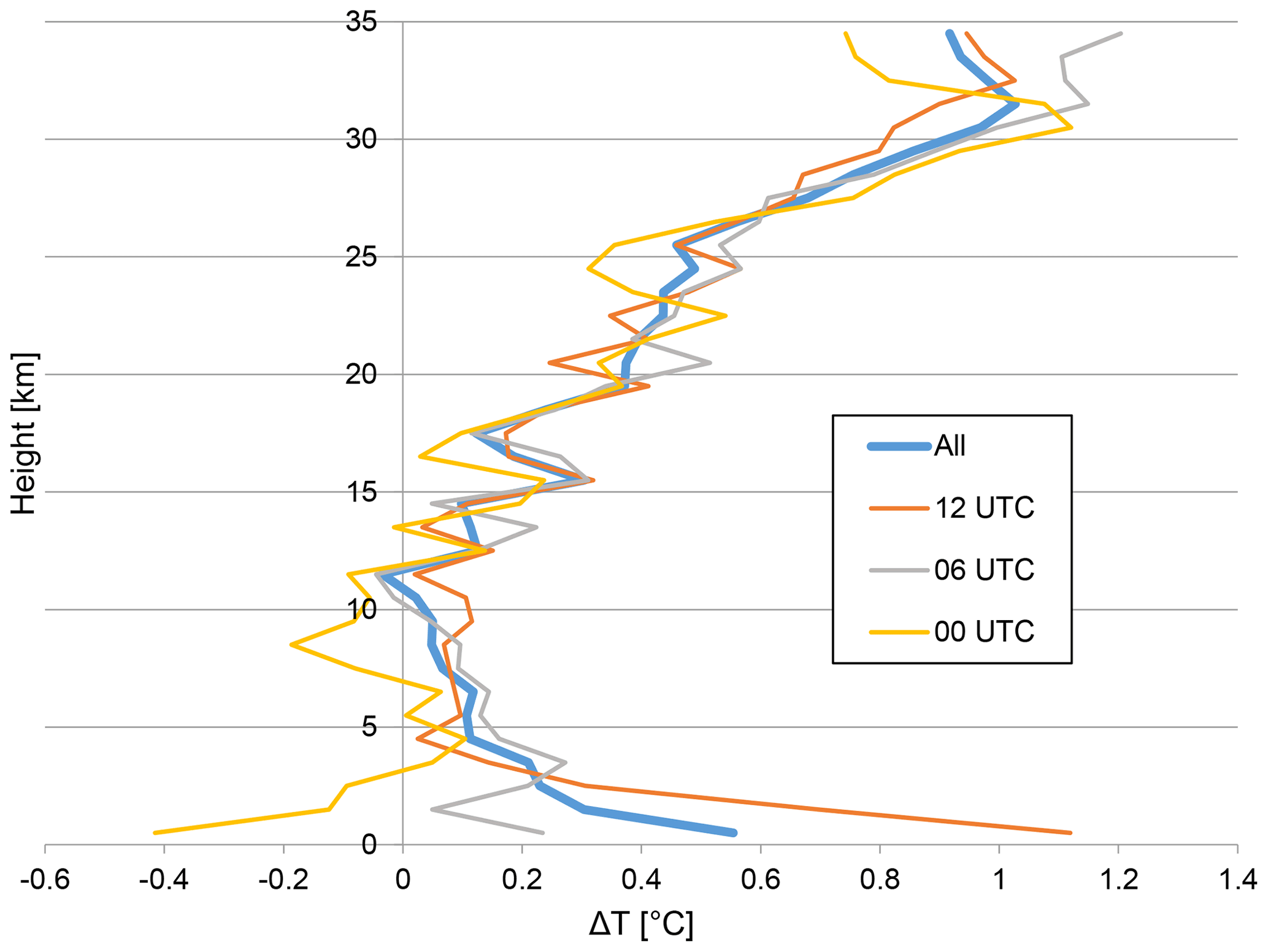
Figure 16 The temperature differences between ascent and descent as a function of height (Praha-Libus data).

According to Eq. (2), ΔT should depend solely on DR. The Pearson correlation coefficient confirms the strong link between these two variables. It was 0.21 between ΔT and H and 0.40 between ΔT and DR.

In the next step, the sample was binned by DR – the intervals used were 0–5, 5–10 m s⁻¹ and so on. There is clearly a quadratic dependence of ΔT on DR in Fig. 17 (average ΔT for these bins). The standard deviation of ΔT, shown using grey lines, is almost independent of DR. The black line is the best estimate with $A=\mathrm{4.05}\times {\mathrm{10}}^{-\mathrm{4}}$.

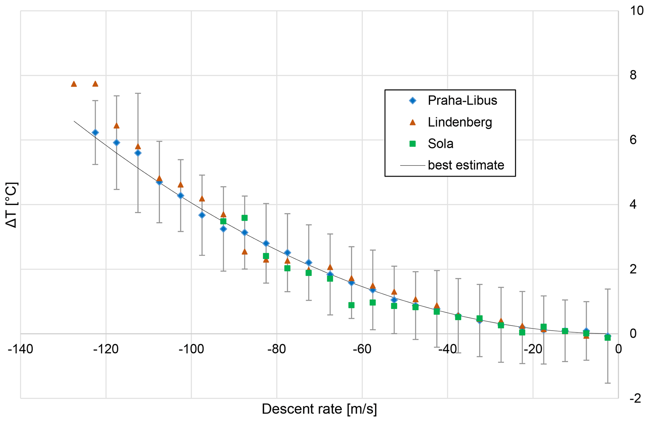
Figure 17 The dependence of temperature differences between ascent and descent on descent rate, showing Praha-Libus, Lindenberg and Sola averaged over different times. For Praha-Libus, the standard deviation and best estimate are shown.

For DR greater than 110 m s⁻¹, the fit is slightly worse, but the sample size is small, with data available from less than 3 % of the examined soundings. When Eq. (2) with $A=\mathrm{4.05}\times {\mathrm{10}}^{-\mathrm{4}}$ is applied as a temperature correction, the root mean square ΔT is lowered from 1.22 to 1.06 ^∘C, indicating that the correction explains 24.4 % of the variance seen.

Calculating the correction as a complete quadratic equation ($\mathrm{\Delta }T=\mathrm{4.39}\times {\mathrm{10}}^{-\mathrm{4}}\times {\mathrm{DR}}^{\mathrm{2}}-\mathrm{3.17}\times {\mathrm{10}}^{-\mathrm{3}}\times \mathrm{DR}+\mathrm{5.40}\times {\mathrm{10}}^{-\mathrm{2}}$) did not significantly improve the result (the explained variance increased by less than 0.01 %).

To find out if the result was affected by lower-tropospheric differences (which are mostly caused by diurnal variation and not friction), the result was recalculated for the sample with all data below 4 km excluded. The results again changed only very slightly: the coefficient was then $A=\mathrm{4.04}\times {\mathrm{10}}^{-\mathrm{4}}$, and the explained variance increased to 25.3 %.

The coefficients were also calculated separately for the data from each time of the launch – the 00:00, 06:00 and 12:00 UTC soundings – and the estimates of coefficient A ranged from $\mathrm{3.9}\times {\mathrm{10}}^{-\mathrm{4}}$ to $\mathrm{4.3}\times {\mathrm{10}}^{-\mathrm{4}}$ (Table 3).

Table 3 Best estimate of the correction coefficient for different times of launch at Praha-Libus.

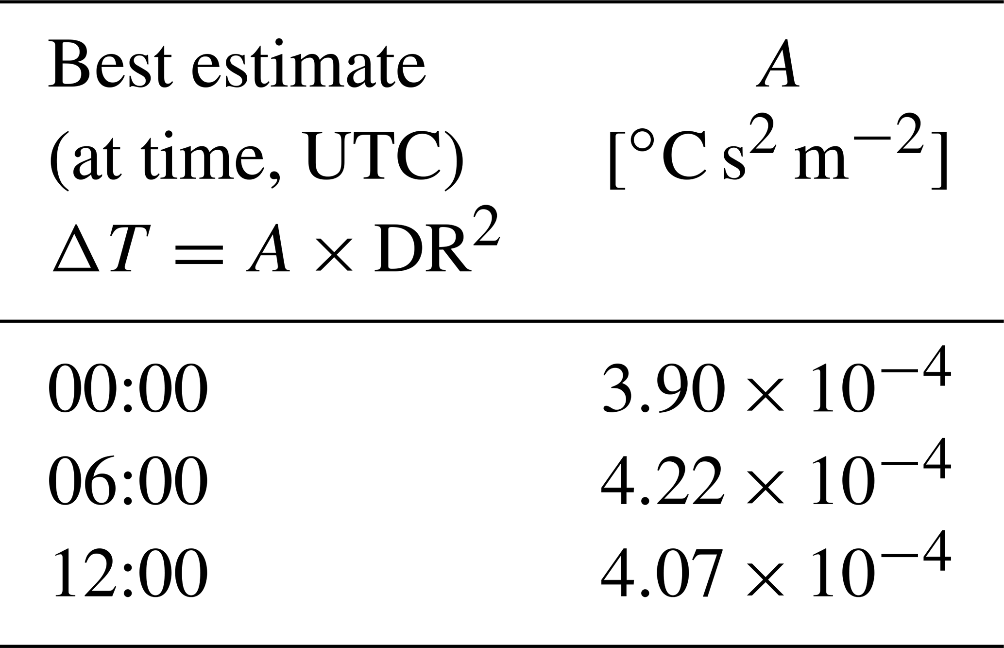
Figure 18 shows the mean and SD of ΔT as a function of height before and after applying the correction. We can see that the bias was almost completely removed, except for the lowest layers, where the bias is expected due to diurnal effects. Another notable result was that the ΔT SD for heights above 20 km was significantly lowered.

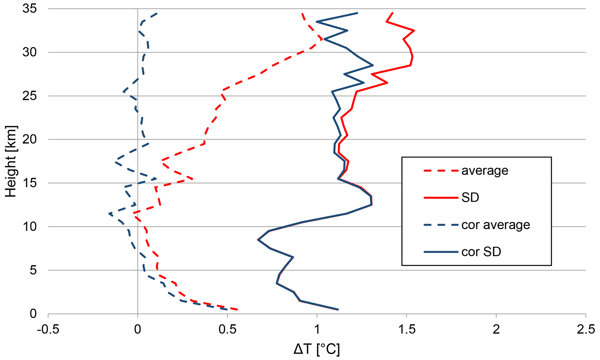
Figure 18 Average ΔT and its standard deviation (SD) before and after friction correction (Praha-Libus).

Investigations were extended to other stations to examine consistency. Information about the type of the data, the data sample and the calculated coefficient is given in Table 4.

Table 4 The coefficient A determined from different samples.

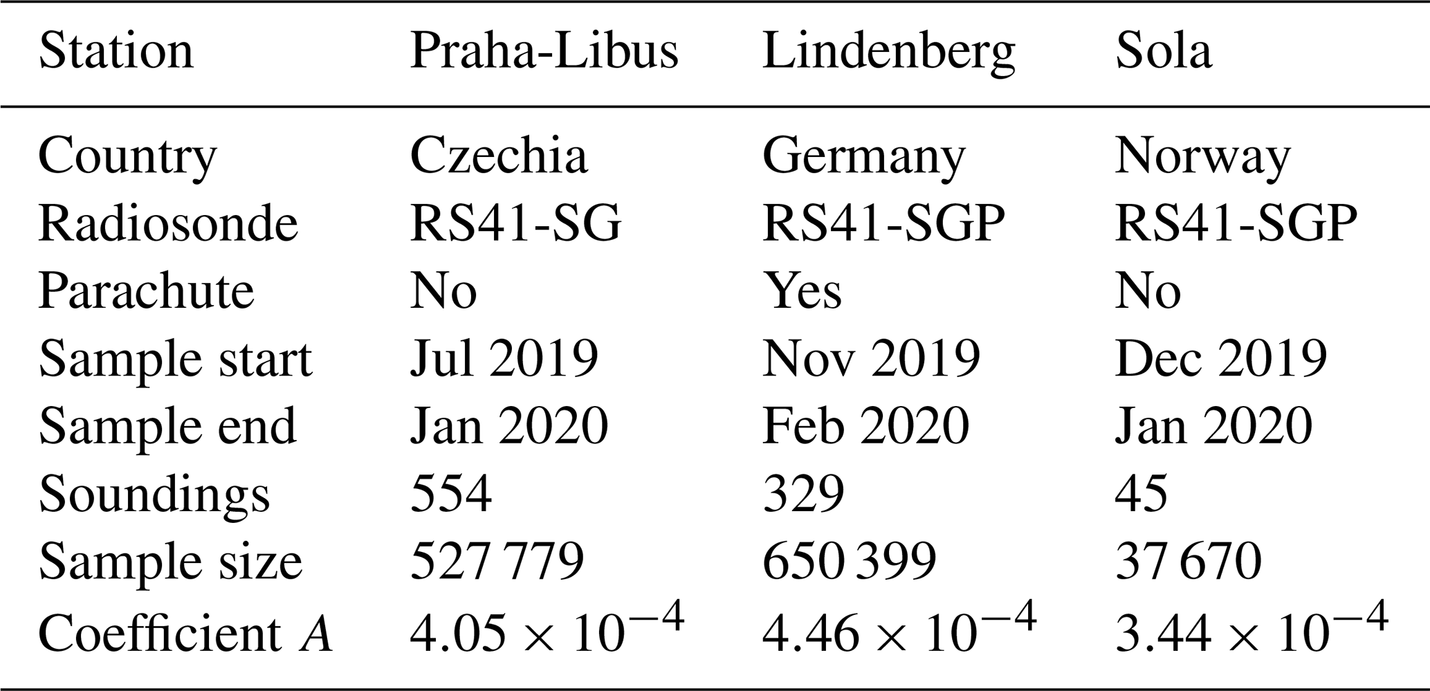
It can be seen from the results in Table 4 that the exact value of the correction coefficient is slightly uncertain. To check with a larger sample, Fig. 19 shows the differences from the ECMWF background for the 20 to 30 hPa layer but with the descent temperatures adjusted using $A=\mathrm{4}\times {\mathrm{10}}^{-\mathrm{4}}$. This does a good job of removing the speed-dependent biases seen in Fig. 14 (the correction also works well at other stratospheric levels). This suggests that it may be sufficient to have the same correction applied with and without a parachute.

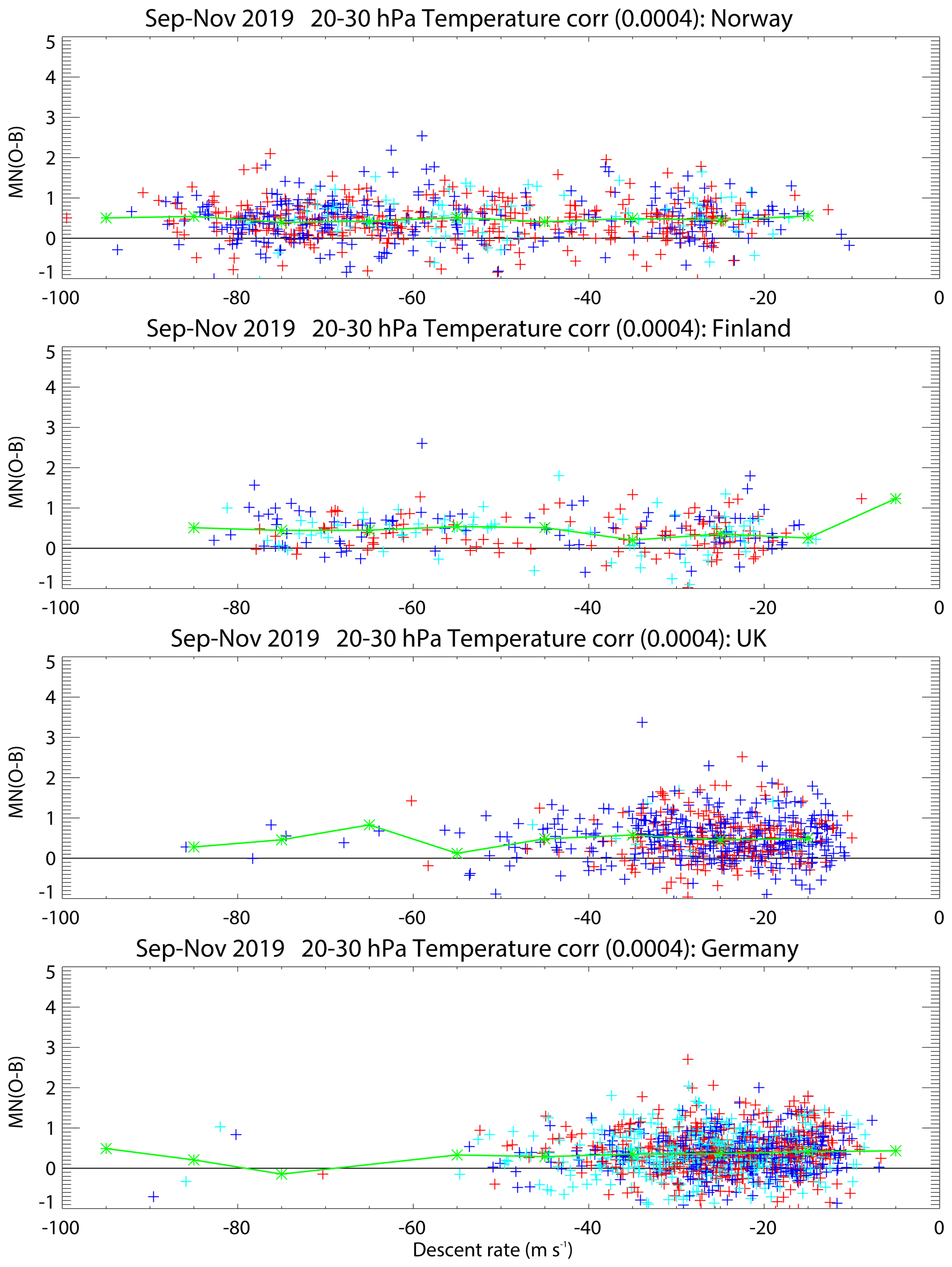
Figure 19 Comparison between the mean fall speed from 20 to 30 hPa and the mean O − B temperature after correction using A=0.0004 (cf. Fig. 14). Green markers show the values averaged over all times of the day in bins of 10 m s⁻¹.

4.2 The indirect effect of heating

Some radiosondes, including the RS41-SGP, measure atmospheric pressure directly, and the geopotential height is calculated using the hydrostatic equation: $dP=-\mathit{\rho }\left(H\right)gdH$, where the density of air ρ depends on pressure, temperature and humidity. The RS41-SG radiosonde measures geometric height using GPS; this is converted to geopotential height, and the pressure is calculated with the hydrostatic equation.

As discussed above, descent at high speeds, mostly in the stratosphere, causes the measured temperature to be too high. This overestimation of temperature leads to an underestimation of air density. For the RS41-SGP, this means that (negative) height increments are smaller than they should be; thus, for a certain pressure level, higher altitudes are reported than they should be. As the height errors accumulate during the descent, the shift of height affects the troposphere levels, where the direct heating impact is negligible. For RS41-SG radiosondes, the effect is similar, resulting in an underestimation of pressure increments, causing a lower pressure for a given height (illustrated in Fig. 20).

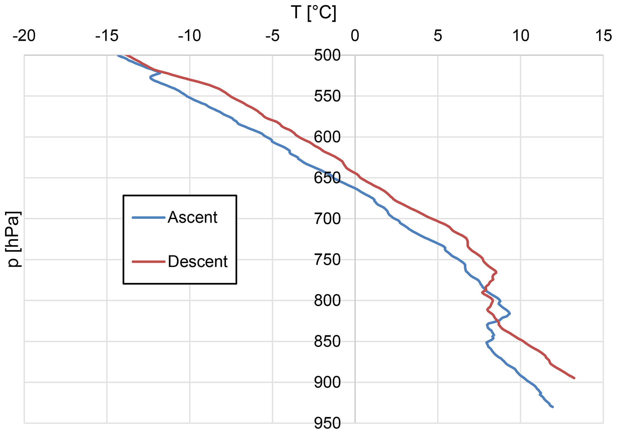
Figure 20 Shift of the tropospheric profile as a function of pressure: profile from 23 September 2019, 12:00 UTC, Praha-Libus.

The shift of the profile is visible only if we use the calculated variable as the vertical coordinate, rather than the directly measured variable. As most applications (including many NWP systems) use pressure as a vertical coordinate, the effect can be seen for RS41-SG radiosondes. It should lead to an increase in SD when comparing variables to the NWP model as well as to an increase in the tropospheric temperature bias due to the temperature gradient in the troposphere (as can be seen in Finnish data compared to ECMWF in Fig. 13).

The effect is clearly visible in Fig. 21. For the Praha-Libus data sample, the ascent and descent levels were matched using both height and pressure respectively. In the stratosphere, the choice of coordinate has little impact on the ΔT statistics (because ΔT comes mainly from direct heating). In the troposphere, the friction is much lower due to the slower DR, and the shift of the profile caused by accumulated pressure errors is responsible for most of the bias for pressure-matched levels. Up to 11 km, there is also visible worsening of the SD for pressure-matched profiles due to this effect.

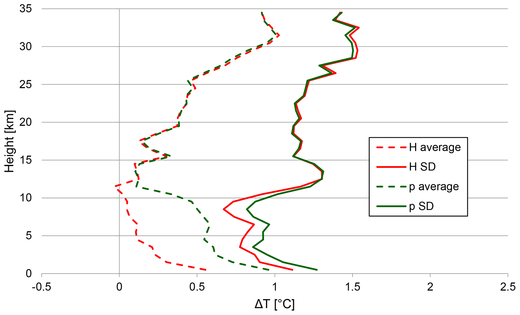
Figure 21 The temperature (T) bias and standard deviation (SD) when ascent and descent levels are matched using height (red) or pressure (green), averaged over 7 months of Praha-Libus profiles.

The improvement in the pressure differences after the application of the temperature correction, Eq. (2), and recalculating pressure using corrected temperature is clearly visible in Fig. 22. The recalculation was made on a data sample from Praha-Libus, and the pressure bias near the surface was decreased by approximately 95 %.

Figure 22 The average pressure difference ($\mathrm{\Delta }p=p_{\mathrm{ascent}}-p_{\mathrm{descent}}$) and its standard deviation (SD) before and after applying temperature correction for friction and pressure recalculation.

Figure 23 shows the bias (dashed) and SD (solid) relative to the ascent for two versions of Praha-Libus temperature descent data (all the data used T_cor according to Eq. 2); data were matched by pressure that was either reported or recalculated using the corrected temperature. The negative effect of accumulated pressure error due to friction (green line) was removed by the pressure correction. The corrected (purple) lines on Fig. 23 are almost identical to the red lines on Fig. 21 using data matched by height. Thus, the pressure errors arising from stratospheric heating of the temperature sensor can largely be removed by using corrected temperatures in the hydrostatic calculations.

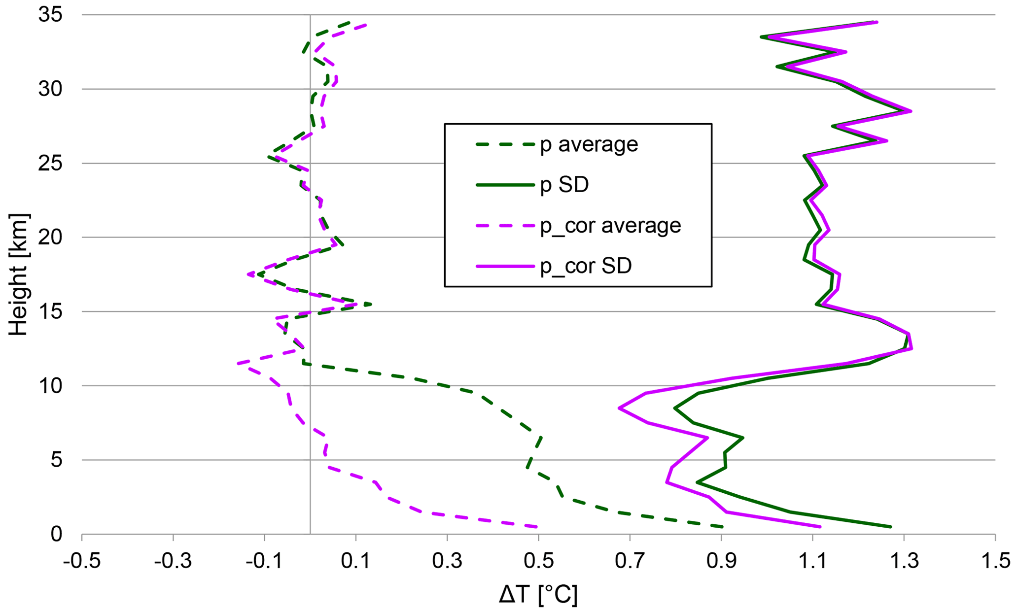
Figure 23 The temperature (T) bias and standard deviation (SD) between ascent and descent matched using either reported pressure (green) or corrected pressure (purple). Accumulated Praha-Libus data were used, and the friction correction was applied to all temperatures.

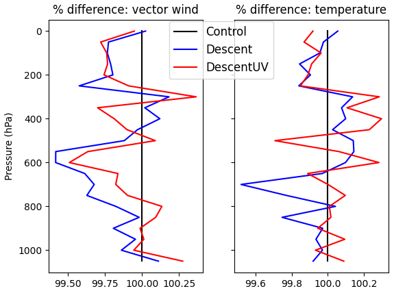
Figure 24 The effect of the assimilation of all descent data (wind, temperature and humidity; blue line) or just descent winds (red line) for the period from 20 January to 20 April 2020. Results are shown for temperature and the vector wind fit of 12 h forecasts to European radiosonde ascents, normalised by the fit of the control forecasts (so values less than 100 % indicate improved forecasts).

5 Assimilation of descent data

Partly prompted by the drop in the number of aircraft data due to the Covid pandemic (Ingleby et al., 2021), a trial was run assimilating European RS41 descent data for 20 January to 28 April 2020. The large-scale impact was very small, as expected, but there were modest improvements in the root mean square (rms) fit of the 12 h forecast to radiosonde ascent data over Europe (Fig. 24 100*rms_test/rms_control is shown). There were improvements over Germany (not shown), and the impact was mixed over Scandinavia. The decision was made to assimilate only the German descent data for the time being; this is the best subset of data, as the instruments have parachutes and pressure sensors, as discussed in Sect. 3. This was implemented operationally on 17 June 2020. Upper-level temperatures were excluded because of the biases. Upper-level winds were used in the trial; however due to concerns about accuracy when the radiosonde is falling fast, all descent data with pressure less than 150 hPa are excluded in the current operational system. Note that, at the upper levels, the ascent and descent are close together in space and time; therefore, one may not want to assimilate both ascent and descent profiles. As discussed in Sect. 4, some of the bias problems would be reduced if height was used as the vertical coordinate rather than pressure; however, this would involve significant work and testing, so there are no plans to do so in the near future.

6 Discussion and conclusions

The most obvious difference between ascent and descent data is that the descent temperatures are higher at upper levels. This has previously been noted for different radiosonde types (by Tiefenau and Gebbeken, 1989, and Venkat Ratnam et al., 2014). Our results suggest that the descent temperatures are too high and that this is closely linked to the descent rate (Fig. 14). In Fig. 17, the dependence on descent rate appears to be quadratic. Vaisala are working on updated processing to address the temperature bias and other issues. There has been considerable discussion on the source of the ascent–descent temperature differences. Whilst we cannot definitively explain the heating mechanism, a plausible hypothesis is the conversion of kinetic energy via frictional heating. Clearly the falling radiosonde (in addition to the balloon remains and parachute if fitted) is slowed by friction, otherwise it would accelerate to much higher speeds during the descent. Future work might include testing radiosonde sensors in a wind tunnel with a flow of 20 m s⁻¹ or more to see if the heating is replicated (care would be needed with the reference temperature). We have not been able to find such tests in the literature. There is a paper by de Podesta et al. (2018) about the effect of sensor diameter on temperature errors, but they were looking at lower flow rates.

Another difference that does not seem to have been reported before is that the descent winds are smoother on average than the ascent winds. In part, this is because ascents are generally more affected by pendulum motion; however, inertial effects and the filtering applied to “remove” pendulum motion also play a role. The smoother descent winds have a closer overall fit to the NWP winds, but we cannot currently say whether the ascent or descent winds are more accurate. Most studies of radiosondes concentrate on the temperatures and humidities, and the winds are somewhat neglected; the use of long strings improves stratospheric temperatures at the expense of increasing the pendulum motions. For aircraft, the winds have more than twice the impact of the temperatures on the quality of short-range forecasts (Ingleby et al., 2021), and forecast sensitivity diagnostics suggest that the same is true of radiosondes (Pauley and Ingleby, 2021), partly because satellite instruments primarily provide temperature and humidity data. Experience shows that GPS winds are generally good quality and biases do not seem to be a problem. GPS can provide high-vertical-resolution winds, but this makes pendulum motion more obvious; hence, the avoidance or removal of pendulum motion deserves more attention. One technique to obtain accurate wind profile data is the Jimsphere – a balloon with roughness elements used without a separate instrument package. Sako and Waltersheid (2016) discuss empirical filtering of wind profiles from radiosondes and Jimsphere balloons. Dropsonde wind profiles suffer much less from pendulum motion than radiosonde ascent winds (Wang et al., 2008) and probably less than radiosonde descent winds. The two balloon ascents of Kräuchi et al. (2016) largely eliminate pendulum motion but need more evaluation.

Some aspects of the descent data can be improved by estimating and removing heating effects due to high fall rates (on the temperature as well as on the pressure for radiosondes without a pressure sensor). The descent characteristics are more variable than ascent rates in that, for balloons with parachutes, how the parachute deploys can affect the amplitude of the pendulum motion and the descent speed. It is also likely that there can be improvements in the filtering of pendulum motion. Vaisala are working on these aspects but are not yet ready to give a timescale for changes. In principle, users could apply bias corrections, but improving the winds is difficult if they have already been filtered. On the whole, it is simplest to stick to the current practice of manufacturers providing best-estimate profiles, but more details of the processing would be welcome, and this area should be kept under review. On a similar note, there is the question of whether there should be a GRUAN descent product for the RS41 – more work on the uncertainties would be needed for this. There is also the wider question of how much the lessons learnt from the RS41 descent are applicable to other radiosondes, such as the Meteomodem M10. There is some evidence that pressure sensor accuracy is worse whilst falling fast, but more work on this is needed. However the fall speed should have very little effect on the accuracy of GPS-derived positions, as the GPS satellites are moving much faster anyway.

There is evidence (Figure 13) that use of parachutes and/or pressure sensors somewhat improves the descent data (the benefits of parachutes or pressure sensors will decrease with improved processing/bias correction). There is also the possibility of installing extra receivers to obtain more descent data from the lower troposphere (this has been demonstrated in Corsica, Olivier Peyrat, personal communication, 2020). Whether the extra costs are worthwhile would need to be assessed. We note that the impact of extra radiosonde profiles over well-observed Europe will be less than the impact of extra profiles near remote islands or ships. In May 2021, descent data were received from several European ships in the North Atlantic and from a station in Antarctica. The ECMWF and DWD have started operational assimilation of a subset of descent profiles – excluding the stratospheric segment with higher average fall rates (it would be better to exclude data based on the actual descent rate, but this would require more work). The US Navy global model is assimilating all available descent profiles (Patricia Pauley, personal communication, 2021), but we are not aware of other NWP systems using them yet. NWP systems generally use pressure as the vertical coordinate for radiosonde data, although there would arguably be advantages in using height instead. There has been much more use of NWP model fields in this investigation than is traditional for the development and validation of in situ observations (but is routine now for new satellites – Newman et al., 2020). This means that a much larger sample can be examined. Note that traditional radiosonde intercomparisons (e.g. Nash et al., 2011) cannot be used to assess descent data because the multi-radiosonde rig used has various implications for the descent, including possible entanglement. Descent data should be used with caution, particularly sections with high descent rates; however, different users have different tolerances, and we expect that improved processing will increase the proportion of usable data.

Appendix A: Comparison with aircraft temperatures

For cruise-level aircraft (typical speed of about 250 m s⁻¹), the measured temperature, known as the total air temperature (TAT), can be more than 20 K higher than the static air temperature (SAT). The link between TAT and SAT (Wendisch and Brenguier, 2013) can be expressed as follows:

$$\begin{array}{}\text{(A1)}& \mathrm{SAT}={\displaystyle \frac{\mathrm{TAT}}{\mathrm{1}+\frac{r(\mathit{\gamma }-\mathrm{1})}{\mathrm{2}}\cdot M^{\mathrm{2}}}},\end{array}$$

where r is the recovery factor of the sensor, γ is the adiabatic index and M is the Mach number.

From Eq. (A1), we can get the difference $\mathrm{TAT}-\mathrm{SAT}=\mathrm{SAT}\cdot \frac{r(\mathit{\gamma }-\mathrm{1})}{\mathrm{2}}\cdot M^{\mathrm{2}}$.

If we use the Mach number ($M=\frac{v}{a}$, where v is the airspeed of the object (aircraft or radiosonde), and a is the speed of sound, given by $a=\sqrt{\mathit{\gamma }\cdot (C_{\mathrm{p}}-C_{\mathrm{v}})\cdot \mathrm{SAT}}$, where C_p and C_v are heat capacity constants for constant pressure and volume respectively), we can get

$$\begin{array}{}\text{(A2)}& \mathrm{TAT}-\mathrm{SAT}={\displaystyle \frac{r(\mathit{\gamma }-\mathrm{1})}{\mathrm{2}}}\cdot {\displaystyle \frac{v^{\mathrm{2}}}{\mathit{\gamma }\cdot \left(C_{\mathrm{p}}-C_{\mathrm{v}}\right)}}.\end{array}$$

Applying $\mathit{\gamma }=\frac{C_{\mathrm{p}}}{C_{\mathrm{v}}}$ to Eq. (A2), the difference between the measured and real temperature is

$$\begin{array}{}\text{(A3)}& \mathrm{TAT}-\mathrm{SAT}={\displaystyle \frac{v^{\mathrm{2}}}{\mathrm{2}{C}_{\mathrm{p}}}}r.\end{array}$$

According to the Wikipedia entry on total air temperature (https://en.wikipedia.org/wiki/Total_air_temperature, last access: 5 January 2022), the typical recovery factor for platinum wire (which is used for radiosondes) is 0.75–0.9. Even if we are not sure about the exact physical process of kinetic energy transfer to internal heat in case of radiosondes, we might expect similar behaviour (a quadratic dependency on descent rate but independent of height, temperature and air density). When we apply Eq. (A3) to descending radiosondes, where v is the descent rate (DR) of the radiosonde, with the range 0.75–0.9 for r we get

$$\begin{array}{}\text{(A4)}& \begin{array}{rl}\mathrm{TAT}-\mathrm{SAT}=& A\times {\mathrm{10}}^{-\mathrm{4}}\times {\mathrm{DR}}^{\mathrm{2}},\mathrm{with}A\mathrm{in}\mathrm{the}\mathrm{range}\mathrm{from}\\ & \mathrm{3.70}\mathrm{to}\mathrm{4.47}.\end{array}\end{array}$$

However, the similar coefficients for aircraft and descent radiosondes may come from different conversion mechanisms.