Emissivity retrievals with FORUM's end-to-end simulator: challenges and recommendations

Spectral emissivity is a key property of the Earth's surface, of which only very few measurements exist so far in the far-infrared (FIR) spectral region, even though recent work has shown that the FIR is important for accurate modelling of the global climate. The European Space Agency's 9th Earth Explorer, FORUM (Far-infrared Outgoing Radiation Understanding and Monitoring) will provide the first global spectrally resolved measurements of the Earth's top-of-the-atmosphere (TOA) spectrum in the FIR. In clear-sky conditions with low water vapour content, these measurements will provide a unique opportunity to retrieve spectrally resolved FIR surface emissivity. In preparation for the FORUM mission with an expected launch in 2027, this study takes the first steps towards the development of an operational emissivity retrieval for FORUM by investigating the sensitivity of the emissivity product of a full spectrum optimal estimation retrieval method to different physical and operational parameters. The tool used for the sensitivity tests is the FORUM mission's end-to-end simulator. These tests show that the spectral emissivity of most surface types can be retrieved for dry scenes in the 350–600 cm⁻¹ region, with an absolute uncertainty ranging from 0.005 to 0.01. In addition, the quality of the retrieval is quantified with respect to the precipitable water vapour content of the scene, and the uncertainty caused by the correlation of emissivity with surface temperature is investigated. Based on these investigations, a road map is recommended for the development of the operational emissivity product.

1 Introduction

The European Space Agency's 9th Earth Explorer, FORUM (Far-infrared Outgoing Radiation Understanding and Monitoring; Palchetti et al., 2020) is scheduled to launch in 2027. FORUM will provide spectrally resolved measurements of the Earth's top-of-the-atmosphere (TOA) outgoing radiation from 100 to 1600 cm⁻¹, with the goal of filling the observational gap in the far-infrared (FIR; defined here as below 667 cm⁻¹). Even though simulations suggest that around 50 % of the outgoing longwave radiation (OLR) to space is in the FIR in the global mean, due to technical reasons it has never been observed from satellite, spectrally resolved, in its entirety. FORUM's novel measurements will be provided by the mission's core instrument, a nadir-viewing Fourier transform spectrometer (FTS), which will measure the Earth's upwelling spectral radiance. While the primary goal of FORUM is to provide these calibrated spectral radiances, its further aim is to exploit instantaneous radiance observations to retrieve atmospheric and surface properties (Level 2 products).

FORUM clear-sky radiances will be used to retrieve temperature and water vapour profiles, as well as FIR surface emissivity and surface temperature. This work focuses on the retrieval of surface emissivity, which is the material property determining how much thermal radiation a surface emits at a given temperature. For a surface (or skin) temperature T_s, it is defined as the ratio of surface emission to the blackbody emission at T_s. Emissivity is not constant across the spectrum, and the emissivities of different surfaces exhibit distinct spectral variation. The possibility to retrieve spectrally resolved FIR emissivity with FORUM is particularly exciting given its potential influence on the surface and top-of-atmosphere energy budget (Feldman et al., 2014; Kuo et al., 2018).

Surface emissivity across the globe is routinely retrieved in the mid-infrared (MIR) from satellite observations (Susskind et al., 2014; Capelle et al., 2012; Masiello and Serio, 2013; Wan, 2014; Wang et al., 2005). These are complemented by laboratory measurement datasets such as the Advanced Spaceborne Thermal Emission and Reflection Radiometer (ASTER) spectral library, which includes more than 2300 different spectral emissivities down to 650 cm⁻¹ (Baldridge et al., 2009). However, in the FIR, no global retrievals of surface emissivity are available due to the absence of spectrally resolved TOA radiance observations, and there is also a lack of laboratory measurements. Bellisario et al. (2017) and Murray et al. (2020) were the first to retrieve FIR snow emissivities from aircraft measurements (during the CIRCCREX/COSMICS projects over Greenland), confirming the feasibility of retrieving FIR surface emissivity from OLR spectral measurements. However, in these studies, no existing theoretical snow/ice model fit the retrieved emissivity values in the MIR and FIR simultaneously, indicating that further testing of the theoretical models using global emissivity retrievals is vital to extend surface emissivity datasets into the FIR. While other planned FIR measurements, such as the Polar Radiant Energy in the Far Infrared Experiment (PREFIRE; L’Ecuyer et al., 2021) and ground-based measurements of snow emissivity (see Palchetti et al., 2021), will contribute to our understanding of FIR emissivity, only FORUM will be able to provide such global retrievals.

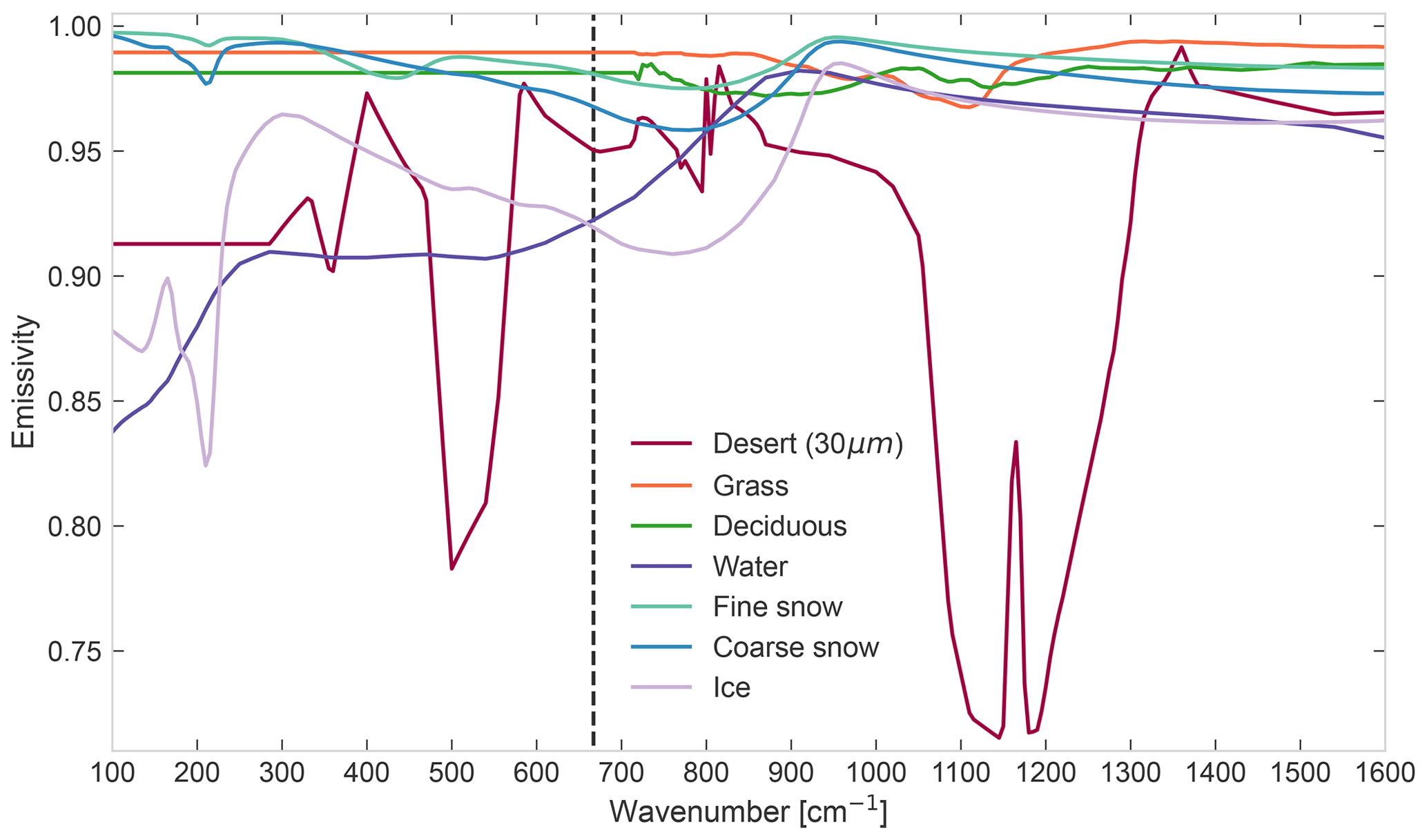
Figure 1 Spectral surface emissivity between 100 and 1600 cm⁻¹ for 7 out of the 11 surface types in Huang et al. (2016). The desert subtype is r_e=30 µm, as used in the FEES. The far-infrared is defined in this work to the left of the dashed line.

The potential value of knowing the spectral variation in surface emissivity in the FIR is significant. In recent years, there has been increasing focus on the inadequate representation of surface emissivity in global climate models (GCMs), which almost all assume blackbody or greybody emissivity (Huang et al., 2018). To test the validity of this assumption in the FIR, Feldman et al. (2014) incorporated spectrally varying FIR emissivity into the Community Earth System Model I (CESM I) and showed significant changes in its predictions after 25 years. At high latitudes, as much as a 2 K change in surface temperature and 10 Wm⁻² in the outgoing longwave radiation occurred. The authors also identified a possible feedback mechanism associated with FIR emissivity, namely that in the FIR the emissivity of snow can be substantially higher than that of water (while in the MIR the difference is less significant; see Fig. 1). This means that, as sea ice melts in a warming climate, it exposes a potentially less emissive water surface, exacerbating the warming. Further work with the CESM has confirmed that this feedback is present, if small, and has shown that the inclusion of realistic surface emissivity in fact significantly reduces the persistent cold pole bias of climate models (Kuo et al., 2018; Huang et al., 2018). Critically, by comparing the assumption of ice vs. snow emissivity in the models, it was shown that the size and sign of the feedback depends on the properties of the surface (Huang et al., 2018).

While work has already been done to analyse the performance of the geophysical products (including emissivity) expected from FORUM clear-sky measurements (e.g. Ridolfi et al., 2020; Sgheri et al., 2022), in this study, we focus on spectral surface emissivity and investigate its retrieval using the FORUM mission's end-to-end simulator (FEES) described in Sgheri et al. (2022). In addition to investigating the retrieval parameters, this work focuses on the influence of atmospheric water vapour, as it is one of the most important factors influencing the transmission in the FIR (Harries et al., 2008) due to the dominance of the water vapour rotational band on atmospheric absorption in this region (see Sect. 5).

The paper is structured as follows: Sect. 2 describes the FEES and Sect. 3 the experimental set-up. In Sect. 4, the general FEES retrieval result is introduced, together with the different quantifiers used for its analysis. The parameters are then investigated in the following two steps:

• In Sect. 5, the water vapour profile in the forward model is modified to compare emissivity retrieval quality against scene humidity.

• In Sect. 6, the parameters of the retrieval algorithm associated with surface temperature and emissivity are investigated, i.e. the retrieval a priori, the a priori uncertainty and the initial guess.

Finally, Sect. 7 summarizes the results, focusing on the main challenges and on the recommendations this study has for further development towards an operational emissivity retrieval for FORUM. The three appendixes provide more detail on the emissivity–surface temperature parameter space (Appendix A), the choice of the emissivity a priori uncertainty (Appendix B) and the spectral dependence of the emissivity–surface temperature correlation (Appendix C).

As this work is meant to provide the first steps towards the development of an operational emissivity retrieval for FORUM, the focus is placed on investigating the effect of various factors on the retrieval of a range of typical scenes. The aim of an operational retrieval is to provide the users with a retrieved product that is transparent and accessible, together with a realistic uncertainty estimate. Thus, the focus of this work is not on extreme cases or on optimizing the retrieval for specific scenes but rather on highlighting general features which need to be investigated in the years up to the expected launch in 2027.

2 The FORUM end-to-end simulator and the optimal estimation method

The FORUM mission's end-to-end simulator (FEES) constitutes a chain of modules which simulate the elements relevant to the mission performance. A full description of the FEES can be found in Sgheri et al. (2022), together with a discussion of the geophysical products not shown in this work. Our study uses the following five modules of the simulator: the Geometry Module (GM), the Scene Generator Module (SGM), the FORUM Sounding Instrument (FSI) module, the FORUM Embedded Imager (FEI) module and the Level 2 Module (L2M). For the purpose of this work, the first four modules are run in the default chain (see Sgheri et al., 2022) to generate synthetic FORUM observations for various geographic scenes in clear-sky conditions. The L2M uses these synthetic observations to retrieve the geophysical properties of the scene, and in this work, this retrieval algorithm is tested with a focus on the retrieved spectral surface emissivity.

The L2M retrieves the atmospheric state from the synthetic FORUM measurements using the optimal estimation (OE) method, which deals with the ill-posed nature of the inverse problem using an a priori regularization (Rodgers, 1976, 2000). Starting from an initial guess of the n-dimensional atmospheric state vector x, the algorithm arrives at a best estimate $\widehat{\mathit{x}}$ by minimizing the cost function ξ² as follows:

$$\begin{array}{}\text{(1)}& \begin{array}{rl}{\mathit{\xi }}^{\mathrm{2}}\left(\mathit{x}\right)& =(\mathit{y}-f(\mathit{x}\left){)}^T{\mathbf{S}}_y^{-\mathrm{1}}\right(\mathit{y}-f\left(\mathit{x}\right))\\ & +\left(({\mathit{x}}_{\text{a}}-\mathit{x}{)}^T{\mathbf{S}}_{\text{a}}^{-\mathrm{1}}({\mathit{x}}_{\text{a}}-\mathit{x})\right).\end{array}\end{array}$$

The first term on the right-hand side is the χ² of the forward model, which is in essence the difference between the m-dimensional observation vector y and the forward model f(x) calculated from the atmospheric state vector x, where the covariance matrix S_y represents the uncertainty on the observations. The second term is the regularization term, which takes into account the difference of the state vector x from an a priori (model) atmospheric state x_a with uncertainty S_a. For more details on the forward model and minimization technique, see Sgheri et al. (2022, 2020), and for the parameters and assumptions used in this work, see Sect. 3.

To understand the parameters influencing the quality of the retrieved emissivity, it is useful to keep in mind the role emissivity plays in the forward model, which is in the simulation of the atmospheric radiative transfer. For nadir-looking observations, the clear-sky TOA spectral radiance S_toa,σ at wavenumber σ can be written as follows:

$$\begin{array}{}\text{(2)}& S_{\text{toa},\mathit{\sigma }}=S_{\text{surf},\mathit{\sigma }}{\mathcal{T}}_{\mathit{\sigma }}\left(z_{\mathrm{1}}\right)+\underset{z_{\mathrm{0}}}{\overset{z_{\mathrm{1}}}{\int }}{B}_{\mathit{\sigma }}\left(T\right(z\left)\right){\displaystyle \frac{\partial {\mathcal{T}}_{\mathit{\sigma }}\left(z\right))}{\partial z}}\text{d}z,\end{array}$$

where B(T) is the Planck function, T(z) is the atmospheric temperature profile, 𝒯(z) is the transmittance between the surface and height z, and the integral is over the height z from the surface z₀ to the TOA z₁. 𝒯(z₁) is the transmittance from the surface to the TOA. The emissivity contributes to the surface part of the radiance as follows:

$$\begin{array}{}\text{(3)}& S_{\text{surf},\mathit{\sigma }}=L_{\text{d},\mathit{\sigma }}(\mathrm{1}-{\mathit{ϵ}}_{\mathit{\sigma }})+{\mathit{ϵ}}_{\mathit{\sigma }}{B}_{\mathit{\sigma }}\left(T_{\text{s}}\right).\end{array}$$

Here L_d,σ is the downwelling radiance at the surface, T_s is the surface (or skin) temperature, and ϵ_σ is the emissivity of the surface at wavenumber σ. Following the reasoning from Bellisario et al. (2017), in this work the emissivity is always assumed to have no directional dependence.

3 Experimental set-up

All the results presented in this work are the products of FEES runs. A complete description of this simulator and its modules can be found in Sgheri et al. (2022), and unless otherwise stated, the same parameters and settings are used as described in that work for homogeneous clear-sky cases.

3.1 FEES modules

Only the first five modules of the FEES are used in this work. The Scene Generator Module (SGM), which uses geographic coordinates provided by a Geometry Module, computes high-resolution TOA spectral radiances in clear sky conditions using the radiative transfer model LBLRTM version 12.8 (Clough et al., 2005) and auxiliary databases prepared for the FEES. For a detailed description of the auxiliary datasets, see Sgheri et al. (2022), but for reference, note that the water vapour and temperature profiles and the surface temperature are taken from ERA5 reanalysis data (Hersbach et al., 2020). In this work, all scenes used are from 15 January 2018 at 12:00:00 UTC for consistency, and they are identified using their geographic coordinates (see Table 1). The emissivity dataset used by the SGM is based on the geolocated dataset of spectral emissivity by Huang et al. (2016) and uses the 11 surface types defined by Huang et al. (2016) (out of the multiple desert subtypes, the r_e=30 µm subtype is used). Each scene is generated using the surface type out of these 11 that best match the January value in the geolocated dataset for the given coordinates. A total of 7 of these 11 surface types can be seen in Fig. 1.

Table 1 Atmospheric and surface data for the various scenes used in this study. All data are for 15 January 2018 at 12:00:00 UTC. Surface temperatures, surface heights, water vapour profiles and temperature profiles are from ERA5 reanalysis data. Surface types are fitted to the Huang et al. (2016) dataset, as detailed in the text. Note: pwv stands for precipitable water vapour, and T₀−T_s is the difference between the lowest point of the temperature profile and the surface temperature.

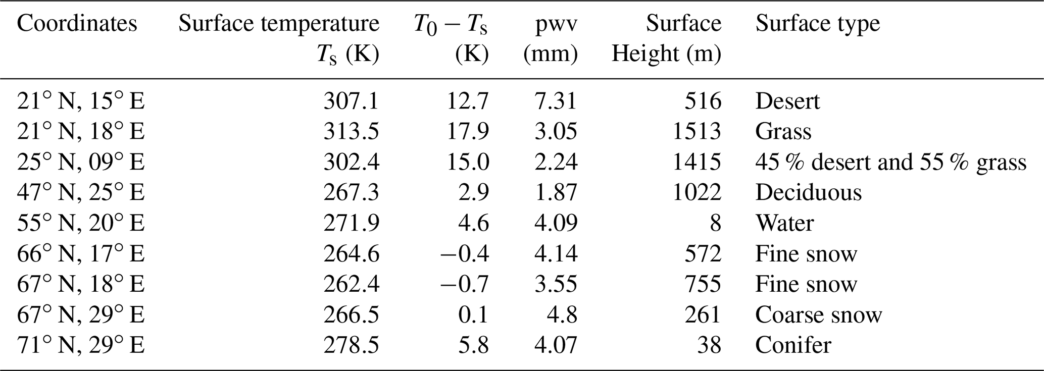
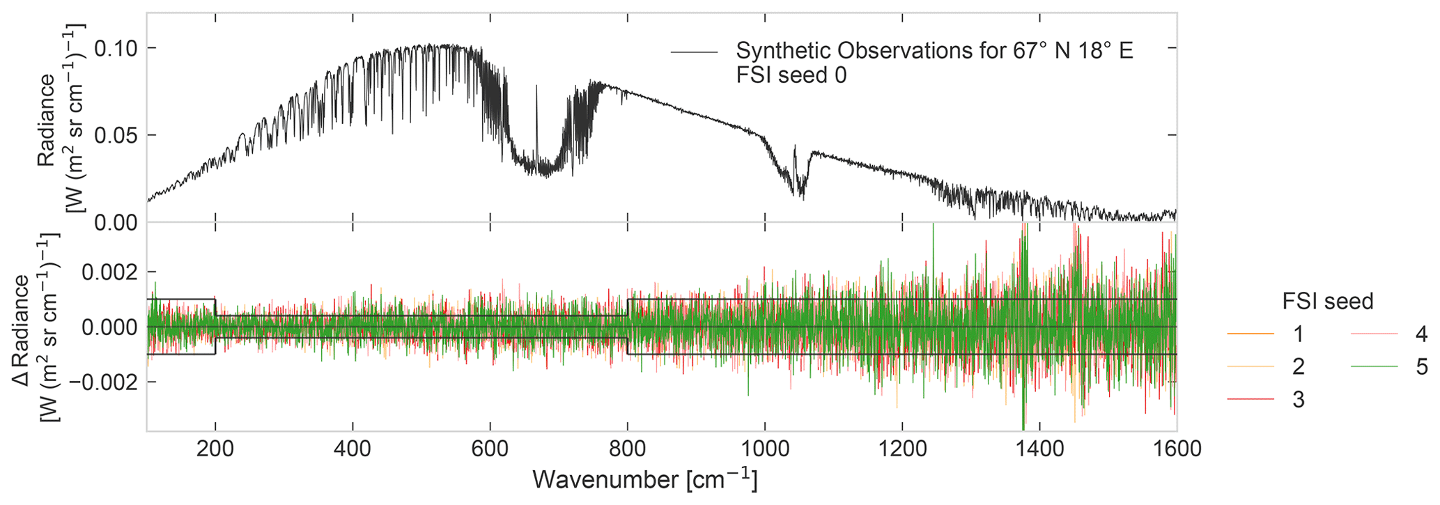
Figure 2 Panel (a) shows an example of synthetic observations generated by the first four modules of the FEES for the scene at 67^∘ N, 18^∘ E on 15 January 2018 at 12:00 UTC. Panel (b) shows the difference in radiance between spectra generated with the FORUM Sounding Instrument (FSI) random noise seeds from 1–8 and the spectrum generated with seed 0 (shown in panel a). The FORUM goal noise equivalent spectral radiance (NESR) is shown as the black lines in panel (b).

The third and fourth modules of the FEES simulate the observing system. The only change made to these modules is to vary a so-called seed used to generate the random noise associated with the FORUM Sounding Instrument (FSI). The synthetic observations thus generated and the variation in random noise is illustrated in Fig. 2.

The final module used is the L2M, which has been described in more detail above in Sect. 2. This is the module used to test emissivity retrieval properties and in which the major modifications were made.

3.2 The baseline retrieval parameters

In this work, the retrieved atmospheric state vector x constitutes the atmospheric water vapour profile, the temperature profile, the spectral surface emissivity and the surface temperature. For the purpose of this study, we define a baseline/default retrieval case, which is used as the basis for all modifications and tests. Unless otherwise stated, all parameters are the standard parameters for clear-sky retrievals in Sgheri et al. (2022). Only two parameters differ between the baseline retrieval in this study and the standard of Sgheri et al. (2022). For the emissivity a priori, this work uses a flat a priori value instead of a perturbed climatological one and a 0.1 uncertainty instead of 0.05 (see Sect. 3.3 and Appendix B for a justification of these choices).

For comparison with later modifications, some of these baseline parameters are listed as follows:

• Emissivity initial guess, which is constant and equal to 1

• Emissivity a priori, which is constant and equal to 1

• Emissivity a priori uncertainty matrix, which is defined using uncertainty Δϵ=0.1 and correlation length (CL) of 50 cm⁻¹ (see Appendix B for an explanation of these terms and a justification of the choice of uncertainty matrix)

• Emissivity retrieval grid, which is an evenly spaced 5 cm⁻¹ grid for the full FORUM spectral range

• Surface temperature initial guess, which is the climatological value from ERA5 monthly averages (different from the daily value used for the SGM)

• Surface temperature a priori, which is a random perturbation of the true value with a 2 K standard deviation (the perturbation is the same for the same geographical scene)

• Surface temperature a priori uncertainty, which is 2 K.

In the baseline retrieval, the same instrumental noise is used for all cases (i.e. the seed used to generate the instrumental random noise is kept the same at a value of 0; see Fig. 2).

To test the retrieval of surface emissivity in the FIR, we choose to use geographic scenes with low precipitable water vapour (pwv), which is defined as the depth of water produced if all water in the atmospheric column precipitated as rain. For reference, the full list of scenes used in the tests shown in this work can be found in Table 1, together with some of their relevant atmospheric and surface properties.

3.3 The emissivity a priori and deviation from classical optimal estimation

In the classical optimal estimation method from Rodgers (2000), the solution represents the estimate of maximum a posteriori probability. In the remote sensing community, x_a is usually an a priori climatology, and so S_a typically represents the natural variability in these climatologies. However, the formalism of the method can be used without giving a probabilistic interpretation to x_a and S_a and simply tuning them to best regularize the retrieval (von Clarmann et al., 2020). For example, the smaller the uncertainties in S_a are, the closer the solution will be on average to x_a; this can be thought of as giving the retrieval more or less freedom to converge to the true state.

In this work, we deviate from the classical OE method and do not use climatological datasets for the emissivity part of the a priori vector (climatologies are still used for the rest of x_a). Instead, a constant emissivity a priori is chosen in combination with a larger uncertainty. This is done to ensure consistency across cases and allow for easier comparison of different retrieval setups. To cover the range of possible theoretical emissivity model values in the considered spectral region, the emissivity submatrix of S_a is chosen to ensure that the emissivity retrieval has the freedom to converge to any physical value (between 0.7 and 1), provided there is enough sensitivity in the measurements. Therefore, the choice of a constant a priori value is rather arbitrary, and the baseline value is taken to be 1 for simplicity. The chosen parameters defining the emissivity submatrix of S_a are an uncertainty Δϵ=0.1 and correlation length (CL) of 50 cm⁻¹ (see Appendix B for an analysis of these).

Future steps in the development of the FORUM operational retrieval can improve on this approach by the use of scene classification and by developing FIR emissivity climatologies for these scenes, as is already implemented in the MIR for retrievals of emissivity from MODIS (Moderate Resolution Imaging Spectroradiometer) observations (Borbas et al., 2018; Feltz et al., 2018; Loveless et al., 2020).

4 The emissivity product, its quantifiers and water vapour

The retrieval process can only give information on a retrieved quantity where the forward model $f\left(\widehat{\mathit{x}}\right)$ is sensitive to this quantity and returns the a priori where there is no sensitivity. For retrievals of surface emissivity from TOA spectral measurements, this is determined by the atmospheric transmission. For high water vapour content, the TOA is opaque to the surface in the FIR but becomes more transparent as the atmosphere gets drier. The distinct characteristic of atmospheric transmission in the FIR is that, as the pwv decreases, transmittance does not increase uniformly but in so-called microwindows, which become deeper as pwv decreases. To illustrate the typical pattern of this sensitivity in the FIR, four different quantifiers are defined in this section, and their behaviour for varying water vapour content is analysed.

4.1 The quantifiers

A total of four different quantifiers are described in the following section to illustrate retrieval quality. These are shown together with the TOA transmittance in Fig. 3 for the baseline retrieval of the scene at 67^∘ N, 18^∘ E.

Figure 3 The retrieved emissivity and four quantifiers used to assess the retrieval quality. The retrieved scene is of fine snow emissivity at 67^∘ N, 18^∘ E on 15 January 2018 12:00 UTC, with default parameters, as outlined in Sect. 3. Panel (a) shows the retrieved emissivity with 1σ retrieval uncertainty error bars in orange, the true fine snow emissivity from Huang et al. (2016) in black and the a priori emissivity in grey. Panel (b) shows the information quantifier (IQ) for this retrieval, as defined in Eq. (5), with the orange bars showing the spectral regions where IQ is larger than 1. Panel (c) shows the diagonal elements of the spectral-resolution emissivity Jacobian of the radiative transfer part of the retrieval forward model at convergence, as defined in Eq. (6). The main absorbers in the respective spectral regions are labelled. In panel (d), the rows of the emissivity submatrix of the averaging kernel (defined in Eq. 7) are plotted with light lines, and the diagonal is plotted with a dark line. Panel (e) shows the top-of-the-atmosphere (TOA) transmittance of the true scene used for synthetic observations.

Figure 3a shows the baseline retrieved emissivity, which is the emissivity part of the best estimate atmospheric state vector $\widehat{\mathit{x}}$ introduced in Sect. 2. Note that the emissivity is retrieved on a 5 cm⁻¹ spectral grid, which is much coarser than the ∼0.4 cm⁻¹ resolution of the synthetic observations, and thus, the emissivity ϵ_σ used in the atmospheric radiative transfer calculations of the forward model (Eq. 3) is in fact a linear interpolation of the emissivity elements of the retrieval vector $\widehat{\mathit{x}}$.

The first quantifier is the retrieval uncertainty, shown as the error bars in Fig. 3a. These are derived from the retrieval uncertainty covariance matrix S_x, defined as in Rodgers (2000), as follows:

$$\begin{array}{}\text{(4)}& {\mathbf{S}}_x={\left({\mathbf{K}}^T{\mathbf{S}}_y^{-\mathrm{1}}\mathbf{K}+{\mathbf{S}}_{\text{a}}^{-\mathrm{1}}\right)}^{-\mathrm{1}},\end{array}$$

where S_y and S_a are as in Eq. (1), and K is the Jacobian of the full forward model at convergence with respect to the retrieval vector. The retrieval standard deviation σ_x is the square root of the diagonal of S_x. σ_x is called the retrieval uncertainty in this work, while the systematic uncertainty is defined as the true value minus the retrieved value.

The second quantifier shown in Fig. 3b makes further use of the information contained in σ_x, in particular that, in regions where there is no sensitivity, the retrieval vector will equal the a priori, and the σ_x will equal the a priori uncertainty σ_a. Recognizing this, Dinelli et al. (2009) defined the information quantifier (IQ) as follows:

$$\begin{array}{}\text{(5)}& \text{IQ}=-{\displaystyle \frac{\mathrm{1}}{\mathrm{2}}}{\log }_{\mathrm{2}}\left({\displaystyle \frac{{\mathit{\sigma }}_x}{{\mathit{\sigma }}_{\text{a}}}}\right),\end{array}$$

where σ_x is as above, and σ_a is the square root of the diagonal of the retrieval a priori covariance matrix S_a. The IQ thus tends to 0 in regions with low sensitivity as σ_x approaches σ_a. Note that, while the IQ can be defined for the full retrieval vector, in this work it is only used for the retrieved emissivity.

The third quantifier is the Jacobian of the TOA radiances with respect to emissivity. While Eq. (4) uses the Jacobian K with respect to the full forward model, to directly quantify the emissivity retrieval quality, a different Jacobian J is used, which is calculated with respect to the radiative transfer simulation at convergence as follows:

$$\begin{array}{}\text{(6)}& J_{ij}={\displaystyle \frac{\partial F_{\text{toa},{\mathit{\sigma }}_i}}{\partial {\mathit{ϵ}}_{{\mathit{\sigma }}_j}}},\end{array}$$

where ${\mathit{ϵ}}_{{\mathit{\sigma }}_j}$ are the emissivity values used in the radiative transfer calculations of LBLRTM, and $F_{\text{toa},{\mathit{\sigma }}_i}$ are the resulting TOA radiances at wavenumbers σ_i and σ_j (see Eqs. 2 and 3 for their physical definitions). From Eq. 3, we can see that, at the measurement spectral resolution J_ij is diagonal in the emissivity, and so the diagonal J_ii values are plotted in Fig. 3c.

The final quantifier is the averaging kernel A, which is frequently used to evaluate OE retrievals (see Rodgers, 2000; von Clarmann et al., 2020) and gives more information on the retrieval process itself. In the following, A is defined as the derivative of the retrieved atmospheric state vector $\widehat{\mathit{x}}$ with respect to the true state vector x (where x is the interpolation of the true atmospheric components onto their respective retrieval grids):

$$\begin{array}{}\text{(7)}& A_{ij}={\displaystyle \frac{\partial \widehat{x_i}}{\partial x_j}}.\end{array}$$

Considering the diagonal submatrix of A that corresponds to emissivity in the retrieval vector, the rows of that submatrix represent the sensitivity of the retrieved emissivity at a particular wavenumber to the true emissivity at all wavenumbers. These emissivity submatrix rows are plotted in Fig. 3d. A approaches the identity matrix I when the contribution of the a priori is negligible with respect to the measurements.

The scene shown in Fig. 3 has a pwv content of 3.55 mm and so, as discussed above, its retrieval is sensitive to the surface in the FIR. The quantifiers in Fig. 3b–d and the transmittance in Fig. 3e thus show the distinct pattern of the TOA's sensitivity to the surface in such dry atmospheric scenes, as follows:

• The significant transmission in the FIR below the CO₂ absorption band (≲ 600 cm⁻¹), which is the so-called dirty window of the water vapour rotational band where the emission is still strong but the transmission is in microwindows. The microwindow structure can clearly be seen in the Jacobian and is also reflected in the varying strength of the averaging kernel.

• The low sensitivity, below 400 cm⁻¹, as the absorption of the water vapour rotational band increases.

• The uniform transmittance in the MIR atmospheric window, resulting in an averaging kernel close to 1.

• A small decrease in sensitivity in the ozone band around 1000 cm⁻¹.

• The decreasing sensitivity at MIR wavenumbers higher than 1200 cm⁻¹ because of a combined increase in noise in the measurements and absorption by water vapour.

• The lack of sensitivity in the CO₂ band between roughly 600 and 750 cm⁻¹.

4.2 Spectral quantifiers and water vapour content

These quantifiers can be used to investigate how the retrieval quality changes across the spectral range as atmospheric or retrieval parameters are modified. This is illustrated here for varying pwv content. The scene at 67^∘ N, 18^∘ E was modified by multiplying its climatological water vapour profile by a range of constant factors and generating synthetic observations from these modified scenes (thus resulting in pwv content ranging from 0.4 to 17.8 mm). The baseline retrieval is run for six such modified scenes, and the retrievals and their quantifiers are shown in Fig. 4.

Figure 4 The same retrieval as in Fig. 3 is run for scene 67^∘ N, 18^∘ E with modified precipitable water vapour (pwv) content, and the same quantifiers are shown as in Fig. 3. Panel (a) shows the ±1σ emissivity retrieval uncertainty range as a shaded coloured region and the true emissivity as a black line, and panels (b)–(d) are the same as in Fig. 3. The colours from dark to light indicate the true pwv content of the retrieved scene from high to low, and the exact pwv values are marked on the colour scale to the right of the figure.

Figure 4 shows that, while the pwv does not effect the basic spectral characteristics of the quantifiers and the retrieval sensitivity in the MIR, it is an important factor determining the sensitivity to emissivity in the FIR. The Jacobians in Fig. 4c show that, while the transmission maintains its microwindow structure in the FIR, these windows gradually weaken and disappear as the pwv content is raised. This is reflected in the averaging kernels in Fig. 4d, where, at low pwv, the retrieved emissivity in the FIR has high sensitivity to the true value, but this sensitivity decreases to almost 0 for the highest pwv content. The consequence of this change for the retrieval result itself can clearly be seen in Fig. 4a. As noted above, where there is no sensitivity to the true value, the retrieval uncertainty will approach the a priori uncertainty (here 0.1), and Fig. 4a shows this. For dry scenes there is a small retrieval uncertainty as low as 300 cm⁻¹, while at high pwv the retrieval uncertainty is equal to the large a priori uncertainty value through most of the FIR. Thus, the spectral region where the emissivity values are in fact retrieved changes depending on the pwv.

4.3 The emissivity product

For clarity of analysis, it is useful to plot and investigate an emissivity product from the retrieval vector that represents only values with information on the true emissivity. In this work, the IQ is used to define such a criterion, following Dinelli et al. (2009), although the diagonal of the averaging kernel could also be used. Here the emissivity range shown and considered as retrieved (i.e. in regions of sensitivity) is that for which, in the following:

$$\begin{array}{}\text{(8)}& \text{IQ}>\mathrm{1}.\end{array}$$

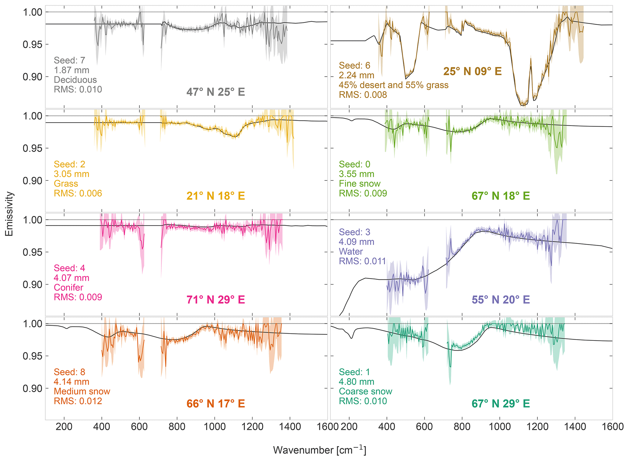
Figure 5 Retrieved emissivity for eight scenes with various surface types. The retrieved emissivity is shown as a dark coloured line, with the 1σ retrieval uncertainty range shown as a shaded region of the same colour. The true emissivity is shown as a solid black line in each figure, and the a priori emissivity is in grey. All retrievals use the baseline parameters from Sect. 3. Each scene uses atmospheric and surface data from the coordinates indicated on the figure for 15 January 2018 at 12:00 UTC. More information for each scene is listed in Table 1, and the true precipitable water vapour content and surface type is indicated on the figures. Each retrieval uses synthetic observations generated with a different random instrumental noise seed to mirror true retrieval conditions, and the seed is indicated on the corresponding figure. The retrieved emissivity is only shown in the spectral regions in which the information quantifier (see Eq. 5) is larger than 1, and the indicated root mean square error (RMS) is calculated in these regions.

While, in practice, FORUM users could be provided with the full retrieval and uncertainty vectors, in this work the criterion in Eq. (8) is used to ease interpretation. Figure 5 shows this retrieved emissivity product for eight dry geographic scenes with different surface emissivities. Only scenes with pwv below 5 mm are shown here to demonstrate the viability of FORUM FIR emissivity retrievals (for FEES emissivity retrievals of scenes with pwv higher than 5 mm, see Sgheri et al., 2022). As already seen in Fig. 3, the emissivity in dry scenes is retrieved in two sections above and below the CO₂ band, with the uncertainty in the retrieval highest in the edge regions of these sections. Figure 5 thus illustrates the potential of FORUM to retrieve FIR emissivity for a range of surface types and locations on the globe.

5 Impact on retrieval quality by precipitable water vapour

In this section, the analysis of the variation in the retrieval quality with water vapour content shown in Fig. 4 for the scene at 67^∘ N, 18^∘ E is extended and compared for multiple geographic scenes. The procedure for modifying the pwv content is identical. Leaving all other atmospheric and surface properties untouched, the climatological water vapour profile of the scene was multiplied by a constant value (ranging from 0.05 to 120). The four scenes (25^∘ N, 09^∘ E; 21^∘ N, 15^∘ E; 67^∘ N, 18^∘ E; and 67^∘ N, 29^∘ E) and the corresponding maximum and minimum water vapour profiles used can be seen in Fig. 6a. The synthetic observations generated from these modified scenes were then used to run the baseline retrieval (see Sect. 3). Although these modified scenes included some non-physical water vapour profiles, there was no significant change in the retrieval quality of the atmospheric profiles.

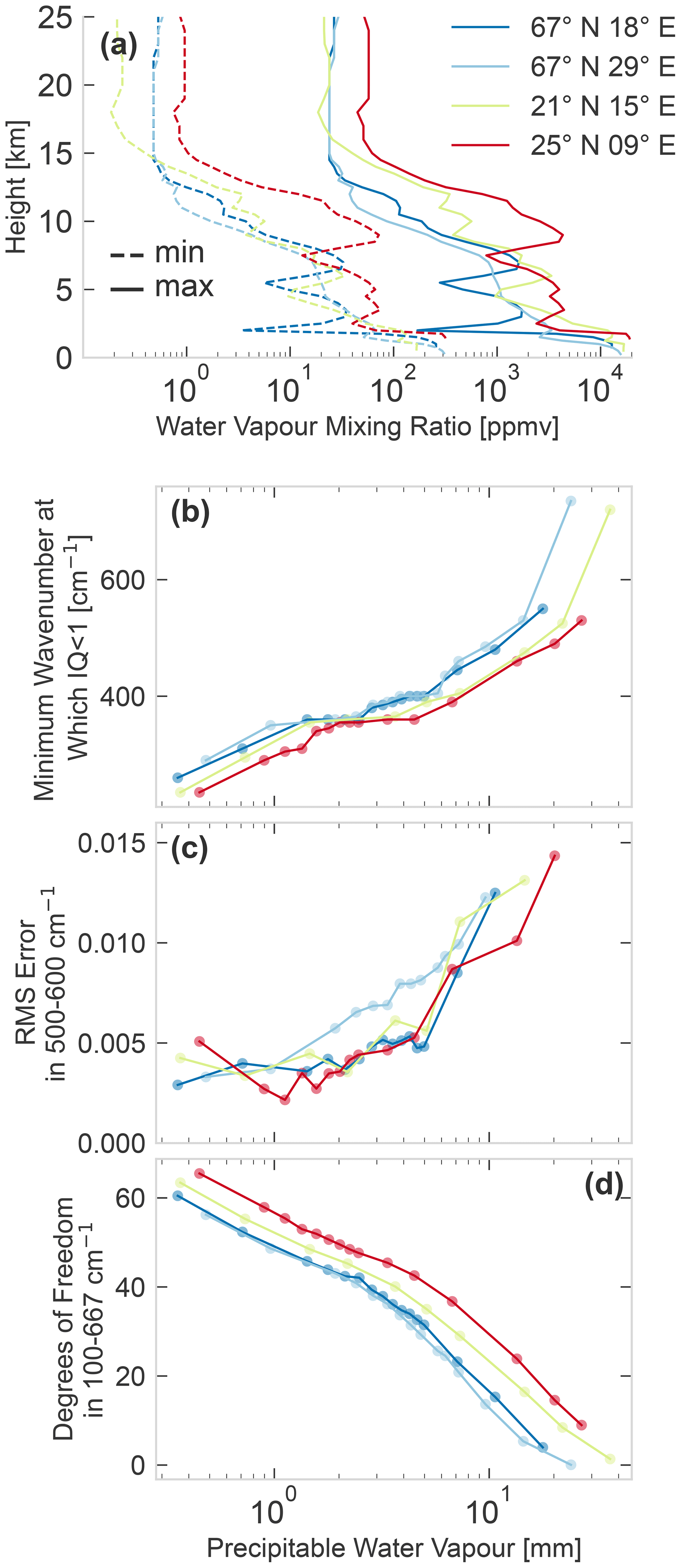
Figure 6 Retrieval quantifiers as a function of scene precipitable water vapour. For each scene, the climatological water vapour profile was multiplied by a constant factor when generating the synthetic observations so as to keep everything constant, except for the water vapour content. Panel (a) shows the minimum (dashed line) and maximum (full line) modified water vapour profile. Panels (b), (c) and (d) have a shared x axis showing the precipitable water vapour of each scene, with the colour coding of the lines and markers the same as in panel (a). Panel (b) shows the minimum wavenumber at which the retrieved emissivity satisfies the criterion in Eq. (8). Panel (c) shows the root mean square (RMS) error of the retrieved true emissivity in the 500–600 cm⁻¹ range for the cases with full sensitivity in that range (thus, even for this conservative range, the RMS is not calculated for the highest pwv values). Panel (d) shows the degrees of freedom in the 100–667 cm⁻¹ range (the sum of the emissivity averaging kernel submatrix rows corresponding to that range). All three figures show the quantifiers improve as the water vapour content decreases.

In Sect. 4, it was seen that as pwv decreased the retrieval quality at a given FIR wavelength improved as microwindows deepened and the retrieval sensitivity extended farther into the FIR as new microwindows opened up. To complement the spectral analysis of Fig. 4 and compare the variation in quality for multiple scenes, in this section three single-value quantifiers are analysed for the retrievals. All three are shown in Fig. 6 and plotted against the true pwv content of the scene.

Table 2 Data points from Fig. 6 for the case at 67^∘ N, 18^∘ E. Note: pwv is the true precipitable water vapour content of the retrieved scene, and the lowest sensitive wavenumber is the minimum wavenumber at which the retrieved emissivity satisfies the criterion in Eq. (8).

The first quantifier in Fig. 6b shows the lowest wavenumber of retrieval sensitivity into the FIR by plotting the minimum wavenumber which satisfies the criterion for retrieval (see Eq. 8). The data for 67^∘ N, 18^∘ E are also listed in Table 2. This wavenumber value decreases as the scene becomes drier and the weaker microwindows become transparent enough for the emissivity to be retrieved at lower wavenumbers. The second quantifier in Fig. 6c shows the root mean square (RMS) error of the retrieved emissivity in the 500–600 cm⁻¹ region for the cases that are fully sensitive in that region. While the region in which the emissivity is being retrieved in the FIR can be larger than 500–600 cm⁻¹ for many of these cases, the RMS is calculated for a constant region to avoid the influence from the fluctuations at the edge of the sensitive regions. Figure 6c shows that, not only does the lowest wavenumber of sensitivity decrease, but the retrieval quality also increases as the scene becomes drier. The final quantifier in Fig. 6d shows the degrees of freedom of the emissivity retrieval in the full 100–667 cm⁻¹ FIR region, calculated from the averaging kernel matrix. It is noteworthy that, unlike the other qualifiers which have occasional plateaus in their trends, the information content in the FIR increases monotonically as the pwv decreases.

All cases individually show the same improvement in quality, with pwv discussed in detail for Fig. 4, and the results are only weakly dependent on the scene. However, there is a small difference in the scene specific behaviour in all three plots, of which Fig. 6d gives the clearest view. In general, for the same value of pwv, 25^∘ N, 09^∘ E has the best retrieval quality, with 21^∘ N, 15^∘ E next in quality and 67^∘ N, 18^∘ E and 67^∘ N, 29^∘ E lowest and about equal in quality. Although the many parameters of the atmospheric state and the small number of scenes investigated make attribution of this difference difficult, a plausible explanation can still be identified. The difference in surface temperature and surface–atmosphere contrast between these scenes. The hot scenes are 25 and 21^∘ N (T_s>300 K; see Table 1), and their higher surface temperatures lead to a larger sensitivity to emissivity through the stronger T_s–emissivity correlation (see Sect. 6 and Appendix A). And though the 21^∘ N scene surface temperature is in fact 4 K warmer than the 25^∘ N surface temperature, the temperature contrast with respect to the atmosphere is 12.7 and 15 K in the scenes, respectively. A larger difference between the air and surface could mean that the surface emission is easier to separate from the atmospheric emission and would also reduce the reflected downwelling radiation. Further work should extend the analysis to a larger number of geographic scenes to better quantify this effect.

Overall, the analysis of Fig. 6 shows that FORUM measurements will provide significant information on emissivity in the FIR in a range of scenes.

6 The correlation of surface temperature and emissivity and its consequences

The difficulty in surface emissivity retrieval caused by the connection of emissivity to surface temperature is widely recognized in the field of remote sensing (Li et al., 2013). In many cases, one is only interested in either emissivity or surface temperature, but Eq. (3) shows that, from radiance measurements, these cannot be determined independently. Even if one is only interested in the surface properties, the difficulty in Eq. (3) arises from two sources, namely imperfect knowledge of 𝒯(z), the atmospheric transmittance between the surface and the instrument and at the measurement resolution the degeneracy of the surface emission itself with regards to the parameters of interest. The FEES retrieves the surface temperature and the atmospheric state that defines 𝒯(z) at the same time as the spectral emissivity. The contribution of water vapour to 𝒯(z) was discussed in Sects. 4 and 5. This section focuses on the T_s–emissivity correlation that arises from Eq. (3) and investigates its impact on the retrieved emissivity. To complement the general analysis of this section, the spectral dependency of this correlation strength is discussed in Appendix C.

6.1 Surface temperature and emissivity in the surface emission equation

The surface emission equation (Eq. 3), as written, is degenerate. Even if the atmospheric state is known and so L_d,σ is given, measurements of S_surf,σ at N wavenumbers still leave N+1 unknowns to solve for, i.e. N spectral emissivity values and the surface temperature T_s. The constraint is that the surface emissivity ϵ_σ≤1 checks this degeneracy and provides a lower bound for the retrieved T_s. However, for any higher values of T_s, it is possible to find a corresponding surface spectral emissivity ϵ_σ that produces the correct surface radiance.

Different methods have been developed to deal with this degeneracy in the MIR when it occurs (see Li et al., 2013 for a review). While most methods make assumptions or use empirical relations which cannot be extended into the FIR, as Murray et al. (2020) and Bellisario et al. (2017) have shown, MIR measurements can be used to retrieve a T_s, which can then be used for the FIR emissivity retrieval. Future work could investigate such methods by incorporating independent MIR measurements from synergy with the Infrared Atmospheric Sounding Interferometer – New Generation (IASI-NG) in tandem with the full-spectrum simultaneous OE retrieval used in this work.

In the FEES OE retrieval, the assumption that breaks the degeneracy of Eq. (3) is the retrieval of emissivity on a coarser grid than the measurements. As discussed in Sect. 4, the ∼ 0.4 cm⁻¹ spaced ϵ_σ used to calculate S_toa,σ is computed by linearly interpolating between the emissivity values retrieved on a coarser 5 cm⁻¹ grid. Thus, the retrieval vector $\widehat{\mathit{x}}$ has fewer elements than the observations vector y, and the retrieval is not ill-posed, only ill-conditioned. This interpolation uses the assumption that the emissivity is smooth, and so breaks the degeneracy in a similar way to the retrieval method seen in Murray et al. (2020) and Knuteson et al. (2004). If in the FEES OE forward model the emissivity and T_s move away from the true value, to keep S_surf,σ the same in Eq. (3), the spectral emissivity would have to take up a shape with sharp high-resolution spectral features corresponding to the spectral pattern of L_d,σ. These cannot be reproduced by the interpolated coarser grid, and so ξ² is larger value farther away from the correct emissivity. Thus, the smoothing means that an incorrect emissivity introduces errors in the forward model, and this penalization leads the algorithm to nudge the retrieval vector towards the true value.

However, for small shifts away from the true emissivity and true T_s, the errors introduced in S_surf,σ can be within the FORUM instrumental uncertainty. Thus, to a limited extent, the functional form of the emissivity and surface temperature still allows the retrieval to converge to a range of different emissivities. Such a parameter combination is sometimes called sloppy, as moving along a sloppy direction in the parameter space has little effect on the behaviour of the model (see Transtrum et al., 2011). The combination of T_s and emissivity form a sloppy valley in the model parameter space.

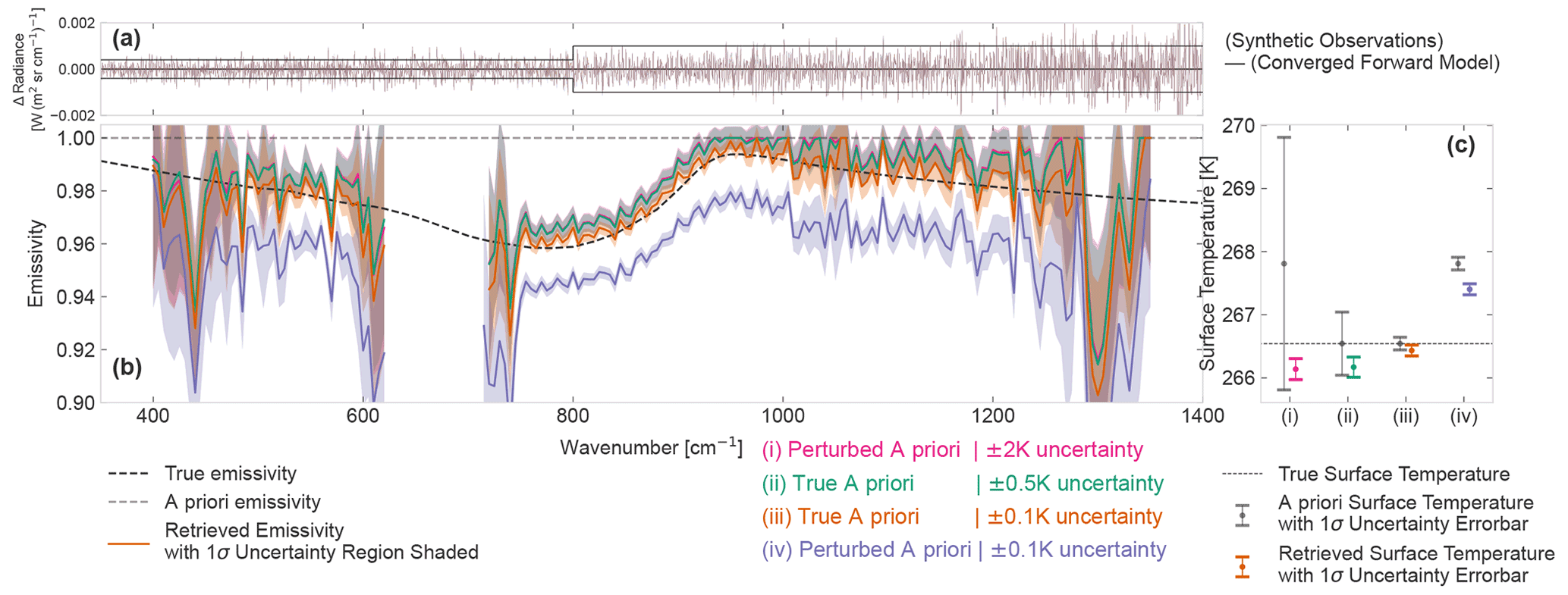
Figure 7 Different constraints on the surface temperature retrieval. Panel (b) shows the retrieved emissivity with the ±1σ retrieval uncertainty range shaded in the same colour. Panel (c) shows the retrieved surface temperatures with ±1σ retrieval uncertainty for the same retrieval runs as panel (b). Panel (a) shows the difference between the same synthetic observations and the four different converged forward models. The four cases are detailed in the text, and the retrievals are pink, green, orange and purple for cases (i), (ii), (iii) and (iv), respectively. Note that the scale in panel (b) only shows the emissivity from 0.9–1.0, and that even the wrongly constrained case (iv) only results in an uncertainty on a scale of ∼ 0.02.

Figure 7 is shown both as an illustration of how surface temperature and emissivity compensate for each other and as a comparison of different a priori constraint scenarios. The retrieval of scene 67^∘ N, 29^∘ E with instrumental noise seed 0 was specifically chosen for this figure due to the ∼ 0.01 shift seen in the default retrieval, and it is not necessarily a representative case.

As mentioned above, it is likely that, for operational FORUM retrievals, an estimate of T_s will be available either from independent observations, from synergy with IASI-NG, or from a different analysis of the FORUM observations. Thus, the retrieval is run for four different scenarios of the surface temperature a priori information, as follows:

• i.

  The default FEES retrieval, where a perturbation of the true T_s is used as a priori with a 2 K a priori uncertainty that is characteristic of surface temperature measurements.

• ii.

  To model the ideal scenario of correct and accurate independent measurements, the true T_s is used as both a priori and initial guess, with a smaller 0.5 K a priori uncertainty.

• iii.

  A similar but less realistic scenario in which a high confidence in the independent measurement of the true T_s means that the true value is set as both a priori and initial guess as in (ii), but in this case with a 0.1 K a priori uncertainty.

• iv.

  To test whether using a tight a priori constraint is advisable, the final retrieval uses the perturbed T_s of (i) as the a priori and initial guess, with the 0.1 K a priori uncertainty of (iii).

The first thing to note from the figure is the expected anti-correlation of the surface temperature and emissivity systematic uncertainties in the retrieved values. Out of the four cases, only retrieval (iii) has a retrieved surface temperature centred on the true value, with (i) and (ii) having lower and (iv) higher retrieved surface temperatures. These shifts in T_s cause upward/downward shifts of the whole spectral emissivity, with sign and size anti-correlated with the systematic uncertainty in surface temperature. It is interesting to note that, even though the emissivity retrieval is shifted for the different cases, the emissivity retrieval uncertainty is the same for all of them, and when examined, none of the standard quantifiers (see Fig. 3) show which retrieval is better than the other. The reason can be seen in Fig. 7a. All of these solutions are in the same sloppy valley of the parameter space and so reproduce the observations to the same accuracy within the FORUM goal noise. This illustrates the effect that the functional form (ϵB(T_s)) of T_s and emissivity in the forward model can have on the retrieval.

Are the imposed constraints on T_s useful for mitigating such compensating shifts and reducing the systematic uncertainty on emissivity? There are two points to be made from the cases in Fig. 7, as follows:

• Even a constraint of ±0.5 K around the true value of T_s does not correct the shift seen in the default retrieval and can still result in an emissivity retrieval in which the true emissivity is outside the ±1σ retrieval uncertainty range (but it should be noted that it is within both ±2σ and the goal FORUM emissivity uncertainty of ±0.01).

• Scenario (iii) shows that a constraint of ±0.1 K is sufficiently small to result in the correct retrieved emissivity. However, scenario (iv) shows that this is too tight of a constraint; if the a priori T_s value is inaccurate even by ±1.5 K, then this already causes a much larger shift in the retrieved emissivity than is seen in the default scenario with more freedom for T_s. It is, therefore, not recommended to use such a tight a priori constraint.

6.2 Impact on the retrieval by the a priori and initial guess choices

The retrievals shown in the previous section investigated possible T_s a priori constraints. This section investigates the impact allowed by the correlation of surface temperature and emissivity when varying the value of the emissivity initial guess and a priori without changing the a priori uncertainty constraints.

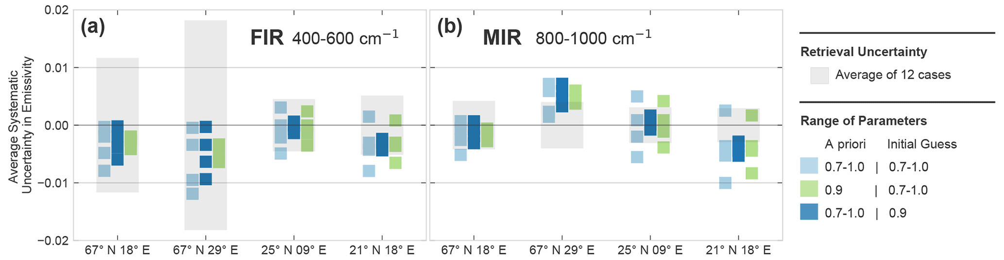
Figure 8 Systematic uncertainty in emissivity retrievals caused by the different choice of emissivity a priori or the initial guess for four geographical scenes. Except for the choice of emissivity initial guess and a priori, all details can be found in Sect. 3. The coloured squares show the spectrally averaged value of systematic uncertainty in the retrieved emissivity for different variations of the parameters. Panels (a) and (b) show the average values in 400–600 and 800–1000 cm⁻¹, respectively. In dark blue, the initial guess is kept constant at 0.9, and the a priori takes the values of 0.7, 0.8, 0.9 and 1.0. In light green, the a priori is kept constant at 0.9, and the initial guess takes the values of 0.7, 0.8, 0.9 and 1.0. In light blue, the a priori and initial guess take the same values of 0.7, 0.8, 0.9 and 1.0. For reference, the average value of the 1σ retrieval uncertainty from all 12 parameter combinations is shown as a dashed grey region in the background. Note that the ranges in all four figures are very small in extent, and the scale of the y axis is ±0.02 to highlight the differences.

To explore the individual effects of the emissivity a priori and initial guess on the retrieved emissivity, their values are varied independently. The baseline retrieval was run for a combination of different constant a priori cases and initial guesses for four different geographical scenes, and the results are shown in Fig. 8. The impact of the different combinations is shown by shading in the range between the maximum and minimum of systematic uncertainties in the retrieved emissivities for three colour-coded scenarios, as well as shading in the maximum retrieval uncertainty range in grey. These scenarios are as follows:

• The initial guess is kept constant at 0.9, and the a priori is varied in steps of 0.1 from 0.7 to 1.0.

• The a priori is kept constant at 0.9, and the initial guess is varied from 0.7 to 1.0.

• The initial guess and a priori take on the same value and are jointly varied from 0.7 to 1.0.

While this is not an exhaustive list of the possible a priori/initial guess combinations in the 0.7–1.0 range, the maximal impact that combinations in this range can have are represented by the difference between the case where both the a priori and initial guess are 0.7 and that when they are both 1.0.

Note, however, that all these retrievals are run for the same default instrumental noise seed, and so the specific higher/lower value of the retrieved emissivity is not necessarily characteristic. An in-depth analysis would average retrievals run for at least 100 different versions of random instrumental noise and varying the L2M random seed, but this is outside the scope of the slow line-by-line forward model used by the L2M (which prioritizes accuracy). On the other hand, the choice of instrumental random noise should not affect the magnitude of the resulting emissivity ranges or their relation to each other, which is what is examined in this section (to confirm this, the above analysis was in fact repeated for a small number of seeds and showed similar results, with the ranges shifted up or down by a small amount). A full analysis would also consider different a priori uncertainties (see Appendix B) and T_s retrieval parameters.

Figure 8 shows the same full-spectrum upward/downward shifts in emissivity that were seen in Fig. 7. In all of the scenes, the impact of the a priori/initial guess variation is not large overall, and the full range of variation amounts to, at most, a 0.015 relative difference in emissivity. The full range also appears to be additive in the impact of the two parameter choices (i.e. the range of the joint variation is the sum of varying each parameter individually).

However, the relative and total size of the ranges show a different behaviour in scenes 67^∘ N, 18^∘ E and 67^∘ N, 29^∘ E than in scenes 25^∘ N, 09^∘ E and 21^∘ N, 18^∘ E. While in the first two the variation of initial guess has slightly less of an influence than the a priori, in the third and fourth the sensitivity to the initial guess is stronger. This would not, in general, be expected from an OE retrieval, where usually the initial guess has little influence. However, the effect of the initial guess choice seen in Fig. 8c and d​​​​​​​ is not due to a false convergence of the retrieval, and the final forward model of all the retrievals for a given scene is almost identical. Thus, they have the same final χ² (see Eq. 1) and reach convergence in the same way. This is the same process that was seen in Fig. 7a, where the shifts in T_s and emissivity compensate for each other in a way that results in the same forward model within the FORUM noise. We can conclude that the sloppy valley of emissivity and T_s allow for a small range of solutions around the true value, and the choice of initial guess gives the retrieval a small nudge within this range.

The different behaviour in the four scenes is likely due to their geophysical characteristics. While 67^∘ N, 18^∘ E and 67^∘ N, 29^∘ E both have low surface temperatures and a low surface-to-air temperature contrast, 25^∘ N, 09^∘ E and 21^∘ N, 18^∘ E are hot scenes with high surface temperatures and a high surface-to-air temperature contrast (see Table 1). This means that the latter two have a stronger correlation of surface temperature with emissivity, and so the retrieval vector can take larger steps in the parameter space. This effect of the path on the solution is discussed and analysed in more detail in Appendix A. For the purpose of this section, it is sufficient to note that, although the range is at least twice as large for the hotter scenes, even in the worst-case scenario the choice of initial guess and a priori only change the emissivity by about 0.015, which is still close to the FORUM goal accuracy of 0.01.

While these shifts are not in themselves problematic, the cases where the retrieval uncertainty ranges in Fig. 8 are smaller than the parameter-variation-induced ranges require further investigation. This discrepancy occurs because the emissivity a priori is affecting the retrieved emissivity indirectly through the T_s sloppy valley, and such an indirect effect is not represented in the standard uncertainty analysis which only uses the diagonal elements of S_x and the emissivity submatrix of A. Therefore, to produce a reliable emissivity retrieval product, further work is needed to develop an uncertainty analysis which quantifies this indirect effect.

7 Conclusions and recommendations

This study follows from previous work on FORUM geophysical retrievals (e.g. Ridolfi et al., 2020; Sgheri et al., 2022), showing that FORUM measurements will be able to provide retrieved surface emissivity in a significant region of the FIR. Using the FEES, factors that influence OE retrievals of FIR emissivity were investigated with an emphasis on the development of operational retrievals for FORUM. More information could be gained from the retrieval by analysing individual scenes in detail and combining the OE retrieval with different methods, and this should be addressed in future work. Additionally, we have only considered the use of FORUM measurements by themselves (see Ridolfi et al. (2020) for a discussion of how synergetic retrievals with IASI-NG observations can improve the FORUM geophysical products).

In Sect. 4, the retrieved emissivity was introduced together with the quantifiers used to analyse it. In Sect. 5, the variation in the quality of the retrieval with pwv content was compared for multiple geographic scenes. Section 6 then investigated the consequences and characteristics of the surface temperature–emissivity correlation that arises from the functional form of the surface emission equation.

This work has shown the following:

• Emissivity retrieval quality, degrees of freedom and extent of retrieval sensitivity towards shorter wavenumbers increase as the pwv of the scene decreases.

• For the cases investigated here, varying the value of the emissivity a priori and initial guess between 0.7 and 1.0 results in relative differences in the FIR retrieved emissivity of up to 0.015 in the extreme.

In addition, the following recommendations can already be made for FORUM emissivity retrievals based on this work:

• When using the FORUM geophysical emissivity product, the spectral extent of the emissivity used for analysis should be decided on a scene-by-scene basis (and not, for example, by applying a latitude cutoff). We recommend using the information quantifier of the scene as a basis for evaluation.

• The functional form of the surface emission equation leads to a strong anti-correlation of surface temperature and emissivity in the retrieval. Thus, the retrieval can converge to a small range of solutions around the true value. Attempting to correct this by constraining the surface temperature retrieval (i.e. introducing more a priori information) could lead to larger shifts away from the true emissivity when the a priori for the surface temperature T_s is wrong. Thus, a surface temperature a priori uncertainty of ± 2 K is recommended, as, even in the worst cases investigated here, it only results in an emissivity offset of an acceptable value around 0.01.

In order to best utilize FORUM measurements to retrieve emissivities, the following two recommendations are made for the development of the FORUM emissivity retrieval:

• The quality of the retrieval varies greatly depending on scene parameters such as the water vapour content, absolute surface temperature and its contrast to the atmospheric temperature. These scene dependencies should be investigated in order to identify the best conditions for retrieval of FIR emissivity.

• The correlation of emissivity with T_s leads to offsets in both retrieval parameters that are not accurately reflected in the standard quantifiers. It is recommended that the systematic uncertainty originating from the T_s–emissivity correlation is evaluated in detail during the development of the operational retrieval. Further work could also look into the possibility of using external constraints on T_s and other methods for T_s retrieval (such as those used in Murray et al., 2020) to complement the OE.

In addition to these two steps, complementary future work would include laboratory and aircraft measurements of emissivity, analysis of additional methods for surface temperature retrieval and an algorithmic optimization of the emissivity retrieval grid. In addition, after the launch of FORUM, a progressively better emissivity product can be obtained as emissivity climatologies are developed both from FORUM radiances and other FIR measurements.

In conclusion, the FORUM mission will be able to provide a unique contribution to our knowledge of surface emissivity in the FIR for many locations on the globe and, potentially, most types of surfaces. In this work, we have taken the first steps towards the development of an operational emissivity geophysical retrieval for the FORUM mission by highlighting possibilities for optimization of the retrieval and the systematic uncertainties that still need to be quantified.

Appendix A: The retrieval path in the emissivity-T_s parameter space

In Sect. 6 of the paper, the concept of the T_s–emissivity parameter space and its sloppy nature was introduced in the context of the surface emission equation (Eq. 3). The OE retrieval algorithm in the FEES minimizes the cost function (Eq. 1) using the Levenberg–Marquardt approach which interpolates between the Gauss–Newton algorithm and the method of gradient descent. The retrievals in this work converge after four to six iterations, and convergence is reached when the normalized change from one iteration to the next in χ² (the first term in Eq. 1) is less than 0.01. The path that the retrieval takes to convergence is hard to visualize, as the retrieval vector is stepping in a 300+ dimensional parameter space. However, due to the linear contribution of emissivity to the TOA radiance (see Eq. 3), insight can be gained by plotting the steps in the surface temperature–emissivity slice of this parameter space, and two such plots are shown in this appendix. While the full forward model is far too complex and its computation too time-consuming to lend itself to contour plots or manifold visualizations, some insight can also be gained by showing these steps together with the contours of constant surface emission in Eq. 3.

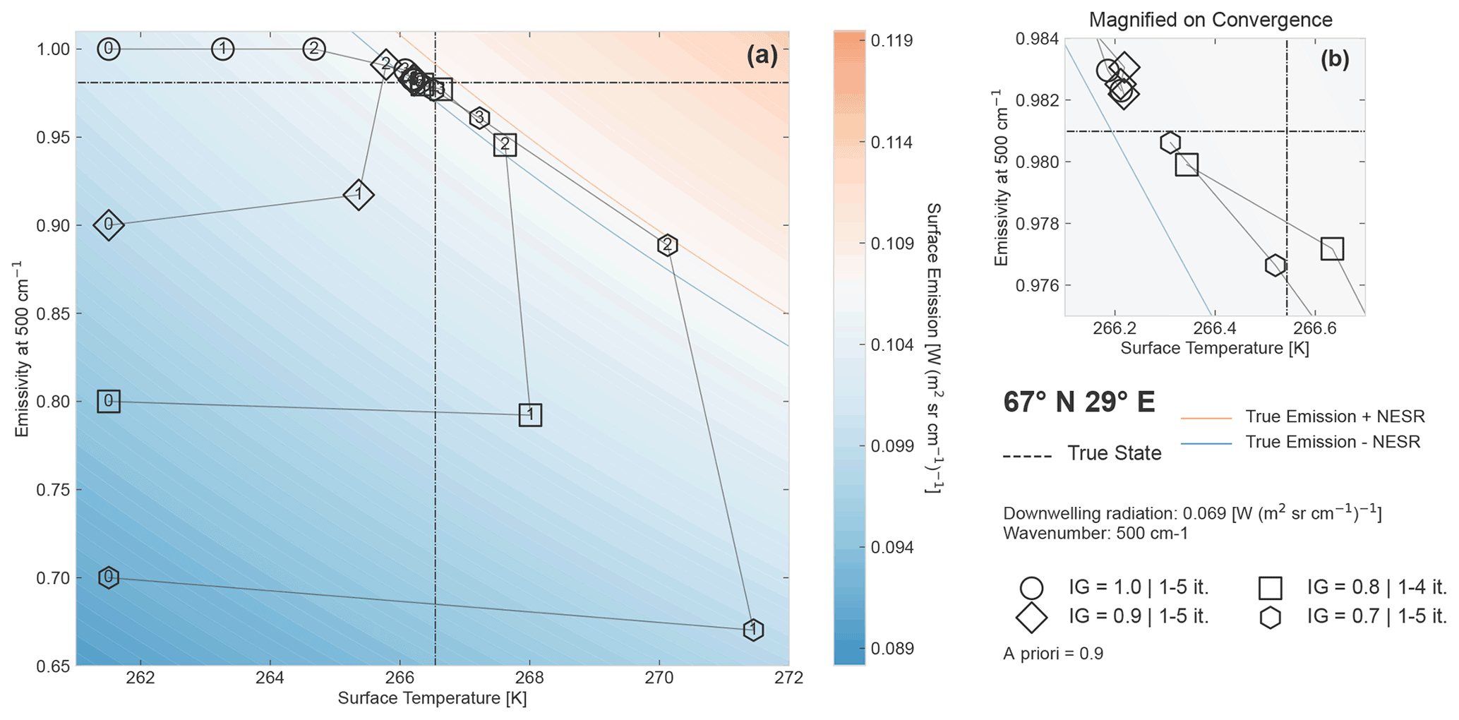
Figure A1 The value of the two elements of the retrieval vector for all retrieval iterations in the emissivity, with the surface temperature (T_s) parameter space for the 67^∘ N, 29^∘ E coarse snow scene. Panel (a) shows the parameter space defined by T_s and the emissivity at 500 cm⁻¹, with coloured contours corresponding to the surface emission at 500 cm⁻¹ (according to Eq. 3), with the downwelling radiation set to the true value of 0.069 W (m² sr cm⁻¹)⁻¹. The centre of the diverging colour scale is the true value of the surface emission. The true values of emissivity and surface temperatures are shown in dashed black lines. An orange (blue) line shows the contours of the true emission plus (minus) the FORUM noise equivalent spectral radiance (NESR) in the FIR. The different geometric marker shapes show the retrieval vector values for the iterations of four different retrievals, starting from the initial guess until the converged solution. In the four cases shown, the emissivity a priori is 0.9, and the initial guess takes the value of 1, 0.9, 0.8 and 0.7, as shown with circles, diamonds, squares and hexagons, respectively. All other retrieval parameters are the same for the four cases and are the default values outlined in Sect. 3. Panel (b) shows an enlarged portion of panel (a) centred on the true state for a clearer view of the later iterations (the colour scale and all other plotted values are the same as in panel a). The full spectral range of the final retrieved emissivity values for the four runs is shown in Fig. 8 in Sect. 4 of the paper.

The issue addressed in this paper which benefits most from such parameter space path plots is that of the sensitivity of the retrieval to the initial guess discussed in Sect. 6.2. Figure A1 shows the convergence of the retrievals shown as the light green range in Fig. 8b, in which the emissivity of scene 67^∘ N, 29^∘ E is retrieved with an a priori of 0.9 and different initial guesses of 0.7, 0.8, 0.9 and 1.0. For each iteration, Fig. A1a plots the value of two retrieval vector components, with the surface temperature on the x axis and the emissivity at 500cm⁻¹ on the y axis. The four different retrieval runs are represented by different geometric shapes. To put the convergence into context, Eq. (3) is used to plot the contours of the true surface emission value for each T_s–emissivity combination. For simplicity, the surface emission is calculated at the surface (without the atmospheric transmission term). L_d is taken to be the true value at 500 cm⁻¹, calculated using a separate run of LBLRTM (version 12.10) using the true atmospheric state of the scene. Note that, as the atmospheric profiles are also being retrieved, both the transmission and L_d in the forward model will not necessarily equal the true values at the early iterations, and so the background contours do not represent the surface emission used in the forward model at that iteration but instead are there to give context to the later iterations (where the retrieval vector is close to the true). In addition, these contours are not directly representative of the forward model, as f(x) includes many additional effects (for example, those associated with the FORUM instrument). Finally, in Fig. A1b, a small region of the space has been magnified so as to better show the behaviour around convergence.

The behaviour of the different retrievals in Fig. A1 is typical of the emissivity retrieval. The retrieval vector starts from an initial guess, which corresponds to a surface emission very different from the true value, and so takes large steps in the parameter space towards the correct surface emission contour (this is the gradient descent part of the Levenberg–Marquardt minimization). The existence of this true surface emission contour is the cause of the sloppy valley in the T_s–emissivity space discussed in Sect. 6. While, in the MIR, the contour is usually reached in one step, in the FIR the retrieval usually takes two to three steps to reach the true emission value, as a change in the water vapour part of the retrieval vector also changes L_d. Once the true surface emission contour is reached, the retrieval proceeds along it, driven mainly by the T_s a priori constraint and by the small forward model discrepancies caused by the emissivity smoothness assumption (discussed in Sect. 6 and difficult to visualize when plotting only the retrieval vector emissivity components). The main point seen in Fig. A1 is that the direction of the shift of the final values from the true ones depends on whether the correct surface emission contour is first reached at a higher or lower value than the true emissivity (so that, even though a retrieval might start from an emissivity at 0.9 that is lower than the true value, due to the structure of the parameter space, it will reach a final value that is higher than the true value).

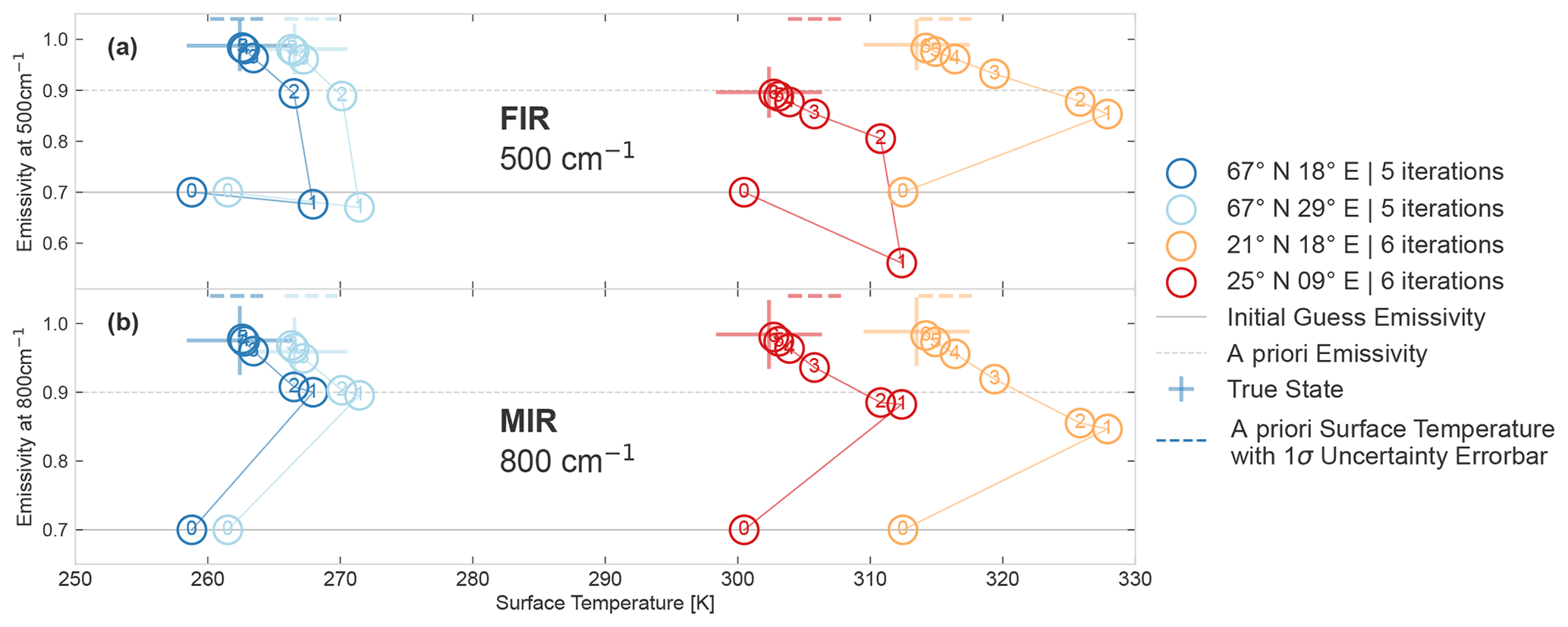
Figure A2 Value of two elements of the retrieval vector for all retrieval iterations in the emissivity, with surface temperature (T_s) parameter space for four different scenes. The four colour-coded scenes are shown (67^∘ N, 18^∘ E; 67^∘ N, 29^∘ E; 21^∘ N, 18^∘ E; and 25^∘ N, 09^∘ E) in dark blue, light blue, orange and red, respectively, with details as outlined in Sect. 3. The structure of the figure is similar to that of Fig. A1. For the four retrievals, the scattered coloured circular markers show the values of the emissivity and T_s at each numbered iteration of the retrieval starting from the initial guess until the converged solution. The retrieval parameters are the same for all scenes, with an emissivity a priori of 0.9 and an initial guess of 0.7 (all others have the default values outlined in Sect. 3). The y axis of panels (a) and (b) show the value of the emissivity at 500 and 800 cm⁻¹, respectively, with a shared x axis showing the surface temperature. Both figures also show the a priori emissivity and initial guess emissivity as dashed and solid grey lines, respectively. The different ±1σ a priori uncertainty range for T_s is shown as a dashed line at the top of the plot (the y-axis location has no significance other than clarity), with the same colour coding as the circular markers. This colour-coding is also used for the solid cross centred at the true values of emissivity and T_s of the scenes.

In Sect. 6.2, Fig. 8 the comparison for the initial guess sensitivity for different geographical scenes revealed a different behaviour of the colder 67^∘ N, 18^∘ E and 67^∘ N, 29^∘ E scenes and the warmer 25^∘ N, 09^∘ E and 21^∘ N, 18^∘ E scenes. The warmer scenes showed more sensitivity to the initial guess, in that there was a larger difference between the retrieved emissivity for different initial guesses. Figure A2 shows the convergence path of these four scenes in the FIR and MIR for the case when the initial guess emissivity is set to 0.7 (and the a priori is 0.9, as before). In this figure, no surface emission contours are shown, as their different L_d values mean that the contours would differ for the four different scenes. Figure A2 shows that, as discussed in Sect. 6.2, for the warmer scenes, the retrieval vector takes larger initial steps in the parameter space in both spectral ranges. This is what we would expect from the stronger correlation associated with the warmer scenes, which are analysed in detail in Fig. C1. Once the true surface emission contour is reached, the steps are of similar magnitude for the four scenes. Figure A2 illustrates how such larger steps in the first iteration could potentially explain a higher sensitivity to the initial guess. By taking a larger initial step, the retrieval approaches the true value from a lower emissivity value and so also converges to a slightly lower emissivity value.

In summary, plotting the retrieval's path to convergence in the emissivity-T_s parameter space is a useful visualization tool. By comparing the paths of different cases, it can provide further insight into the reasons underlying the sensitivity of the final retrieved product to different parameters.

Appendix B: Choice of a priori uncertainty

Throughout this work, the same emissivity a priori uncertainty matrix S_a was used for all retrievals. Its value was chosen as a baseline case, following the sensitivity tests shown in this Appendix.

In the FEES, S_a is calculated using two parameters, namely the uncertainty and the correlation length. For the profiles, the existence of reliable a priori datasets justifies a nuanced calculation of the uncertainty matrix using uncertainty and correlation lengths that change with height (see Sgheri et al., 2022). As there are no such datasets for FIR emissivity, as a starting point for optimizing the uncertainty, the same parameters are used for the full spectral range. Therefore, a constant uncertainty Δϵ and correlation length CL can be defined, and the S_a matrix elements for emissivity are then as follows:

$$\begin{array}{}\text{(B1)}& {\mathbf{S}}_{\text{a},ij}=\mathrm{\Delta }{\mathit{ϵ}}^{\mathrm{2}}\exp \left(-{\displaystyle \frac{\mathrm{\Delta }{\mathit{\sigma }}_{ij}}{\text{CL}}}\right),\end{array}$$

where Δσ_ij is the wavenumber difference between the location of the retrieved emissivity values ϵ_i and ϵ_j. In practice, Δϵ defines the freedom of the retrieval discussed in Sect. 3, as a larger value will allow the profile to take larger steps at each iteration and reduces the penalization from x−x_a. The CL controls the off-diagonal elements in S_a; its presence means that the regularization term for the retrieved emissivity points is not minimized individually but that the emissivity step at a given wavenumber is also affected by the difference of its neighbouring points from the a priori. In practice, this results in a smoother solution where the retrieval is sensitive to the a priori.

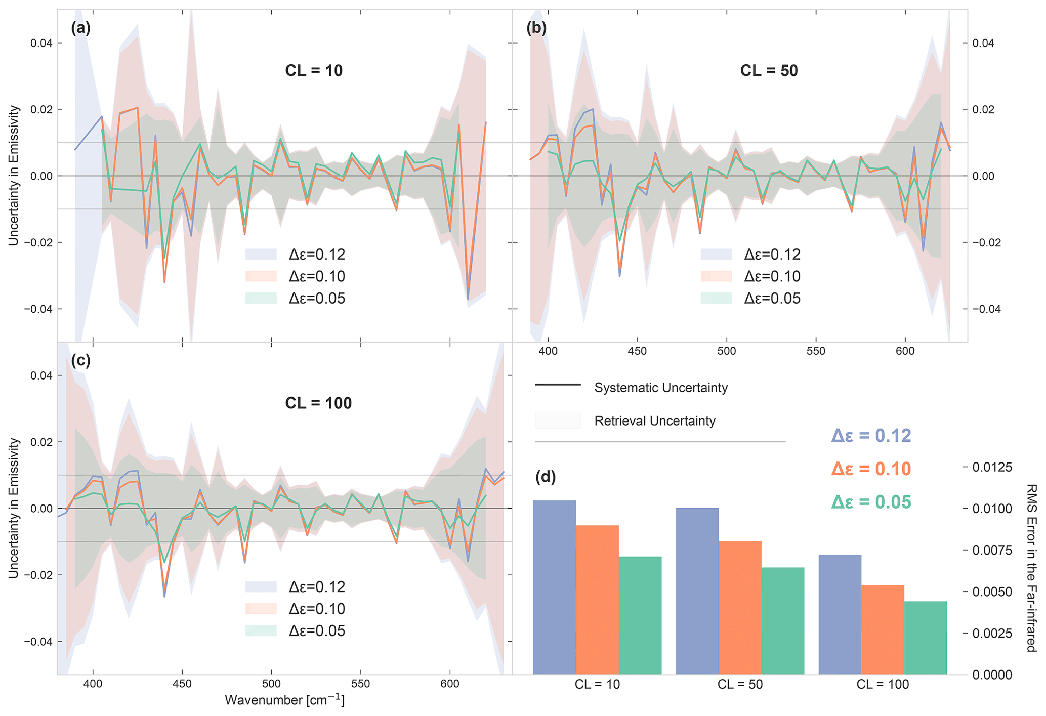
Figure B1 Systematic uncertainty in emissivity for different emissivity a priori uncertainty parameters in the far infrared. All nine retrievals are for the same fine snow emissivity at 67^∘ N, 18^∘ E on 15 January 2018 at 12:00:00 UTC, with the default parameters as outlined in Sect. 3. Panels (a), (b) and (c) show the uncertainties for retrievals with a correlation length (CL) of 10, 50 and 100, respectively. Each figure shows the systematic uncertainty (true minus retrieved emissivity) as a solid line for three values of the emissivity a priori uncertainty Δϵ. The colours are green, orange and blue for Δϵ values of 0.05, 0.1 and 0.12, respectively. The retrieval uncertainty 1σ range for the respective retrievals is shown as a shaded region of the same colour. The uncertainties are shown only in the regions where the information quantifier for the respective retrievals is larger than 1 (not the same for each retrieval) between 350 and 650 cm⁻¹. Panel (d) shows the root mean square (RMS) error of the systematic uncertainty in the plotted spectral range for the nine cases.

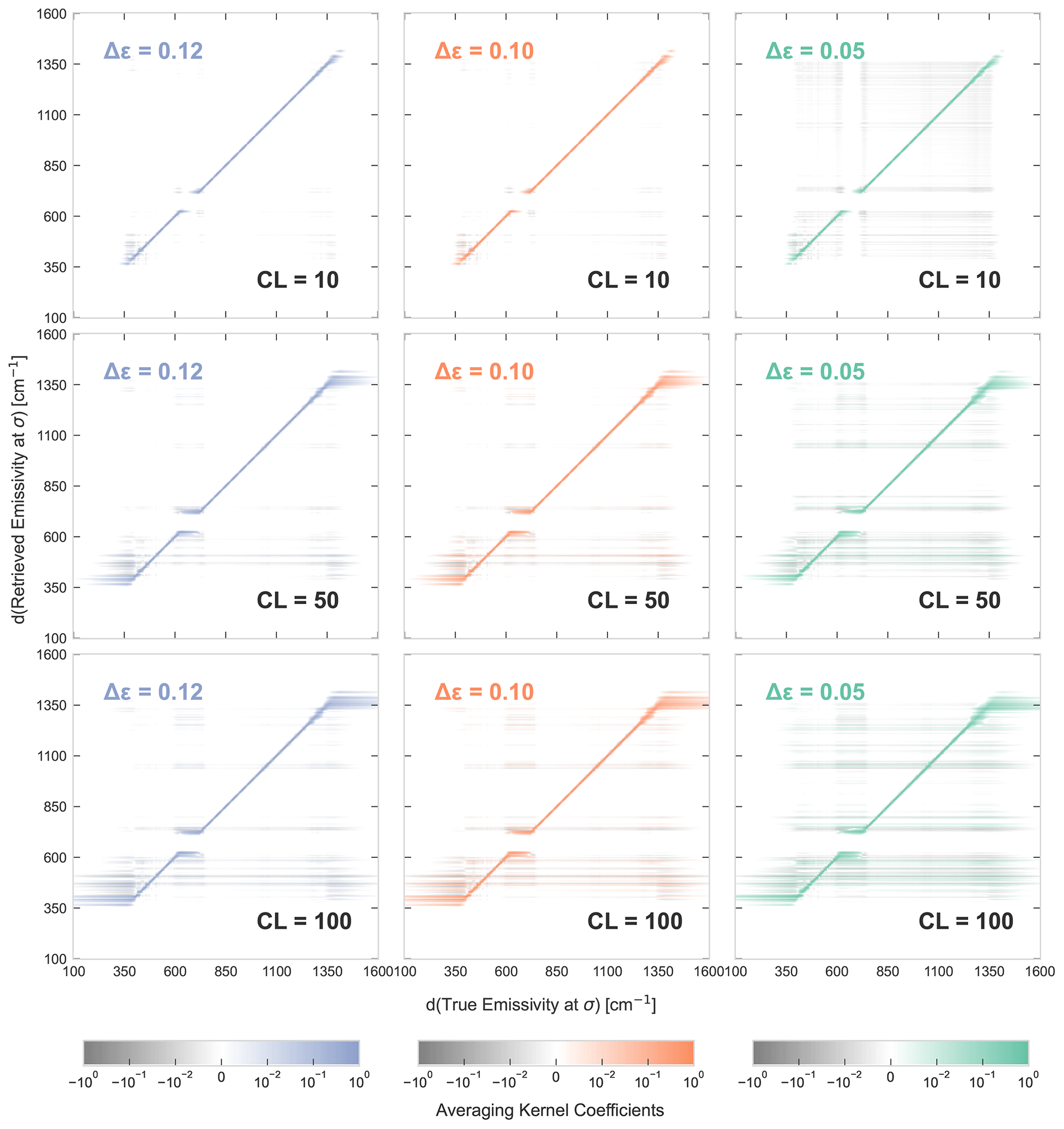
Figure B2 Averaging kernel coefficients (see Eq. 7) for the same nine cases shown in Fig. B1. The colour coding of the emissivity a priori uncertainty Δϵ is kept the same as Fig. B1, and its value is 0.12, 0.1 and 0.05 for columns 1, 2 and 3, respectively. Rows 1, 2 and 3 show cases with a correlation length (CL) of 10, 50 and 100, respectively. The colour scales are shown at the bottom of each column and are the same for each figure. The values are plotted with a lower threshold of $\pm {\mathrm{10}}^{-\mathrm{3}}$ for visibility.

These two parameters were varied in the retrieval set-up, and the results are shown in Figs. B1 and B2. While the sensitivity tests were run for many different scenes, the analysis shown here is of the scene at 67^∘ N, 18^∘ E, which was chosen as it is representative of the snow emissivity scenes that are the primary goal of FORUM's emissivity retrievals. The range of the uncertainty parameters shown is Δϵ=0.05, 0.1 and 0.12 and CL = 10, 50 and 100 cm⁻¹. Smaller values of Δϵ were also considered but are not shown as they did not give the retrieval the necessary freedom to converge to the right solution and caused a large systematic uncertainty. Figure B1 shows the systematic uncertainty and the retrieval uncertainty in the FIR for all nine cases and the root mean square (RMS) error for the systematic uncertainty values shown. Figure B2 shows the averaging kernels of the nine cases for the full spectral range. The following points can be seen in these figures:

• The differences in uncertainties for a given correlation length are only present in the edge regions of the retrieval, where the sensitivity is lower. This is because the a priori uncertainty only matters where information is drawn from the a priori, and for a dry scene such as this (as discussed for Fig. 3) in the centres of the FIR dirty window and of the MIR atmospheric window, the retrieval is fully sensitive to the true state, and thus the choice of a priori uncertainty has no influence.

• Examining the averaging kernels shown in Fig. B2, we can again see that the influence of the parameters is strongest at the edge regions of sensitivity. Here it can be seen that increasing CL leads to more information being drawn from regions to which the TOA is not, in reality, sensitive. Analysing the rows in the figure shows that decreasing Δϵ decreases the diagonal averaging kernel values and increases its off-diagonal values.

These averaging kernels show that the lower RMS error of the high CL and low Δϵ cases comes at the price of sensitivity to the true emissivity. In an ideal case, the averaging kernel is a straight diagonal line. The more spread out the edges of this line are, the more a priori information was used.

The main conclusion of this analysis is that there is no abrupt transition in the explored a priori uncertainty parameter space. All the parameter choices produced similar retrieval results, with differences only in less-sensitive regions. Therefore, a choice in either direction will either give slightly more sensitivity or accuracy and can be tuned to match the specific need of the user.

An additional option is to use a posteriori regularization. Using a larger error and a smaller correlation length would be desirable to give the retrieval more precision and freedom. As seen in this Appendix, due to the ill conditioning of the retrieval, the weaker regularization would cause the solution to oscillate more. An a posteriori regularization method, such as the IVS (iterative variable strength) method introduced in Ridolfi and Sgheri (2011) and applied to the FORUM atmospheric profile retrievals in Sgheri et al. (2020), could be used to smooth out these unphysical oscillations.

For the purpose of this study, Δϵ=0.1 and CL = 50 were used as the baseline parameter combination that represents a compromise between the two extremes of sensitivity and accuracy.

Appendix C: Spectral dependence of the emissivity-surface temperature correlation

To complement Sect. 6, the final step in understanding the variations allowed by the T_s–emissivity sloppy valley is to analyse the correlation strength in different spectral regions. Equation (3) shows that there are two main factors that could cause differences in the correlation in the FIR and MIR. The first originates from B(T_s) having a different shape in different spectral regions. The second is that, even if the downwelling radiation L_d is known, its value still differs significantly between the FIR and MIR. This is for the same reasons as discussed in Sect. 4. In the MIR, the atmospheric window is transparent, and so L_d is negligible, while in the FIR, L_d is higher or lower, depending on the amount of water vapour and on the microwindow structure (see, e.g., Palchetti et al., 2016, 2020 for ground measurements of FIR downwelling radiation).

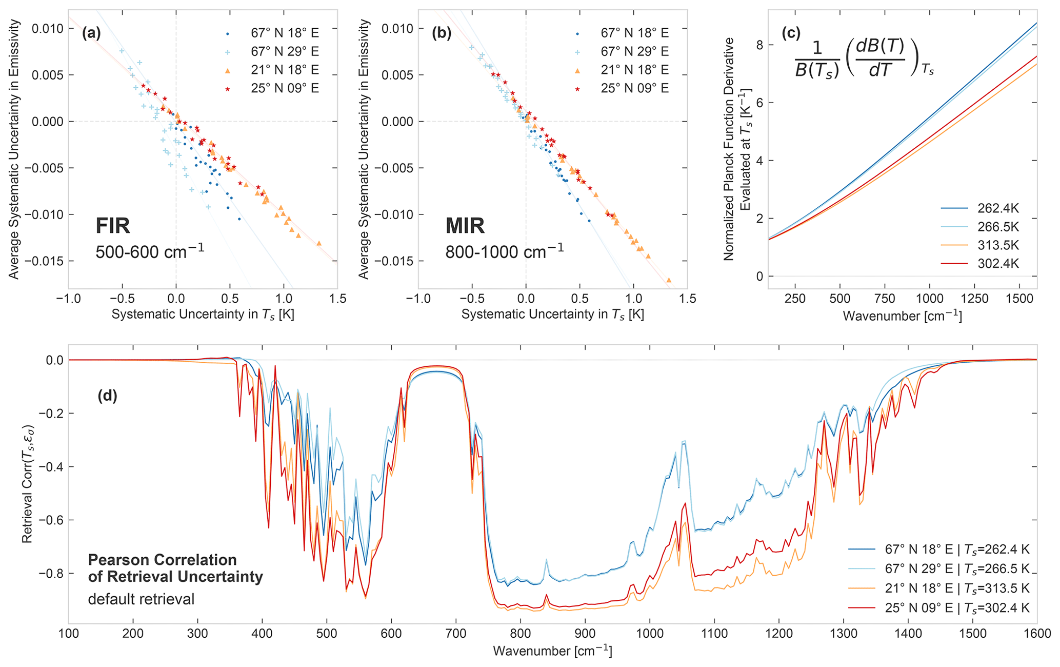
Figure C1 Correlation between emissivity and surface temperature in the atmospheric state retrieval. The four colour-coded scenes are shown (67^∘ N, 18^∘ E; 67^∘ N, 29^∘ E; 21^∘ N, 18^∘ E; and 25^∘ N, 9^∘ E) in dark blue, light blue, orange and red, respectively, with details as outlined in Sect. 3. Panels (a) and (b) show the retrieval systematic uncertainties for 28 retrievals of each scene. The baseline retrieval is run on spectra generated with six versions of random instrumental noise (seeds of 0 to 6) and for equal flat a priori cases and an initial guess set to 0.7, 0.8, 0.9 and 1.0. In panel (a), the average systematic uncertainty in emissivity in the 500–600cm⁻¹ range is plotted against the systematic uncertainty in the surface temperature (T_s). Light grey dashed lines show the true emissivity and T_s. Table C1 details the slope of the linear trend fitted to the points (grouped by scene) and the sample Pearson's correlation coefficient (see Eq. C1) for these data. The fitted trend is also plotted as a light line of the same colour as the corresponding data. Panel (b) is similar but with the 800–1000cm⁻¹ systematic emissivity uncertainty on the y axis. Its slope and correlation values are also detailed in Table C1. Panel (c) shows an analytic calculation of the value of the normalized Planck function derivative $\left[\text{d}B\right(T)/\text{d}T{]}_{T_{\text{s}}}/B(T_{\text{s}})$ at the four different true surface temperatures of the scenes, plotted over the full FORUM spectral range. Panel (d) shows the analytic Pearson correlation coefficient (see Eq. C4) of the emissivity and T_s retrieval uncertainty over the full FORUM spectral range for all four cases from the retrieval run, using the default setting outlined in Sect. 3. The correlation is calculated, as shown in Eq. (C4), from the retrieval uncertainty covariance matrix at convergence (see Eq. 4).

To investigate these effects, Fig. C1 shows an analysis of both the empirical correlation of the 28 retrieved values for four scenes each and an analytic correlation calculated from the standard OE equations. The same geographic scenes are used as in Fig. 8. For the empirical correlation, the baseline retrieval is run for each scene using instrumental spectra with seven different versions of random instrumental noise (generated with FSI seeds of 0, 1, 2, 3, 4, 5 and 6) and then each is retrieved with equal flat a priori cases and initial guesses set to 0.7, 0.8, 0.9 and 1.0, resulting in 28 cases for each scene. The variation in the instrumental noise and the a priori and initial guess results in a range of different systematic uncertainties (as discussed in Sect. 6.2). These uncertainties are shown in Fig. C1a and b, which plot the average systematic uncertainty of emissivity in a specific spectral range against the systematic uncertainty in T_s. Constant and relatively small spectral ranges are chosen so that the variation in the correlation slope and strength in the averaged range is small enough to allow a meaningful analysis. The spectral ranges of 500–600 and 800–1000 cm⁻¹ are chosen to represent the FIR and MIR, respectively, as these are the spectral intervals with the highest sensitivity in those regions. These are not representative of the variation in the full FIR/MIR but only indicative of the difference between the regions.

As expected, there is a strong anti-correlation between the systematic uncertainties both in the FIR and the MIR. Table C1 lists the slopes of the linear trends fitted to the data in these figures (grouped by scene and spectral region) and the corresponding sample Pearson correlation coefficient R using the standard formula, as follows:

$$\begin{array}{}\text{(C1)}& R={\displaystyle \frac{\sum \left(\mathrm{\Delta }{T}_{\text{s}}-m_{\mathrm{\Delta }{T}_{\text{s}}}\right)\left(\mathrm{\Delta }\mathit{ϵ}-m_{\mathrm{\Delta }\mathit{ϵ}}\right)}{\sqrt{\sum {\left(\mathrm{\Delta }{T}_{\text{s}}-m_{\mathrm{\Delta }{T}_{\text{s}}}\right)}^{\mathrm{2}}\sum {\left(\mathrm{\Delta }\mathit{ϵ}-m_{\mathrm{\Delta }\mathit{ϵ}}\right)}^{\mathrm{2}}}}},\end{array}$$

where ΔT_s and Δϵ are the data vectors of systematic uncertainties in surface temperature and emissivity, and $m_{\mathrm{\Delta }{T}_{\text{s}}}$ and m_Δϵ are the means of these vectors.

Table C1 Complementary table to Fig. C1a and b. A linear slope is fitted to the values for each scene using a least squares minimization, and as the intersect of all the fits is 0, only the slopes are quoted here. The sample Pearson correlation coefficient (R; see Eq. C1) is also calculated for each set of points. The corresponding p value (hypothesis test) for all eight cases is smaller than 10⁻¹².

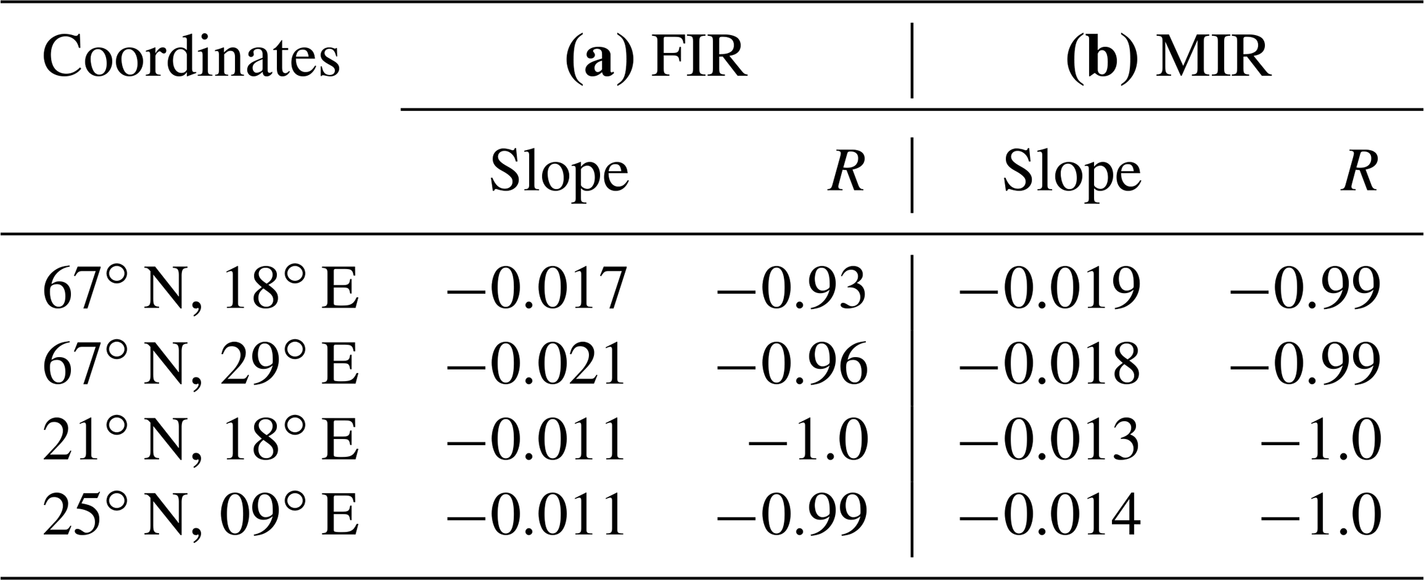
The following three points can be highlighted from these results:

• With the exception of 67^∘ N, 29^∘ E, the slope of the linear fit is steeper in the MIR than in the FIR.

• In both spectral regions, the slope of 67^∘ N, 18^∘ E and 67^∘ N, 29^∘ E is steeper than that of the other two scenes.

• For scenes 67^∘ N, 18^∘ E; 67^∘ N, 29^∘ E; and 25^∘ N, 09^∘ E, the scatter of values is larger in the FIR than the MIR (lower R in Table C1).

A possible cause for the variation in slopes can be found in the form of B(T_s). To see this let L_d=0, which primarily simplifies the analysis but is also a valid assumption for the MIR and for the centres of the FIR microwindows. Equation (3) then becomes the following:

$$\begin{array}{}\text{(C2)}& S_{\text{surf}}=\mathit{ϵ}B\left(T_{\text{s}}\right),\end{array}$$

where the σ underscore has been dropped for convenience. Keeping S_surf constant, the equation is rearranged to get an expression for ϵ and then the derivative is taken with respect to T_s as follows:

$$\begin{array}{}\text{(C3)}& \begin{array}{rl}{\displaystyle \frac{\text{d}\mathit{ϵ}}{\text{d}{T}_{\text{s}}}}& ={\left.S_{\text{surf}}{\displaystyle \frac{\mathrm{1}}{-B^{\mathrm{2}}\left(T_{\text{s}}\right)}}{\displaystyle \frac{\text{d}B\left(T\right)}{\text{d}T}}\right|}_{T_{\text{s}}}\\ & =-\mathit{ϵ}\left[{\left.{\displaystyle \frac{\mathrm{1}}{B\left(T_{\text{s}}\right)}}{\displaystyle \frac{\text{d}B\left(T\right)}{\text{d}T}}\right|}_{T_{\text{s}}}\right].\end{array}\end{array}$$

The dominating factor in determining $\text{d}\mathit{ϵ}/\text{d}{T}_{\text{s}}$ (the slope in Fig. C1a and b) for a given scene and wavenumber is the expression in brackets on the right-hand side of Eq. (C3), as although ϵ also varies spectrally and geographically, its average variations are an order of magnitude smaller (20 % as opposed to 800 %). The plot in Fig. C1c shows this expression for the surface temperatures of the four different scenes. This plot shows that the value of this expression increases with wavenumber and is lower for higher T_s. This behaviour could explain the difference in slopes observed in Fig. C1a and b. The larger value of this term and, thus, $\text{d}\mathit{ϵ}/\text{d}{T}_{\text{s}}$ in the MIR would result in the steeper slope observed for most scenes in the MIR. And as 67^∘ N, 18^∘ E and 67^∘ N, 29^∘ E are much colder scenes, it is expected that the slope of their linear relation will be steeper than that of 21^∘ N, 18^∘ E and 25^∘ N, 09^∘ E.

Finally, an analytic correlation analysis can shed light on the scatter about the linear trend of the values in Fig. C1​​​​​​​a and b (also represented by the size of their R correlation value in Table C1). In Fig. C1d, the analytic Pearson correlation coefficient of the retrieval uncertainties of T_s and emissivity is shown. The uncertainties are given in the retrieval uncertainty covariance matrix S_x defined in Eq. (4). Using the standard formula for the analytic (population) Pearson correlation coefficient, as follows:

$$\begin{array}{}\text{(C4)}& \text{Corr}(T_{\text{s}},{\mathit{ϵ}}_i)={\displaystyle \frac{\text{Cov}(T_{\text{s}},{\mathit{ϵ}}_i)}{{\mathit{\sigma }}_{T_{\text{s}}}{\mathit{\sigma }}_{{\mathit{ϵ}}_i}}}={\displaystyle \frac{{\mathbf{S}}_{T_{\text{s}},{\mathit{ϵ}}_i}}{\sqrt{{\mathbf{S}}_{T_{\text{s}},T_{\text{s}}}}\sqrt{{\mathbf{S}}_{{\mathit{ϵ}}_i,{\mathit{ϵ}}_i}}}},\end{array}$$

where ${\mathbf{S}}_{T_{\text{s}},T_{\text{s}}}={\mathit{\sigma }}_{T_{\text{s}}}$ is the retrieval uncertainty standard deviation of T_s (dropping the x in S for visibility), and similarly for ϵ_i, the ith value in the emissivity retrieval vector. Note that Fig. C1d only shows this value for the baseline retrieval of the four scenes and is thus meant as an illustration of the spectral structure of the correlation and not as a quantitative reference.

Figure C1d shows that, as expected T_s, and emissivity are not correlated to the same extent in different spectral regions. The correlation mirrors the spectral structure seen in the emissivity Jacobian (see Fig. 3). Unsurprisingly, as it is calculated from S_x, which in turn is calculated from the Jacobian (and from S_a). There is a strong uniform correlation of the MIR emissivity points with T_s, while the correlation of the FIR values depends on the microwindow structure and, with that, on the dryness of the atmosphere. The ∼ 750–1250 cm⁻¹ region of the MIR is called the atmospheric window as it is almost fully transparent to the surface, and thus, in most of that region, the strength of the correlation is determined solely by the value of the surface temperature. In the FIR, the difference in correlation strength is harder to attribute precisely, as it is due to a combination of the pwv and the surface temperature. However, its value for the four scenes analysed here can still be used to compare the correlation to the scatter seen in Fig. C1a and b. These show good agreement, as the scenes with a lower retrieval uncertainty correlation coefficient also have a smaller systematic uncertainty correlation and larger scatter around the linear trend.

In summary, the correlation of surface temperature and emissivity behaves as would be expected from the physics of the forward model. The range of systematic uncertainties in Fig. C1a and b confirm what was already shown in Sect. 6.2 and 6.1, namely that this correlation allows for a range of retrieved emissivities depending on the retrieval parameters. The predictability of the behaviour of the correlation is important for the evaluation of this effect, which should be thoroughly quantified during the development of the operational retrieval.