the Creative Commons Attribution 4.0 License.
the Creative Commons Attribution 4.0 License.
 | 24 Mar 2022
Time evolution of temperature profiles retrieved from 13 years of infrared atmospheric sounding interferometer (IASI) data using an artificial neural network
Marie Bouillon
Sarah Safieddine
Simon Whitburn
Lieven Clarisse
Filipe Aires
Victor Pellet
Olivier Lezeaux
Noëlle A. Scott
Marie Doutriaux-Boucher
Cathy Clerbaux
The three infrared atmospheric sounding interferometers (IASIs), launched in 2006, 2012, and 2018, are key instruments to weather forecasting, and most meteorological centres assimilate IASI nadir radiance data into atmospheric models to feed their forecasts. The European Organisation for the Exploitation of Meteorological Satellites (EUMETSAT) recently released a reprocessed homogeneous radiance record for the whole IASI observation period, from which 13 years (2008–2020) of temperature profiles can be obtained. In this work, atmospheric temperatures at different altitudes are retrieved from IASI radiances measured in the carbon dioxide absorption bands (654–800 and 2250–2400 cm−1) by selecting the channels that are the most sensitive to the temperature at different altitudes. We rely on an artificial neural network (ANN) to retrieve atmospheric temperatures from a selected set of IASI radiances. We trained the ANN with IASI radiances as input and the European Centre for Medium-Range Weather Forecasts (ECMWF) reanalysis version 5 (ERA5) as output. The retrieved temperatures were validated with ERA5, with in situ radiosonde temperatures from the Analysed RadioSoundings Archive (ARSA) network and with EUMETSAT temperatures retrieved from IASI radiances using a different method. Between 750 and 7 hPa, where IASI is most sensitive to temperature, a good agreement is observed between the three datasets: the differences between IASI on one hand and ERA5, ARSA, or EUMETSAT on the other hand are usually less than 0.5 K at these altitudes. At 2 hPa, as the IASI sensitivity decreases, we found differences up to 2 K between IASI and the three validation datasets. We then computed atmospheric temperature linear trends from atmospheric temperatures between 750 and 2 hPa. We found that in the past 13 years, there is a general warming trend of the troposphere that is more important at the poles and at mid-latitudes (0.5 K/decade at mid-latitudes, 1 K/decade at the North Pole). The stratosphere is globally cooling on average, except at the South Pole as a result of the ozone layer recovery and a sudden stratospheric warming in 2019. The cooling is most pronounced in the equatorial upper stratosphere (−1 K/decade). This work shows that ANN can be a powerful and simple tool to retrieve IASI temperatures at different altitudes in the upper troposphere and in the stratosphere, allowing us to construct a homogeneous and consistent temperature data record adapted to trend analysis.
- Article
(4049 KB) - Full-text XML
-
Supplement
(587 KB) - BibTeX
- EndNote


Atmospheric temperatures are a key component of Earth's climate. In the past few decades, a warming of the troposphere due to the increase in greenhouse gas concentrations (Tett et al., 2002; Santer et al., 2017; Susskind et al., 2019; Masson-Delmotte et al., 2022) and a cooling of the stratosphere have been observed (Randel et al., 2016; Maycock et al., 2018). Stratospheric temperatures are impacted by both anthropogenic forcing (e.g. greenhouse gas emissions, ozone depletion) and natural forcing (e.g. volcanic eruptions, solar cycle) (Aquila et al., 2016). The study of stratospheric temperatures and their long-term evolution is therefore critical to understand the roles of these different forcings on the evolution of climate in the stratosphere, but also in the troposphere.
Long-term atmospheric temperature records can be obtained from in situ measurements (lidars and radio soundings). These observations are generally of excellent quality; however, they are sparse and unevenly distributed around the globe. More recently, satellite-derived temperatures have become a key component for climate change monitoring (Li et al., 2011; Yang et al., 2013). Satellite observations have a better spatial coverage, but the construction of a long temperature record from these observations usually requires merging several different instruments, and corrections and adjustments between the observations are needed to obtain a homogeneous dataset (Zou et al., 2014; Seidel et al., 2009).
In 2006, the first infrared atmospheric sounding interferometer (IASI) was launched on the Metop satellite. IASI measures radiance spectra from which surface and atmospheric temperatures (Hilton et al., 2012; Safieddine et al., 2020a) and trace gas concentrations can be retrieved (Clerbaux et al., 2009; Clarisse et al., 2011). A second instrument and then a third were launched in 2012 and 2018, and the comparison between the three instruments has shown excellent agreement (Boynard et al., 2018; EUMETSAT, 2013a). Since IASI is planned to fly for at least 18 years, with the three instruments built at the same time and flying in constellation, continuity and stability are ensured, and the construction of a long-term climate data record at a range of altitudes is becoming possible.
IASI radiance spectra and derived atmospheric temperature profiles are routinely processed by the European Organisation for the Exploitation of Meteorological Satellites (EUMETSAT). Over the past 13 years, EUMETSAT has performed several updates on the real-time processing of both radiances and temperatures, making the time series non-homogeneous. The impacts of these updates have been evidenced in several studies (George et al., 2015; Van Damme et al., 2017; Parracho et al., 2021) and quantified in Bouillon et al. (2020). For temperatures, the “jumps” in the time series due to these updates make them unfit for the computation of trends. In 2018, EUMETSAT reprocessed the Metop-A radiance dataset (https://doi.org/10.15770/EUM_SEC_CLM_0014; EUMETSAT, 2018), providing a new radiance dataset over time. After 2018, the radiances are stable and consistent with those reprocessed (Bouillon et al., 2020).
In this work, we present a new atmospheric temperature product derived from the homogeneous IASI radiance dataset, using an artificial neural network (ANN) technique, to derive a homogeneous temperature data record. In Sect. 2, we present the data used in this study, and in Sect. 3, we explain the method used to compute the temperatures, which consists of selecting the appropriate IASI channels and training the ANN. In Sect. 4, we compare the outputs of the neural network with both the latest ECMWF reanalysis (ERA5) and Analysed RadioSoundings Archive (ARSA) radiosonde temperatures to validate the new data. In Sect. 5 we compute atmospheric temperature trends for the past 13 years. Conclusions are listed in Sect. 6.
2.1 IASI radiances
Each of the three IASI instruments are mounted on board the Metop platform flying in a polar orbit at an altitude of 817 km. The IASI swath contains 30 fields of view with 4 pixels in each field of view. This observation mode allows each IASI instrument to observe the entire Earth twice a day, between 09:15 and 09:45 as well as between 21:15 and 21:45 local time. IASI measures the radiation of the Earth–atmosphere system in the thermal infrared in 8461 channels between 645 and 2760 cm−1 (resolution of 0.25 cm−1, 0.5 cm−1 apodized; Clerbaux et al., 2009).
2.2 ERA5 reanalysis
The European Centre for Medium-Range Weather Forecasts (ECMWF) reanalysis (ERA5; Hersbach et al., 2018; Copernicus Climate Change Services, 2019) is a 4D-Var data assimilation product. It is part of the Integrated Forecast System (IFS) that provides variables relevant to the atmosphere, land, and ocean (ECMWF, 2016). The ERA5 atmospheric temperature product used in this work is hourly and is available on 37 pressure levels (from the surface up to 0.01 hPa). ERA5 actually assimilates IASI radiances from Metop-A and Metop-B as well as high-spectral-resolution radiances from other instruments such as the Atmospheric InfraRed Sounder (AIRS) on Aqua and the cross-track infrared sensor from the Suomi National Polar-orbiting Partnership and the National Oceanic and Atmospheric Administration. Note that IASI is the largest contributor to error reduction for global numerical weather prediction in the thermal infrared spectral band (Borman et al., 2016).
2.3 Analysed RadioSoundings Archive
The Analysed RadioSoundings Archive (ARSA) is a 41-year (1979–2019) database of radiosonde temperature profile measurements from different stations around the globe (Scott et al., 2015). ARSA provides 43 pressure level profiles (from the surface to 0.0026 hPa) of temperature, water vapour and ozone, and surface temperature. The raw radiosonde observations go through severe multistep quality controls to eliminate gross errors. If the selected radiosonde measurement is unable to provide forward radiative transfer modellers with the required information (above 30 hPa for temperature), ARSA combines existing radiosonde measurements with other reliable data sources to complete the description of the atmospheric state as high as 0.0026 hPa. Temperature profiles are thus extrapolated with ERA-Interim (Dee et al., 2011) outputs between 30 and 0.1 hPa for temperature. Above 0.1 hPa, the profiles are extrapolated up to 0.0026 hPa using a climatology of Atmospheric Chemistry Experiment – Fourier Transform Spectrometer (ACE-FTS) Level 2 from SCISAT. ARSA was validated against IASI observations by simulating spectra from the Automatized Atmospheric Absorption Atlas (4A/OP) forward model (Scott and Chédin, 1981) with ARSA profiles as inputs and comparing them with space-time-collocated IASI observations. The pertinence of the requested modifications after this validation has also been assessed against the TIROS Operational Vertical Sounder (TOVS), the Advanced TIROS Operational Vertical Sounder (ATOVS; Reale et al., 2008), AIRS (Lambrigtsen et al., 2004), the High resolution Infrared Radiation Sounder (HIRS/4; EUMETSAT, 2013b), and the Microwave Humidity Sounder (MHS; Hans et al., 2020). Based on these validations, incorrect or unreliable data inherent to the quality of the radiosondes were completed using measurement data of other relevant auxiliary datasets (in particular Level 2 results of ACE-FTS temperature profiles above 10 hPa). It is useful to recall that ARSA is being reprocessed to replace ERA-Interim with ERA5. This will allow, among other things, the period to be extended beyond summer 2019, when the production of ERA-Interim stopped.
2.4 EUMETSAT CDR of all-sky temperature profiles
In 2020, EUMETSAT released a climate data record (CDR) of all-sky IASI temperature (https://doi.org/10.15770/EUM_SEC_CLM_0027), so the temperature is homogeneous over the whole IASI time series (EUMETSAT, 2020). The reprocessed temperatures were computed with a piecewise linear regression cube (PWLR3) algorithm, using all IASI observations in input (clear and cloudy scenes) and observations from two other microwave instruments flying on board the Metop-A and Metop-B satellites: the Microwave Humidity Sounding (MHS) and the Advanced Microwave Sounding Unit (AMSU-A).
The basic principle of this algorithm is a linear regression between IASI radiance observations and real atmospheric temperatures. To take into account the non-linearity between the observations and the temperatures, the training dataset is divided into several sub-datasets, resulting from a k-means clustering. This ensures that, in each sub-dataset, a linear relationship is a good approximation between the observations and the temperature, and different linear regression coefficients are computed for each sub-dataset.
3.1 The IASI instrument channel selection
Using the 8461 channels of IASI raises practical issues for storage and computation power as retrieval and assimilation algorithms can hardly handle such a large amount of information. A channel selection is usually needed when dealing with IASI (Rabier et al., 2002; Collard, 2007; Pellet and Aires, 2018). To retrieve atmospheric temperatures, we select IASI channels that are most sensitive to the temperature profile. Most of the channels selected are located in the carbon dioxide (CO2) absorption band because the radiances observed in these channels are more sensitive to atmospheric temperature than CO2 concentrations (Chédin et al., 2003; Collard, 2007). The selection is obtained using the entropy reduction (ER) method (Rodgers, 2000). The entropy describes the probabilities of all the possible states, and it is maximal when all the states have an equal probability. Selecting the channels that reduce the most the entropy means selecting the channels that bring the most information about the state. ER is computed using
where B is the a priori covariance matrix, and A is the retrieval covariance matrix, described in Eq. (2):
where H is the matrix of the temperature-weighting functions (the sensitivity of the IASI brightness temperature to the temperature), and R is the instrumental noise plus the radiative transfer error.
With A, it is possible to compute the entropy reduction in each channel as follows:
with h′ being the Jacobian of the considered channel normalized by the noise (H′ = H). For the selection of the first channel, we set A0 = B. With this, we selected the channel with the largest entropy reduction, and the theoretical covariance matrix is updated as follows:
We then repeat this process until the chosen number of channels has been selected or until the entropy has been reduced enough. This method has been used to retrieve land surface temperature from IASI (Safieddine et al., 2020a), and we apply it here for atmospheric temperature profiles.
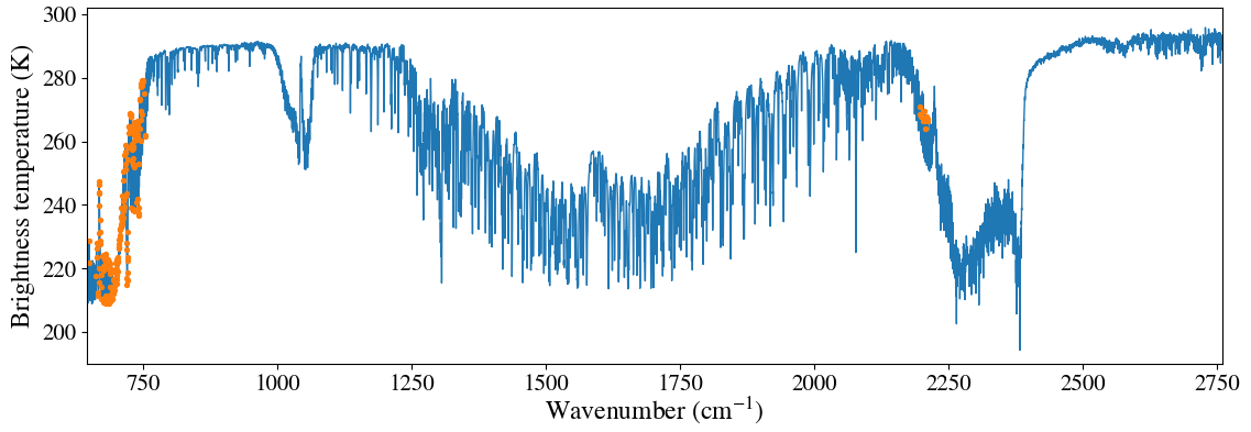
Figure 1IASI clear-sky spectrum in brightness temperature in kelvin (blue), with the selected channels in orange.
To take into account the effect of the different parameters affecting the selection, two experiments were conducted: in the first, we considered 200 channels. The channels were selected while taking into account the perturbation of the radiances due to water vapour (H2O) and ozone (O3) variations because some channels are sensitive to temperature, H2O, and O3 (Pellet and Aires, 2018). The uncertainty in the state of unretrieved species (i.e H2O and O3) impacts the potential retrieval of the temperature using these channels. This perturbation is then computed with (with x being the variable considered: H2O or O3) and is added to the instrumental noise and radiative transfer error, so A becomes
The second experiment consists of 100 channels. Before the ER method is applied to all the channels, the channels for which the variability in atmospheric gases (H2O, O3, CO and CH4) and emissivity has an impact higher than 30 % of the instrumental noise are removed.
In the first selection, the weighting functions were computed with the Optimal Spectral Sampling (OSS) radiative transfer model (Moncet et al., 2015). In the second selection, the model used was Radiative Transfer for TOVS (RTTOV; Saunders et al., 2018).
For each of the two selection methods, the number of channels selected is increased until adding more new channels does not significantly improve the results.
The goal of using these two sets of experiments is to choose from these two the best and most sensitive channels to different atmospheric temperatures while taking into account the different atmospheric perturbations and errors that might affect the selection. On its own, each experiment was tested (not shown here), and the best result was achieved when combining them both.
For the computation of temperatures, we used a mix of the two experiments, consisting of 231 channels (with 69 channels in common between the two). Figure 1 shows the selected channels on a typical IASI spectrum. Most of the channels are in the carbon dioxide (CO2) absorption band between 645 and 800 cm−1, while a few (14 channels) are at 2200 cm−1 in the N2O absorption band. The full list of the channels is provided in the Supplement (Table S1).
3.2 Artificial neural network
We trained a two-layer artificial neural network (ANN) to estimate atmospheric temperature profiles. This method has been used for instance in Aires et al. (2002), using IASI-simulated radiances before its launch.
A total of 450 000 IASI observations are used to train the ANN. These observations (3000 scenes per month) were selected randomly around the globe between January 2008 and December 2020. This training dataset is composed of day and night and clear- and cloudy-sky observations mixed together. The input data consist of the pseudo-normalized radiances (multiplied by 104 so that their order of magnitude is not too small compared to temperatures) in the selected channels as well as the scan angle of the observation. A monthly value for global CO2 concentration was also added to take into account the CO2 variations that affect the radiance values measured in the selected channels. The CO2 monthly values come from the NOAA Earth System Research Laboratories global monitoring dataset (https://gml.noaa.gov/ccgg/trends/, last access: 15 December 2021; Dlugokencky and Tans, 2021). As the expected output of the training of the ANN, we use the ERA5 temperatures interpolated to the latitudes, longitudes, and time of the IASI observations. These temperatures are given on a static pressure level grid. We chose ERA5 because it is the most complete homogeneous dataset of temperatures available, allowing us to select observations in any year and any type of sky. A set of 50 000 different observations (selected the same way as the 450 000) is used to assess the quality of the ANN at the end of the training.
The temperatures are computed at 11 fixed pressure levels: 2, 7, 10, 20, 30, 70, 100, 200, 400, 550, and 750 hPa. These were chosen based on the weighting functions of the 231 selected channels, shown in Fig. 2. The weighting functions show the sensitivity of IASI channels to the temperature profile in K K−1. The weighting functions do not change significantly under day or night conditions, and this does not have an impact on the retrieval. We see in Fig. 2 that the weighting functions peak at different altitudes, in particular for pressures larger than 10 hPa, suggesting that IASI has a good information content at these altitudes. The pressure levels were chosen based on a tradeoff between having equally distributed levels along the vertical while matching the maxima of the weighting functions of the selected channels. The pressure levels are shown by dashed horizontal lines in Fig. 2. At the selected pressure levels, the vertical resolution goes from 5 to 12 km from the lower to the upper troposphere. In the stratosphere, the resolution goes from 12 km in the lower stratosphere to 25 km above 7 hPa. We tried different configurations for the ANN, changing the number of epochs for the training and the number of neurons in the two hidden layers. The configuration giving the best results is 5000 epochs and 150 neurons in the two hidden layers. As a result, we have an ANN with 233 neurons in the input layer (231 radiance values, 1 scan angle, and 1 CO2 value), 150 neurons in each of the two hidden layers, and 11 neurons in the output layer (the 11 pressure levels shown by horizontal lines in Fig. 2).
We used the trained ANN to retrieve temperatures from all IASI observations between 2008 and 2020. After the temperature profiles are computed, we use a static filter based on ERA5 mean surface pressure between 2008 and 2020 to account for orography (as some high-altitude regions do not have temperature at 750 hPa for instance).
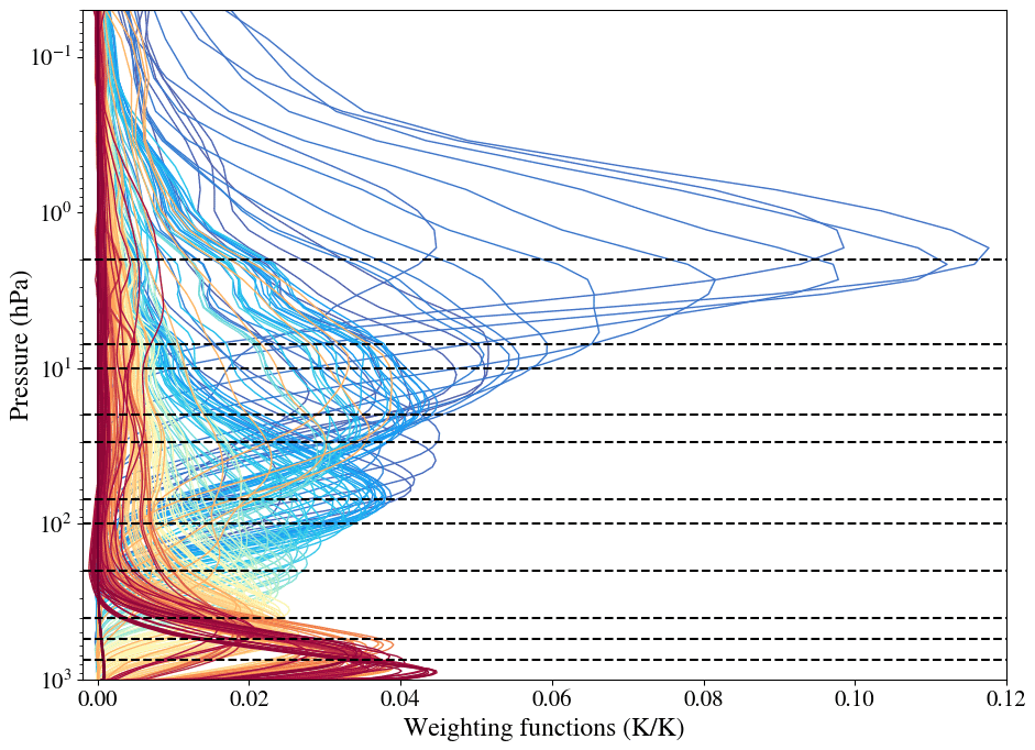
Figure 2Weighting functions for the 231 selected IASI channels. Dashed horizontal lines represent the 11 pressure levels for which the temperatures are computed. The colours of the weighting functions represent the wavenumbers of the selected channels (blue for the channels around 700 cm−1, red for the channels around 2200 cm−1).
Atmospheric temperatures between 2008 and 2020 were computed at the 11 pressure levels. We use Metop-A observations until 2017 and Metop-B observations for 2018 onwards. The Metop-A satellite was exploited in a drifting orbit from June 2017 in order to extend its lifetime to the end of 2021 (EUMETSAT, 2017). We compare the whole IASI time series with the temperatures from ERA5 reanalysis, from ARSA, and from the EUMETSAT CDR.
4.1 Comparison with ERA5
Although the neural network was trained with ERA5, it does not reproduce the same temperatures. The output of the retrieval is mainly governed by the variations in observed radiances, and ERA5 can be used for validation.
ERA5 temperatures are given on a latitude–longitude grid. For the comparison with the IASI-ANN output, ERA5 temperatures were interpolated to the time, latitudes, and longitudes of IASI observations. We then computed the daily zonal mean of the IASI-based ANN temperatures and ERA5 and looked at the differences between the two datasets. Figure 3 illustrates the zonal mean differences between the ANN retrievals and ERA5 from 2008 to 2020 for the 11 pressure levels considered in this study and the time-averaged differences.

Figure 3Daily zonal mean differences between IASI and ERA5 zonal mean temperature for the 11 pressure levels of the ANN, with the time-averaged differences on the right of each subplot.
Between 200 and 750 hPa, the differences are less than 0.5 K at all latitudes. We see slight seasonal variations in the differences at 200, 400, and 550 hPa. At 750 hPa, the seasonal variations are more pronounced and more often negative than at the other pressure levels. Note that due to orography at this pressure level, there are no data over the South Pole, Greenland, and in the major mountain ranges.
Between 7 and 100 hPa, the differences between the two datasets are less than 0.5 K at mid-latitudes and at the poles. Around the Equator (30∘ S to 30∘ N), the differences are slightly larger (1 K). Figure 4 shows the monthly mean of the differences between 10∘ S and 10∘ N from 100 to 7 hPa as well as the monthly zonal wind from ERA5 in the same latitude range. Positive differences (ANN temperatures larger than ERA5) are correlated to negative zonal wind, and negative differences are correlated to positive zonal wind. This suggests that the neural network overestimates temperatures during the easterly phase of the quasi-biennial oscillation (QBO).
At 2 hPa, the differences range from −2 to 2 K globally. This is because the IASI channel selection is less sensitive to temperature changes at these pressure levels. In Fig. 2, we see that the channels peaking at this pressure level have high sensitivity, but there are fewer of them compared to other pressure levels.
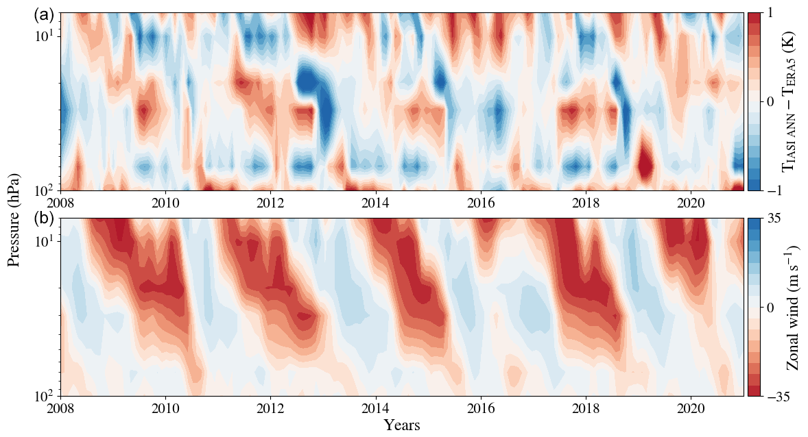
Figure 4Monthly mean of the temperature differences between IASI-ANN and ERA5 (a) and monthly zonal wind from ERA5 (b) between 10∘ S and 10∘ N.

Figure 5Root mean square of the daily differences between IASI retrievals and ERA5 on a 1∘ × 1∘ latitude–longitude grid over the period 2008–2020.
When taking day and night observations separately (not shown), there is no significant change in the differences.
Since averaging the differences over longitudes makes them smaller, we looked at the daily spatial differences. We gridded the ANN retrievals and ERA5 (interpolated to IASI coordinates) on a latitude–longitude grid and computed the root mean square (rms) of the daily differences in each of the bins of the grid and at each pressure level. Figure 5 shows the rms of the daily differences for the 2008–2020 period.
At 750 hPa, rms values are about 0.5 K at the Equator and larger at higher latitudes (between 1 and 2 K), especially around mountain ranges, where they reach 3 K and can be due to gravity wave activity. Between 550 and 200 hPa, the rms values are of 0.5 K almost everywhere. There are regions (in particular the Antarctica, Greenland, and the Himalaya at 550 hPa) where the rms can reach 2 K. Between 100 and 7 hPa, the rms values are small at high latitude (0.5 K) and large at the Equator (between 1.5 and 2 K). At 7 and 10 hPa, the band at the Equator with larger rms reaches higher latitudes (about 50∘ N and S). The large rms values correspond to the high differences seen at the Equator in Fig. 3. At 2 hPa, the rms values are between 2 and 3 K everywhere, which is consistent with Fig. 3.
4.2 Comparison with ARSA
For the comparison with our IASI retrievals, we interpolated ARSA temperature profiles to the 11 pressure levels of the ANN, and we only kept the stations for which there were at least 300 observations per year between 2008 and 2018. Figure 6 shows the positions of these stations.
We then added the 14 stations present in Antarctica and the 6 stations in Greenland to have observations at high latitudes, although these stations have fewer than 300 observations per year. The stations in Greenland have between 150 and 300 observations per year on average, so the time coverage is still satisfactory. However, in Antarctica, the stations have between 10 and 150 observations per year, and only two stations have more than 100 observations per year.

Figure 6Locations of the ARSA stations with at least 300 observations per year (crosses) and the stations in two other regions (Greenland and Antarctica) that do not satisfy this condition are marked with triangles. The rectangles of colour correspond to the regions in which we compared IASI temperatures to ARSA.
We divided the stations into eight distinct regions, and we computed the daily mean temperature of all the observations of each region. We interpolated IASI temperatures to the latitude, longitude, and time of each considered station, and we computed the daily mean IASI temperature in each region. We then computed the differences between the two datasets.
Figure 7 shows the daily differences between IASI retrievals and ARSA mean regional temperature in the eight selected regions between 2008 and 2018 and the time-averaged difference profiles. We only show differences between 750 and 30 hPa as ARSA data above 30 hPa do not always come from radiosounding measurement but from the extrapolation datasets. Between 7 and 100 hPa, the differences are small and mostly negative (about 0.5 K). At 200 hPa and below, the differences remain small and negative in the Pacific, Oceania, and East Asia. In Greenland, North America, and Europe, the differences at these pressure levels are slightly larger and more often positive (about 0.5 K, up to 1 K in North America and Europe) than in the other regions.

Figure 7Daily differences between IASI-ANN and ARSA temperatures between 2008 and 2018 in North America, Europe, the Arabian Peninsula, East Asia, Oceania, the Pacific, Greenland, and Antarctica, with the time average difference profiles on the right of each subplot.
In Antarctica and, to a lesser extent, the Arabian Peninsula, there are more daily variations in positive and negative differences, and they are a little larger (about 0.7 K in the Arabian Peninsula and 1 K in Antarctica) than in the other regions. This can be because of the low space (few stations) and time coverage (only for Antarctica) in these regions. However, we see the same pattern as in the other regions: large differences at 2 hPa; small differences at 7 hPa; and lower, more positive differences in the troposphere.
In all the regions, the time-averaged differences range from −0.6 to 0.6 K except in the Arabian Peninsula at 750 hPa, where they reach 0.9 K.
Figure S1 shows the differences between ERA5 and ARSA over the same period and in the same regions, with ERA5 interpolated to the latitudes, longitudes, and time of the ARSA observations. The differences between ERA5 and ARSA are very similar to those between IASI retrievals and ARSA, but slightly smaller (less than 0.3 K between 750 and 7 hPa). Figure S2 shows the differences between IASI and ERA5 temperatures interpolated to the time and locations of ARSA observations. In most regions, the differences are less than 0.5 K. In Antarctica, in Europe (troposphere only), and in the Arabian Peninsula and Oceania (stratosphere only), the differences can reach 1 K.
Figure 8 shows the standard deviation of the daily differences between IASI-ANN and ARSA temperatures and the correlation between the two datasets in the eight regions. In most regions, the standard deviation ranges from 0.5 to 1 K, except in the Arabian Peninsula and East Asia, where they reach 1.3 K at 750 hPa, and in Antarctica and Europe, where they range from 1 to 2 K. The correlations between IASI-ANN and ARSA temperatures show that there is no significant bias between the two datasets.
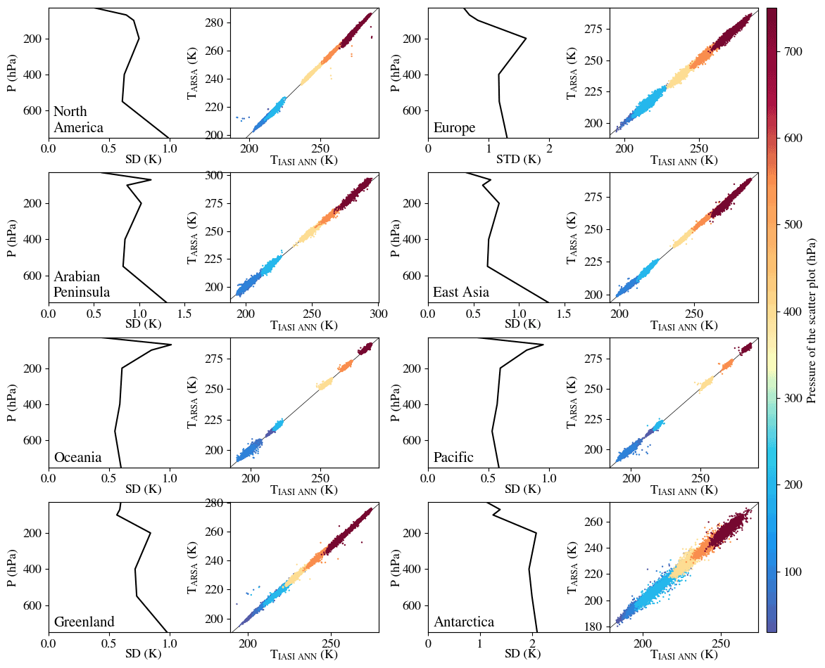
Figure 8Standard deviation profiles of the differences between IASI-ANN and ARSA temperatures (left of each subplot) and correlation between the two datasets (right of each subplot).
Figures 3, 5, 7, and 8 show that between 7 and 750 hPa, the IASI-ANN product can be considered to be good-quality temperatures, very consistent with the temperatures of the ERA5 and ARSA datasets (differences smaller than 1 K at most latitudes, 2 K at the Equator). At 2 hPa, the quality of the ANN product decreases as it was reflected in the lower count of weighting functions of IASI (Fig. 2). This means that at 2 hPa, the temperatures are not accurate enough to follow the long-term evolution of atmospheric temperatures. However, they can still be used to study large variations in temperature (during extreme events for example).
4.3 Comparison with the EUMETSAT reprocessed temperature record
We compared the ANN retrievals with this reprocessed EUMETSAT CDR. Since the two methods use the same IASI observation input, there is no need for an interpolation over the coordinates of the observations. However, EUMETSAT temperature profiles are retrieved on 138 levels, reflecting the 137 hybrid levels from the ERA-5 L137 grid plus the surface level, so we interpolated EUMETSAT temperatures to the fixed pressure levels of the ANN. Figure 9 shows the differences between the zonal mean temperatures of the ANN output and EUMETSAT.
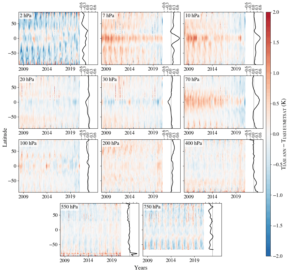
Figure 9Daily zonal mean differences between IASI-ANN output and IASI EUMETSAT zonal mean temperature for the 11 pressure levels of the ANN. The red stripes seen in some panels are artefacts from the analysis, and they do not reflect a physical phenomenon.
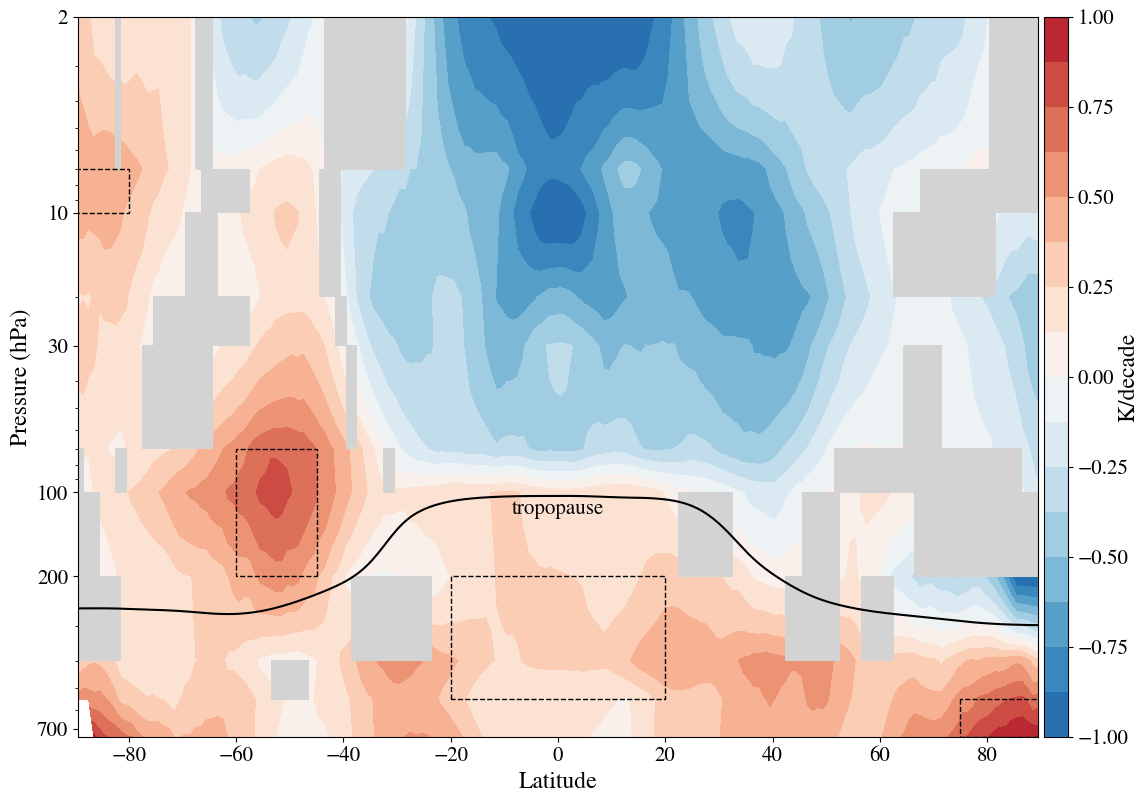
Figure 10Zonal temperature trends for the period 2008–2020 computed with the outputs of the ANN. Grey areas correspond to trends that are not statistically significant. The dotted rectangles represent the regions for which the time series are shown in Fig. 11.
The differences are small at all pressure levels (less than 0.5 K), except at 2 hPa, where they can reach 1 K, and we see seasonal variations in the differences that are more pronounced in the troposphere (750, 550, and 400 hPa). At 7, 10, and 70 hPa, the differences are positive and larger at the Equator, and they decrease over time. This bias can also be seen at higher latitudes and other pressure levels, although it is less obvious. This bias might be due to the fact that EUMETSAT's algorithm does not use CO2 in input, and the retrieval is impacted by the variations in the CO2 over time, which we account for.
Note that although the ANN and EUMETSAT retrievals are both based on IASI radiances, the two temperature records are not redundant. The two datasets use different observations (IASI radiances and CO2 concentrations for the ANN and IASI, AMSU, and MHS radiances for EUMETSAT) and different methods of retrieval (ANN and PWLR3). When needed, our dataset can constantly be enhanced and rapidly reprocessed for the entire time series. EUMETSAT CDR can be produced for every major change in the operational real-time all-sky temperature processor.
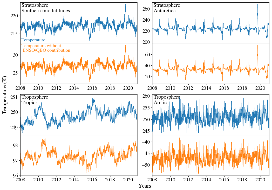
Figure 11Time series of temperatures in the four rectangles of Fig. 10 (blue) and time series without ENSO and QBO contributions (orange). The exact locations of the four regions are 45–60∘ S and 100–70 hPa for southern-stratosphere mid-latitudes, 80–90∘ S and 10–7 hPa for the Antarctic stratosphere, 20∘ S–20∘ N and 550–200 hPa for the tropical troposphere, and 75–90∘ N and 750–550 hPa for the Arctic troposphere.
We used the ANN temperatures to compute trends over the past 13 years. One of IASI's main assets is its high radiometric stability over the years, and it is used as a reference for the inter-calibration of infrared sensors by the Global Space-based Inter-Calibration System (Golberg et al., 2011), so temperatures derived from IASI radiances are a good product to study atmospheric trends.
We use IASI daily zonal mean temperature (latitude bands of 1∘), and we compute the Theil–Sen estimator for each latitude and each pressure level. The Theil–Sen estimator is a robust method for computing linear trends, where the trend is determined by the median of all the possible slopes between pairs of points (Theil, 1950; Sen, 1968). We also computed the associated p values, with a 0.05 threshold for significance being considered. Before the Theil–Sen estimator was applied, we removed the contributions of El Niño–Southern Oscillation (ENSO) and the QBO to temperatures. Their contribution was computed using a multiple linear regression based on the multivariate ENSO index (MEI; https://psl.noaa.gov/enso/mei/, last access: 10 January 2022; NOAA, 2022a) and the QBO30 and QBO50 indices (equatorial zonal winds at 30 and 50 hPa; https://www.cpc.ncep.noaa.gov/data/indices/, last access: 10 January 2022; NOAA, 2022b). Figure 10 shows the significant temperature trends for the 2008–2020 period. Non-significant trends are shown in grey in Fig. 10.
We clearly see a warming in the troposphere. In the tropics, we see a warming of 0.2–0.3 K/decade. At mid-latitudes, the warming is stronger (0.5–0.6 K/decade). As highlighted by previous studies (Masson-Delmotte et al., 2022), the poles are where tropospheric temperatures are warming the quickest, especially the Arctic, where temperatures increase by 1 K/decade (Arctic amplification). The values of the trends we found between 45∘ S and 45∘ N are similar to those found by Shangguan et al. (2019).
In the stratosphere, we observe a cooling at all latitudes north of 40∘ S. The cooling is strongest at the Equator, above 20 hPa (−1 K/decade). In the Arctic, there is no significant trend. This cooling of the stratosphere has also been observed by Maycock et al. (2018) and Randel et al. (2016), although their values are smaller than those found here (but their time period is also different). In the Southern Hemisphere, we see two areas of warming: a strong one at 50∘ S and 100 hPa (1 K/decade) and another located at 80∘ S and 10 hPa (0.4 K/decade). Part of this warming is due to a sudden stratospheric warming (SSW) that happened in September 2019 (Safieddine et al., 2020b). The temperature increased by more than 30 K in a few days. Such a warming toward the end of our study period has a strong impact on trends. However, the computation of trends over the period 2008–2018 still shows warming in these two regions, and it cannot all be attributed to the SSW. The warming is weaker at 50∘ S, 100 hPa (0.6 K/decade) and stronger at 80∘ S, 10 hPa (0.8 K/decade). Due to the Montreal Protocol in 1987, the ozone hole has been recovering since the 1990s (WMO, 2018; Weber et al., 2018; Strahan et al., 2019), and warming in the stratospheric South Pole can partly be attributed to this recovery.
Figure 11 shows the temperature time series in the regions delimited by dashed rectangles in Fig. 10. The time series are shown with and without the contributions of ENSO and QBO. In the equatorial troposphere, we see that temperatures are increasing. However, removing the contribution of ENSO significantly reduces the warming trend as most of it was driven by the strong El Niño event of 2015–2016. In the Arctic troposphere, there are no significant differences in the time series with and without the contribution of ENSO and QBO, suggesting that these phenomena do not have a large impact on Arctic temperature, and the warming observed in this region is due to the increase in greenhouse gases and Arctic amplification. In the southern stratosphere, the trend in both warming regions seems to be driven by the 2019 SSW. However, we see a continuous increase in temperatures before 2019 (with and without ENSO and QBO contribution) that cannot be attributed to the SSW and is most likely due to ozone hole recovery.
We also computed trends with ERA5 and ARSA (Figs. S3 and S4 in the Supplement). ERA5 trends are very similar to those of IASI retrievals, except for a strong warming over the Arctic between 2 and 7 hPa (1 K/decade). With ARSA, we see a warming between 0.5 and 1 K/decade in Antarctica at all altitudes except 2 hPa. In Greenland, we also see a warming at almost all altitudes, but weaker (between 0 and 0.5 K/decade). In all the other regions, we see a warming between 750 and 200 or 100 hPa and a cooling above 100 hPa. The tropospheric warming and stratospheric cooling are more important in the Pacific than in the other regions. In the Arabian Peninsula, we see a smaller warming below 200 hPa than in the other regions. These results are consistent with the trends computed with IASI and ERA5.
We use an artificial neural network to construct a homogeneous temperature record from IASI radiances. Validation of the IASI-ANN product with ERA5-, ARSA-, and EUMETSAT-reprocessed temperatures shows a good agreement between the four datasets, especially between 7 and 750 hPa. The differences between IASI-ANN temperatures and ERA5 are less than 0.5 K at most latitudes and most pressure levels, and the differences between IASI and ARSA are similar, demonstrating that our IASI product can be used to assess local variation in temperature and to compute trends.
We used these temperatures to compute trends over the 2008–2020 period. We found a warming trend in tropospheric temperatures, stronger at mid-latitudes (0.5 K/decade) and at the poles (1 K/decade due to Arctic amplification). In the stratosphere, we found a strong cooling trend in the tropics between 30∘ S and 30∘ N, while poleward of 40∘ S there are two regions with important warming due to the ozone hole recovery and a SSW that happened in 2019.
This work shows that artificial neural networks are efficient to retrieve atmospheric temperatures from huge datasets of radiance. With this method, temperature profiles from all 10 billion observations from Metop-A and Metop-B can be computed in 2 d. With the short computation time and with IASI radiances being available a few hours after the observations, we can obtain temperature profiles in near real time.
We now have a homogeneous product to study seasonal and climatological variations in temperatures. It can also be used to study extreme events such as El Niño–Southern Oscillation, volcanic eruptions, heatwaves, and sudden stratospheric warmings as well as their link with climate change.
Although the trends computed with the ANN retrievals are coherent with other studies, a 13-year period is slightly too short for them to be fully reliable, and they can be impacted by short-term variation in temperatures (El Niño–Southern Oscillation for example). Chédin et al. (2018) showed that the number of years required to meet the probability-assigned criterion with the Theil–Sen estimator is 14–15 years. However, these results are promising: since IASI is planned to fly for at least another few years, the trends will become more and more reliable as the record gets longer. From 2024 onwards the IASI-NG missions on board Metop-SG (Crevoisier et al., 2014) will continue the IASI record, allowing the derivation of trends on longer timescales.
EUMETSAT-reprocessed L1C and L2 data are available at https://doi.org/10.15770/EUM_SEC_CLM_0014 (EUMETSAT, 2018) and https://doi.org/10.15770/EUM_SEC_CLM_0027 (Doutriaux-Boucher and August, 2020), respectively. ERA5 data can be downloaded from the Copernicus Climate Change Service Climate Data Store: https://cds.climate.copernicus.eu/cdsapp#!/dataset/reanalysis-era5-pressure-levels?tab=overview (Copernicus, 2018). Requests for ARSA temperatures can be made at https://ara.lmd.polytechnique.fr/index.php?page=arsa (Scott, 2019). The temperatures retrieved with the ANN can be downloaded at https://iasi-ft.eu/products/atmospheric-temperature-profiles (Bouillon, 2021a) (URL for Metop-A temperatures: https://iasi-ft.eu/metadata/metadata_ATP_A; Bouillon, 2021b; and URL for Metop-B temperatures: https://iasi-ft.eu/metadata/metadata_ATP_B; Bouillon, 2021c).
The supplement related to this article is available online at: https://doi.org/10.5194/amt-15-1779-2022-supplement.
MB designed the ANN to retrieve the temperatures, performed the validation, and prepared the manuscript with contributions from all co-authors. SW and LC provided the reader for L1C data. FA and VP provided the selection S1, and OL provided the selection S2. NAS provided ARSA temperatures and helpful explanations on their construction. MDB provided information on EUMETSAT CDR. This work was supervised by SS and CC.
The contact author has declared that neither they nor their co-author has any competing interests.
Publisher’s note: Copernicus Publications remains neutral with regard to jurisdictional claims in published maps and institutional affiliations.
We would like to thank the reviewers for their thoughtful comments and efforts towards improving our manuscript. IASI has been developed and built under the responsibility of the Centre National d'Etudes spatiales (CNES, France). It is on board the Metop satellites as part of the EUMETSAT Polar System. The IASI L1C data are received through the EUMETCast near-real-time data distribution service. This project has received funding from the European Research Council (ERC) under the European Union's Horizon 2020 research and innovation programme (grant agreement no. 742909). Lieven Clarisse is a research associate (Chercheur Qualifié) supported by the Belgian F.R.S.-FNRS. The LATMOS team is grateful to CNES for scientific collaboration. We thank EUMETSAT for providing us with a fully reprocessed dataset of radiances with the latest version of the L1C. We also thank Juliette Hadji-Lazaro and Philippe Keckhut for their help.
This research has been supported by the European Research Council, H2020 research and innovation programme (IASI-FT grant no. 742909).
This paper was edited by Lars Hoffmann and reviewed by two anonymous referees.
Aires, F., Chédin, A., Scott, N. A., and Rossow, W. B.: A regularized neural net approach for retrieval of atmospheric and surface temperatures with the IASI instrument, J. Appl. Meteorol., 41, 144–159, https://doi.org/10.1175/1520-0450(2002)041<0144:ARNNAF>2.0.CO;2, 2002.
Aquila, V., Swartz, W. H., Waugh, D. W., Colarco, P. R., Pawson, S., Polvani, L. M., and Stolarski, R. S.: Isolating the roles of different forcing agents in global stratospheric temperature changes using model integrations with incrementally added single forcings, J. Geophys. Res.-Atmos., 121, 8067–8082, https://doi.org/10.1002/2015JD023841, 2016.
Bormann, N., Bonavita, M., Dragani, R., Eresmaa, R., Matricardi, M., and McNally, A.: Enhancing the impact of IASI observations through an updated observation-error covariance matrix, Q. J. Roy. Meteorol. Soc., 142, 1767–1780, https://doi.org/10.1002/qj.2774, 2016.
Bouillon, M.: IASI-FT Atmospheric Temperature Profiles, LATMOS/ULB [data set], https://iasi-ft.eu/products/atmospheric-temperature-profiles/ (last access: 15 March 2022), 2021a.
Bouillon, M.: IASI-FT Atmospheric Temperature Profiles, LATMOS/ULB [dataset], Metop-A temperatures, https://iasi-ft.eu/metadata/metadata_ATP_A/ (last access: 15 March 2022), 2021b.
Bouillon, M.: IASI-FT Atmospheric Temperature Profiles, LATMOS/ULB [dataset], Metop-B temperatures, https://iasi-ft.eu/metadata/metadata_ATP_B/ (last access: 15 March 2022), 2021c.
Bouillon, M., Safieddine, S., Hadji-Lazaro, J., Whitburn, S., Clarisse, L., Doutriaux-Boucher, M., Coppens, D., August, T., Jacquette, E., and Clerbaux, C.: Ten-year assessment of IASI radiance and temperature, Remote Sens., 12, 2393, https://doi.org/10.3390/rs12152393, 2020.
Boynard, A., Hurtmans, D., Garane, K., Goutail, F., Hadji-Lazaro, J., Koukouli, M. E., Wespes, C., Vigouroux, C., Keppens, A., Pommereau, J.-P., Pazmino, A., Balis, D., Loyola, D., Valks, P., Sussmann, R., Smale, D., Coheur, P.-F., and Clerbaux, C.: Validation of the IASI FORLI/EUMETSAT ozone products using satellite (GOME-2), ground-based (Brewer–Dobson, SAOZ, FTIR) and ozonesonde measurements, Atmos. Meas. Tech., 11, 5125–5152, https://doi.org/10.5194/amt-11-5125-2018, 2018.
Chédin, A., Serrar, S., Scott, N. A., Crévoisier, C., and Armante R.: First global measurement of midtropospheric CO2 from NOAA polar satellites: Tropical zone, J. Geophys. Res., 108, 4581, https://doi.org/10.1029/2003JD003439, 2003.
Chédin, A., Capelle, V., and Scott, N. A.: Detection of IASI dust AOD trends over Sahara: How many years of data required?, Atmos. Res., 212, 120–129, https://doi.org/10.1016/j.atmosres.2018.05.004, 2018.
Clarisse, L., R'Honi, Y., Coheur, P.-F., Hurtmans, D., and Clerbaux, C.: Thermal infrared nadir observations of 24 atmospheric gases, Geophys. Res. Lett., 38, L10802, https://doi.org/10.1029/2011GL047271, 2011.
Clerbaux, C., Boynard, A., Clarisse, L., George, M., Hadji-Lazaro, J., Herbin, H., Hurtmans, D., Pommier, M., Razavi, A., Turquety, S., Wespes, C., and Coheur, P.-F.: Monitoring of atmospheric composition using the thermal infrared IASI/MetOp sounder, Atmos. Chem. Phys., 9, 6041–6054, https://doi.org/10.5194/acp-9-6041-2009, 2009.
Collard, A.: Selection of IASI channels for use in numerical weather prediction, Q. J. Roy. Meteorol. Soc., 133, 1977–1991, https://doi.org/10.1002/qj.178, 2007.
Copernicus: ERA5 hourly data on pressure levels from 1979 to present, Copernicus [data set], https://cds.climate.copernicus.eu/cdsapp#!/dataset/reanalysis-era5-pressure-levels?tab=overview (last access: 20 December 2021), 2018.
Copernicus Climate Change Service (C3S): ERA5: Fifth generation of ECMWF atmospheric reanalyses of the global climate, Copernicus Climate Change Service Data Store (CDS), Copernicus Climate Change Service (C3S) [data set], https://cds.climate.copernicus.eu/cdsapp#!/home/, last access: 31 August 2019.
Crevoisier, C., Clerbaux, C., Guidard, V., Phulpin, T., Armante, R., Barret, B., Camy-Peyret, C., Chaboureau, J.-P., Coheur, P.-F., Crépeau, L., Dufour, G., Labonnote, L., Lavanant, L., Hadji-Lazaro, J., Herbin, H., Jacquinet-Husson, N., Payan, S., Péquignot, E., Pierangelo, C., Sellitto, P., and Stubenrauch, C.: Towards IASI-New Generation (IASI-NG): impact of improved spectral resolution and radiometric noise on the retrieval of thermodynamic, chemistry and climate variables, Atmos. Meas. Tech., 7, 4367–4385, https://doi.org/10.5194/amt-7-4367-2014, 2014.
Dee, D. P., Uppala, S. M., Simmons, A. J., Berrisford, P., Poli, P., Kobayashi, S., Andrae, U., Balmaseda, M. A., Balsamo G., Bauer, P., Bechtold, P., Beljaars, A. C. M., van de Berg, L., Bidlot, J., Bormann, N., Delsol, C., Dragani, R., Fuentes, M., Geer, A. J., Haimberger, L., Healy, S. B., Hersbach, H., Hólm, E. V., Isaksen, L., Kållberg, P., Köhler, M., Matricardi, M., McNally, A. P., Monge-Sanz, B. M., Morcrette, J. J., Park, B. K., Peubey, C, de Rosnay, P., Tavolato, C., Thépaut, J. N., and Vitart, F.: The ERA-Interim reanalysis: configuration and performance of the data assimilation system, Q. J. Roy. Meteorol. Soc., 137, 553–597, https://doi.org/10.1002/qj.828, 2011.
Dlugokencky, E. and Tans, P.: Trends in atmospheric carbon dioxide [Data set], NOAA/GML, https://gml.noaa.gov/ccgg/trends/gl_data.html, last access: 15 December 2021.
Doutriaux-Boucher, M. and August, T.: IASI-A and -B climate data record of all sky temperature and humidity profiles Release 1, European Organisation for the Exploitation of Meteorological Satellites [data set], https://doi.org/10.15770/EUM_SEC_CLM_0027, 2020.
ECMWF: IFS documentation-CY43R1, Part IV: physical processes”, Reading, UK, 223 pp., ECMWF, https://doi.org/10.21957/sqvo5yxja, 2016.
EUMETSAT: IASI L2 Metop-B – validation report, EUMETSAT, Darmstadt, Germany, https://www.eumetsat.int/media/45985 (last access: 23 August 2021), 2013a.
EUMETSAT: HIRS Level 1 product format specification, https://www.eumetsat.int/media/38677 (last access: 10 September 2021), 2013b.
EUMETSAT: EUMETSAT annual report 2017, https://www.eumetsat.int/media/42734 (last access: 23 August 2021), 2017.
EUMETSAT: IASI Level 1C Climate Data Record Release 1 – Metop-A, European Organisation for the Exploitation of Meteorological Satellites, EUMETSAT [data set], https://doi.org/10.15770/EUM_SEC_CLM_0014, 2018.
EUMETSAT: Validation report IASI Level2 T and Q profiles release 1, https://doi.org/10.15770/EUM_SEC_CLM_0027, 2020.
George, M., Clerbaux, C., Bouarar, I., Coheur, P.-F., Deeter, M. N., Edwards, D. P., Francis, G., Gille, J. C., Hadji-Lazaro, J., Hurtmans, D., Inness, A., Mao, D., and Worden, H. M.: An examination of the long-term CO records from MOPITT and IASI: comparison of retrieval methodology, Atmos. Meas. Tech., 8, 4313–4328, https://doi.org/10.5194/amt-8-4313-2015, 2015.
Goldberg, M., Ohring, G., Butler, J., Cao, C., Datla, R., Doelling, D., Gärtner, V., Hewison, T., Iacovazzi, B., Kim, D., Kurino, T., Lafeuille, J., Minnis, P., Renaut, D., Schmetz, J., Tobin, D., Wang, L., Weng, F., Wu, X., Yu, F., Zhang, P., and Zhu, T.: The Global Space-Based Inter-Calibration System, B. Am. Meteorol. Soc., 92, 467–475, https://doi.org/10.1175/2010BAMS2967.1, 2011.
Hans, I., Burgdorf, M., Buehler, S. A., Prange, M., Lang, T., and John, V. O.: MHS microwave humidity sounder climate data record release 1 – Metop and NOAA, European Organisation for the Exploitation of Meteorological Satellites, https://doi.org/10.15770/EUM_SEC_CLM_0045, 2020.
Hersbach, H., de Rosnay, P., Bell, B., Schepers, D., Simmons, A., Soci, C., Abdalla, S., Alonso-Balmaseda, M., Balsamo, G., Bechtold, P., Berrisford, P., Bidlot, J.-R., de Boisséson, E., Bonavita, M., Browne, P., Buizza, R., Dahlgren, P., Dee, D., Dragani, R., Diamantakis, M., Flemming, J., Forbes, R., Geer, A. J., Haiden, T., Hólm, E., Haimberger, L., Hogan, R., Horányi, A., Janiskova, M., Laloyaux, P., Lopez, P., Munoz-Sabater, J., Peubey, C., Radu, R., Richardson, D., Thépaut, J.-N., Vitart, F., Yang, X., Zsótér, E., and Zuo, H.: Operational global reanalysis: progress, future directions and synergies with NWP, Era5 Report Series, https://www.ecmwf.int/en/elibrary/18765-operational-global (last access: 31 August 2019), 2018.
Hilton, F., Armante, R., August, T., Barnet, C., Bouchard, A., Camy-Peyret, C., Capelle, V., Clarisse, L., Clerbaux, C., Coheur, P.-F., Collard, A., Crevoisier, C., Dufour, G., Edwards, D., Faijan, F., Fourrié, N., Gambacorta, A., Goldberg, M., Guidard, V., Hurtmans, D., Illingworth, S., Jacquinet-Husson, N., Kerzenmacher, T., Klaes, D., Lavanant, L., Masiello, G., Matricardi, M., McNally, A., Newman, S., Pavelin, E., Payan, S., Péquignot, E., Peyridieu, S., Phulpin, T., Remedios, J., Schlüssel, P., Serio, C., Strow, L., Stubenrauch, C., Taylor, J., Tobin, D., Wolf, W., and Zhou, D.: Hyperspectral Earth observation from IASI: five years of accomplishments, B. Am. Meteorol. Soc., 93, 347–370, https://doi.org/10.1175/BAMS-D-11-00027.1, 2012.
Lambrigtsen, B. H., Fetzer, E., Fishbein, E., Lee, S.-Y., and Pagano, T.: AIRS – the atmospheric infrared sounder, IEEE International Geoscience and Remote Sensing Symposium, https://doi.org/10.1109/IGARSS.2004.1370798, 2004.
Li, J., Wang, M.-H., and Ho, Y.-S.: Trends in research on global climate change: a science citation index expanded-based analysis, Global Planet. Change, 77, 13–20, https://doi.org/10.1016/j.gloplacha.2011.02.005, 2011.
Masson-Delmotte, V., Zhai, P., Pirani, A., Connors, S. L., Péan, C., Berger, S., Caud, N., Chen, Y., Goldfarb, L., Gomis, M. I., Huang, M., Leitzell, K., Lonnoy, E., Matthews, J. B. R., Maycock, T. K., Waterfield, T., Yelekçi, O., Yu, R., and Zhou, B.: IPCC, 2021: Climate Change 2021: The Physical Science Basis, Contribution of Working Group I to the Sixth Assessment Report of the Intergovernmental Panel on Climate Change, Cambridge University Press, in press, 2022.
Maycock, A. C., Randel, W. J., Steiner, A. K., Karpechko, A. Y., Christy, J., Saunders, R., Thompson, D. W. J., Zou, C.-Z., Chrysanthou, A., Luke Abraham, N., Akiyoshi, H., Archibald, A. T., Butchart, N., Chipperfield, M., Dameris, M., Deushi, M., Dhomse, S., Di Genova, G., Jöckel, P., Kinnison, D. E., Kirner, O., Ladstädter, F., Michou, M., Morgenstern, O., O'Connor, F., Oman, L., Pitari, G., Plummer, D. A., Revell, L. E., Rozanov, E., Stenke, A., Visioni, D., Yamashita, Y., and Zeng, G.: Revisiting the mystery of recent stratospheric temperature trends, Geophys. Res. Lett., 45, 9919–9933, https://doi.org/10.1029/2018GL078035, 2018.
Moncet, J.-L., Uymin, G., Liang, P., and Lipton, A. E.: Fast and accurate radiative transfer in the thermal regime by simultaneous optimal spectral sampling over all channels, J. Atmos. Sci., 72, 2622–2641, https://doi.org/10.1175/JAS-D-14-0190.1, 2015.
NOAA: Multivariate ENSO Index Version 2 [Data set], https://psl.noaa.gov/enso/mei/, last access: 10 January 2022a.
NOAA: QBO U30 and U50 Indices [Data set], https://www.cpc.ncep.noaa.gov/data/indices/, last access: 10 January 2022b.
Parracho, A. C., Safieddine, S., Lezeaux, O., Clarisse, L., Whitburn, S., George, M., Prunet, P., and Clerbaux, C.: IASI-derived sea surface temperature data set for climate, Earth Space Sci., 8, e2020EA001427, https://doi.org/10.1029/2020EA001427, 2021.
Pellet, V. and Aires, F.: Bottleneck channels algorithm for satellite data dimension reduction: a case study for IASI, IEEE Trans. Geosci. Remote Sens, 56, 6069–6081, https://doi.org/10.1109/TGRS.2018.2830123, 2018.
Rabier, F., Fourrié, N., Chafäi, D., and Prunet, P.: Channel selection methods for Infrared Atmospheric Sounding Interferometer radiances, Q. J. Roy. Meteorol. Soc., 128, 1011–1027, https://doi.org/10.1256/0035900021643638, 2002.
Randel, W. J., Smith, A. K., Wu, F., Zou, C.-Z., and Qian, H.: Stratospheric temperature trends over 1979–2015 derived from combined SSU, MLS, and SABER satellite observations, J. Climate, 29, 4843–4859, https://doi.org/10.1175/JCLI-D-15-0629.1, 2016.
Reale, A., Tilley, F., Ferguson, M., and Allegrino, A.: NOAA operational sounding products for advanced TOVS, Int. J. Remote Sens., 29, 4615–4651, https://doi.org/10.1080/01431160802020502, 2008.
Rodgers, C. D.: Inverse Methods for Atmospheric Sounding: Theory and Practice, World Scientific Publishing, London, UK, 2000.
Safieddine, S., Parracho, A. C., George, M., Aires, F., Pellet, V., Clarisse, L., Whitburn, S., Lezeaux, O., Thépaut, J.-N., Hersbach, H., Radnoti, G., Goettsche, F., Martin, M., Doutriaux-Boucher, M., Coppens, D., August, T., Zhou, D. K., and Clerbaux, C.: Artificial neural network to retrieve land and sea skin temperature from IASI, Remote Sens., 12, 2777, https://doi.org/10.3390/rs12172777, 2020a.
Safieddine, S., Bouillon, M., Paracho, A. C., Jumelet, J., Tencé, F., Pazmino, A., Safieddine, S., Bouillon, M., Paracho, A. C., Jumelet, J., Tencé, F., Pazmino, A., Safieddine, S., Bouillon, M., Parracho, A. C., Jumelet, J., Tencé, F., Pazmino, A., Goutail, F., Wespes, C., Bekki, S., Boynard, A., Hadji-Lazaro, J., Coheur, P. F., Hurtmans, D., and Clerbaux, C.: Antarctic ozone enhancement during the 2019 sudden stratospheric warming event, Geophys. Res. Lett., 47, e2020GL087810, https://doi.org/10.1029/2020GL087810, 2020b.
Santer, B. D., Solomon, S., Wentz, F. J., Fu, Q., Po-Chedley, S., Mears, C., Painter, J. F., and Bonfils, C.: Tropospheric warming over the past two decades, Sci. Rep., 7, 2336, https://doi.org/10.1038/s41598-017-02520-7, 2017.
Saunders, R., Hocking, J., Turner, E., Rayer, P., Rundle, D., Brunel, P., Vidot, J., Roquet, P., Matricardi, M., Geer, A., Bormann, N., and Lupu, C.: An update on the RTTOV fast radiative transfer model (currently at version 12), Geosci. Model Dev., 11, 2717–2737, https://doi.org/10.5194/gmd-11-2717-2018, 2018.
Scott, N.: Analyzed RadioSoundings Archive (ARSA), ARSA Database [data set], https://ara.lmd.polytechnique.fr/index.php?page=arsa (last access: 14 January 2022), 2019.
Scott, N. A. and Chédin, A.: A fast line-by-line method for atmospheric absorption computations: the automatized atmospheric absorption atlas, J. Appl. Meteorol., 20, 802–812, https://doi.org/10.1175/1520-0450(1981)020{%}3C0802:AFLBLM{%}3E2.0.CO;2, 1981.
Scott, N. A., Chédin, A., Pernin, J., Armante, R., Capelle, V., and Crépeau, L.: QUASAR: quality assessment of satellite and radiosonde data, http://gewex-vap.org/wp-content/uploads/2016/11/QUASAR_LMD_CMSAF_GVAP_v1-0_for_release.pdf (last access: 15 March 2022), 2015.
Seidel, D. J., Berger, F. H., Immler, F., Sommer, M., Vömel, H., Diamond, H. J., Dykema, J., Goodrich, D., Murray, W., Peterson, T., Sisterson, D., Thorne, P., and Wang, J.: Reference upper-air observations for climate: rationale, progress, and plans, B. Am. Meteorol. Soc., 90, 361–369, https://doi.org/10.1175/2008BAMS2540.1, 2009.
Sen, P. K.: Estimates of the regression coefficient based on Kendall's tau, J. Am. Stat. Assoc., 63, 1379–1389, https://doi.org/10.1080/01621459.1968.10480934, 1968.
Shangguan, M., Wang, W., and Jin, S.: Variability of temperature and ozone in the upper troposphere and lower stratosphere from multi-satellite observations and reanalysis data, Atmos. Chem. Phys., 19, 6659–6679, https://doi.org/10.5194/acp-19-6659-2019, 2019.
Strahan, S. E., Douglass, A. R., and Damon, M. R.: Why do Antarctic ozone recovery trends vary?, J. Geophys. Res.-Atmos., 124, 8837–8850, https://doi.org/10.1029/2019JD030996, 2019.
Susskind, J., Schmidt, G. A., Lee, J. N., and Iredell, L.: Recent global warming as confirmed by AIRS, Environ. Res. Lett., 14, 044030, https://doi.org/10.1088/1748-9326/aafd4e, 2019.
Tett, S. F. B., Jones, G. S., Stott, P. A., Hill, D. C., Mitchell, J. F. B., Allen, M. R., Ingram, W. J., Johns, T. C., Johnson, C. E., Jones, A., Roberts, D. L., Sexton, D. M. H., and Woodage, M. J.: Estimation of natural and anthropogenic contributions to twentieth century temperature change, J. Geophys. Res., 107, 4306, https://doi.org/10.1029/2000JD000028, 2002.
Theil, H.: A rank-invariant method of linear and polynomial regression analysis. I, II, III”, Nederl. Akad. Wetensch., Proc., 53, 386–392, 521–525, 1397–1412, 1950.
Van Damme, M., Whitburn, S., Clarisse, L., Clerbaux, C., Hurtmans, D., and Coheur, P.-F.: Version 2 of the IASI NH3 neural network retrieval algorithm: near-real-time and reanalysed datasets, Atmos. Meas. Tech., 10, 4905–4914, https://doi.org/10.5194/amt-10-4905-2017, 2017.
Weber, M., Coldewey-Egbers, M., Fioletov, V. E., Frith, S. M., Wild, J. D., Burrows, J. P., Long, C. S., and Loyola, D.: Total ozone trends from 1979 to 2016 derived from five merged observational datasets – the emergence into ozone recovery, Atmos. Chem. Phys., 18, 2097–2117, https://doi.org/10.5194/acp-18-2097-2018, 2018.
WMO: Scientific Assessment of Ozone Depletion: 2018 Global Ozone Research and Monitoring Project Report No. 58, World Meteorological Organization, 588 pp., Geneva, Switzerland, 2018.
Yang, J., Gong, P., Fu, R., Zhang, M., Chen, J., Liang, S., Xu, B., Shi, J., and Dickinson, R.: The role of satellite remote sensing in climate change studies, Nat. Clim. Change, 3, 875–883, https://doi.org/10.1038/nclimate1908, 2013.
Zou, C.-Z., Qian, H., Wang, W., Wang, L., and Long, C.: Recalibration and merging of SSU observations for stratospheric temperature trend studies, J. Geophys. Res.-Atmos., 119, 13180–13205, https://doi.org/10.1002/2014JD021603, 2014.