the Creative Commons Attribution 4.0 License.
the Creative Commons Attribution 4.0 License.
 | 05 Apr 2022
Simulation and field campaign evaluation of an optical particle counter on a fixed-wing UAV
Warren Stanley
Chris Stopford
David Brus
Unmanned aerial vehicles (UAVs) have great potential to be utilised as an airborne platform for measurement of atmospheric particulates and droplets. In particular, the spatio-temporal resolution of UAV measurements could be of use for the characterisation of aerosol, cloud, and radiation (ACR) interactions, which contribute to the largest uncertainty in the radiative forcing of climate change throughout the industrial era (Zelinka et al., 2014). UAV-instrument combinations must be extensively validated to ensure the data are repeatable and accurate. This paper presents an evaluation of a particular UAV-instrument combination: the FMI-Talon fixed-wing UAV and the UCASS open-path optical particle counter. The performance of the UCASS was previously evaluated on a multi-rotor airframe by Girdwood et al. (2020). However, fixed-wing measurements present certain advantages – namely endurance, platform stability, and maximum altitude. Airflow simulations were utilised to define limiting parameters on UAV sampling – that is, an angle of attack limit of 10∘ and a minimum airspeed of 20 m s−1 – which were then applied retroactively to field campaign data as rejection criteria. The field campaign involved an inter-comparison with reference instrumentation mounted on a research station, which the UAV flew past. Cloud droplets were considered the ideal validation particle; since the underlying Mie assumptions used to compute droplet radius were more valid, future work will focus on the instrument response to aerosol particles. The effective diameter measured by the UAV largely agreed within 2 µm. The droplet number concentration agreed within 15 % on all but five profiles. It was concluded that UCASS would benefit from a mechanical redesign to avoid calibration drifts, and UAV attitude variations during measurement should be kept to a minimum.
- Article
(6493 KB) - Full-text XML
- BibTeX
- EndNote


Paradoxically, while clouds and aerosols are some of the most studied atmospheric phenomena, their microphysical properties – and overall effect on the earth – are still not completely understood. The Intergovernmental Panel on Climate Change (IPCC) – an important avenue for scientific communication to policy-makers – has, in its fifth assessment report, cited both aerosol radiative forcing and the cloud feedback mechanism as major uncertainties in climate prediction (Stocker et al., 2013). These uncertainties are magnified further when we consider that the evolution and optical properties of a cloud depend on the chemistry, morphology, and concentration of the cloud condensation nuclei (CCN) – thus coupling the aerosol and cloud feedback uncertainties. In addition, precipitation initiation involves multiple mechanisms that lack adequate explanation – particularly in warm clouds (Laird et al., 2000; Small and Chuang, 2008; Beard and Ochs, 1993) but also in mixed-phase and ice clouds.
Since cloud microphysical evolution through to precipitation depends strongly on both upwelling and downwelling radiative fluxes, aerosol, cloud, and radiation (ACR) effects are coupled. This would, therefore, also influence the precipitation initiation through radiation effects discussed recently by Zeng (2018). The contributions to climate change by these ACR interactions are discussed by Zelinka et al. (2014), where it is stated that they contribute the largest uncertainty in the radiative forcing of climate change throughout the industrial era. Zelinka et al. (2014) also states that models that include aerosols in ice clouds tend to contain large radiative anomalies. Since clouds can be heterogeneous on all length scales down to 1 cm, and time scales in order of seconds (Blyth, 1993), observations with high spatio-temporal resolution need to be performed to characterise ACR interactions. Several previous studies have attempted to characterise the sign and magnitude of the ACR contribution to the overall radiative forcing effect (for example, Douglas and L'Ecuyer, 2019). However, these studies rely on remote sensing and modelled data, which results in large uncertainties. A mechanism for high-resolution, in-situ observations of cloud microphysics can reduce these uncertainties.
Conventionally, in-situ measurements of clouds are conducted using large manned aircraft. These remain the most well characterised and proven platforms for airborne atmospheric measurement, bolstered by large-scale studies into reliability and potential artefacts (Korolev et al., 2013a, b; Spanu et al., 2020). However, large maintenance and running costs for such platforms make the use of manned aircraft feasible only for a limited number of large-scale campaigns. In addition, most aviation governing bodies do not allow manned aircraft to fly below a certain altitude; the UK Civil Aviation Authority (CAA), for example, define the lower altitude limit as 500 ft (150 m) – making a large amount of atmospheric aerosol, and low-level cloud, legislatively impossible to measure this way.
The problem is not only one of measurement quality, but of measurement quantity. Manned aircraft, and remote sensing techniques, are facets in a larger solution, necessitating – in addition to this – a method for the repeatable, accurate sampling of cloud droplets and aerosol in the lower portion of the atmosphere. The current lack of such a method is one of the reasons for the uncertainty in the radiative forcing of climate change, since this region in particular plays host to many clouds, and much of the total atmospheric aerosol mass.
Unmanned aerial vehicles (UAVs) have gained recent popularity as an atmospheric measurement platform. Generally, these boast distinct advantages over conventional measurement platforms, since they are low-cost, lightweight, and highly manoeuvrable – providing exceptional spatio-temporal sampling capabilities. However, largely due to the infancy of the UAV as a measurement platform, and the lack of instrumentation specifically designed for UAVs, these require extensive validation in order to ensure observations are accurate and reliable. Girdwood et al. (2020) shows the design and validation of the combination of a multi-rotor UAV and custom-built optical particle counter (OPC): an instrument class commonly used to study cloud and aerosol microphysics. This study used an adaptation of the Universal Cloud and Aerosol Sounding System (UCASS, Smith et al., 2019). Originally designed for use on meteorological balloons as part of a sounding system, the UCASS utilises a novel naturally aspirated flow transportation mechanism that allows the negation of most aerodynamic artefacts resulting from UAV airframes, for example anisokinetic flow. The UCASS-UAV combination, therefore, is a good starting point for the characterisation of cloud evolution and ACR interactions.
Fixed-wing UAVs have several advantages over multi-rotors, which render them more suitable in certain applications. For example, fixed-wings have greater flight stability, have a longer endurance and range, can reach higher altitudes, benefit from less serious consequences of icing, and induce a less complex airflow with a lower turbulent kinetic energy. These features make fixed-wings more suited for measurements where larger altitudes are desired, and in locations with access to a runway, or a suitable analogue. Therefore, this study will focus on the evaluation of UCASS on a fixed-wing platform and assess any resulting artefacts.
2.1 UCASS, data, and limitations
Figure 1 is a cross-section view of UCASS and an illustration of its working principle. As a particle travels through the UCASS unit, it has a chance of passing through the sample area. This area is optically defined by the depth of field (DoF) and field of view (FoV) of the dual-element photodiode detector, which is labelled in Fig. 1. When a particle or droplet passes through this region, it is illuminated by a 650 nm laser – highlighted red in Fig. 1 – which causes light to be scattered onto an elliptical mirror. The elliptical mirror is positioned with a lens angle of 60∘ and has a half angle of 45∘. This range of scattering angles was selected as a compromise between monotonicity of the instrument response with respect to particle optical diameter – where 90∘ scattering is preferable – and refractive index dependency – where forward scattering is preferable. The first focal point of the mirror is located at the centre of the sample volume, while the second is located at the centre of the photodiode, thus meaning light scattered by the particle is focused on the detector. The current produced by the detector is proportional to the size of the particle or droplet. Further technical details of UCASS can be found in Smith et al. (2019).
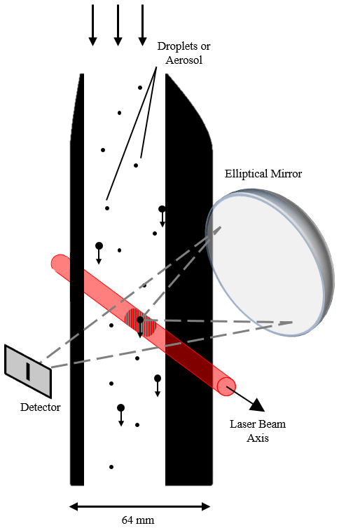
Figure 1An illustration of the UCASS working principle: scattered light at the first focal point of the elliptical mirror is reflected onto its second. The magnitude of this light is proportional to the size of the particle causing the scattering.
A concentration can be derived from UCASS data using one of two methods: particle time of flight (ToF) through the UCASS laser beam – the width of which is fixed and known, and the velocity of the UCASS itself – normally measured using a pitot tube. The former has the advantage of being the most direct measurement of sample area velocity, while the latter has the advantage of reliability and independence from particle size. The dependence of ToF on particle size originates from the method by which UCASS electronics calculates it – that is, the time between a pulse rising and falling above and below a threshold amplitude. Since the pulses can be assumed to be roughly Gaussian, two pulses with different maximum amplitudes through the same laser beam thickness would rise and fall above and below any threshold at different times. This difference is greater with threshold voltage height, and since the threshold must be above normal noise levels, the variation is significant with increased particle size. Figure 2 shows an illustration of this effect. The concentration derivation methods used are discussed further in Sects. 3 and 4.
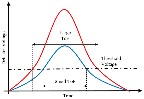
Figure 2An illustration of the ToF dependence on particle size for UCASS measurements. The red and blue lines represent large and small particles, respectively, for the same laser beam thickness.
The data from UCASS are available through its serial peripheral interface (SPI). Each data-point consists of the following for a given time interval: the particle counts in each of the 16 size bins; the mean particle ToF for bins numbered 1, 3, 5, and 7; the sampling period – the amount of time UCASS records particles for a datum; and some debugging information. The debugging information includes: the amount of particles with an extremely short or long ToF, which is used to filter out noise; the cumulative sum of all the particles counted, which is used to verify the data has been logged properly; and the amount of particles that have been rejected due to being outside of the sample volume, which is used to determine if co-incidence is likely.
The three main limitations of the UCASS–fixed-wing UAV combination are airspeed, angle of attack (AoA), and endurance. Airspeed is a limitation due to the bandwidth of the transimpedance amplifier (TIA), which converts the current from the photodiode into a scaled voltage. The cut-off frequency of the TIA is approximately 417 kHz, meaning that the maximum pulse width of the signal produced by a particle scattering light onto the photodiode is 2.4 µs. Since the thickness of the laser beam at the sample area is 60 µm, a maximum airspeed of 25 m s−1 was allowed in these experiments. Smith et al. (2019) showed that the particle number concentration measured by UCASS deviated from that measured by reference instrumentation when the airspeed increased above 15 m s−1. This was likely due to the drop off in amplification by the TIA as the frequency approached the cut-off. For this reason, the ideal airspeed for these experiments was treated as 15 m s−1; however, this was not always possible due to environmental and engineering factors, which are discussed in later sections.
The AoA – that is, the angle between the UCASS axis and inlet airflow vector – limit for the UCASS unit was defined in Smith et al. (2019) to be ±10∘. However, this assessment was only conducted for the UCASS alone, while not mounted on a platform. Therefore, this limit needed to be re-assessed for these experiments, the details of which are discussed in Sect. 3.
Water coating the light collection optics is an important factor to consider, not only with the UCASS instrument, but with all cloud probes. Both condensation and direct liquid deposition can attenuate the collected light, thus reducing the observed scattering cross-section magnitude. Since the temperature change between the sampling volume and ambient air was 0.04 K – see Sect. 3 for details – the condensation risk was negligible here, although it was considered that, at faster airspeeds, hydrophobic coatings may have been required on the collecting optics. Direct liquid deposition of water droplets onto the elliptical mirror – the largest exposed optical surface, and principal scattered light collector – was a greater concern. The UCASS elliptical mirror was designed with a surrounding circular groove in the chassis, in order to prevent the droplets – which get deposited on the inner airflow surfaces near the inlet – flowing onto the optical surfaces. The UCASS was tested with this inner chassis configuration in Smith et al. (2019), where it was found that droplet deposition on the optical surfaces was limited.
Since UCASS was originally designed as a single-use instrument (commonly utilised with balloon-based sounding systems, for example, Kezoudi et al., 2021a), the endurance must be questioned when operating a UCASS unit consistently throughout a research campaign. Specifically related to fixed-wing UAV operation, stresses from landings are likely to have the largest impact. Girdwood et al. (2020) introduces a ruggedised re-design of UCASS for multi-rotor UAVs. However, the stresses exerted on the instrument by a multi-rotor design are much higher than those exerted by a fixed-wing. Also, this design could not be directly translated onto a fixed-wing due to its size, since – unlike in the original UCASS – the laser and optics carrier protruded perpendicular to the chassis. For those reasons, the original design was chosen for fixed-wing use, but the endurance throughout the campaign was assessed and is presented in Sect. 4.
2.2 UAV and mounting
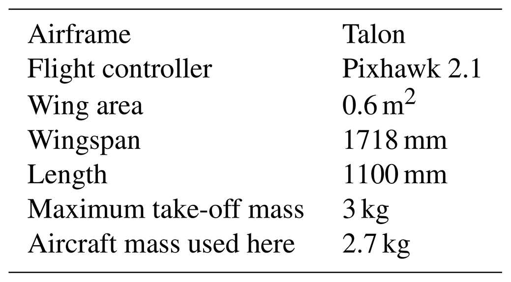
The UAV chosen for the evaluation of the nose-mounted configuration was the Talon UAV (X-UAV, Tian–Jie–Li Model Co., Ltd., China). The Talon platform was equipped for atmospheric measurements by the Finnish Meteorological Institute (FMI), with consultation from the University of Hertfordshire (UH) regarding the mounting of UCASS. This platform was chosen primarily for its flat top and wide fuselage, which provided an adequate mounting surface for the UCASS. An image of the UCASS mounted on the FMI-Talon is shown in Fig. 7b. The wide fuselage also provided enough space to mount the avionics, which included: a Pixhawk 1.2 flight controller (3DRobotics, 2013) with a global positioning system (GPS) and magnetometer; a Raspberry Pi Zero (RaspberryPi-Foundation, 2015) for the logging of UCASS data; a BME280 temperature, pressure, and humidity sensor; and a pitot-static tube to record the airspeed data essential for UCASS concentration measurements. The temperature and humidity measurements are not evaluated in this paper since they do not relate to the performance of UCASS, but are mentioned for the purpose of transparency, since they are often accompanying variables in datasets. The capabilities of the FMI-Talon are summarised in Table 1. The UCASS unit was mounted on the nose cone, with its inlet protruding well out of the fuselage boundary layer. This was influenced by the CFD-LPT experiments presented in Sect. 3.
In order to eliminate airframe-induced aerodynamic artefacts, the UCASS unit was positioned on mounts above the nose-cone. The UAV brushless electric motor was rear-facing and positioned at the back of the aircraft behind the tail, and, therefore, no aerodynamic artefacts resulting from the propeller wash were expected. In addition to this, the position of the motor means that no artefacts due to the charging – and subsequent deflection – of aerosols by its oscillating magnetic field are expected. The expected influence of the airframe aerodynamics on measurements, and the exact positioning of UCASS, are discussed in Sect. 3.
3.1 CFD-LPT method
The aim of these simulations – as with Girdwood et al. (2020) – was to define a series of UAV operating conditions, with particular focus on airspeed and AoA, in which UCASS would be able to make representative measurements, with reasonable tolerance.
The presented simulations were conducted using the Star-CCM+ commercial code. Two main mounting configurations were considered for the simulations: a configuration whereby the UCASS was positioned as far forward as the centre of gravity (CoG) tolerance of the FMI-Talon allowed, and a configuration were the UCASS was positioned further back from the end of the nose cone. Hereafter, these will be referred to as the fore and aft configurations, respectively. The former was expected to be advantageous only if the UCASS could be positioned far enough forwards to escape aerodynamic influence from the nose cone. The latter was expected to suffer from aerodynamic artefacts resulting from a non-zero AoA – that is, the angle between the axis of UCASS and the airflow velocity vector.
The domains for the fore and aft configurations are shown in Fig. 3a and b, respectively. The fore configuration shows the UCASS positioned as far forward as the CoG tolerance allowed. The domain was a two-dimensional slice through the FMI-Talon, bisecting the centre of UCASS and the UAV nose – indicated with the dashed purple circle and the black arrow in Fig. 3, respectively. The domain was a 2 m×2 m square, which was found by trial and improvement to suffer from no artefacts due to pressure wave reflections at the desired airspeed. The main point of interest for the simulations was the UCASS sample area, which was made the centre-point of both domains. In both domains, the air flowed in the direction of the blue arrow shown in Fig. 3a, and LPT droplets were injected from the right-hand wall. Since droplets are sampled when they cross a boundary, a boundary line was set up in the domain between regions (i) and (ii) – marked with the green line in Fig. 3 – which crossed the UCASS sampled volume. The pink lines around the perimeter of both domains represent “free-stream” regions, which are treated as infinitely extending regions with constant temperature and pressure – defined here as 280 K and 980 hPa, respectively.
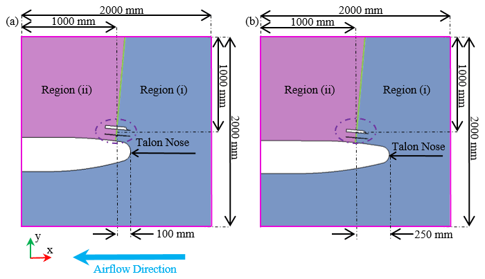
Figure 3Illustrations of the CFD-LPT domains for the two investigated configurations. Panel (a) shows the fore configuration and panel (b) the aft. The airflow direction and geometrical axes shown in panel (a) are consistent throughout. The UCASS is shown in the dashed purple circle, and the FMI-Talon nose cone is indicated. The purple lines represent free-stream boundaries, and the green line represents the divide between regions (i) and (ii) – which is where the LPT droplets are sampled.
The same mesh input parameters were used for both fore and aft configurations, since the differences in simulation convergence, simulation time, and accuracy were found to be to be small for the same mesh. A similar mesh dependency test to that presented in Girdwood et al. (2020) was conducted, but the full results are not shown here for the sake of brevity. The chosen base cell size of 10 mm, refined to 1 mm in the region surrounding UCASS and by the walls, was influenced by the mesh dependency test results. A polyhedral mesh was chosen since initial tests showed better convergence when compared to tetrahedral or hexahedral ones.
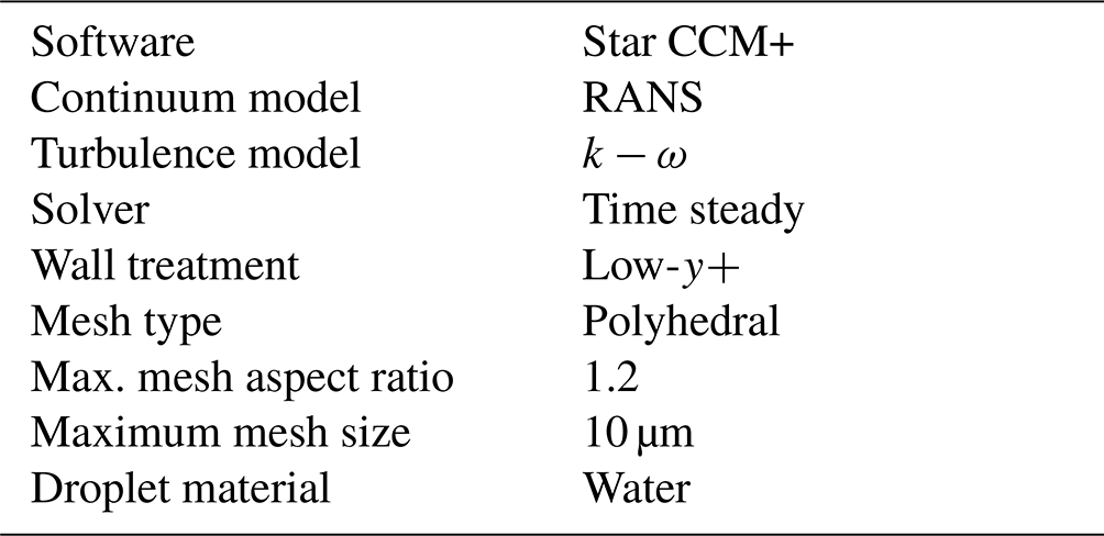
Since no motion needed to be simulated, the simulation was time-steady – meaning it was solved for one instance and iterated until converged. The simulation was considered to be converged when the continuity residual – that is, the difference in the average imbalance in continuity between adjacent solution iterations – was less than . Since direct numerical simulation was deemed to be too computationally expensive, a Reynolds-averaged Navier–Stokes (RANS) continuum model with a turbulence parameterisation model was used. The turbulence parameterisation model used was k−ω, which was chosen due to superior estimates of near-wall turbulence when compared to k−ϵ. The simulation and mesh parameters are summarised in Table 2.
3.2 CFD-LPT results and discussion
Since the aft configuration – shown in Fig. 3b – was only intended to be used if the UCASS could not be positioned out of the nose-cone influence due to CoG limits, the fore simulation was conducted first with an angle of attack of 0∘. Figure 4 shows a magnification of the pressure and velocity fields around UCASS and the FMI-Talon nose cone, in both fore and aft configurations – the left and right panels respectively. The colour of the background is the absolute pressure of the continuum, and the colour and direction of the glyphs show the velocity field. In the fore configuration, the airflow deflection off the nose cone of UCASS, as indicated by the yellow arrow in Fig. 4, was sufficiently large to create a leading edge vortex on the lower half of the UCASS inlet, which is indicated by the dashed black line. As shown in the background pressure plot of Fig. 4, this leading edge vortex compressed the airflow at the sample volume – indicated by the blue square – which caused the velocity to increase to 31 m s−1. As previously stated in Sect. 2.1, this velocity is well beyond what UCASS is able to tolerate due to the TIA bandwidth, and, therefore the fore configuration was abandoned at this stage. Droplets were not simulated for this geometry due to the inability of UCASS to measure them even if their trajectory and theoretical concentration would be unaffected by the leading edge vortex. The aft configuration, the results of which are shown in the right panel of Fig. 4, did not encounter this problem since a laminar boundary layer was attached to the aerodynamic surface of the FMI-Talon fuselage, meaning the airflow was directed parallel to the UCASS. This non-ideal positioning could have been subverted by the use of a custom built airframe – similar to Mamali et al. (2018) and Girdwood et al. (2020) – which would have more flexibility around positioning and could be designed around the UCASS. However, the design and construction of a custom airframe would be intensive and was beyond the scope of this research.
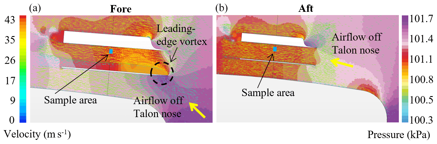
Figure 4A plot of the pressure and velocity fields of the fore and aft simulations, with an AoA of 0∘. The fore simulation results are shown in (a), and the aft results are shown in (b). The colour of the background is the absolute pressure of the continuum, and the colour and direction of the glyphs show the velocity field. The dashed black circle indicates a leading-edge vortex at the UCASS inlet in the fore simulation, the blue square indicates the UCASS sample volume, and the yellow arrow shows the airflow direction at the UCASS inlet.
The remaining simulations were conducted using the aft geometry in Fig. 3b. Since it was predicted that the aft configuration would be more sensitive to AoA changes, the first experiment was designed to keep droplet size and continuum velocity constant, while varying the free-stream velocity angle with respect to the FMI-Talon nose. The droplet diameter used was 20 µm, which was chosen to be slightly above a typical modal value of the droplet size distribution in a mature stratus cloud. Since the AoA limit for the UCASS without a platform is 10∘, the AoA range chosen was −20 to 20∘ – since an AoA of ±20∘ was deemed unlikely to be acceptable. Using Fig. 3 as a reference, a negative AoA was considered to be one that points downwards towards negative “y”. An AoA step of 5∘ was chosen as a balance of computation time and resolution. The injected concentration of droplets was 9 m−2, which was determined by experimentation to be the lowest concentration that could provide a statistically significant number of droplet streams at the UCASS sample volume. The value of 9 m−2 was largely abstract since the simulations were time steady and, therefore, conducted for one specific instance. The droplets were, therefore, simulated as parcel streams with inertia. The injected concentration of 9 m−2 corresponded to 10 parcel streams per 100 mm at the simulation inlet. The airspeed used for these simulations was 20 m s−1 since this was the target maximum airspeed for the UAV.
Since not enough droplets could be simulated to for a statistically significant quantity at the true 0.5 mm sample area of UCASS, a droplet was considered to have crossed the UCASS sample area if its trajectory crossed a plane coincident with the sample area, within 10 mm of its origin. As discussed previously in Sect. 2.1, there are two possible definitions of concentration from real UCASS data: ToF and pitot tube. Both definitions had to be assessed for differences, and, therefore, re-defined in the context of these CFD-LPT simulations. The droplet number concentration is defined here as
where Nc is the simulated number concentration (m−2), ns10 is the number of droplet parcel streams that intersect the sample plane within 10 mm of the sample area origin, A is the area around the sample area origin where a particle was considered to be sampled – 10 mm in this case – v is a velocity (m s−1), and t is the time (s) – which is an arbitrary scaling factor in this instance since time is steady. For all simulations, t was set equal to 1 for both the input and calculated output concentrations. The velocity, v, used depended on the sample volume calculation method. For the ToF equivalent, the droplet velocity at the sample plane was used; for the pitot tube, the freestream velocity of 20 m s−1 was used.
Figure 5 shows a plot of concentration and droplet airspeed through the sample volume versus AoA for the simulation. The red and blue lines are the concentration versus AoA calculated using the ToF and pitot tube methods, respectively, and the black dotted line is the mean velocity of the droplets as they cross the sample plane. The solid black line is the injected concentration of droplets at the inlet, and the shaded region is ±25 % of the inlet concentration, which was considered an acceptable error margin for concentration. This was because a light-weight OPC agreeing with a reference within this margin is generally considered robust, for example in Clarke et al. (2002). It was observed in the simulations that the concentration of droplets generally increased with AoA until 10∘, after which no droplet trajectories at all reached the sample area. This was because any AoA above this would cause boundary layer separation from the upper part of the fuselage, thus putting it under stall conditions and causing the majority of the droplets to be deflected around the resulting vortex.
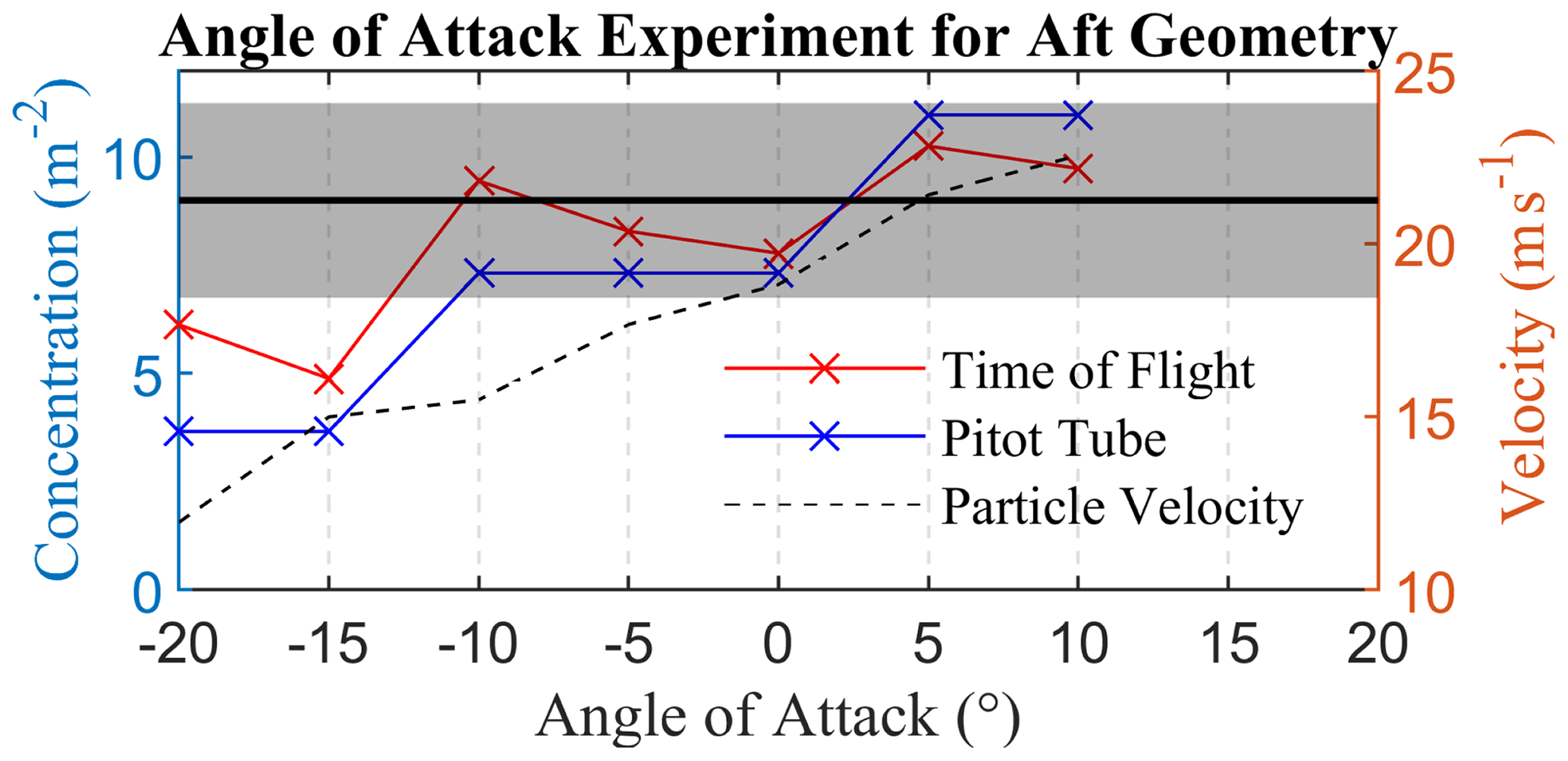
Figure 5Calculated droplet concentration against AoA for CFD-LPT simulated data. The solid black line shows the input concentration, and the black shaded region around it represents ±25 % of the input. The red and blue lines are the concentration data calculated using simulation equivalent droplet ToF and pitot tube airspeed, respectively. The black dotted line is the mean velocity of a droplet as its simulated trajectory crossed the UCASS sample area.
The general increase of droplet concentration with AoA is due to the convergence of continuum streamlines towards the upper part of UCASS before the boundary layer separates. This effect both increased the convergence of droplet parcel streams – and thus the pitot tube's estimated concentration – and the particle velocity at the sample plane. These effects conflict in their influence on the ToF particle concentration, since as velocity increases, the concentration calculated from Eq. (1) will decrease. This caused an increase in accuracy of the ToF concentration, which was within ±15 % of the injected concentration for AoAs between −10 and 10∘.
Both ToF and pitot tube-derived concentrations are found to be within acceptable limits, within the AoA range of −10 and 10∘. This is the same range as the UCASS without factoring in platform artefacts (Smith et al., 2019).
The effect of temperature and humidity fields on droplet size was considered, however – with an angle of attack of −10∘ – the temperature of the air at the sample volume is 280.19 K and the temperature of the air at the inlet was 280.23 K. At the time the paper was written, we did not consider the 0.04 K change in temperature to have a considerable effect on droplet diameter or the relative humidity of the air.
In addition to the AoA dependency, droplet size dependency was also tested in order to ensure that the shape of the size distribution was not affected. Since it was predicted that increased AoA would amplify size dependency, the simulations were run for AoAs of 0 and −10∘. The latter limit was chosen since, for negative AoAs, the inertia of larger droplets was predicted to force them away from the sample volume, which was closer to the upper edge of UCASS. The sizes used for the simulation were 3, 10, 20, and 40 µm, which were chosen since this range spanned the full size range of the UCASS in low-gain mode and was distributed approximately logarithmically. The results of this simulation are shown in Fig. 6, where the top panel shows the results for 0∘, and the bottom shows the results for −10∘. The graph legend is consistent with Fig. 5. The results of this simulation show that, for an AoA of 0∘, the size dependency is minimal – this can be seen in the top panel of Fig. 6. During these simulations – for an AoA of 0∘ – the particle velocity did not deviate much from 20 m s−1, meaning the ToF and pitot tube-derived concentrations were found to be similar, with a slight deviation for a size of 40 µm due to the slower acceleration within the UCASS inlet.

Figure 6Calculated droplet concentration against droplet diameter for two different AoAs. The solid black line shows the input concentration, and the black shaded region around it represents ±25 % of the input. The red and blue lines are the concentration data calculated using simulation equivalent droplet ToF and pitot tube airspeed, respectively. The black dotted line is the mean velocity of a droplet as its simulated trajectory crossed the UCASS sample area.
The size dependency results for an AoA of −10∘ are shown in the bottom panel of Fig. 6. This experiment revealed a larger concentration discrepancy for 40 µm droplets, which resulted from their larger inertia deflecting them away from the sample area. This discrepancy was beyond the ±25 % limit, which was considered acceptable. Beyond a re-design of the UCASS aerodynamics, however, there was little methodology that could rectify this. A large uncertainty of ±45 % – the percentage difference between the measured and input concentration of 40 µm droplets – is, therefore, placed on measurements of droplets above 30 µm, which is where the ToF-derived concentration strays beyond limits using linear interpolation.
The CFD-LPT simulations showed that ToF was, theoretically, the superior method for determining airspeed, since the concentration derived using this method was always closer to the input. However, in practice, this was not always the reality. This was because of the dependence of the ToF determined airspeed on a fixed beam width, which would change if the UCASS were to be subjected to large mechanical forces that could misalign the optics. In addition – as previously mentioned in Sect. 2.1 – ToF measured by the UCASS was dependent on the measured droplet size, so a calibration for each bin had to be applied. Also, if enough droplet measurements were not performed in a time-step integrated histogram, a statistically significant ToF measurement of that histogram cannot be performed. Pitot tube airspeed was, therefore, used when there were too few particles to perform a ToF measurement.
4.1 Field campaign method
The validation flights were undertaken during the Pallas Cloud Experiment (PaCE) in September 2020, at the Pallas atmosphere-ecosystem super site. The site, as shown in Fig. 7a, is located 170 km north of the Arctic Circle (67.973∘ N, 24.116∘ E), partly in the area of Pallas-Yllästunturi National Park (Lohila et al., 2015). Measurements were taken from 24 to 30 September; however stratus cloud was only present from the 28th to the 30th September. A fault in the data-logger used to gather flight data was persistent on the 30th, therefore only flights conducted on the 28th and 29th will be considered in this analysis. On each day, four profiles were conducted. Each profile consisted of an ascent and a descent through the entire cloud, which was approximately 1 km thick throughout the experiments. On 28 September, the mean wind speed throughout the day of flights was approximately 7 m s−1, the wind direction 200∘ from north, and the temperature 5 ∘C. On 29 September, the mean wind speed throughout the day of flights was approximately 5 m s−1, the wind direction 180∘ from north, and the temperature 8 ∘C. The wind direction is illustrated in Fig. 7d.
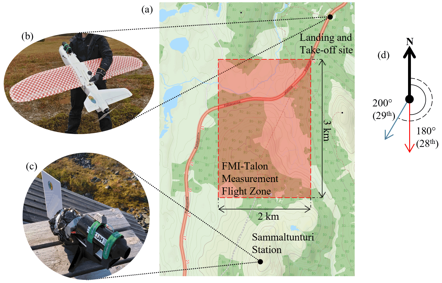
Figure 7A series of illustrations designed to give context to the measurement campaign. Figure 7a shows a map of the area including Sammaltunturi station – obtained from © OpenStreetMap contributors 2017. Distributed under the Open Data Commons Open Database License (ODbL) v1.0., the UAV landing site, and the flight operations zone in the red square; panel (b) shows the UCASS mounted to the FMI-Talon; panel (c) is an image of the UCASS – wind-vane system mounted to the station; and panel (d) shows the wind directions, measured by Sammaltunturi station, on 28 and 29 September with red and blue arrows, respectively.
The layered stratus cloud common to Pallas-Yllästunturi, combined with the airspace D527-Pallas reserved by FMI made this location perfect for the validation of UAV-based optical particle instruments. Since stratus cloud is normally laterally homogeneous within the distance scales discussed in this paper (the 2 km×3 km measurement area shown in Fig. 7a, Tsay and Jayaweera, 1984; Lawson et al., 2001), co-location errors between the UAV and station could be assumed to be minimal. The measured particles within the stratus cloud were all assumed to be water droplets, therefore the calibration look-up table for UCASS was made using a refractive index of 1.31+0i – the refractive index of water. Cloud droplets were considered the ideal validation particle since the UCASS calibration relies on Mie scattering, and the droplets can be assumed to be spherical. Water droplets also exhibit low absorption of 650 nm light – the wavelength of the UCASS laser. This is beneficial since absorption can cause artefacts in particle size measurements that utilise scattering like UCASS.
For comparative data, instruments were mounted on the roof of Sammaltunturi station, which was located on a hill 565 m above sea level (a.s.l.). The instrument chosen for the comparison was an identical UCASS unit, with the same TIA gain, oriented into the wind via the means of a wind vane and turret system, an image of which is shown in Fig. 7c. The only differences in the data between the two UCASS units would be due to platform artefacts, since they were otherwise identical. The aspiration airflow for UCASS was provided by the wind. The minimum airflow required for UCASS operation is 3 m s−1, since particles that produce longer ToFs than this are rejected in a firmware noise filter. At all instances during the campaign, the wind speed was faster than 3 m s−1. The wind speed for each UCASS data-point was measured using an anemometer on Sammaltunturi station. The UCASS – wind-vane set-up was secured to the roof each morning, before the daily flights started, and removed after flying was stopped for the day. This was to prevent damage to UCASS during the night, which may cause optical misalignment.
The FMI-Talon ascents and descents were conducted utilising a mixture of spiral patterns and wind-parallel patterns – both of which are commonly conducted in the literature (Martin et al., 2011; Mamali et al., 2018). The conducted flight patterns are summarised in Table 3, and the number concentration profiles are shown for context in Fig. 8. The purpose of this was to compare the two patterns to determine which is superior for UCASS measurements. Beyond the limits of the stratus cloud, when insufficient particles were present, the pitot tube airspeed was used to derive a sample volume. Within the cloud ToF was used. It was also observed that within the cloud, the pitot tube would become blocked, which caused the airspeed reported by the pitot tube to increase beyond physically possible limits. Not only did this render pitot tube measurements of sample volume impossible, the FMI-Talon also had to be manually piloted through the cloud since the large over-prediction in airspeed would cause the autopilot to stall the aircraft. Data from UCASS were recorded at 0.5 s intervals by a Raspberry Pi Zero (RaspberryPi-Foundation, 2015); pitot airspeed, attitude, and GPS data were recorded by the flight controller; and temperature, pressure, and humidity were recorded by a separate Raspberry Pi. The flights considered for analysis were the only flights for which all three data loggers were operating.
Table 3A table detailing the profile types of the UAV flights considered for analysis. The profile IDs are shown for the ascending and descending profiles, respectively.
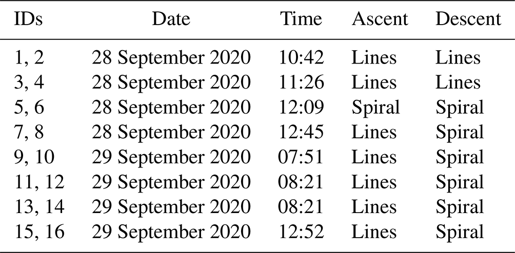
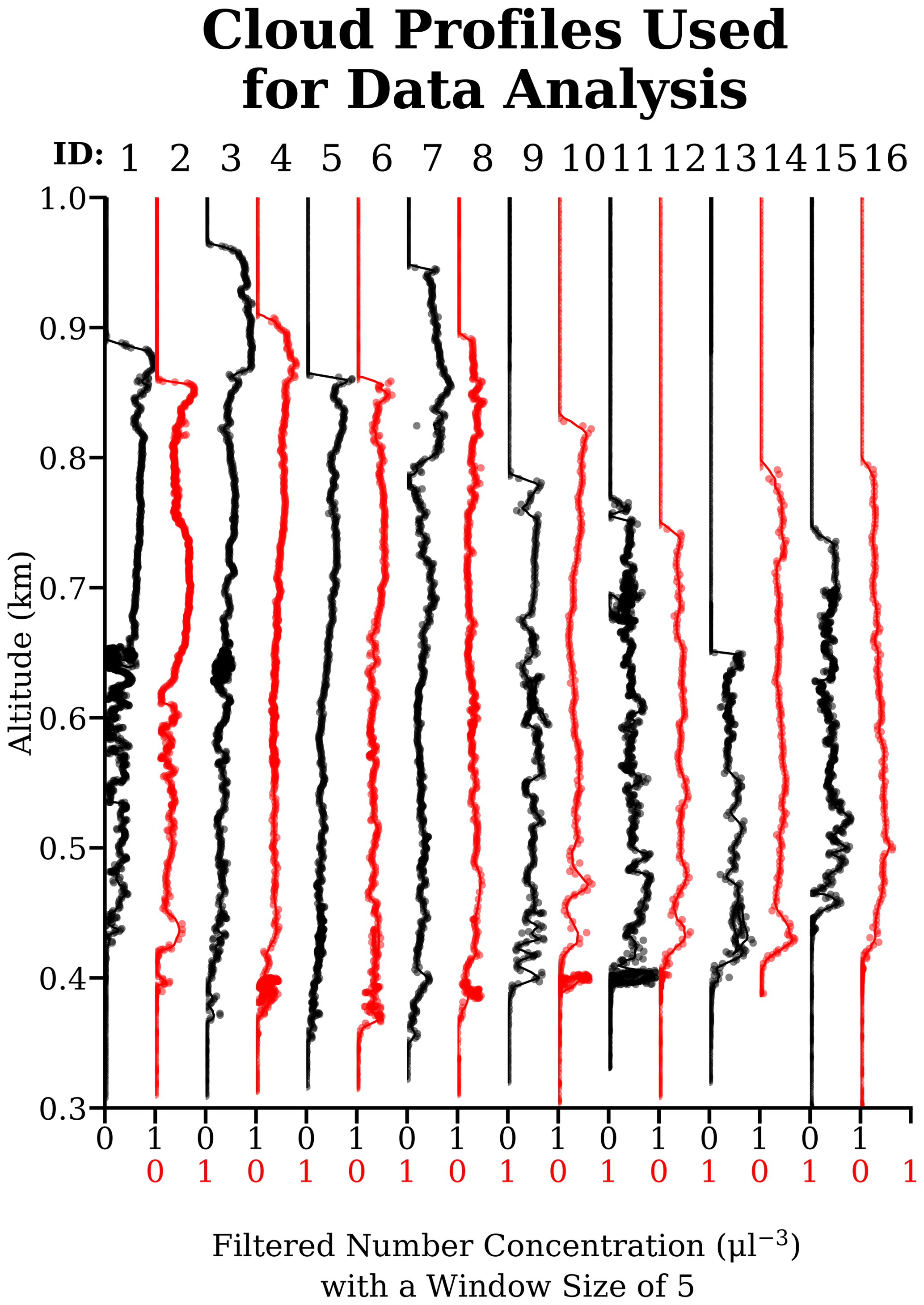
Figure 8The number concentration profiles through the stratus cloud, shown for the context of the campaign. The profile ID is shown above each panel and is consistent with Table 3. The ascending profiles are shown in black, and the descending profiles are shown in red.
The data were filtered based on two criteria, the first of which was a maximum airspeed limit, which was set to 20 m s−1. This was set because, even though the cut-off frequency of the TIA corresponds to an airspeed of 25 m s−1, the CFD-LPT simulations revealed that a droplet could travel faster through the UCASS sample area than the free-stream depending on AoA. An airspeed limit of 20 m s−1 ensures that, for all valid AoAs, the airspeed through the sample area never exceeds 25 m s−1. The second was an AoA limit defined as ±10∘, resulting from the CFD-LPT simulations in Sect. 3. AoA was defined here as the angle between the UAV axis and the resultant airspeed vector. The resultant airspeed vector is equal to the sum of the wind-speed vector, the vertical velocity of the UAV, and the UAV airspeed vector. The UAV airspeed vector was defined as
where Va is the UAV airspeed vector, Vpit is the pitot tube airspeed, ϕ is the UAV elevation angle, and θ is the azimuth angle of the UAV with respect to north – these were calculated from the pitch, roll, and yaw angles of the UAV. The angles and velocities are illustrated in Fig. 9 for clarity. Equation (2) is a normalised vector parallel to the UAV axis multiplied by the UAV airspeed (Vpit). Since wind-speed was considered likely to change as the UAV ascended, the wind angle measured by Sammaltunturi station was assumed constant with altitude, and the difference between the UAV ground speed and the “xz” component of the airspeed was used to calculate the wind-speed vector. This was given by
where
αw is the wind angle clockwise from north measured by Sammaltunturi station; Vw is the wind-speed vector; Vxz,a is the “xz” component of UAV airspeed; and Vxz,g is the UAV ground speed (Vg) expressed in vector form. The vertical velocity of the UAV was given by
where Vv is the vertical speed reported by the flight controller. The resultant airspeed vector was then given by
therefore, AoA was finally defined as
The Va used in Eq. (8) could be replaced with any vector parallel to UCASS, but this was used since it was already calculated in Eq. (2). The wind measurements produced via this method were not considered accurate nor reliable enough to be utilised in scientific datasets, simply because they were not validated here and were likely to suffer from measurement artefacts. However, they were considered robust enough to be used as rejection criteria for the UCASS particle spectrum data.
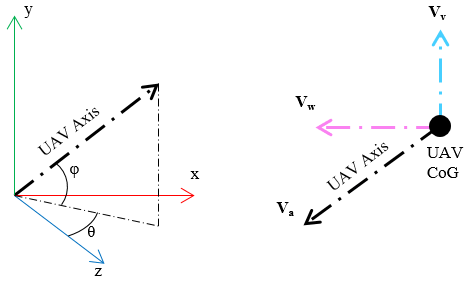
Figure 9An illustration clarifying the angle and velocity variable definitions used for the computation of AoA.
4.2 Field campaign results and discussion
Figures 10 and 11 show a comparison of against droplet diameter, measured by the FMI-Talon and Static UCASS when coincident, for 28 and 29 September, respectively. The blue and orange bars represent the measured in each bin of the FMI-Talon UCASS and the Static UCASS, respectively. The effective diameters recorded by both UCASS units are also shown on the plot. The effective diameter, as in Korolev et al. (1999), was defined as the ratio of the third and second statistical moments; that is, for binned UCASS data,
where Deff is the effective diameter, and ni is the number concentration in bin i, which has the geometric mean diameter Di. The take-off time and date of each flight are also shown in the bottom left corner. In each figure, the left-hand column of sub-figures shows data gathered on the ascending profile, and the right-hand column shows that gathered on the descending profile. The was calculated from
where cn,i is the number concentration in bin i, Dl,i is the lower size bin boundary of bin i, and is the lower size bin boundary of bin i+1. The FMI-Talon data used in Figs. 10 and 11 was averaged over a 40 m vertical distance – centred on the station altitude. The static UCASS data was averaged over 10 s – centred on the instance the Talon passed the altitude of Sammaltunturi station.
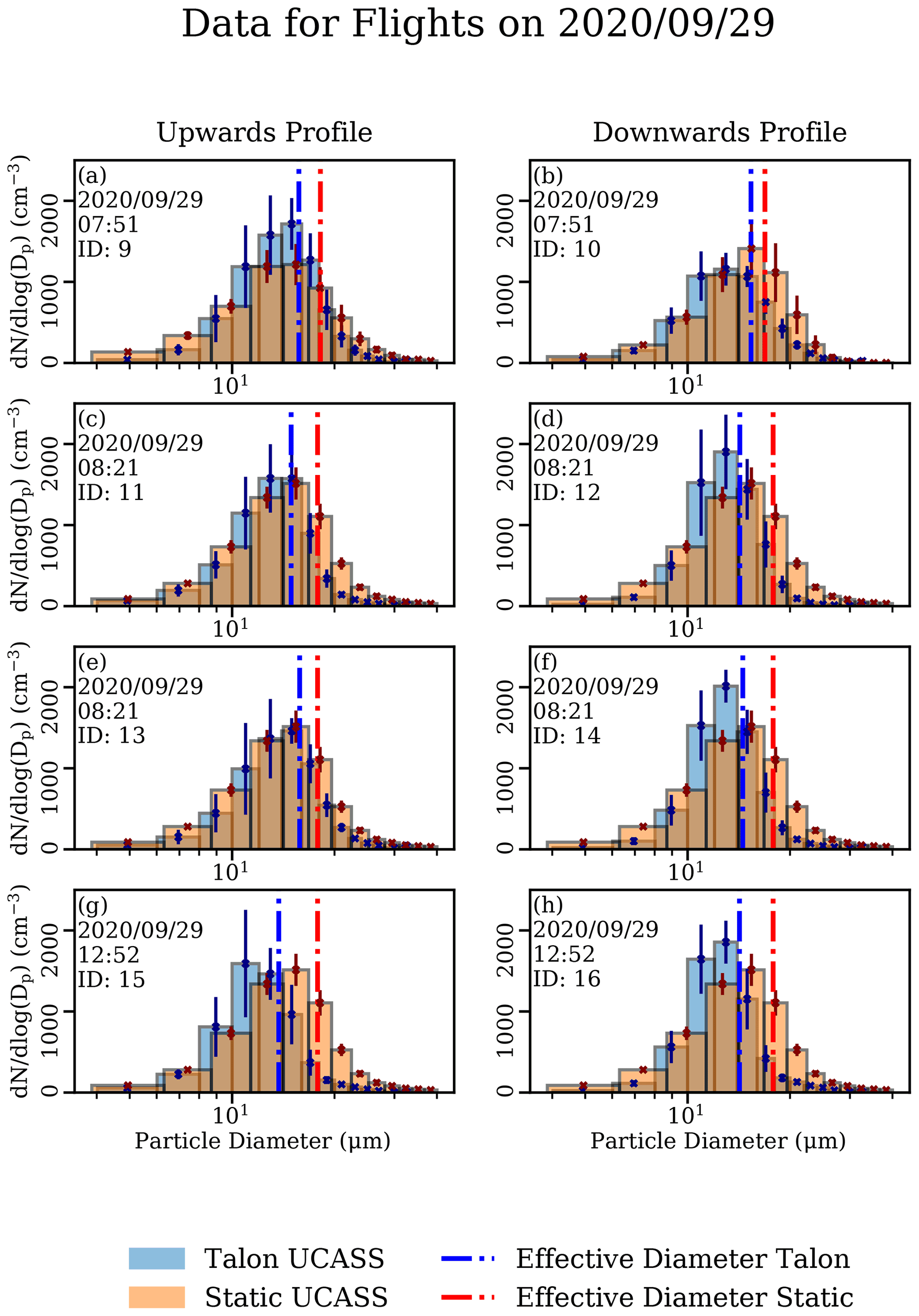
Figure 10Plots of plotted against droplet diameter for the flights conducted on 28 September 2020. The column of plots (a, c, e, g) is the data taken on the ascent, and the column of plots (b, d, f, h) is that taken on the descent. The thickness of each bar is a UCASS bin, the orange bars are the static UCASS data, and the blue bars are the FMI-Talon – UCASS data. The dashed red line is the effective diameter for the Static UCASS data, and the dashed blue line is that of the FMI-Talon – UCASS data. The profile ID stated is consistent with Table 3.
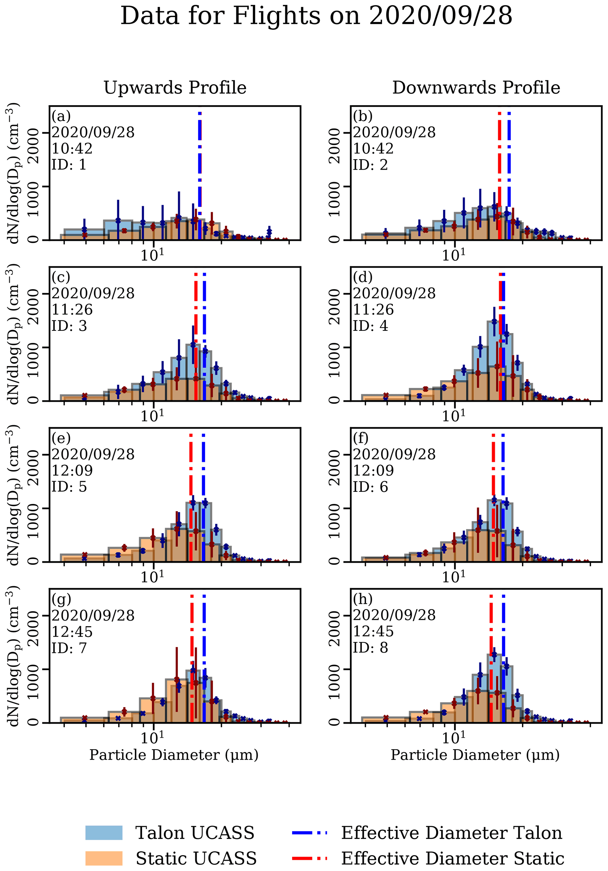
4.2.1 Measured diameter
The effective diameter measured by the UAV on 28 September overall was within 15 % of that measured by the static UCASS. However, there was an observed increase in the difference between the UAV and reference data with time, which would normally point to a calibration discrepancy caused by an offset in optical alignment. However, on the 28th, the effective diameter measured by the static UCASS was smaller. This was unusual because the FMI-Talon UCASS had undergone much larger stresses, which would cause it to measure lower than the static UCASS if a calibration offset in alignment was the case – since it is unlikely that an offset in alignment would increase the intensity of light incident to the photodiode. This trend can be seen in Fig. 12 in the points under the blue line. Laser mode hopping resulting from a temperature change was considered as a possible cause; however, the temperature only changed by 0.9 ∘C throughout the day of flights, which was not enough to cause a significant perturbation in laser wavelength, and, therefore, the measured effective diameter.
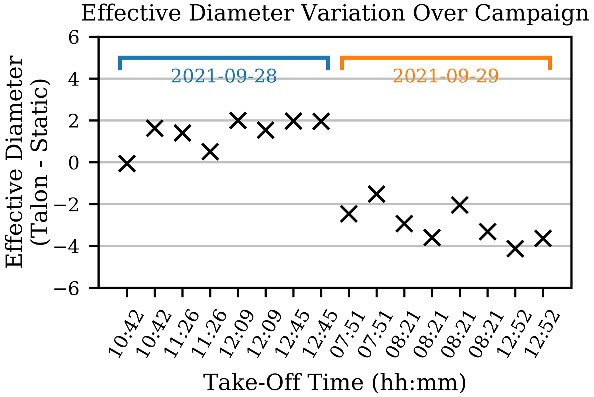
Figure 12A plot of the difference in effective diameter between the station mounted UCASS and the UAV mounted UCASS over the progression of the campaign. The 2 d discussed are highlighted in blue and orange.
Since the static UCASS was left immersed in the stratus cloud for an extended period of time, it was observed that some water droplets accumulated on the elliptical mirror – which was the largest exposed optical surface. These water droplets likely caused extinction of the scattered light from the droplets before it reached the photodiode. The decreased intensity of the photodiode incident light would cause under-sizing of the droplets, which would lead to a gradual decrease in effective diameter over time. Since this trend was observed in the data in Fig. 12, this was treated as the most probable cause for the increase of discrepancy in effective diameter over time. When the wind-vane – UCASS rig was re-attached on the station roof on the 29th, the UCASS was oriented in its mount with the mirror on top to reduce the number of droplets that were deposited on the mirror via gravitational settling. However, some droplets were still observed to be deposited on the mirror, which indicated that a proportion of the droplets settle via turbulent deposition or droplet shedding. This would require a re-design of the internal UCASS aerodynamics, similar to Korolev et al. (2013a).
On 28 and 29 September, a larger difference in effective diameter between the static UCASS and FMI-Talon UCASS was measured, which can be seen in Fig. 11. Contrary to measurements taken on the 28th, the static UCASS measured a larger effective diameter than the FMI-Talon UCASS, which can be more clearly seen in Fig. 12 under the orange line. The most likely cause for this was an offset in alignment in the FMI-Talon UCASS causing less light to be focused on the photodiode, and thus a smaller diameter to be measured. Since there was a significant step in the measured effective diameter between the 28th and the 29th, the most probable cause of the alignment offset was deemed to be transportation of the UCASS unit to or from the UAV launch site.
This alignment offset can be seen in Fig. 13, which is a plot of the UCASS instrument response – a 12-bit analogue to digital converter (ADC) value – against scattering cross section diameter, created from calibration data collected before and after the campaign with the same unit. A large differential can be seen between the two curves, particularly for droplets that would produce an ADC output of 1000 or higher. For example, a droplet that produces an ADC output of 3000 would be sized as 30 µm using the calibration data taken before the campaign, and 36 µm using that taken after the campaign. All the data discussed here used the calibration conducted prior to the campaign. The re-calibration data were not applied retroactively, since there would be a combination of steady shifts and discrete steps in calibration offset that would be difficult to account for and interpolate. In addition, flights that were not analysed here were also performed after 29 September, which would have caused calibration offsets that would not be applicable to these data. The degradation in UCASS alignment over the course of the campaign points to a need for a mechanical re-design of UCASS before its regular utilisation on fixed-wing UAVs, similar to that conducted in Girdwood et al. (2020). However, one single unknown event – as opposed to a gradual offset over time – between the 2 d appears to be the source of the misalignment, since there is a large step in the effective diameter differential between the 2 d considered.
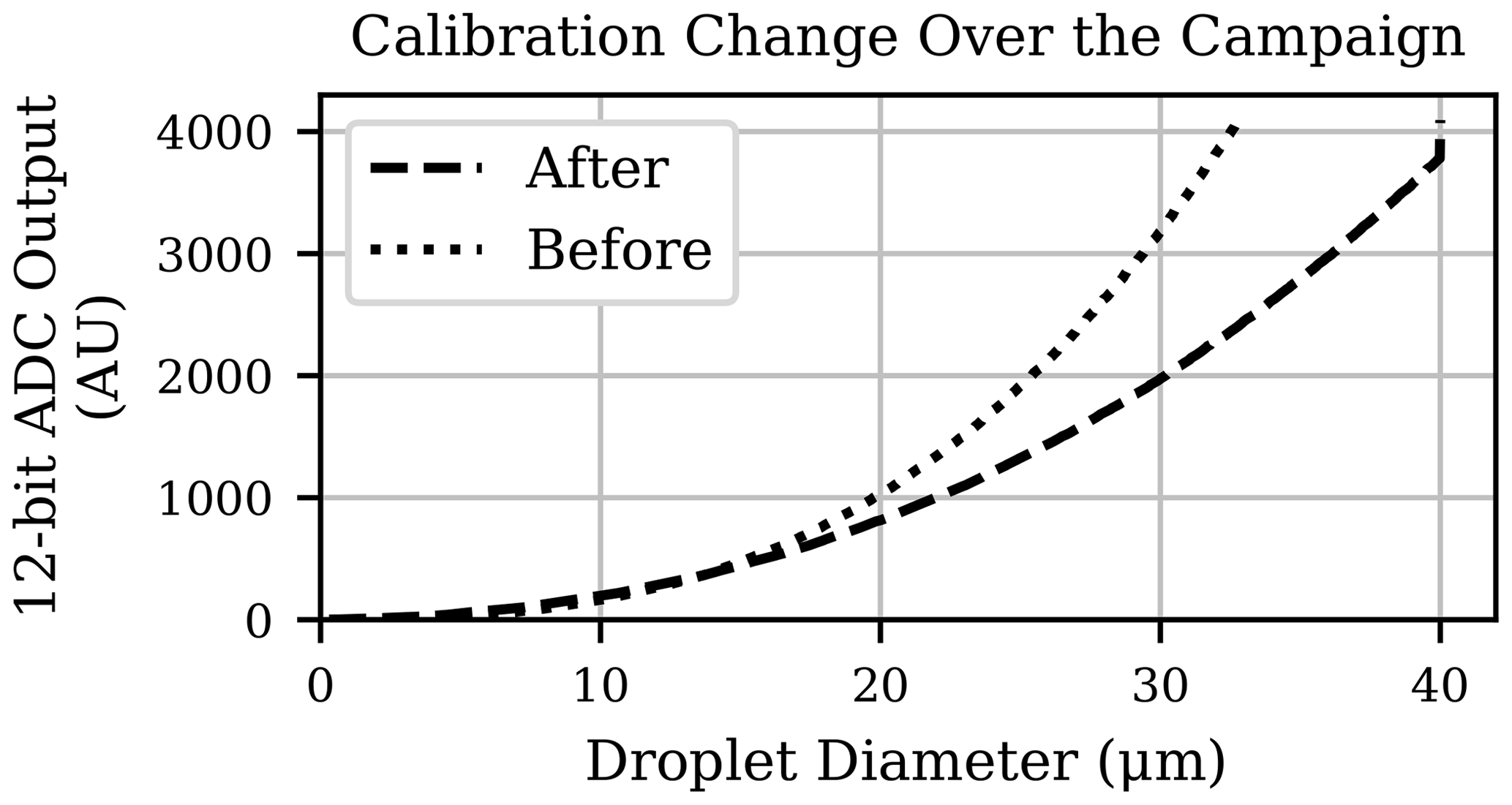
Figure 13A plot of the two instrument response curves – that is, 12-bit ADC output versus scattering cross section diameter – from calibration data collected before and after the campaign.
4.2.2 Measured concentration
The concentration measured by the FMI-Talon and Static UCASS units agreed within 15 % in all cases, apart from profiles 3, 4, 5, 6, and 8. The for these profiles can be seen in Fig. 10c through f, and h. In each case, the concentration measured by the FMI-Talon–UCASS was larger than that measured by the wind-vane–UCASS. This was unusual since most artefacts that the FMI-Talon–UCASS could suffer from – for example, large AoA values – would cause its measured concentration to decrease. Indeed, regression of the absolute number concentration differential and AoA yielded p values much larger than 0.05, indicating low statistical significance. Additionally, the difference in effective diameter for the measurements conducted on the 28th was minimal, and AoA effects would cause a shift in the measured size distribution towards smaller sizes, as demonstrated in Sect. 3. A difference between profile type – that is, spiral versus wind-parallel lines – was also considered as a possible cause; however the flights departing at 11:26 UTC utilised a wind-parallel profile, and the spiral descent profiles conducted on the 29th did not suffer from the same concentration differential.
While the regression of the absolute number concentration differential and airspeed yielded a large “p” value over the whole campaign, when only the data for the 28th of September were considered, the “p” value was 0.006 – which can be seen in Fig. 14. The more rigid correlation on the 28th than the 29th indicated a dependence of the airspeed induced concentration differential on another variable, which changed between the 2 d. Initial observations revealed that the variation in pitch, roll, and yaw of the aircraft were much higher on the 28th than on the 29th. For a quantitative definition, the root mean square (RMS) of the signal was used. In order to remove larger oscillations in the data, which occurred naturally as a response to wind speed changes, the signal was first normalised against a filtered version of itself, obtained using a moving average filter with a window size of 10 s. This window size was chosen because it was observed that these large variations did not occur on smaller timescales than this. This variable, γRMS, was defined mathematically as
where T1 and T2 are the time limits corresponding to when the UAV was at the altitude of Sammaltunturi station ±20 m; t is time; w is the window size in seconds, which in this instance was 20 s; f(t) is the pitch, roll, and yaw (PRY) of the UAV as a function of time; and H(t) is the Heaviside function of time. This was then calculated for PRY, which were then multiplied together to give the total PRY variation.
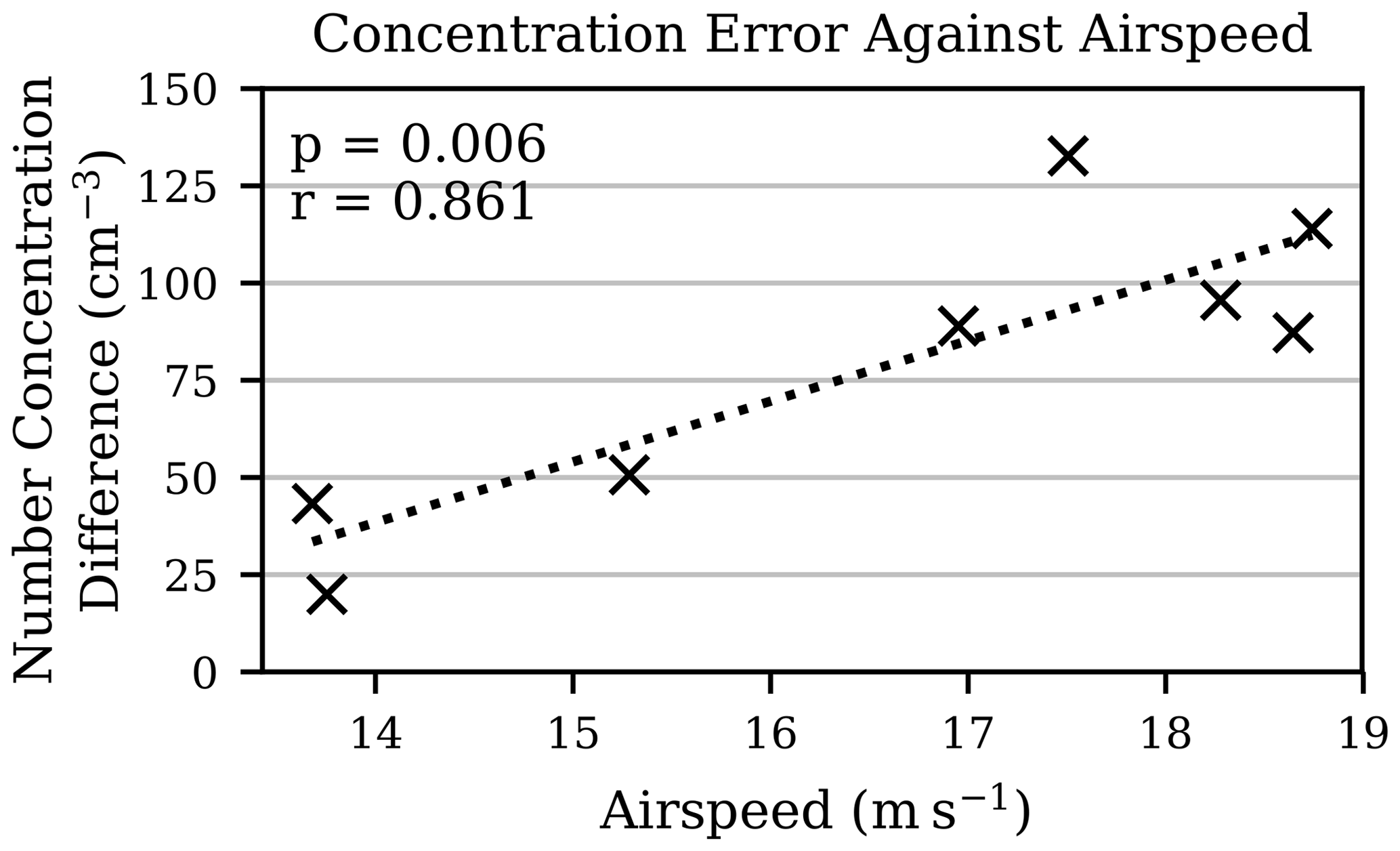
Figure 14A correlation plot of the absolute difference in measured number concentration between the FMI-Talon and Static UCASS units, and airspeed, for 28 September. The linear regression line and “p” value are shown.
Figure 15 shows the correlation of number concentration differential with PRY variation throughout the whole campaign. The regression yielded a “p” value of 0.018, which indicated statistical significance. The combination of the high Reynolds number resulting from a larger airspeed, and the large PRY perturbations encountered on the 28th, would result in an increased likelihood of turbulence. Turbulence can both cause a droplet to enter the sample area at an oblique angle and slow down the airspeed at the sample volume. Both of these effects would cause a larger ToF and, therefore, concentration to be recorded. Since the pitot tube was blocked throughout the cloud there was unfortunately no other airspeed measurement to compare with; however, turbulence was considered the most likely cause of the concentration differential. This result further exaggerated the need for smooth and steady sampling flight with a UAV. Since over half of the affected profiles were spiral-type, it was considered likely that the constant movement exacerbated the PRY variations. Since much of the data also had to be rejected from the spiral-type profiles, due to AoAs exceeding limitations defined in Sect. 3, the wind-parallel line profiles were considered more reliable for sampling with UCASS.
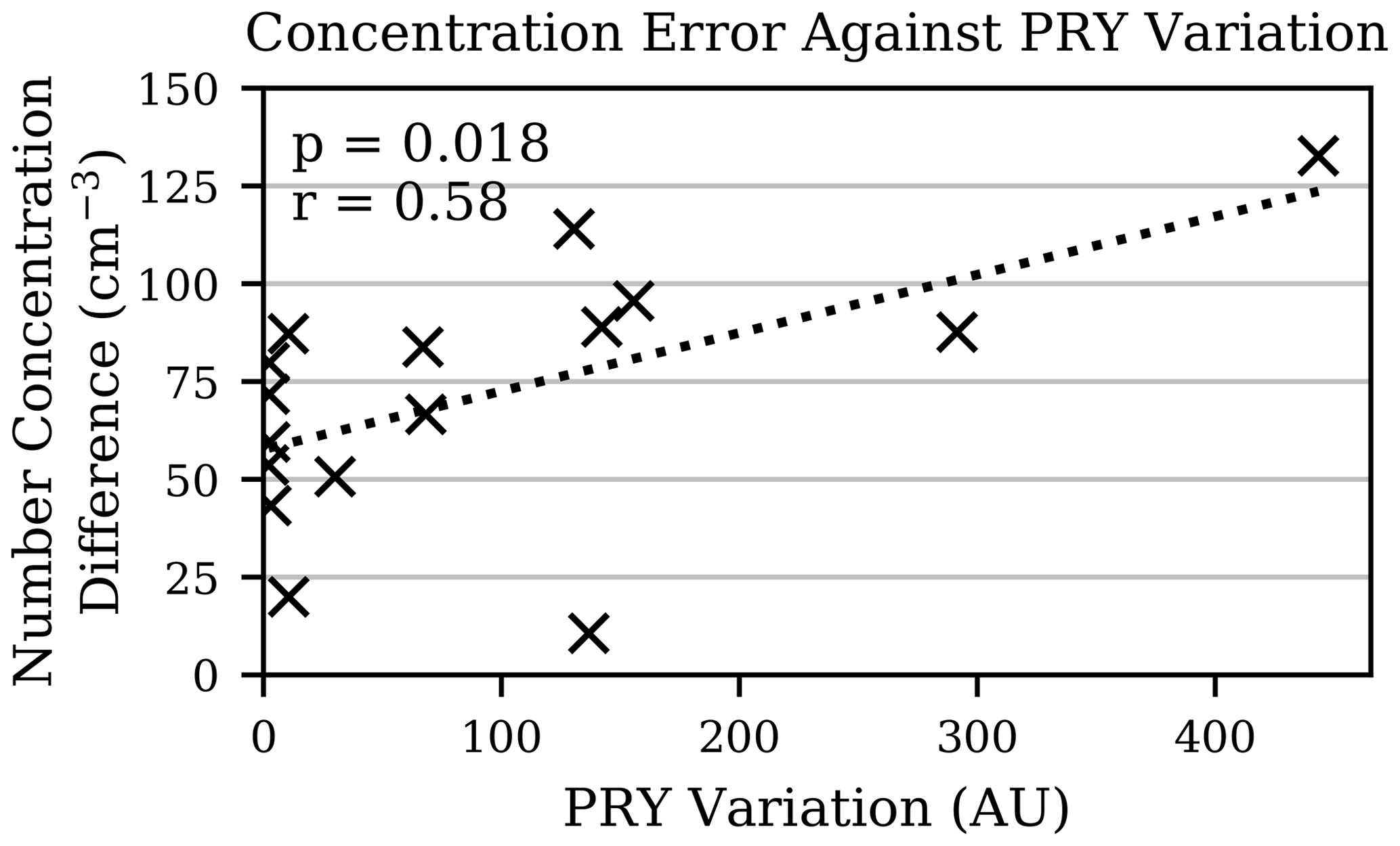
Figure 15A correlation plot of the absolute difference in measured number concentration between the FMI-Talon and Static UCASS units, and PRY variation, for the whole campaign. The linear regression line and “p” value are shown.
In this paper, a UCASS OPC was integrated on board a fixed-wing UAV – the FMI-Talon – and investigations were conducted into the accuracy and reliability of the combination. The UCASS, presented in Smith et al. (2019), utilised a gain configuration that allowed it to measure a size range of approximately 1 to 33 µm. Unlike in Girdwood et al. (2020), the UCASS was not re-designed for mechanical robustness. The FMI-Talon was capable of performing multiple sampling flights up to 1 km altitude, and functioning consistently throughout the day. It was also configured with temperature and humidity sensors that were not used in this research.
The investigations were composed of CFD-LPT simulations of the combinations and a field campaign examination involving an inter-comparison with reference instrumentation. The CFD-LPT simulations focused on two UCASS positions on the airframe. The first configuration involved the UCASS placed as far forward as the CoG tolerance of the FMI-Talon would allow. It was found that the UCASS could not be positioned forward enough to be beyond the influence of the deflection of the air by the nose cone, which caused a leading edge vortex to form on the UCASS inlet. Therefore, the second configuration had to be considered, that is, positioning the UCASS far enough back so that an attached airflow would be axial to the UCASS. This configuration was tested for a range of AoAs and simulated droplet sizes. It was found that the original AoA limit of UCASS, , was still acceptable with the FMI-Talon in this mounting configuration. However, a large uncertainty value of 45 % had to be placed on the concentration of droplets measured above 30 µm since their larger inertia caused a deflection around the UCASS sample area. The CFD-LPT simulations also compared two different methods for calculating droplet concentration: ToF and pitot tube. It was found that the ToF method provided a more accurate concentration but was unreliable when used in environments with a sparse ambient number concentration.
During the field campaign, the UAV was flown – utilising a mixture of spiral and wind-parallel profiles – through a stratus cloud up to approximately 1 km, and UCASS data were collected. A static UCASS mounted on a wind vane was positioned on the roof of a station 565 m a.s.l.; this provided the reference data to which the FMI-Talon–UCASS was compared. The analysed flights were conducted on 28 and 29 September 2020. Data were rejected according to AoA and airspeed criteria derived from the CFD-LPT simulations. For the measurements conducted on the 28th, the difference in effective diameter of the size distributions between the Talon and Static UCASS units was under 2 µm. However, the measurements conducted on the 29th revealed a high difference in effective diameter. The cause of this was found to be an offset in optical alignment – which likely occurred during transportation to and from the launch site, or a hard landing – which caused less light to reach the photodiode and, therefore, smaller sizes to be recorded. This was proven to be the case by re-calibrating the UCASS unit after the campaign and observing the offset. This result pointed to a need for a mechanical re-design of UCASS, similarly to Girdwood et al. (2020), before its consistent utilisation on UAVs can be realised. Since a similar assessment of the longevity of light-weight OPCs on UAVs has not been performed; the authors expect that this will also occur in many other instruments.
A discrepancy in number concentration between the static and UAV UCASS units was also observed on some of the profiles conducted on the 28th, where the FMI-Talon–UCASS measured higher values than the static UCASS. The number concentration discrepancy correlated well with the UAV airspeed only for the flights conducted on the 28th. The variation in pitch, roll, and yaw given by Eq. (11) was found to correlate well with number concentration discrepancy throughout the campaign, but only reached high values on the 28th. The concentration discrepancy was, therefore, determined to be caused by turbulence induced by the combination of these two variables, which would cause droplets to enter the sample area at oblique angles that would increase their measured ToF, and, therefore, concentration. This effect points to the need for steady sample flights, under auto-pilot if possible. Auto-pilot, however, was not possible for this campaign since the pitot tube used to measure airspeed would become blocked in the cloud.
The spiral and wind-parallel profiles were both found to be acceptable. However, more data had to be rejected from the spiral profiles than the wind-parallel profiles due to AoA constraints, and the wind-parallel profiles appeared to induce less pitch, roll, and yaw variations. Therefore, the wind-parallel profiles are recommended, where possible.
Future work relating to this project will be largely focused on a design overhaul of the UCASS instrument to deal with the mechanical stresses encountered during an intensive UAV field campaign. The updated UCASS will also include an extended size range and particle-by-particle data as opposed to bins. Future work will also be conducted into evaluating the new UCASS for aerosol measurements.
The data used in this paper from the PaCE 2020 campaign can be accessed from https://doi.org/10.18745/ds.25048 (Girdwood, 2021).
The original draft of the paper was prepared by JG and reviewed and edited by all co-authors. The project was conceptualised by JG, WS, and CS. Data curation was conducted by JG and DB. The formal analysis was conducted by JG. Project supervision was the responsibility of WS and CS. Methodology was developed by JG and DB. Validation was conducted by JG. Software was created by JG and WS.
The contact author has declared that neither they nor their co-authors have any competing interests.
Publisher’s note: Copernicus Publications remains neutral with regard to jurisdictional claims in published maps and institutional affiliations.
We thank the Finnish Meteorological Institute for providing accommodation and logistical support throughout the Pallas Cloud Experiment 2020 campaign.
This paper was edited by Wiebke Frey and reviewed by two anonymous referees.
3DRobotics: Pixhawk 1.2, https://pixhawk.org/ (last access: 2 December 2020), 2013. a
Beard, K. V. and Ochs, H. T.: Warm-Rain Initiation: An Overview of Microphysical Mechanisms, J. Appl. Meteorol., 32, 608–625, https://doi.org/10.1175/1520-0450(1993)032<0608:WRIAOO>2.0.CO;2, 1993. a
Blyth, A. M.: Entrainment in Cumulus Clouds, J. Appl. Meteorol., 32, 626–641, https://doi.org/10.1175/1520-0450(1993)032<0626:EICC>2.0.CO;2, 1993. a
Clarke, A. D., Ahlquist, N. C., Howell, S., and Moore, K.: A miniature optical particle counter for in situ aircraft aerosol research, J. Atmos. Ocean. Tech., 19, 1557–1566, https://doi.org/10.1175/1520-0426(2002)019<1557:AMOPCF>2.0.CO;2, 2002. a
Douglas, A. and L'Ecuyer, T.: Quantifying variations in shortwave aerosol–cloud–radiation interactions using local meteorology and cloud state constraints, Atmos. Chem. Phys., 19, 6251–6268, https://doi.org/10.5194/acp-19-6251-2019, 2019. a
Girdwood, J.: FMI-Talon – UCASS PaCE2020, University of Hertfordshire [data set], https://doi.org/10.18745/ds.25048, 2021. a
Girdwood, J., Smith, H., Stanley, W., Ulanowski, Z., Stopford, C., Chemel, C., Doulgeris, K.-M., Brus, D., Campbell, D., and Mackenzie, R.: Design and field campaign validation of a multi-rotor unmanned aerial vehicle and optical particle counter, Atmos. Meas. Tech., 13, 6613–6630, https://doi.org/10.5194/amt-13-6613-2020, 2020. a, b, c, d, e, f, g, h, i
Kezoudi, M., Tesche, M., Smith, H., Tsekeri, A., Baars, H., Dollner, M., Estellés, V., Bühl, J., Weinzierl, B., Ulanowski, Z., Müller, D., and Amiridis, V.: Measurement report: Balloon-borne in situ profiling of Saharan dust over Cyprus with the UCASS optical particle counter, Atmos. Chem. Phys., 21, 6781–6797, https://doi.org/10.5194/acp-21-6781-2021, 2021. a
Korolev, A., Emery, E., and Creelman, K.: Modification and tests of particle probe tips to mitigate effects of ice shattering, J. Atmos. Ocean. Tech., 30, 690–708, https://doi.org/10.1175/JTECH-D-12-00142.1, 2013a. a, b
Korolev, A. V., Isaac, G. A., Strapp, J. W., and Nevzorov, A. N.: In situ measurements of effective diameter and effective droplet number concentration, J. Geophys. Res., 104, 3993–4003, https://doi.org/10.1029/1998JD200071, 1999. a
Korolev, A. V., Emery, E. F., Strapp, J. W., Cober, S. G., and Isaac, G. A.: Quantification of the Effects of Shattering on Airborne Ice Particle Measurements, J. Atmos. Ocean. Tech., 30, 2527–2553, https://doi.org/10.1175/JTECH-D-13-00115.1, 2013b. a
Laird, N. F., Ochs, H. T., Rauber, R. M., and Miller, L. J.: Initial precipitation formation warm Florida cumulus, J. Atmos. Sci., 57, 3740–3751, https://doi.org/10.1175/1520-0469(2000)057<3740:IPFIWF>2.0.CO;2, 2000. a
Lawson, R. P., Baker, B. A., Schmitt, C. G., and Jensen, T. L.: An overview of microphysical properties of Arctic clouds observed in May and July 1998 during FIRE ACE, J. Geophys. Res., 106, 14989–15014, https://doi.org/10.1029/2000JD900789, 2001. a
Lohila, A., Penttilä, T., Jortikka, S., Aalto, T., Anttila, P., Asmi, E., Aurela, M., Hatakka, J., Hellén, H., Henttonen, H., Hänninen, P., Kilkki, J., Kyllönen, K., Laurila, T., Lepistö, A., Lihavainen, H., Makkonen, U., Paatero, J., Rask, M., Sutinen, R., Tuovinen, J. P., Vuorenmaa, J., and Viisanen, Y.: Preface to the special issue on integrated research of atmosphere, ecosystems and environment at Pallas, Boreal Environ. Res., 20, 431–454, 2015. a
Mamali, D., Marinou, E., Sciare, J., Pikridas, M., Kokkalis, P., Kottas, M., Binietoglou, I., Tsekeri, A., Keleshis, C., Engelmann, R., Baars, H., Ansmann, A., Amiridis, V., Russchenberg, H., and Biskos, G.: Vertical profiles of aerosol mass concentration derived by unmanned airborne in situ and remote sensing instruments during dust events, Atmos. Meas. Tech., 11, 2897–2910, https://doi.org/10.5194/amt-11-2897-2018, 2018. a, b
Martin, S., Bange, J., and Beyrich, F.: Meteorological profiling of the lower troposphere using the research UAV “M2AV Carolo”, Atmos. Meas. Tech., 4, 705–716, https://doi.org/10.5194/amt-4-705-2011, 2011. a
RaspberryPi-Foundation: Raspberry Pi Zero, https://www.raspberrypi.org/products/raspberry-pi-zero/ (last access: 2 December 2020), 2015. a, b
Small, J. D. and Chuang, P. Y.: New observations of precipitation initiation in warm cumulus clouds, J. Atmos. Sci., 65, 2972–2982, https://doi.org/10.1175/2008JAS2600.1, 2008. a
Smith, H. R., Ulanowski, Z., Kaye, P. H., Hirst, E., Stanley, W., Kaye, R., Wieser, A., Stopford, C., Kezoudi, M., Girdwood, J., Greenaway, R., and Mackenzie, R.: The Universal Cloud and Aerosol Sounding System (UCASS): a low-cost miniature optical particle counter for use in dropsonde or balloon-borne sounding systems, Atmos. Meas. Tech., 12, 6579–6599, https://doi.org/10.5194/amt-12-6579-2019, 2019. a, b, c, d, e, f, g
Spanu, A., Dollner, M., Gasteiger, J., Bui, T. P., and Weinzierl, B.: Flow-induced errors in airborne in situ measurements of aerosols and clouds, Atmos. Meas. Tech., 13, 1963–1987, https://doi.org/10.5194/amt-13-1963-2020, 2020. a
Stocker, T. F., Qin, D., Plattner, G.-K., Alexander, L. V., Allen, S. K., Bindoff, N. L., Bréon, F.-M., Church, J. A., Cubasch, U., Emori, S., Forster, P., Friedlingstein, P., Gillett, N., Gregory, J. M., Hartmann, D. L., Jansen, E., Kirtman, B., Knutti, R., Krishna Kumar, K., Lemke, P., Marotzke, J., Masson-Delmotte, V., Meehl, G. A., Mokhov, I. I., Piao, S., Ramaswamy, V., Randall, D., Rhein, M., Rojas, M., Sabine, C., Shindell, D., Talley, L. D., Vaughan, D. G., and Xie, S.-P.: Technical Summary, in: Climate Change 2013: The Physical Science Basis. Contribution of Working Group I to the Fifth Assessment Report of the Intergovernmental Panel on Climate Change, edited by: Stocker, T. F., Qin, D., Plattner, G.-K., Tignor, M., Allen, S. K., Boschung, J., Nauels, A., Xia, Y., Bex, V., and Midgley, P. M., Cambridge University Press, Cambridge, United Kingdom and New York, NY, USA, https://doi.org/10.1017/CBO9781107415324, 2013. a
Tsay, S.-C. and Jayaweera, K.: Physical Characteristics of Arctic Stratus Clouds, J. Appl. Meteorol. Clim., 23, 584–596, https://doi.org/10.1175/1520-0450(1984)023<0584:PCOASC>2.0.CO;2, 1984. a
Zelinka, M. D., Andrews, T., Forster, P. M., and Taylor, K. E.: Quantifying components of aerosol-cloud-radiation interactions in climate models, J. Geophys. Res.-Atmos., 119, 7599–7615, https://doi.org/10.1002/2014JD021710, 2014. a, b, c
Zeng, X.: Modeling the Effect of Radiation on Warm Rain Initiation, J. Geophys. Res.-Atmos., 123, 6896–6906, https://doi.org/10.1029/2018JD028354, 2018. a