the Creative Commons Attribution 4.0 License.
the Creative Commons Attribution 4.0 License.
 | 14 Apr 2022
The eVe reference polarisation lidar system for the calibration and validation of the Aeolus L2A product
Nikolaos Siomos
Alexandra Tsekeri
Alexandros Louridas
George Georgoussis
Volker Freudenthaler
Ioannis Binietoglou
George Tsaknakis
Alexandros Tavernarakis
Christos Evangelatos
Jonas von Bismarck
Thomas Kanitz
Charikleia Meleti
Eleni Marinou
Vassilis Amiridis
The eVe dual-laser/dual-telescope lidar system is introduced here, focusing on the optical and mechanical parts of the system's emission and receiver units. The compact design of the linear–circular emission unit along with the linear–circular analyser in the receiver unit allows eVe to simultaneously reproduce the operation of the ALADIN lidar on board Aeolus as well as to operate it as a traditional ground-based polarisation lidar system with linear emission. As such, the eVe lidar aims to provide (a) ground reference measurements for the validation of the Aeolus L2A aerosol products and (b) the conditions for which linear polarisation lidar systems can be considered for Aeolus L2A validation, by identifying any possible biases arising from the different polarisation state in the emission between ALADIN and these systems, and the detection of only the co-polar component of the returned signal from ALADIN for the L2A products' retrieval. In addition, a brief description is given concerning the polarisation calibration techniques that are applied in the system, as well as the developed software for the analysis of the collected signals and the retrieval of the optical products. More specifically, the system's dual configuration enables the retrieval of the optical properties of particle backscatter and extinction coefficients originating from the two different polarisation states of the emission and the linear and circular depolarisation ratios, as well as the direct calculation of the Aeolus-like backscatter coefficient, i.e. the backscatter coefficient that Aeolus would measure from the ground. Two cases, one with slightly depolarising particles and one with moderately depolarising particles, were selected from the first conducted measurements of eVe in Athens in September 2020, in order to demonstrate the system's capabilities. In the slightly depolarising scene, the Aeolus-like backscatter coefficient agrees well with the actual backscatter coefficient, which is also true when non-depolarising particles are present. The agreement however fades out for strongly depolarising scenes, where an underestimation of ∼18 % of the Aeolus like backscatter coefficient is observed when moderately depolarising particles are probed.
- Article
(10927 KB) - Full-text XML
- BibTeX
- EndNote


The calibration and validation (Cal/Val) of spaceborne instruments for Earth observation (EO) have traditionally relied on ground-based measurements provided by well-characterised reference systems (Holben et al., 1998; Pappalardo et al., 2014). The Aeolus mission (Reitebuch, 2012; Stoffelen et al., 2005), an atmospheric Earth Explorer Core mission of the European Space Agency (ESA), is not an exception, particularly with respect to the Cal/Val of the wind, aerosol, and cloud product from the Atmospheric Laser Doppler Instrument (ALADIN). Aeolus is designed to provide global profiles of the horizontal line-of-sight (HLOS) wind component in the troposphere and the lower stratosphere (Dabas, 2010; Stoffelen et al., 2006; Tan et al., 2008) through ALADIN, a sophisticated Doppler wind lidar (DWL; Paffrath et al., 2009; Reitebuch et al., 2009) and the only instrument on board the platform. ALADIN is a high spectral resolution lidar (HSRL) operating in the ultraviolet region of the spectrum at 355 nm wavelength, implemented in a transceiver configuration and tilted 35∘ from nadir (Lolli et al., 2013). The instrument utilises a circularly polarised emission and a multiple-interferometer receiver for the detection of the backscattered light from molecules and particulates (i.e. aerosols and clouds) to the Rayleigh and Mie channels, respectively (Flamant et al., 2007). The Rayleigh and Mie signals are distinguished by considering the broader and the narrower scattered spectra for molecules and particulates, respectively, attributed to the Doppler effect (Imaki et al., 2005; Shipley et al., 1983). Besides the wind profiles, ALADIN is also capable of deriving particle optical properties such as the particle backscatter coefficient, the particle extinction coefficient, and the inverted lidar ratio, i.e. the backscatter-to-extinction ratio (BER) (Ansmann et al., 2007; Flamant et al., 2008). However, ALADIN's configuration enables the detection of only the co-polar component of the backscattered circularly polarised emission, resulting in the retrieval of the co-polar backscatter coefficient (see Appendix A). The missing cross-polar component is not negligible in the case of depolarising particles in the atmosphere, such as ice crystals (e.g. Mishchenko and Sassen, 1998), dust (e.g. Freudenthaler et al., 2009), pollen (e.g. Sassen, 2008), and volcanic ash (e.g. Ansmann et al., 2010) or stratospheric smoke (e.g. Gialitaki et al., 2020). For non-depolarising particles, the co-polar backscatter coefficient can be calculated from the theory considering the depolarisation of the molecules (see Appendix A) and can approximate the total backscatter coefficient well, an extensive aerosol optical property that is commonly measured from the lidar systems (Ansmann et al., 1992; Fernald, 1984; Klett, 1981; Sasano and Nakane, 1984). This is not the case, in the presence of depolarising particles, where the co-polar backscatter coefficient is significantly smaller with respect to the total backscatter coefficient. In such cases, related discrepancies of up to 75 % for ice crystals and up to 50 % for dust or ash particles can be expected for the co-polar backscatter coefficient with respect to the total backscatter coefficient (Flamant et al., 2007), and the Aeolus L2A products of the particle backscatter coefficient and the BER will be underestimated. The Cal/Val of the Aeolus L2A products is, thus, far more suitable with lidar systems with polarisation capabilities to identify ALADIN's inherent uncertainty for depolarising scenes. Such lidar systems have become increasingly popular within the aerosol remote sensing community (for instance, the European Aerosol Research Lidar Network, EARLINET, currently comprises 18 stations that perform linear polarisation measurements with lidars; Pappalardo et al., 2004).
In principle, the emitted linearly polarised light is backscattered, mainly with the same linear polarisation and partly depolarised, upon interaction with atmospheric targets which are non-spherical and randomly oriented (Mishchenko and Hovenier, 1995). The polarisation-sensitive detection of the collected backscattered signal is usually performed by separating the signal into two optical paths; the first (parallel or co-polar) contains the backscattered light with the original polarisation and half of the depolarised light, and the second (cross or cross-polar) contains the other half of the depolarised light (Gimmestad, 2008). There are also systems that rely on the detection of the total and cross-backscattered signals instead (Engelmann et al., 2016). In both cases, profiles of the aerosol volume linear depolarisation ratio can be calculated from the two signals.
For atmospheric layers containing randomly oriented particles and where multiple scattering is negligible, the lidar measurements of the linear depolarisation ratio are sufficient for validating the Aeolus circular polarisation products, since the relationship between the linear and circular depolarisation ratios is known from theory (Mishchenko and Hovenier, 1995; Roy and Roy, 2008). Hence, the linear polarisation products can be easily converted to circular polarisation products (see Appendix A), facilitating the validation of Aeolus L2A products in an indirect way. On the other hand, for depolarising scenes where the aforementioned assumptions are not valid due to particle orientation (e.g. of desert dust; Daskalopoulou et al., 2021; Mallios et al., 2021; Ulanowski et al., 2007; and cirrus clouds, for example, Myagkov et al., 2016; Noel and Sassen, 2005; Thomas et al., 1990) and/or multiple scattering effects inside the clouds (Donovan et al., 2015; Jimenez et al., 2020a; Schmidt et al., 2013), and even within optically thick aerosol layers (Wandinger et al., 2010), the linear to circular polarisation products conversion is not applicable, and a direct validation of the Aeolus L2A products is needed, using a polarisation lidar system with circularly polarised emission similar to ALADIN.
In this paper we present the eVe lidar system (Enhancement and Validation of ESA products), a combined linear–circular polarisation system designed to provide the Aeolus mission with ground-based reference measurements, facilitating the Aeolus L2A product validation, assessment, and optimisation. The system's design incorporates the necessary hardware elements to reproduce both the operation of ALADIN, that relies on circularly polarised emission, and the operation of a traditional polarisation lidar system with linearly polarised emission. Besides its main goal (i.e. to validate Aeolus L2A), the dual linear–circular configuration enables the examination of the conversion factors from linear to circular polarisation products for a wide variety of aerosol and cloud types. This procedure will consequently provide an evaluation of possible biases in Cal/Val studies performed with linear polarisation lidar systems (which are available worldwide). In addition, the eVe lidar can be used as the ground reference system for the validation of future ESA missions like EarthCARE (Illingworth et al., 2015).
Section 2 provides a brief description of the system, focusing on the mechanical and optical parts. Section 3 presents the polarisation calibration techniques that have been developed for eVe. The lidar signal processing and the optical products' retrieval algorithm are described in Sect. 4. Section 5 presents the first optical products of eVe for two selected cases measured over Athens. Finally, we summarise and conclude in Sect. 6. The conversion formulas from the linear to circular polarisation products, and vice versa, are given in Appendix A. Results from the quality assurance (QA) tests performed on the lidar are presented in Appendix B.
The eVe lidar has been constructed by Raymetrics S.A., Athens, Greece, in collaboration with the National Observatory of Athens and the Ludwig-Maximilians-Universität, Munich, Germany. The system has been designed to be a flexible and mobile ground-based lidar system, capable of operating under a wide range of ambient conditions. The system utilises two lasers, one emitting linearly and the other circularly polarised light, respectively, and two telescopes, each collecting sequentially the backscattered light from both lasers. The collected backscattered signals are recorded by five photomultiplier tubes (PMTs) in combined analogue and photon-counting mode (Licel GmbH, 2020). The three main components of the system are the lidar head, the positioner, and the electronics enclosure, as shown in Fig. 1. The lidar head is mounted on the positioner, and both of them are mounted on the electronics enclosure. The electronics enclosure and the lidar head are connected with two umbilical tubes that contain the lasers' cooling lines as well as the power and communication cables. Moreover, the electronics enclosure and the lidar head have independent cooling and heating systems, allowing the system to operate in ambient temperatures from 5 ∘C up to 45 ∘C. The system is also rain- and dust-proof, with an IP (Ingress Protection) rating of 55.
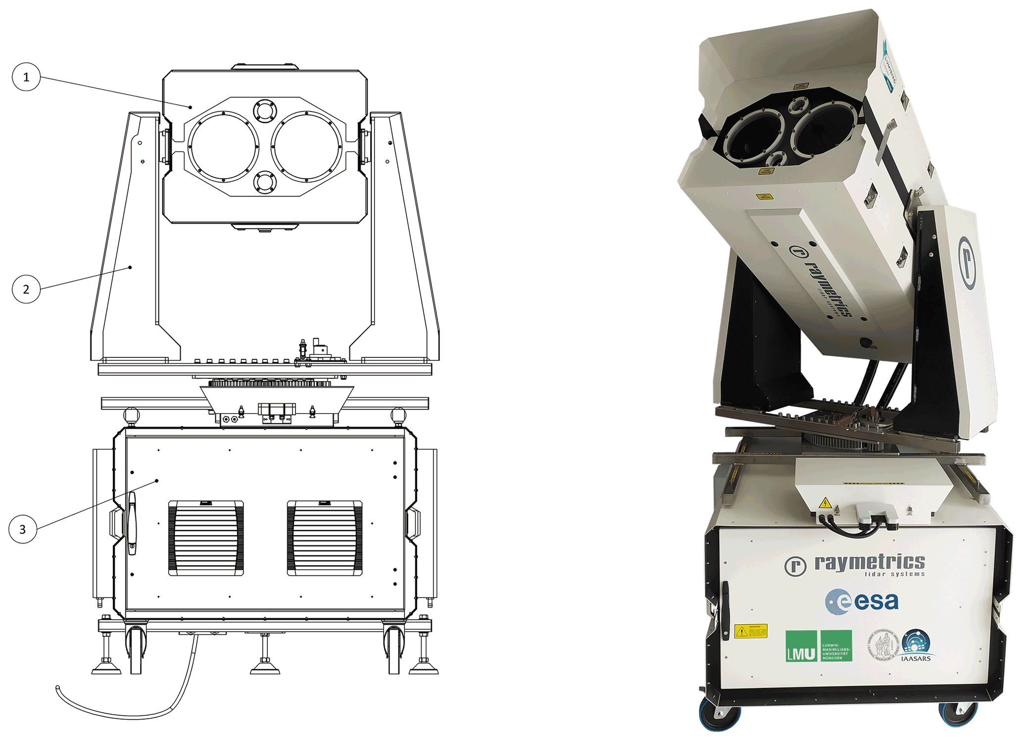
Figure 1The lidar head (1), the alt-azimuth positioner (2), and the electronic enclosure (3) of the eVe lidar system.
2.1 The lidar head
The lidar head consists of the emission unit and the receiver unit, for which a detailed schematic of the head's internal parts is presented in Fig. 2. The internal components of the lidar head are protected from the ambient atmospheric conditions by the head metal covers, two laser windows, and two telescope windows. The head covers can be easily and fully removed, providing a full access to the internal parts for maintenance and troubleshooting purposes. Three thermoelectric coolers are also installed to stabilise the internal temperature of the lidar head at 30±2.5 ∘C.
2.1.1 Emission
The emission unit contains two CFR400 model Nd:Yag lasers (LA and LB) manufactured by Lumibird S.A., both originally emitting linearly polarised laser pulses at 355 and 532 nm and elliptically polarised pulses at 1064 nm due to the housed harmonic generation module inside the lasers. According to the laser manufacturer, the laser pulses are emitted with a repetition rate of 20 Hz and energies of ∼89 and ∼100 mJ at 355 nm, 88 and ∼97 mJ at 532 nm, and ∼117 and ∼135 mJ at 1064 nm for LA and LB, respectively, before the emission optics. LB is equipped with one motorised rotated quarter wave plate (QWP) placed at 45∘ with respect to the original laser polarisation orientation, for converting the linear polarisation to circular only for the laser pulses at 355 nm. Hereafter, the QWP that is placed after LB in the emission unit will be called QWPE. Thus, LA emits linearly polarised pulses at 355 and 532 nm and elliptically polarised pulses at 1064 nm, while the LB emits circularly polarised pulses at 355 nm and elliptically polarised pulses at 532 and 1064 nm.
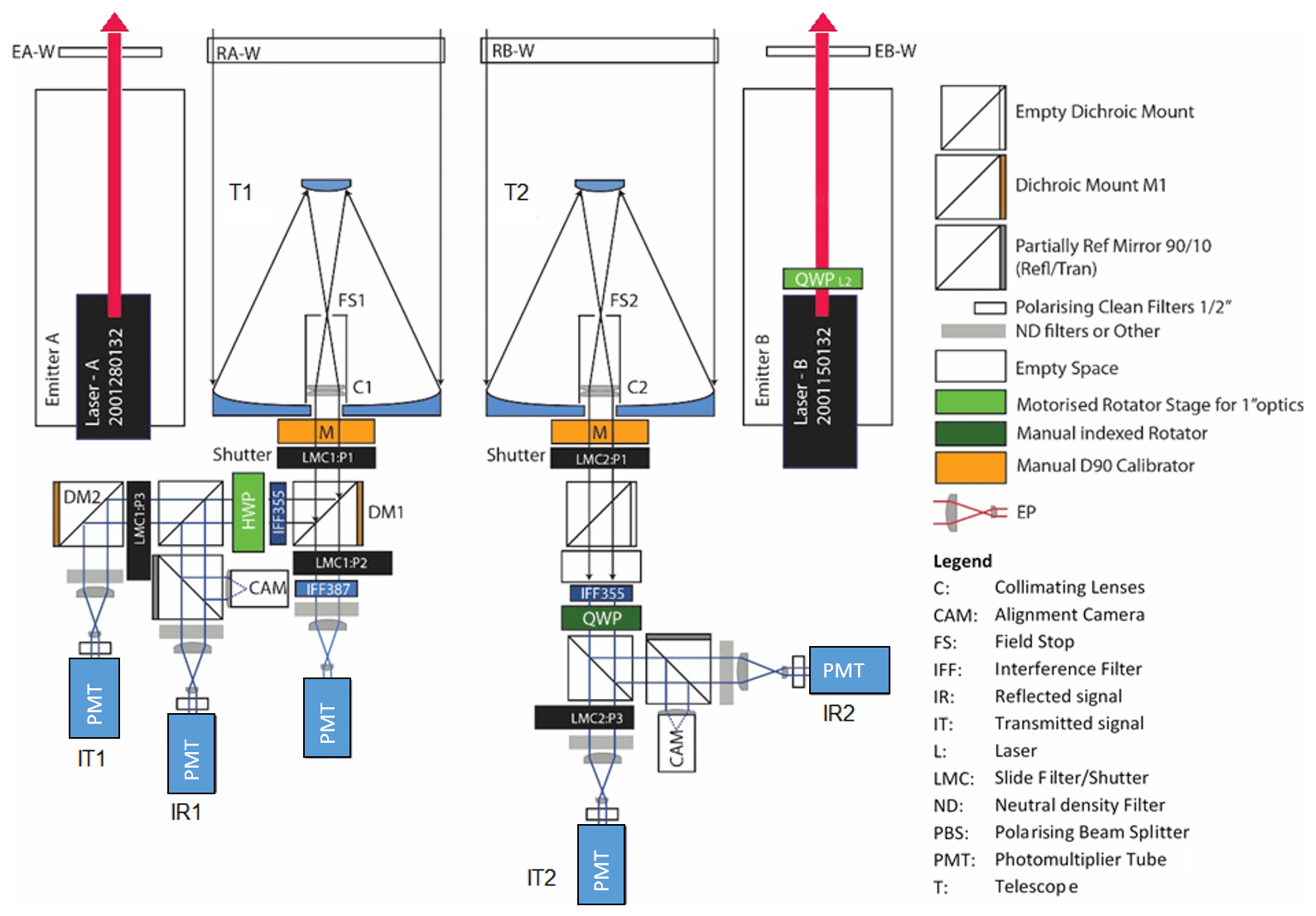
Figure 2Schematic of the lidar head. The two lasers A and B emit linearly and circularly polarised light, respectively, whereas the two telescopes 1 and 2 along with their receiver optics (i.e. the WSU1 and WSU2) collect the elastically and inelastically backscattered light and further analyse the linear and circular polarisation of the elastically backscattered light. The analysed signals are detected by five PMTs.
2.1.2 Detection
Each receiver unit consists of an afocal system composed by a telescope (T1, T2) and a collimating lens (C1, C2), and a proximate wavelength separation unit (WSU) (see Fig. 2). The two telescopes are Dall–Kirkham-type, designed and manufactured by Raymetrics S.A., utilising an elliptical prolate primary mirror and a spherical secondary mirror, with an aperture of 200 mm and focal length of 1000 mm (F no. 5). The afocal system has a reduction factor of about 13.5; thus the diameter of the received backscattered light beam is around 15 mm after the collimating lens and before the beam reaches the WSU. One field stop in each receiver (FS1, FS2) is used for determining the field of view (FOV) of each receiver. The field stops are graduated ring-actuated iris diaphragms with minimum apertures of 1 mm and maximum of 12 mm. Currently, the iris diameters are set to 2 mm, resulting in a FOV of 2 mrad full width, achieving a good sky background light suppression and a full overlap range at 400 m (see Appendix B).
Each WSU is mounted to its telescope on a manual rotator (M) that can rotate the whole WSU around the optical axis with a fixed step of 45∘ and continuously in a small range around the zero position in order to compensate for a mechanical misalignment with respect to the laser polarisation orientation. The manual rotator is used for calibration purposes (Sect. 3). Motorised shutters (LMC1:P1 and LMC2:P1) are placed behind the manual rotator in both WSUs to block the entrance of light in the WSU, facilitating the dark signal measurements.
In WSU1, the incoming collimated light passes through a dichroic long pass mirror (DM1), custom-made by Chroma Technology GmbH, transmitting wavelengths larger than the 365 nm and reflecting all smaller wavelengths. The transmitted light goes through an interference filter (IFF), custom-made by Alluxa Inc., with a central wavelength of 386.7 nm and width of 0.9 nm, in order to isolate the inelastic vibrational Raman backscattered light from atmospheric nitrogen, which is eventually collected by a PMT. An additional motorised shutter (LMC1:P2) is installed before the IFF, to protect the Raman PMT cathode from strong incident light during daytime. The reflected light goes through a 354.7 nm IFF (custom-made by Alluxa Inc.) with 0.5 nm width and a motorised rotating half-wave plate (HWP) before reaching the polarising beam splitter cube (PBS). The HWP is used for polarisation calibration purposes (see Sect. 3). The PBS is a UV fused silica beam splitter with anti-reflection coating in the range of 345–365 nm that separates the incoming light in two orthogonal polarisation components with respect to its eigenaxis. The transmission of p-pol (light polarised parallel to the incidence plane of the PBS) is 98.7 %, and the reflection of the s-pol (light polarised perpendicular to the incidence plane of the PBS) is 99.98 %. For linearly polarised emission, the PBS acts like a linear analyser and separates the parallel and cross-components of the backscattered light with respect to the original laser polarisation orientation in the reflected and transmitted paths of the PBS, respectively. Due to space restrictions, a second dichroic mirror (DM2) is placed in the transmitted path of the PBS, folding the transmitted light path from the PBS towards the PMT. Finally, the beam diameter of the reflected and transmitted light is further reduced to less than 4 mm using beam reducers (eye pieces; EPs) with a reduction factor of about 3.75, before being collected from the PMTs (an eye-piece is also placed before the Raman PMT). The eye pieces are used in order to avoid distortions in the recorded signals by the inhomogeneous detection sensitivity across the active area of the PMT's cathode (Freudenthaler, 2004; Freudenthaler et al., 2018; Simeonov et al., 1999).
In WSU2, the incoming light that initially passes through is a 354.7 nm IFF with 0.5 nm width. Before the PBS, a QWP is placed in a fixed position of 45∘ with respect to the PBS eigenaxis. The QWP along with the PBS acts as a circular analyser (Freudenthaler, 2016). For circularly polarised emission, a circular analyser separates the backscattered light to the co-polar and cross-polar components with respect to the original laser polarisation orientation in the reflected and transmitted paths of the PBS, respectively. The reflected and transmitted light from the PBS passes through the EP, and then it is collected from the cathode of the PMTs.
At both WSUs, cleaning polarising filters are placed before the PMTs. These filters reduce the crosstalk effect of the PBS, with a contrast ratio between the parallel and the perpendicular transmittance of 1000:1, and with this crosstalk cleaning, the PBS can be considered ideal (Freudenthaler, 2016). In addition, the reflected light from the PBS goes through a partially reflecting mirror, where ∼90 % of the light is reflected towards a camera (CAM) for system alignment purposes, while the rest is transmitted and detected by the PMT.
The transmitted optical paths, that correspond to the cross-polar component of the collected light in both WSUs, include a detachable filter on a motorised actuator (LMC1:P3 and LMC2:P3) that is deployed during the polarisation calibration measurements. Moreover, neutral density filters can be placed in front of each PMT in order to achieve optimum signal levels.
2.1.3 System alignment
The two lasers and the two telescopes are placed in a compact diamond-shaped layout, ensuring equal distances for both lasers to both telescopes and also facilitating the alignment of both lasers with each telescope at the same time. The system alignment can be achieved following a two-step procedure. In the first step, the two telescopes were co-aligned using a non-obscured target in the far range (e.g. a hill or a mountain top) and the two cameras (one for each telescope) in the receiver unit. The telescopes' co-alignment was achieved when both cameras could “see” the same far-range target by optimising the inclination of the secondary mirror with respect to the primary mirror for each telescope. This first step is expected to be performed occasionally if needed (e.g. after transportation of the lidar in a new site), rather than before each lidar measurement since due to the system's design there is no reason of misplacement of the secondary mirrors with respect to the primary mirrors of the telescopes from day-to-day operations.
The second and final step is about the co-alignment of the two lasers with the two telescopes. It is achieved by tilting each laser towards the co-aligned telescopes until both laser beams are well-aligned when inspecting the images from the two cameras. The second step is expected to be performed before each lidar measurement in case the images of the two cameras indicate a slight misalignment of the lasers with respect to the two telescopes.
2.2 The alt-azimuth positioner
The positioner consists of two side arms and a base along with a laser on indicating beacon, as is shown in Fig. 3. The base can rotate in azimuth, and a manual break is used to keep the head fixed at the desired azimuth direction. A large worm gear reducer is used to hold the position of the head at any zenith angle. Thus, the positioner provides a manual scanning capability to the lidar, since the lidar head can be rotated to point at different zenith and azimuth angles. Due to the umbilical tubes, the positioner enables the rotation along azimuth from −150 to +150∘ and the elevation from −10 to +90∘ off-zenith.
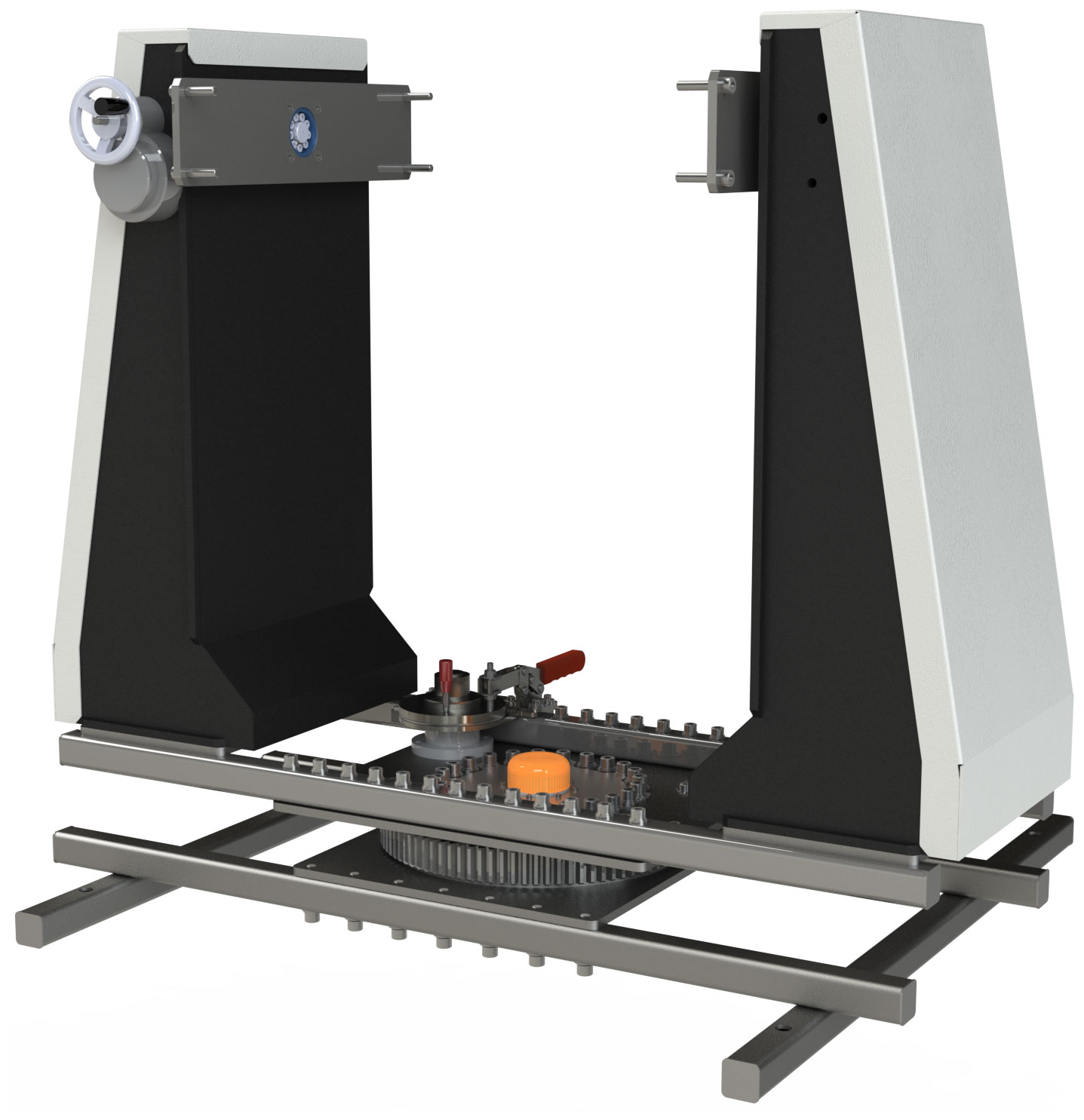
Figure 3The alt-azimuth positioner with its two side arms and the base.
2.3 The electronics enclosure
As shown in Fig. 4, the electronics enclosure contains a precipitation monitor, an external enclosure with DC power supplies, a dedicated lidar peripheral controller integrated with an industrial computer, two detection electronic racks (Licel GmbH), an online UPS, two power supplies and cooling units for the lasers, a fully programmable power distribution unit, two heat exchangers, the power cable along with the lidar's main switch, and two sockets for the umbilical tubes. The electronics enclosure is weather-protected, and its internal temperature is stabilised at 30±2.5 ∘C by the air to water heat exchangers.
The lidar peripheral controller is the unit that controls (locally or remotely) the lidar through several ethernet interfaces. In addition, the lidar peripheral controller is connected with several hardware interlocks, like the emergency button or a switch in the lidar head covers, for shutting down the lasers for safety reasons or in case of emergency.
Considering the two detection electronic racks (see Fig. 4), the first one contains the five transient recorders (TRs), along with the master trigger control unit, while the second one contains the five PMTs' high-voltage power suppliers. The TRs digitalise the PMT signals simultaneously in analogue and photon-counting mode, resulting in the acquisition of 10 signals composed by the four depolarisation channels plus one Raman channel in analogue and photon-counting mode. The demanding requirement of reaching the best dynamic range in the signal detection along with high temporal resolution under high repetition rates is fulfilled by means of an analogue-to-digital converter (ADC) of 16 bit at 40 MHz, developed by Licel GmbH (2020). The trigger control unit controls the two lasers and two receivers enabling the interleaved emission in order to avoid the interference between the pulses from both lasers and consequently the synchronisation of emission and acquisition. In detail, the trigger generator firstly triggers the laser LA to start emitting outgoing light pulses and all the TRs for the acquisition of the 10 backscattered signals (5 analogue and 5 photon-counting) of both telescopes in a memory slot A of the Licel transient recorders. Then, it triggers laser LB and all the TRs for the acquisition of the rest 10 backscattered signals in a memory slot B. For each laser, the trigger generator triggers the TRs to start recording prior to the triggering of the laser to emit laser pulses, resulting in an acquisition of only the background signal originating from the electronics and the solar background in the first recorded signal bins. This artificial region is the so-called pre-trigger region, which is used in the preprocessing of the recorded signals (see Sect. 4.1).
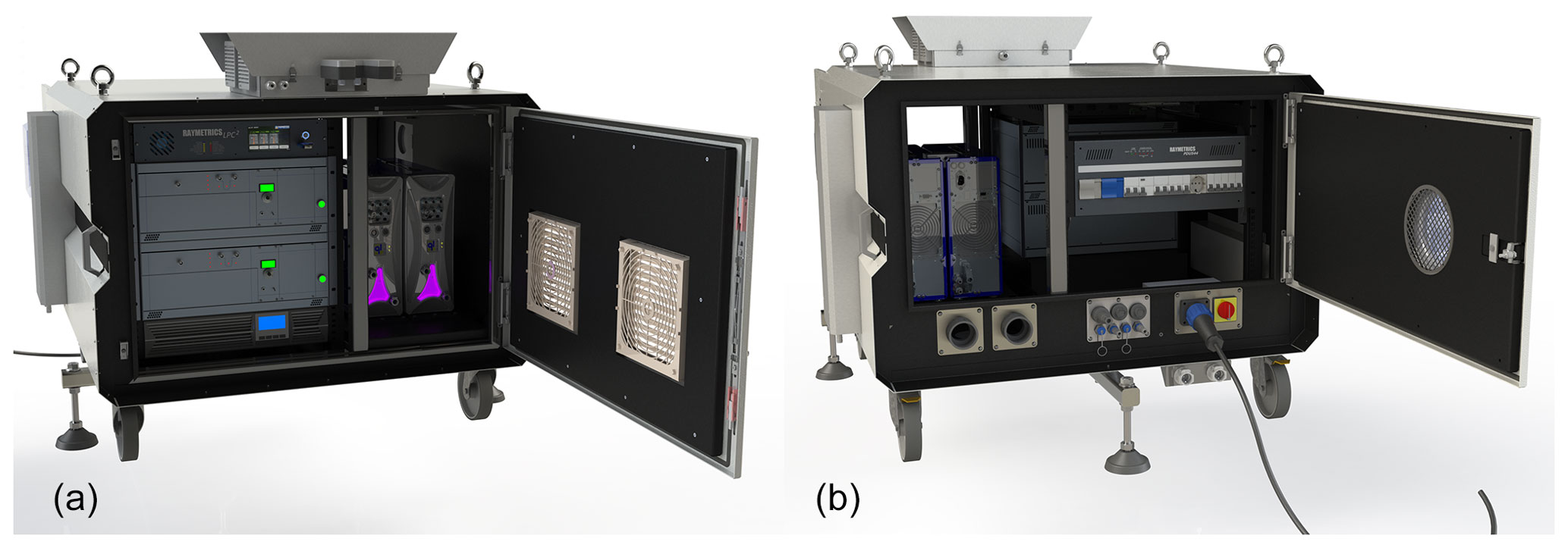
Figure 4The front (a) and back (b) view of the electronics enclosure.
A relative calibration of the depolarisation channels of the eVe lidar is required (Freudenthaler, 2016; Sassen, 2005). An extended description on how each lidar setup is handled for calibration purposes along with techniques for aligning the polarisation plane of the emission and the optical parts with respect to the reference plane as well as for diagnosing unwanted polarising effects will be given in a follow-up paper. Here, only the outcome of the applied calibration methods is provided. It has to be pointed out that for all applied methods, it is assumed that the calibration measurements are performed in atmospheric layers with randomly oriented particles/molecules because only for this case do we know the theoretical distribution of the backscatter signal intensity in the two polarisation detection channels and can apply the theoretical corrections described in Freudenthaler (2016).
The definition of the polarisation calibration methodology is facilitated with the use of the mathematical Stokes–Müller formalism for the description of the system (Chipman, 2009a). More specifically, the Stokes vectors are used to describe the polarisation state of the light (Chipman, 2009b), and the Müller matrices are used to describe how the atmosphere (van de Hulst, 1957; Mishchenko et al., 2002; Mishchenko and Hovenier, 1995) and any optical element (Lu and Chipman, 1996) can alter the polarisation state of the transmitted light. Consequently, the polarisation lidar signals from eVe can be modelled according to the Stokes–Müller formalism in order to derive the equations for the calculation of the polarisation calibration factor for each WSU.
As already mentioned in the previous section, the master trigger control unit triggers the two lasers to emit interleaved outgoing pulses, and the TRs record the received signals in a different memory slot per laser. Considering this, four emission-detection configurations are created, constituting the eVe lidar, a quadruple lidar system, which can also successfully validate itself when comparing the attenuated volume backscatter signal that can be detected simultaneously from the four lidar configurations. Consequently, the particle backscatter coefficient profile from the four lidar configurations can be compared in terms of the optical products' inter-comparison. Additionally, the particle extinction coefficient from two lidar configurations can be inter-compared since the Raman channel in WSU1 detects the inelastic backscattered signal from both lasers. The four emission-detection configurations (A1, A2, B1, and B2) that operate in parallel are presented in Fig. 5.
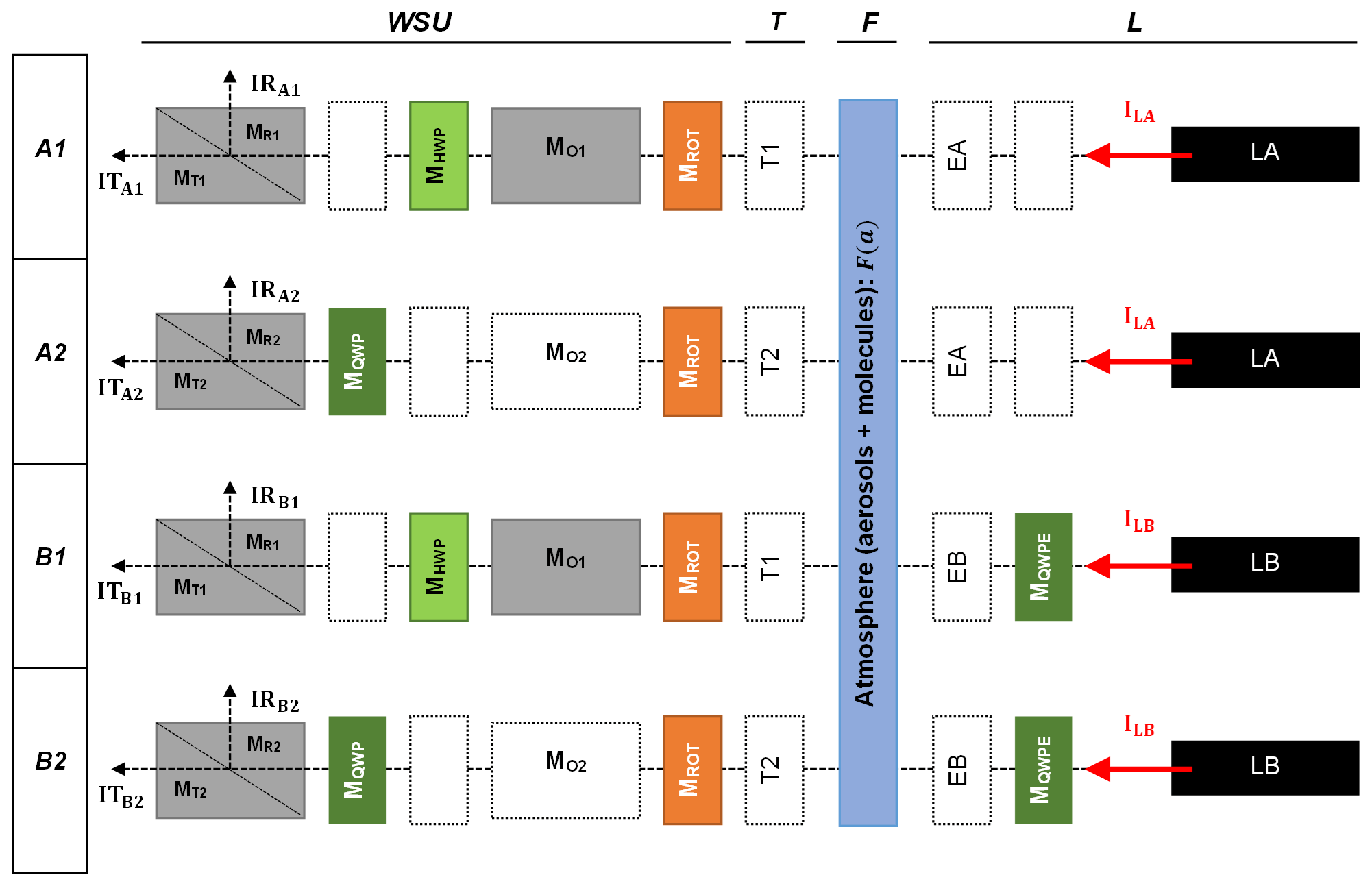
Figure 5Sketches of the four laser-receiver configurations that are formed with the interleaved measurements of the two-laser-two-telescope setup of eVe. A1 combines the linearly polarised emission of laser LA with the linear polarisation analyser WSU1. A2 combines the linearly polarised emission of LA with the circular polarisation analyser WSU2. B1 combines the circularly polarised emission of laser LB with the linear polarisation analyser WSU1. And finally, B2 combines the circularly polarised emission of laser LB with the circular polarisation analyser WSU2. See text for further details.
According to Fig. 5, the emission part (L) includes the Stokes vectors of the lasers (ILA and ILB) and the Müller matrix of the QWP in front of LB (MQWPE). The glass cover windows of the emitters A and B have been tested, and they do not introduce any significant polarising effects; thus they can be excluded from the Stokes–Müller formalism representation. Next in the optical path is the backscatter Müller matrix of the atmosphere (F(a), where is the atmospheric polarisation parameter; Chipman, 2009a; Freudenthaler, 2016). The telescope part (T1 and T2) contains the glass cover windows, the primary and secondary mirror, and the collimating lenses, which do not introduce polarising effects, and they can be excluded from the Stokes–Müller formalism representation. The collimating lenses are mounted in the telescope part with a stress-free method, and they have been checked for polarising effects with visual inspection techniques. The receiver part (WSU; wavelength separation unit) includes the Müller matrices of the manual rotator (MROT), the receiver optics, the motorised rotating HWP (MHWP) in WSU1, the QWP (MQWP) in WSU2 that is part of the circular analyser, and the PBS including their cleaning polarisation filters for the reflected and the transmitted channels (MR1, MT1 and MR2, MT2). After the PBS, the corresponding Stokes vectors of the light in the reflected and transmitted path of the PBS are given (IRij and ITij, respectively, where and considering the four lidar configurations.
The laser emission at 355 nm is highly polarised with a degree of linear polarisation (DOLP) of 0.997 and 0.998 for LA and LB, respectively, which has been measured in the laboratory by a custom-made laser ellipsometer (LEM) suitable for high-power lasers. In the LEM, the laser light is attenuated and then enters a depolarisation splitting compartment, almost identical to the one which is included in the eVe's WSUs. Regarding the receiver optics, the only part that could introduce diattenuation or retardance is the dichroic beam splitter in WSU1 (MO1). According to Freudenthaler (2016), it can be modelled as a non-rotated retarding diattenuator because the eigenaxis of the dichroic beam splitter is well aligned with the PBS eigenaxis. The cleaned PBS and all waveplates are considered ideal, and their expressions for a given rotation angle can also be found in Freudenthaler (2016). On the other hand, the receiver optics in WSU2 includes the IFF, which is not expected to change the state of polarisation and is excluded from the Stokes–Müller formalism representation since it is placed into the WSU2 with a stress-free method. More specifically, all the IFFs used are mounted on aluminium rings from the manufacturer, and stress-free retaining rings (O-ring) are used for fixing the mounted IFFs into the WSUs. In addition, the PBS incidence plane of the respective WSU is selected as the polarisation reference plane, and all rotational optical parts (QWPE, HWP, and QWP) are accurately aligned by means of rotation mounts with respect to this plane. The rotation mounts for the QWPE and HWP are motorised with a minimum incremental motion of 0.001∘ and a bidirectional repeatability of 0.003∘. The rotation mount for the QWP in the circular analyser of WSU2 enables only a manual rotation; thus the position of the QWP is fixed at 45∘ with respect to the PBS eigen axis.
The alignment of the polarisation plane of the emitters with the reference plane is also necessary, at least for the linearly polarised emission with respect to the linear analyser in WSU1, since the circularly polarised emission and the circular analyser in WSU2 are independent of rotation. For that reason, the manual rotator in the WSU1 can be used to align the emitter A with the WSU1 according to Freudenthaler (2016) Sect. 11.
The configurations A1 and B2 are used to obtain the volume linear and volume circular depolarisation ratios, respectively, as well as the backscatter and extinction coefficients from the two polarised emissions, while the other two configurations, A2 and B1, are used for calibration purposes and also to diagnose unwanted polarising effects in the system.
3.1 Calibration factor in WSU1
When normal measurements are performed with configuration A1, the parallel and cross-polarised components are detected in the reflected and transmitted optical paths of the linear analyser, respectively, because the angle between the polarisation plane of the laser and the eigenaxis of the PBS is 90∘ (Freudenthaler et al., 2009). According to Freudenthaler et al. (2009), this 90∘ difference can reduce the crosstalk errors even more due to higher reflectance of the reflected path of the PBS with respect to the transmittance of the transmitted path of the PBS, which is also the case for eVe (see Sect. 2.1.2). Additionally, the cleaning polarising filters that are placed before the PMTs in the reflected and transmitted optical paths of each PBS eliminate the crosstalk errors, and thus the PBS is considered ideal (Freudenthaler, 2016). The calibrated signal ratio of the reflected and transmitted channels, which is defined in Freudenthaler (2016; Eq. 60) can be written as
where η1 is the calibration factor that corresponds to the relative amplification of the reflected (IR,A1) and the transmitted (IT,A1) channels in WSU1, DO1 is the diattenuation parameter of the receiver optics (Freudenthaler, 2016; Sect. S.4 in the Supplement), and is the volume linear depolarisation ratio of the atmosphere. Once the calibration factor and the diattenuation parameter of the receiver optics are determined, the volume linear depolarisation ratio can be retrieved.
The calibration factor (η1_HWP) is determined with configuration A1 by means of the Δ90 calibration method using the HWP in front of the PBS (Freudenthaler, 2016; Sect. 7.1). It does not include the polarisation effects of optical parts before the HWP. That is why the correction for the diattenuation in Eq. (1) is necessary. The calibration measurements are performed by rotating the HWP at ±22.5∘ with respect to its zero position, which corresponds to the rotation of the linear polarisation orientation of the incident light by ±45∘ with respect to the PBS incidence plane. The calibration factor (η1) that is calculated from the geometrical mean of the two gain ratios ( (±45∘)) of the calibration signals (Δ90 calibration) is independent of a rotational offset of the HWP (Freudenthaler, 2016; Eq. 105):
The diattenuation effect of the receiver optics (DO1) can be determined by performing an additional Δ90 calibration using the manual rotator of the WSU1 before the receiver optics at ±45∘ (Belegante et al., 2018; Freudenthaler, 2016), which yields the calibration factor η1_manual. From the ratio of the two calibration factors, we can retrieve the diattenuation parameter of the receiver optics (DO1) using Eq. (3) (Belegante et al., 2018; Freudenthaler, 2016):
With this technique, DO1 was found to be 0.000±0.011.
Upon the determination of DO1, the calibration factor can also be calculated using the configuration B1 by performing directly normal measurements, i.e. without any rotation of the calibrators. It has to be pointed out that this calibration procedure can be applied only in case the receiver optics does not produce retardation effects, which has to be verified first. The gain ratio ( of the measured reflected and transmitted signals from B1 (IR,B1 and IT,B1) is identical to ηA1.
3.2 Calibration factor in WSU2
When normal measurements are performed with configuration B2, the co- and cross-polar components of the backscattered signal are detected in the reflected and transmitted optical paths of the circular analyser, respectively, like in configuration A1 above. The calibrated signal ratio of the reflected and transmitted channels can be written as
where η2 is the relative calibration factor between the reflected (IR,B2) and transmitted (IT,B2) channels in WSU2, and is the volume circular depolarisation ratio. Once the calibration factor is determined, the volume circular depolarisation ratio can be directly calculated.
Here, the calibration factor can be easily determined with any combination of linear and unpolarised light, regardless of the rotational angle of the linearly polarised component. The linearly polarised light after passing through the QWP is converted to elliptically polarised light and can be expressed as a combination of circularly and linearly polarised components. It can be proven that the linearly polarised component is either parallel or perpendicular to the eigenaxis of the QWP. Since the QWP is placed at 45∘ with respect to the PBS, the linearly polarised component is split in half. Any combination of unpolarised and circularly polarised light is also split in half by the PBS in WSU2. Thus, the configuration A2 can be used directly, without any adjustment, for the determination of the calibration factor η2. As there is no polarising optical element before the circular analyser in WSU2 that has to be considered for normal measurements, the gain ratio ( of the measured signals is equal to the calibration factor (η2) in Eq. (5).
Configuration B2 can be used in the same way for the determination of the calibration factor η2, by adjusting the motorised QWPE after the laser LB so that it is at 0∘ with respect to the original linear polarisation of laser LB, resulting in the emission of linearly polarised light from emitter B.
Processing software has been developed for the analysis of the recorded signals and the corresponding retrieval of the optical products. The software relies on well-known equations for the lidar signal processing and the lidar products' retrieval that are also applied in the existing lidar processing algorithms such as the software of PollyNET (Baars et al., 2016) and the Single Calculus Chain (D'Amico et al., 2016; Mattis et al., 2016), as well as the algorithms used individually by stations within EARLINET (Böckmann et al., 2004; Pappalardo et al., 2004). Each piece of software has its own workflow and may apply different approaches regarding the signal processing (e.g. the type of the filter for signal smoothing). As such, this section presents the workflow of the developed software for the processing of the lidar signals as well as the basic equations that are used in the retrieval of the optical products.
The required inputs are raw lidar signals and ancillary information regarding the lidar configuration (location's coordinates and measurement zenith and azimuth angles) and the atmospheric conditions (temperature, pressure, and humidity height profiles) under which the measurements were performed. The retrieved aerosol optical products are the height profiles of the particle backscatter coefficient, the particle extinction coefficient, the lidar ratio (extinction-to-backscatter ratio), and the volume and particle linear depolarisation ratios, as well as the volume and particle circular depolarisation ratios at 355 nm. The software is divided in two modules, i.e. the preprocessing chain and the aerosol optical product processing chain. In addition, the software is capable of analysing signals from the dark measurements (Freudenthaler et al., 2018) and during quality assurance and quality control tests proposed by EARLINET, such as the telecover test, the Rayleigh-fit test, and the polarisation calibration (Freudenthaler et al., 2018).
4.1 Preprocessing chain
The preprocessing chain handles the raw signals which will be used for the retrieval of the aerosol optical products. Since the raw lidar signals are recorded in both photon-counting and analogue modes, the following corrections are applied. First of all, the photon-counting signals are corrected for the dead time introduced by the PMT and the photon counter electronics (Donovan et al., 1993; Evans, 1955). Then, in order to increase the signal-to-noise ratio (SNR), the signals are averaged in time, using a time window that is also representative of the corresponding atmospheric conditions. After time averaging, the atmospheric background that corresponds to an offset value is subtracted from the signals. The background signal introduced by the electronics in analogue detections is subtracted from the corresponding analogue signals as well. The pre-trigger region is preferred for the calculation of the background offset value in order to avoid the small but not negligible contribution of the atmospheric backscatter at the far end of the signal. The pre-trigger region is then corrected for the signals by the first bins that correspond to the pre-trigger region and contain only the background signal, considering the correct trigger delay between the outgoing laser pulse and the actual TR start time, which can be determined according to the trigger delay test in Freudenthaler et al. (2018). To further increase the SNR, the signals are vertically smoothed by means of a polynomial fit with the capabilities of defining the polynomial order and the length of the smoothing window, which can be fixed (see D'Amico et al., 2016) or variable (see Ansmann et al., 1992; Wandinger and Ansmann, 2002).
After the vertical smoothing, the analogue and photon-counting signals per channel are “glued” in a range that both signals are not distorted in order to produce a combined signal with increased dynamic range compared to the individual ones (Mielke, 2005). Eventually the “range-corrected” signals are corrected for the range dependence of the recorded signal profile (Weitkamp, 2005). In addition, the algorithm is capable of applying a correction in the signals for incomplete overlap. The overlap profile can be obtained following the methodology proposed by Wandinger and Ansmann (2002), which is restricted by the assumption of temporal and vertical homogeneity of the suspended aerosols below the full overlap height. In the case of the eVe lidar, which has manual scanning capabilities in terms of pointing the lidar head at different azimuth and off-zenith angles for a measurement rather than performing 3-dimensional scanning lidar measurements (Behrendt et al., 2011; Pal et al., 2006), a sensitivity study must be performed on the overlap function in order to investigate whether it is stable over time and over all the pointing measurement angles. This sensitivity study has not been conducted yet; thus the processed signals are not overlap corrected. However, during the lidar operations only small misalignment issues have been observed with changes of the pointing geometry. Hence, the system alignment is checked before each measurement by visual inspection of the alignment cameras and/or by performing a telecover test, and, if needed, the second step of the system alignment procedure (see Sect. 2.1.3) is performed in order to refine the alignment and achieve the full overlap range of 400 m (see Sect. 2.1.2).
For each WSU, the preprocessed corrected signals from the co-polar and cross-polar components are combined to construct a new signal, defined as the calibrated sum of the respective polarised components according to Freudenthaler (2016; Eq. 65). The calibrated sum signal is proportional to the total signal that would have been recorded if the beam had not been split with the PBS.
In analogue signals, the electronic noise can produce range-dependent artefacts that cannot be removed through the background subtraction from the signal (Freudenthaler et al., 2018). The processed analogue signals can be corrected from these range-dependent artefacts using the signals acquired from a dark measurement, which is performed with fully covered telescopes before each normal measurement. The same processing procedure is applied in the dark measurement signals, and then they are subtracted from the normal measurement signals.
4.2 Optical product processing chain
In the aerosol optical product processing chain, the desired optical products are retrieved using the preprocessed lidar signals. Before the retrieval of the optical products, the profiles of the nitrogen molecule number density and of the molecular backscatter and extinction coefficients are calculated using the temperature and pressure profiles and the appropriate conversion factors (Freudenthaler et al., 2018). The temperature and pressure profiles are acquired from the nearest launched radiosonde or from a numerical weather prediction model (NWP); if none is available, a standard atmospheric model (e.g. the U.S. Standard Atmosphere) is used instead, adapted to the surface temperature and pressure values at the measurement site. Finally, the range-corrected signal profiles (I(z)) along with the theoretical molecular profiles (N(z), βm(z), αm(z)) are used for the retrieval of the following optical properties.
4.2.1 Particle extinction coefficient
The particle extinction coefficient (αp) profile is retrieved according to the Raman inversion method using the signal that is inelastically backscattered by nitrogen molecules (Ansmann et al., 1992):
where z is the range (i.e. distance from lidar), I(z,λRA) is the inelastic range-corrected signal, N(z,λRA) is the nitrogen molecule number density, αm(z,λ0) is the molecular extinction coefficient at the laser wavelength λ0, αm(z,λRA) is the molecular extinction coefficient at the Raman wavelength λRA, and k is the Ångstrom exponent which is assumed to be known (ideally the value is taken from nearby AERONET measurements). According to Ansmann et al. (1992), a deviation of the Ångstrom exponent from its true value in the order of 1 can cause a relative error of less than 4 % in the retrieval. The particle extinction coefficient is a night-time-only product as daylight hinders the detection of the weak Raman signal. The Raman channel can record Raman backscattered signals from both lasers; thus the extinction coefficient of both linearly and circularly polarised emitted light can be calculated independently.
4.2.2 Particle backscatter coefficient
The Raman inversion method (Ansmann et al., 1992) can also be used for night-time measurements to retrieve the particle backscatter coefficient (βp) profile using both the elastic and inelastic backscatter range-corrected signals, I(z,λ0) and I(z,λRA), respectively.
where βm(z,λ0) is the molecular backscatter coefficient profile at range z, and βm(z0,λ0) is the value of the molecular backscatter coefficient at the reference range z0. The reference range is an aerosol-free region, which is selected manually by visually inspecting the Rayleigh fit (Freudenthaler et al., 2018) between the preprocessed signals and the attenuated molecular backscatter coefficient.
In absence of inelastic backscatter signals, as for example for daytime conditions, the particle backscatter coefficient is obtained with the Klett–Fernald–Sassano (hereafter Klett) inversion method (Fernald, 1984; Klett, 1981; Sasano and Nakane, 1984) using only the elastic backscatter signals. The inversion assumes a height constant particle lidar ratio Lp and a priori knowledge of the backscatter coefficient β(z0,λ) at the reference range z0. Under these assumptions, the lidar equation for elastic backscatter signals can be solved by means of boundary conditions if handled like a differential Bernoulli equation. The solution of the total backscattering coefficient at a wavelength λ can be written as
where Lm is the molecular lidar ratio.
4.2.3 Volume depolarisation ratios
According to Freudenthaler (2016) the calibrated signal ratio (δ∗) of the reflected (R) and transmitted (T) channels of an analyser (linear or circular) can be expressed as a function of the height-dependent atmospheric polarisation parameter a and the constant system parameters GS and HS (:
The GS and HS parameters are used to describe the polarisation crosstalk effects in the system that depend on the state of the laser polarisation and on the diattenuation and/or retardation of the optical elements in both the emission and receiver units, as well as their relative rotation with respect to the reference plane. As a result, the GS and HS parameters differ for each one of the four configurations of eVe. The K parameter is also introduced by Freudenthaler (2016; Eq. 83), for the theoretical correction of the measured calibration factor that is determined with a non-ideal lidar system by means of the Δ90 calibration or similar, in order to retrieve the calibration factor η. In the case of eVe lidar where “cleaned” analysers are used (cleaning polarising filters after the PBS), the K parameter is equal to one.
The polarisation parameter a can be retrieved from Eq. (9):
According to Mishchenko and Hovenier (1995), the polarisation parameter a ( therein) is the sole parameter of the backscatter matrix of an atmospheric scattering volume consisting of arbitrary shaped particles and their mirror particles in random orientation that fully describes the polarisation property of matrix. The linear and circular depolarisation ratios and their theoretical relationship for these conditions can be expressed as a function of the polarisation parameter (Eqs. A12 and A13) (Mishchenko and Hovenier, 1995).
The volume linear depolarisation ratio is retrieved through Eq. (A12) using the calibrated signal ratio of the A1 configuration ( from Eq. (1) and the polarisation parameter a from Eq. (10):
The volume circular depolarisation ratio is retrieved through Eq. (A13) using the calibrated signal ratio of the B2 configuration ( from Eq. (4) and the polarisation parameter a from Eq. (10):
4.2.4 Particle depolarisation ratios
According to Beyerle (1994), the particle linear depolarisation ratio profile can be calculated from the following equation where :
and using the profiles of the volume linear depolarisation ratio ( and the total backscatter to molecular backscatter ratio (scattering ratio; R) and the molecular linear depolarisation ratio value (. Equation (13) can also be used for the calculation of the particle circular depolarisation ratio profile using the volume and molecular circular depolarisation ratios instead ( and and assuming a circular polarisation in the methodology of Beyerle (1994).
4.3 Statistical uncertainty estimation
The estimation of statistical uncertainty of each retrieved optical product from the software is based on the Monte Carlo simulations (Robert and Casella, 2010). The Monte Carlo method consists of repeated retrievals, each time varying the input data (lidar signals) randomly within their stated limits of precision. If a realistic error can be simulated for the input data, then, the final optical product error distribution and standard error can be estimated. A benefit of this technique is that no assumptions are required during error propagation (e.g. assuming uncorrelated errors). A more detailed description on the application of the Monte Carlo method in the calculation of the statistical uncertainty in the retrieved products is given in D'Amico et al. (2016) and Mattis et al. (2016).
4.4 Algorithm inter-comparison
The algorithms for the processing of the lidar data have been tested using the synthetic lidar dataset which has been created for the algorithm inter-comparison exercise performed in the framework of EARLINET (Böckmann et al., 2004; Pappalardo et al., 2004). In brief, the dataset contains a 30 min time series of synthetic raw lidar signals simulated assuming realistic experimental and atmospheric conditions. The temperature, pressure, extinction coefficient, backscatter coefficient, and lidar ratio profiles that were used as an input for the simulation of the synthetic signals are provided in Fig. 2 in Pappalardo et al. (2004). It has to pointed out that the corresponding aerosol optical depth (AOD) for the simulated atmospheric scene is 0.82 at 355 nm and 0.45 at 532 nm, representing a rather heavy aerosol load in the atmosphere compared to measured AOD time series over different regions (e.g. Baars et al., 2016; Giannakaki et al., 2015; Voudouri et al., 2020). Both elastic (at 355 nm) and N2 Raman (at 387 nm) raw lidar signals are taken into account to reproduce a real measurement sample of a typical advanced multi-wavelength Raman lidar as much as possible, with an incomplete overlap between the laser and the receiver field of view below 300 m. The synthetic signals were processed with the developed software for eVe products (eVe software) and are shown in Fig. 6, where a vertical smoothing with a first-order polynomial fit and a smoothing window of 100 m was applied. In addition, the signals were not corrected for the incomplete overlap, and the reference height of molecular region was selected at 6.5 km altitude within a 0.5 km window.
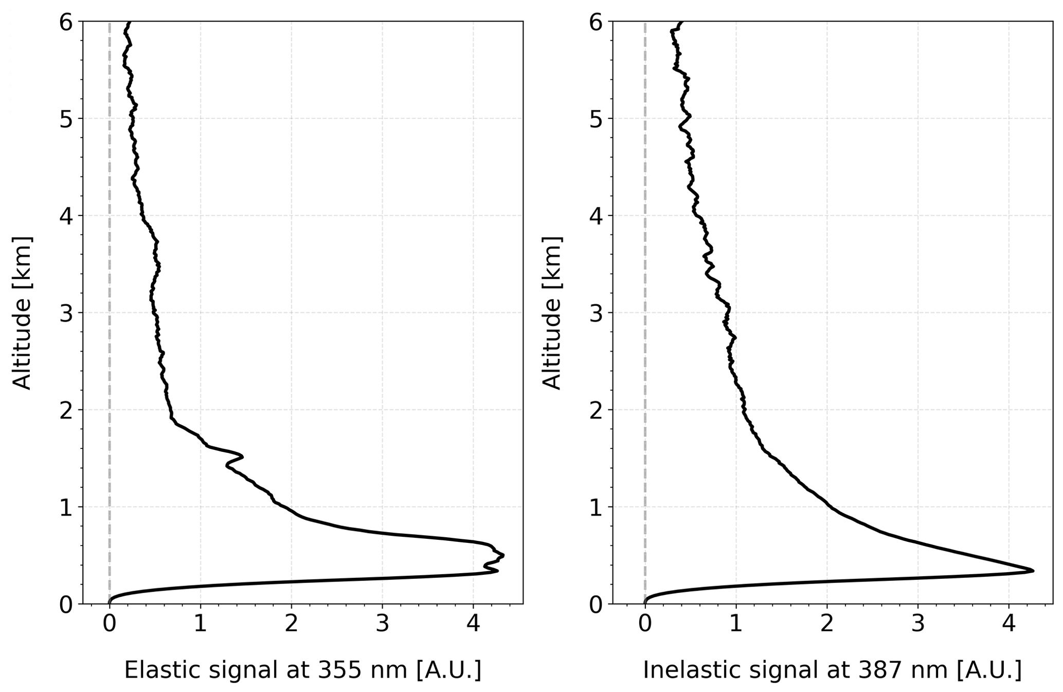
Figure 6The synthetic elastic and inelastic signal profiles at 355 and 387 nm, respectively, that were used as an input in the eVe software. The signals are range-corrected and vertically smoothed with a first-order polynomial fit and a smoothing window of 100 m.
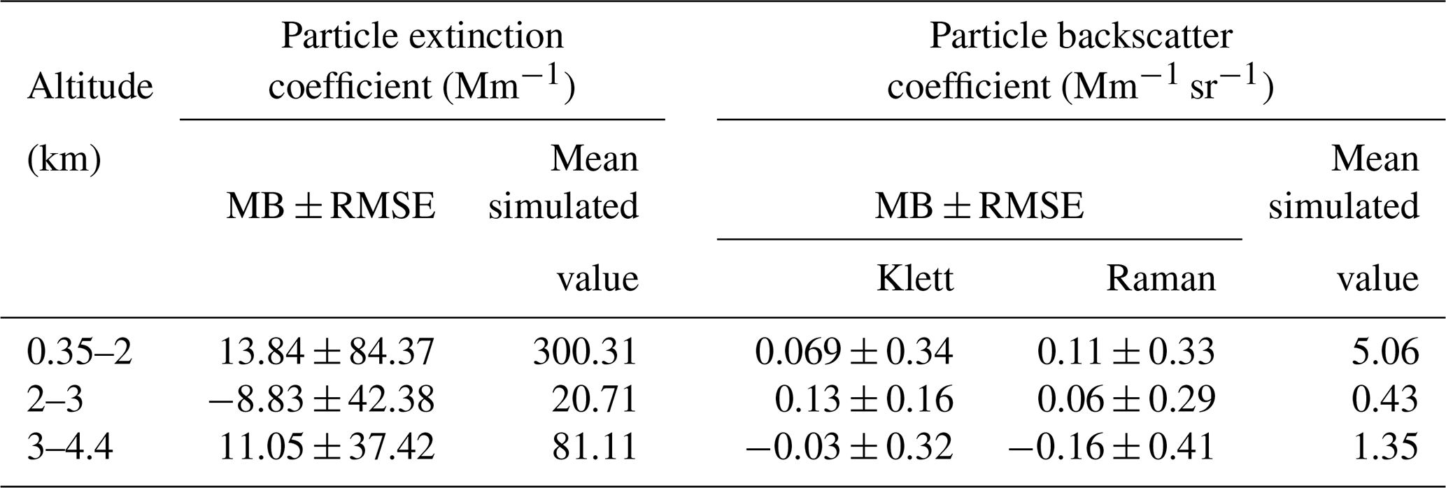
The particle backscatter and extinction coefficients at 355 nm were retrieved using the eVe software and the simulated synthetic signals as input to the software. The backscatter coefficient was retrieved using both the Raman and the Klett inversion methods, where for the latter, a height-constant aerosol lidar ratio of 60 sr, which is known a priori from the simulation, was used. The retrieved profiles (from eVe software) of the backscatter and extinction coefficients are compared with the respective profiles of the backscatter and extinction coefficients that were used for the signals' simulation (simulated). Figure 7 shows the inter-comparison between the simulated and the retrieved coefficients. For the statistical analysis of the inter-comparison, the bias was calculated as the difference between the simulated and the retrieved profile using the simulated profile as reference. The mean bias and the respective standard error were calculated inside three selected altitude regions from Pappalardo et al. (2004) and are provided in Table 1 for both the particle extinction and the backscatter coefficients. The first region extends from 0.35 to 2 km, representing typical aerosol load inside the planetary boundary layer, the second region that is aerosol-free extends from 2 to 3 km, and the third region extends from 3 to 4.4 km, where an elevated aerosol layer is present.
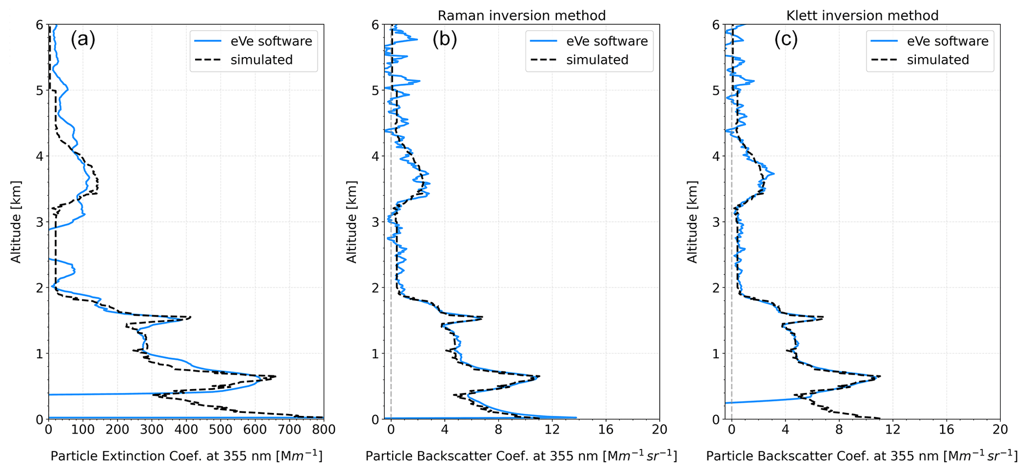
Figure 7Comparison of the extinction coefficient profile (a) and the backscatter coefficient (b and c) at 355 nm retrieved from the eVe software (solid; blue) and the simulated profile (dashed; black). The backscatter profile was retrieved using both the Klett (b) and the Raman (c) inversion method, where the reference height for Rayleigh atmosphere was selected at 6.5 km with a 0.5 km window.
In Fig. 7a, below 0.35 km the retrieved profile of extinction coefficient is affected by the incomplete overlap that is present in the processed synthetic signals, and the retrieval inside this range region will be not taken into consideration for the inter-comparison. Overall, the retrieved extinction coefficient profile shows a good agreement with the simulated profile. In the first height range (0.35–2 km) the mean bias between the retrieved and the simulated extinction profile is 13.84 Mm−1, falling within the 23 Mm−1 that was found for the majority of the stations in Pappalardo et al. (2004). In the elevated aerosol layer (3–4.4 km) the mean bias is 11.05 Mm−1 and agrees well with the bias of 13 Mm−1 that was found in the majority of the stations in Pappalardo et al. (2004). In the aerosol-free height range (2–3 km) the mean bias is −8.83 Mm−1, denoting a trend of underestimation with respect to the majority of the stations in Pappalardo et al. (2004), where the bias is below 17 Mm−1, and 45 % of the stations have underestimation trends.
In the height range from 2 to 3 km, the retrieval is noisier, leading to an inaccurate representation of the molecular region. The combination of the weak and noisy Raman signal along with the low extinction values due to the molecular region can cause distortions in the differentiation in Eq. (6); the distortions can be further enhanced or removed depending on the selected derivative window for the differentiation. The artificial noise that was inserted in the synthetic signals (Fig. 6) was customised to simulate the higher levels of noise from older lidar signal recorders compared to the ones deployed on eVe. Hence, in such altitudes ranges, the lidar signals from eVe have a better SNR compared to the synthetic signals, resulting in a less noisy as well as more reliable retrieval of the extinction coefficient profile.
Table 1Mean bias (MB) and root mean square error (RMSE) of the particle extinction and backscatter coefficients for three altitude ranges. The mean value of the simulated particle extinction and backscatter coefficient profiles inside the three altitude ranges is also provided.
The backscatter coefficient profiles retrieved from both inversion methods, compared to the simulated one, show a rather good agreement, consistent with the most EARLINET algorithms in all altitude ranges, as shown in Fig. 7b and c. In the first height range (0.35–2 km) in Table 1 the mean bias for the Klett solution is 0.069 Mm−1 sr−1 and for the Raman solution is 0.11 Mm−1 sr−1 when the bias for most of the stations in Pappalardo et al. (2004) is below 0.54 Mm−1 sr−1 in absolute values. In the elevated aerosol layer (3–4.4 km) the retrieved profile seems to be underestimated with respect to the simulated profile, with the mean bias for the Klett and Raman solutions calculated to be −0.03 and −0.16 Mm−1 sr−1, respectively, falling well within the mean bias of −0.40 Mm−1 sr−1 that is found in most of the rest inter-comparison stations. Last but not least, in the aerosol-free region (2–3 km) the mean bias for the Klett and Raman solutions is 0.13 and 0.06 Mm−1 sr−1, respectively, while for the majority of the inter-comparison stations the mean bias is below 0.30 Mm−1 sr−1 in absolute values.
Below 0.3 km where the full overlap height is defined, the underestimation of the Klett solution with respect to the Raman solution is highlighted, since with the Raman method a backscatter coefficient profile can be obtained without the dependence of the overlap function as it is cancelled out in the ratio of the lidar signals in Eq. (7).
Overall, the profile from the Klett solution shows better agreement with the simulated one, compared to the noisier profile obtained from the Raman solution. In principle, the Raman solution is expected to be noisier, since the elastic and inelastic signals that are used bring two different uncertainties into the retrieval, while only the elastic signal is used for the Klett solution. On the other hand, the Klett solution strongly depends on the user-defined value of lidar ratio as well as on the given value of scattering ratio in the reference height of the molecular atmosphere. For the inter-comparison, the lidar ratio value of 60 sr, which was used in the eVe software for the Klett solution, was selected by inspecting the lidar ratio profile that was used as input for the signals' simulation (see Fig. 2 in Pappalardo et al., 2004), resulting in an optimum retrieval of the backscatter coefficient profile. Thus, if an inaccurate lidar ratio was used instead, the retrieved profile would deviate more from the simulated one.
Two selected measurement cases are presented from the first conducted measurements of eVe lidar. The system was located in Athens, Greece (38.06∘ N, 23.75∘ E), at an elevation of 194 m above sea level. For each case, a vertical smoothing with a first-order polynomial fit and a smoothing window of 100 m was applied in the measured signals. Moreover, the signals were not corrected for the incomplete overlap. The molecular profiles (N(z), βm(z), and αm(z)) that are needed for the products' retrieval were calculated using the temperature and pressure profiles acquired from launched routine meteorological radiosondes in Athens. The temperature profile was also used in order to calculate the molecular linear and circular depolarisation ratios that are expected to be measured from the lidar in aerosol-free regions. The expected molecular linear–circular depolarisation ratio profiles (mLDR and mCDR) have been calculated theoretically (Freudenthaler et al., 2018; Wandinger, 2005) by taking into account the temperature profile, the laser wavelength, and the specifications of the two IFFs at 355 nm (one in WSU1 and the other in WSU2), such as the central wavelength and transmission curve. Equation (A14) from Appendix A was used to derive the mCDR profile using the calculated mLDR profile for the used IFF at 355 nm in WSU2 (circular analyser). For the dates of the selected cases, the temperature ranges from −10 to 20 ∘C up to 5.5 km altitude height, resulting in a mean molecular linear depolarisation ratio of 0.00586±0.00004 and a mean molecular circular depolarisation ratio of 0.0119±0.00009. The retrieved optical products are the particle backscatter coefficient, the particle extinction coefficient, the lidar ratio, the volume and particle linear depolarisation ratios (VLDR and PLDR), and the volume and particle circular depolarisation ratios (VCDR and PCDR) at 355 nm. Aiming at a less noisy particle extinction coefficient retrieval, the derivative of the signal ratio (see Eq. 6) was calculated using different derivative windows within four signal range nodes. More specifically, in the first signal range node (up to 1.5 km) the derivative window was 200 m, in the second signal range node (from 1.5 to 4 km) the derivative window was 400 m, in the third signal range node (from 4 to 6 km) the derivative window was 600 m, and finally in the fourth signal range node (from 6 km to the end of signal) the derivative window was 800 m. The retrieved VLDR and PLDR were used in order to reproduce the VCDR and PCDR, respectively, using the theoretical relationship between them for randomly oriented particles (; Mishchenko and Hovenier, 1995; Roy and Roy, 2008). The comparison of the retrieved VCDR and PCDR with the converted ones (i.e. the VLDR-to-VCDR and the PLDR-to-PCDR) can indicate particle orientation and/or multiple scattering in case the retrieved profiles deviate from the converted ones (see Appendix A). In Appendix A we examined whether the theoretical relationship between the linear and the circular depolarisation ratios can be used with the backscatter coefficient retrieved from ground-based polarisation lidar systems to retrieve a product that is comparable with the Aeolus backscatter coefficient for the validation of the Aeolus L2A products. Hence, the “Aeolus-like” backscatter coefficient was calculated using the particle backscatter coefficient retrieved from the circularly polarised emission and Eq. (A15) from Appendix A. In this study, the Aeolus-like backscatter coefficient corresponds to the particle backscatter coefficient that Aeolus would measure from the ground.
5.1 Case study of 29 September 2020
Figure 8 gives an overview of the performed measurements on 29 September 2020, from 16:37 to 17:39 UTC. Traces of low clouds are present at approximately 3 km, between 16:37 and 16:48 UTC, and around 17:10 UTC at both attenuated volume backscatter signal and VLDR profiles. In addition, a very thin depolarising layer can be observed in the scene, through the VLDR profile, initially located at 3 km and then, as time passes, at approximately 2.6 km. Elevated layers with depolarising particles are present in the scene, at approximately 6.5 and 9 km. Moreover, depolarising particles are also detected inside the planetary boundary layer (PBL) (below 1 km), but they do not form a persistent layer, due to turbulent mixing at the surface caused by strong winds and convection on that day. These particles in the lower heights may originate from a local dust emission from industrial activities near the location where the lidar was placed, from the anthropogenic pollution of the Athens metropolitan area, and/or from the sea (marine aerosols). In addition, the depolarising particles at higher altitude ranges (above the PBL) may be traces of desert dust particles with very low values of dust concentration at surface level (approximately 5.3 µg m−3) according to the dust transport forecasting model BSC-DREAM8b records (https://dust.aemet.es/, last access: 3 March 2022).
The time frame from 17:12 to 17:39 UTC, enclosed by the dashed black lines in Fig. 8, was selected for the retrieval of the aerosol optical products. Inside this time frame, both attenuated volume backscatter signal and VLDR profiles denote a rather clear atmospheric scene up to 10 km, except for the minor depolarising layer which is detectable at approximately 2.6 km.
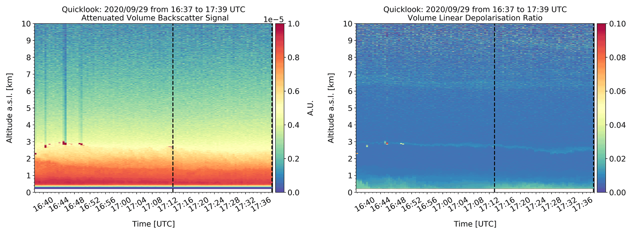
Figure 8Height versus time plots of the attenuated volume backscatter signal from linear emission and the volume linear depolarisation ratio at 355 nm over Athens, measured by eVe lidar on 29 September 2020 from 16:37 to 17:39 UTC. The raw temporal and vertical resolution are 30 s and 3.75 m, respectively, with vertical pointing of the system. The attenuated volume backscatter signal was calibrated using a calibration factor averaged inside the selected time frame and calculated at 3.8 km with a 0.3 km window. The two dashed black lines enclose the selected time frame for the optical products' retrieval.
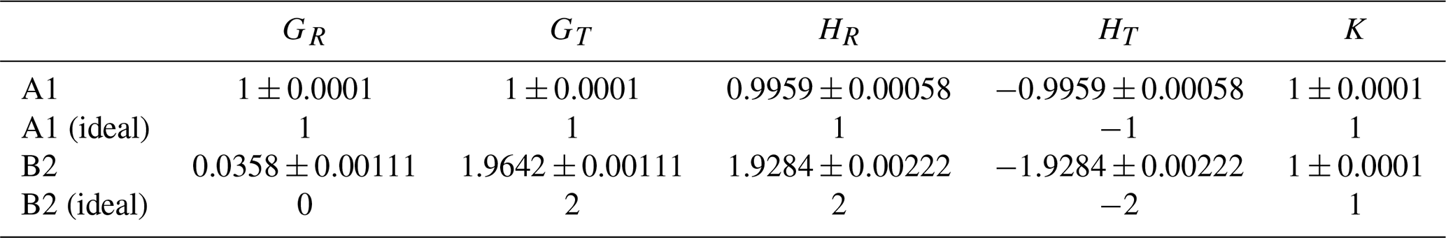
In the retrieval of the averaged profiles of volume linear and circular depolarisation ratios, the G, H, and K parameters that are applied in each lidar configuration (A1, B2) were used to correct the corresponding lidar signals from the polarisation crosstalk effects (see Sect. 4.2.3). Table 2 provides the G, H, and K parameters with the corresponding uncertainties that were used for the retrieval of the VLDR and VCDR profiles on 24 September 2020 and the theoretical (ideal) G, H, and K values according to Freudenthaler (2016).
Table 2The G, H, and K parameters with their uncertainties that were used for the retrieval of the VLDR and VCDR profiles on 29 September 2020 from the A1 and B2 lidar configurations, respectively. The ideal G, H, and K values for each configuration are also provided (Freudenthaler, 2016).

Figure 9 shows the optical products retrieved from the signals averaged over the selected time frame. The atmospheric volume over the site has low VLDR values since no values larger than the 0.016±0.0001 and 0.008±0.0002 are observed below 1.2 km and at approximately 2.6 km, respectively. The VCDR profile as well as the converted volume circular depolarisation ratio profile (VLDR-to-VCDR) are also shown in Fig. 9, where both the VCDR and VLDR-to-VCDR show values up to 0.032±0.0009 below 1.2 km and up to 0.016±0.0009 at approximately 2.6 km. The converted VLDR-to-VCDR is identical to the retrieved VCDR, confirming the theoretical relationship between linear and circular depolarisation ratio, since the calculated difference between the converted (VLDR-to-VCDR) and retrieved (VCDR) circular depolarisation ratios using the VCDR as reference is less than 0.0013. The corresponding PLDR values are in the order of 0.062±0.003 below 1.2 km and in the order of 0.03±0.011 at 2.6 km, indicating the presence of slightly depolarising particles at 2.6 km, while the PCDR values in the same altitude ranges are in the order of 0.1362±0.009 and 0.0778±0.0331, respectively. In all altitude ranges the differences between the PCDR and the converted PLDR-to-PCDR using the PCDR as reference are less than 0.037 and inside the statistical uncertainty of the retrieval.
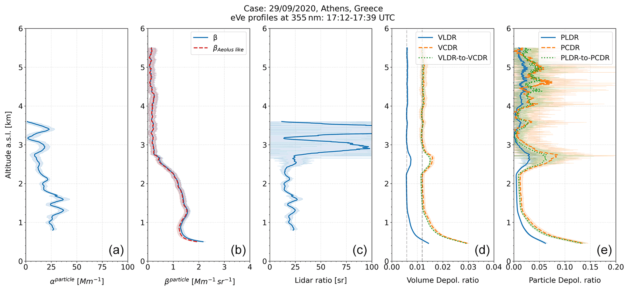
Figure 9Profiles of the particle extinction coefficient, the particle backscatter coefficient, the lidar ratio, the volume depolarisation ratios and the particle depolarisation ratios (from left to right) at 355 nm for the time frame 17:12 to 17:39 UTC on 29 September 2020. The Aeolus-like particle backscatter coefficient (βAeolus-like; dashed red line) and the particle backscatter coefficient (β; solid blue line) were both retrieved from the circularly polarised signals of eVe lidar using the Raman inversion method, where the reference height for Rayleigh atmosphere was selected at 10.3 km with a 0.3 km window. The VLDR and PLDR profiles are presented by solid blue lines, and the VCDR and PCDR profiles are presented by dashed orange lines, while the VLDR-to-VCDR and PLDR-to-PCDR profiles are presented by dotted green lines. The corresponding mLDR and mCDR values (dashed grey lines) that are expected to be measured by the lidar are also provided in the volume depolarisation ratio subplot. Shaded regions denote statistical 1σ uncertainty.
According to the profiles of the particle backscatter coefficient and the particle extinction coefficient in Fig. 9, the suspended particles form a thin layer that extends up to 2.6 km with backscatter coefficient values up to 2±0.1 Mm−1 sr−1. The extinction coefficient mean value up to 2.6 km is 22.7±4.29 Mm−1, and the corresponding mean lidar ratio value is 20±4.46 sr. Below 0.9 km the extinction coefficient and lidar ratio profiles are not available; thus only the backscatter coefficient and particle linear depolarisation ratio (PLDR ∼ 0.06) can be considered to characterise the suspended particles as a mixture of pollution and marine aerosols, according to Gross et al. (2015) and Illingworth et al. (2015). Above 0.9 km, the mean lidar ratio value is 20 sr, and the PLDR is below 0.03, indicating the presence of marine aerosols that may be mixed with traces of transported desert dust particles, even though the relative humidity (RH) values of less than 50 % in these heights could lead to crystallisation of the marine aerosols and higher PLDR values (Haarig et al., 2017). The RH profile was acquired from the nearest meteorological radiosonde (launched in Athens at 12:00 UTC) that was used for the optical products' retrieval, but it is not shown here.
Due to the absence of strongly depolarising particles in the atmospheric scene, a very good agreement in all altitude ranges with discrepancies less than 0.12 Mm−1 sr−1, which are inside the statistical uncertainty of the retrieval, can be observed between the profiles of the Aeolus-like backscatter coefficient and the backscatter coefficient in Fig. 9, denoting the expected good performance of Aeolus L2A products under scenes with negligible or no depolarisation.
5.2 Case study of 24 September 2020
On 24 September 2020, from 17:39 to 18:29 UTC, a layer with depolarising particles is present at approximately 4 km over Athens, as shown in the attenuated volume backscatter signal and VLDR profiles in Fig. 10. The depolarising particles may be transported desert dust particles according to the dust transport forecasting model BSC-DREAM8b records (https://dust.aemet.es/, last access: 3 March 2022) since the dust concentration at surface level was approximately 41 µg m−3. Above this layer, an aerosol-free region is observed up to 7 km. Depolarising layers are also detected between 7 and 8 km, which are not investigated further. From 18:02 to 18:25 UTC, a minor depolarising layer was present at 3 km, just below the mid-altitude layer. To avoid the retrieved optical products to be affected from this minor layer at 3 km and also aiming for homogeneous atmospheric conditions, the time frame between 17:39 and 18:02 UTC (enclosed by the dashed black lines in Fig. 10) was selected for the retrieval.
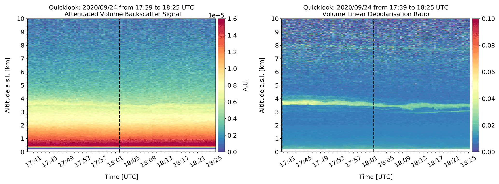
Figure 10Height versus time plots of the attenuated volume backscatter signal from linear emission and the volume linear depolarisation ratio at 355 nm over Athens, measured by eVe lidar on 24 September 2020 from 17:39 to 18:25 UTC. The raw temporal and vertical resolution is 30 s and 3.75 m, respectively, with vertical pointing of the system. The attenuated volume backscatter signal was calibrated using a calibration factor averaged inside the selected time frame and calculated at 9.8 km within a 0.2 km window. The two dashed black lines enclose the selected time frame for the optical products' retrieval.
Table 3 provides the G, H, and K parameters and their uncertainties that were used for the retrieval of the VLDR and VCDR profiles on 29 September 2020, and the theoretical (ideal) G, H, and K values according to Freudenthaler (2016). The values used for the G, H, and K parameters on 29 September 2020 approach the ideal G, H, and K values even better compared to the G, H, and K values used in the case of 24 September (Table 2). The main aim of the measurement period of September 2020 was the system optimisation using on-the-field measurements. Thus, the explanation of the improved G, H, and K values lies in the fine-tuning and readjustment of the HWP and QWPE angles, resulting in the reduction of the polarisation crosstalk effects introduced in the system by the misalignment of these optical elements.
Table 3The G, H, and K parameters with their uncertainties that were used for the retrieval of the VLDR and VCDR profiles on 24 September 2020. The ideal G, H, and K values for each configuration are also provided (Freudenthaler, 2016).
The retrievals inside the selected time frame of the volume and particle depolarisation ratios are shown in Fig. 11, where the depolarising layer extends from 3.4 to 3.9 km with mean VLDR and VCDR values of 0.0314±0.0006 and 0.07±0.0020, respectively, and PLDR and PCDR values up to 0.0893±0.007 and 0.213±0.017, respectively, indicating a layer with moderately depolarising particles. An optically thinner layer, with mean VLDR and VCDR values of 0.011±0.0003 and 0.020±0.0013, respectively, and mean PLDR and PCDR values of 0.028±0.002 and 0.05±0.0073, respectively, is observed in the lower altitude ranges, which gradually decreases with increasing altitude. At approximately 5.3 km an optically thinner layer is observed as well, with mean VLDR and VCDR values of 0.007±0.0006 and 0.014±0.002, respectively. The corresponding PLDR and PCDR values are in the order of 0.041±0.026 and 0.094±0.067, respectively.
In the depolarising layer within the height range between 3.4 and 3.9 km, where the aerosol load increases, a deviation of 0.005 is observed between the retrieved VCDR and the converted VLDR-to-VCDR. The same applies also for the particle circular depolarisation ratio, where a deviation of 0.019 is observed between the retrieved PCDR and the converted PLDR-to-PCDR. These differences indicate deviation of the measurements from the theoretical relationship that connects the linear and circular depolarisation ratio. This deviation can arise when the particles are oriented and/or when multiple scattering is significant. However, this assumption should be further investigated using more measurements over a wide variety of aerosol types and loads in the atmosphere. In addition, the converted PLDR-to-PCDR deviates from the retrieved PCDR by 0.02 above 5 km where the statistical uncertainty of retrieval in these altitude ranges (Fig. 11) is as high as 0.12.
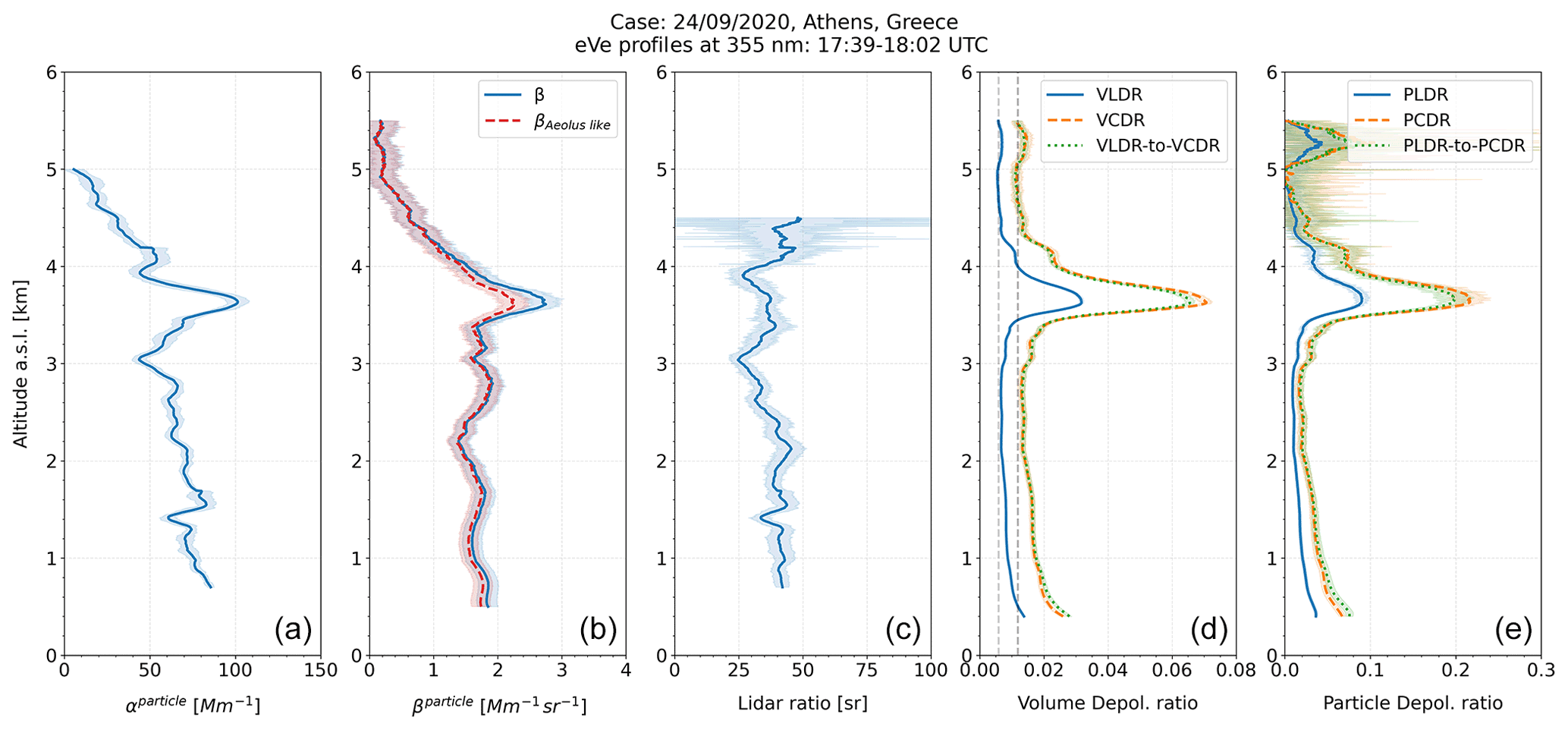
Figure 11Profiles of the particle extinction coefficient, the particle backscatter coefficient, the lidar ratio, the volume depolarisation ratios and the particle depolarisation ratios (from left to right) at 355 nm for the time frame 17:39 to 18:02 UTC on 24 September 2020. The Aeolus-like particle backscatter coefficient (βAeolus-like; dashed red line) and the particle backscatter coefficient (β; solid blue line) were both retrieved from the circularly polarised signals of eVe lidar using the Raman inversion method where the reference height for Rayleigh atmosphere was selected at 9.8 km within a 0.2 km window. The VLDR and PLDR profiles are presented by solid blue lines, the VCDR and PCDR profiles are presented by dashed orange lines, while the VLDR-to-VCDR and PLDR-to-PCDR profiles are presented by dotted green lines. The corresponding mLDR and mCDR values (dashed grey lines) that are expected to be measured by the lidar are also provided in the volume depolarisation ratio subplot. Shaded regions denote statistical 1σ uncertainty.
For this case, the particles inside the depolarising layer located from 3.4 to 3.9 km have backscatter values in the order of 2.69±0.22 Mm−1 sr−1, mean particle extinction coefficient of 99.7±7.18 Mm−1 (Fig. 11), and mean lidar ratio value of 37±4.56 sr. Below the base of the depolarising layer at 3.4 km, aerosols are also suspended in the atmosphere since the backscatter values range from 1.4 to 1.9 Mm−1 sr−1, and the extinction values range from 44 to 85 Mm−1. Moreover, the Aeolus-like backscatter coefficient in Fig. 11 is slightly underestimated by approximately 18 % with respect to the backscatter coefficient under the presence of the depolarising particles inside the detected layer at about 3.7 km. An even slighter underestimation of the Aeolus-like backscatter coefficient, in the order of 6 %, is detected below 2 km, but the corresponding deviations fall within the calculated statistical uncertainty of the retrieval.
The eVe lidar is a combined linear–circular polarisation system with Raman capabilities operating at 355 nm. The lidar is specially designed to provide ground-based reference measurements for Cal/Val studies on Aeolus L2A products. The system is also ideal for future EarthCARE Cal/Val activities, due to its linear polarisation measurements and its mobility that allows for positioning on the satellite track, a condition that is mandatory for the Cal/Val of spaceborne lidars due to their small footprint. In this paper we described the hardware of the system and the outcome of the applied polarisation calibration techniques, as well as the developed algorithm for retrieving the optical products of eVe, along with two selected cases among the first conducted measurements in Athens. The applied techniques for calculating the polarisation calibration factor and diagnosing unwanted polarising effects in system will be discussed in detail in a future study. In the first case we examined slightly depolarising particles that are present in the atmosphere at approximately 2.6 km, with VLDR and VCDR values of 0.008±0.0002 and 0.016±0.0009, respectively, and corresponding PLDR and PCDR values of 0.03±0.011 and 0.0778±0.0331. In addition, the converted VLDR-to-VCDR and the PLDR-to-PCDR profiles present a very good agreement with respect to the retrieved VCDR and PCDR profiles, respectively. The same applies also between the profiles of the particle backscatter coefficient and the Aeolus-like backscatter coefficient, as expected in such atmospheric conditions. In the second case, the suspended particles in the layer extending from 3.4 to 3.9 km are moderately depolarising with VLDR and VCDR values of 0.0314±0.0006 and 0.07±0.0020, respectively, and corresponding PLDR and PCDR values of 0.0893±0.007 and 0.213±0.017, respectively. Inside the depolarising layer where the AOD is increased with respect to the rest profile, the converted volume and particle circular depolarisation ratios (VLDR-to-VCDR and PLDR-to-PCDR) deviate from the retrieved ones (VCDR and PCDR) by 0.005 and 0.019, respectively, falling within the related statistical uncertainties. In addition, an underestimation of 18 % is observed for the Aeolus-like backscatter coefficient with respect to the measured particle backscatter coefficient.
Besides eVe's main goal of providing reference measurements for Cal/Val studies on ESA's satellite missions, an interesting application of eVe lidar is related to the possible differences between circular and linear polarisation, caused most probably by multiple scattering and particle orientation effects. This effect could possibly increase due to the AOD and for non-spherical particles (Mishchenko and Hovenier, 1995; Roy and Roy, 2008), as is slightly indicated by the two case studies presented in this work. Multiple scattering effects in dust layers have only been detected from instruments on board satellite platforms like CALIPSO (Wandinger et al., 2010; Yoshida et al., 2010). On the other hand, regarding the randomly oriented particles' assumption, it has recently been reported theoretically in Mallios et al. (2021) and experimentally in Daskalopoulou et al. (2021) that the dust particles can have a preferential vertical plane of orientation. Thus, the particle orientation seems to be a reasonable explanation for the observed deviations between the converted and retrieved circular depolarisation ratios in case of desert dust. Nevertheless, the validity of the theoretical relationship between linear and circular depolarisation ratio has to be further investigated by performing more measurements in dust layers, cirrus clouds, and/or scenes when different aerosol types are probed, before a definite explanation is given. An added value in this kind of study will be the collocated measurements with the polarisation lidar of the National Observatory of Athens (NOA), nicknamed “WALL-E” (Tsekeri et al., 2021), which is specifically designed to detect and characterise dust particle orientation. In addition, the concept of a dual-FOV technique (Jimenez et al., 2020b) can be implemented in the system in order to attempt to extract information about the multiple scattering contribution on dust layers. These aspects will be examined in the future using eVe measurements that are collected during the experimental campaigns that have been scheduled by ESA, for example, the ASKOS experiment under the Joint Aeolus Tropical Atlantic Campaign 2021 (JATAC) on the islands of Cabo Verde.
A1 Theoretical background
The laser beam emitted from a lidar system interacts with the atmospheric constituents, and part of it is scattered at the backward direction. The total backscattered light is quantified using the backscatter coefficient (β), defined in cloud-free atmospheres as the sum of the particle (i.e. aerosol) backscatter coefficient (βp) and the molecular backscatter coefficient (βm).
The lidar ratio (L) is defined as the ratio of the extinction to backscatter coefficients. The particle backscatter-to-extinction ratio (BER) is the inverted particle lidar ratio Lp.
In a lidar setup the measured total signal from the collected backscattered light is described by the following equation:
where A0 is the system constant, C is the calibration factor, and T2(z) is the atmospheric transmittance from the lidar to the scattering volume and back.
In polarisation-sensitive lidar systems the backscattered light from linearly or circularly polarised emission is optically separated with a polarisation analyser in two components, and thus two signals can be measured. The parallel or co-polar component (∥) contains the backscattered light with the original polarisation and half of the depolarised light, whereas the cross or cross-polar component (⊥) contains the other half of the depolarised light (Gimmestad, 2008). According to Gimmestad (2008), in case of randomly oriented particles in the atmosphere and for single-scattered light backwards, the lidar equations of the two measured signal components can be written as
and
In the lidar, Eqs. (A4) and (A5) of the measured signals depend on the atmospheric polarisation parameter a (Freudenthaler, 2016), that is the atmospheric depolarisation parameter d of Gimmestad (2008). The atmospheric polarisation parameter a, together with the backscatter coefficient β, fully characterises an atmospheric scattering volume, consisting of arbitrary-shaped particles and their mirror particles in random orientation (Mishchenko and Hovenier, 1995). Due to the fact that the direction of light propagation from backscattering is reversed, and the reference coordination system for defining the polarisation state is changed accordingly, the handedness of the backscattered circularly polarised light is inverted (Freudenthaler, 2016, Sect. 6; Gimmestad, 2008). The functions f∥ and f⊥ describe the result of the interaction of the emitted polarised light with the atmosphere and the optical elements of the lidar. For linearly polarised emission and a linear polarisation analyser in the lidar receiver, the functions in the measured signal components are
while, for the circularly polarised emission and circular polarisation analyser in the lidar setup, the functions are
The total backscatter coefficient for different scatterer types i (p for particles, m for molecules, and v for volume) and for emitted light of linear or circular polarisation ( can be written as
Mishchenko and Hovenier (1995) define the depolarisation ratio (δ) as the ratio of the cross or cross-polar to the parallel or co-polar measured signal components depending on the polarisation state of the emission (linear or circular). The signal ratio is corrected with the polarisation calibration factor (, which includes their relative amplification differences (Freudenthaler, 2016). Hence, the depolarisation ratio that holds for linear and circular polarisation can be derived using the polarisation parameter a.
Depending on the scatterer type i (, the linear depolarisation ratio ( is obtained from Eq. (A12), while the circular depolarisation ratio ( is obtained from Eq. (A13).
Equation (A14) is derived using Eqs. (A12) and (A13) and provides the relation between the linear depolarisation ratio ( and the circular depolarisation ratio (, in case of randomly oriented particles in the atmosphere and under a single-scattering assumption (Mishchenko and Hovenier, 1995; Roy and Roy, 2008):
On the contrary, under the presence of oriented particles and/or multiple scattering conditions, the off-diagonal elements of the backscatter Müller matrix F of the atmosphere may be non-zero, and the same can also be true for the scattering Müller matrices that model the other scattering processes at different angles than 180∘ (van de Hulst, 1957; Mishchenko and Hovenier, 1995). Under these conditions the interaction of polarised light with the atmosphere will be not described by Eqs. (A6) to (A9), and the theoretical relationship between the linear and circular depolarisation ratio (Eq. A14) does not hold.
A2 How to convert the polarisation lidar products to Aeolus L2A optical products
Since ALADIN on board Aeolus only detects the co-polar component of the backscattered circularly polarised light, the lidar equation that describes the detected signal is Eq. (A4). Consequently, Aeolus retrieves the quantity named as the co-polar backscatter coefficient. The co-polar backscatter coefficient does not have a physical meaning (Gimmestad, 2008), and it is used only to name the quantity that is retrieved from Aeolus as the L2A product of the particle backscatter coefficient.
The ground-based polarisation lidars can use their measurements of the particle backscatter coefficient, the lidar ratio, and the volume and particle depolarisation ratios to derive products that are comparable with the Aeolus L2A products with the following steps:
-
The particle linear depolarisation ratio ( retrieved from ground-based polarisation lidar with linearly polarised emission can be converted to the particle circular depolarisation ratio ( using Eq. (A14).
-
The particle backscatter coefficient (βp) is converted to the Aeolus-like backscatter coefficient (βAeolus-like) using Eqs. (A10) and (A11):
-
The Aeolus-like particle BER is calculated using the Aeolus-like backscatter coefficient from Eq. (A15):
Thus, the Aeolus-like lidar ratio (LAeolus-like) is derived using Lp and :
Several quality assurance tools, such as the Rayleigh fit, the telecover test, the polarisation calibration, and the dark measurement, are being applied throughout the lidar systems in the EARLINET network (Freudenthaler et al., 2018; Pappalardo et al., 2014), aiming to harmonise the measurements from the different operating lidar systems throughout the network, to monitor the quality of the lidar measurements, to identify changes or degradation issues in the lidar's hardware, and to improve the lidar performance and the quality of the measurements. Although eVe lidar is not part of the EARLINET network, the network's quality assurance tools are also being applied in the eVe lidar in order to test the good performance of the lidar. In this Appendix, the results from a telecover test and a Rayleigh fit test that were performed on eVe lidar are presented.
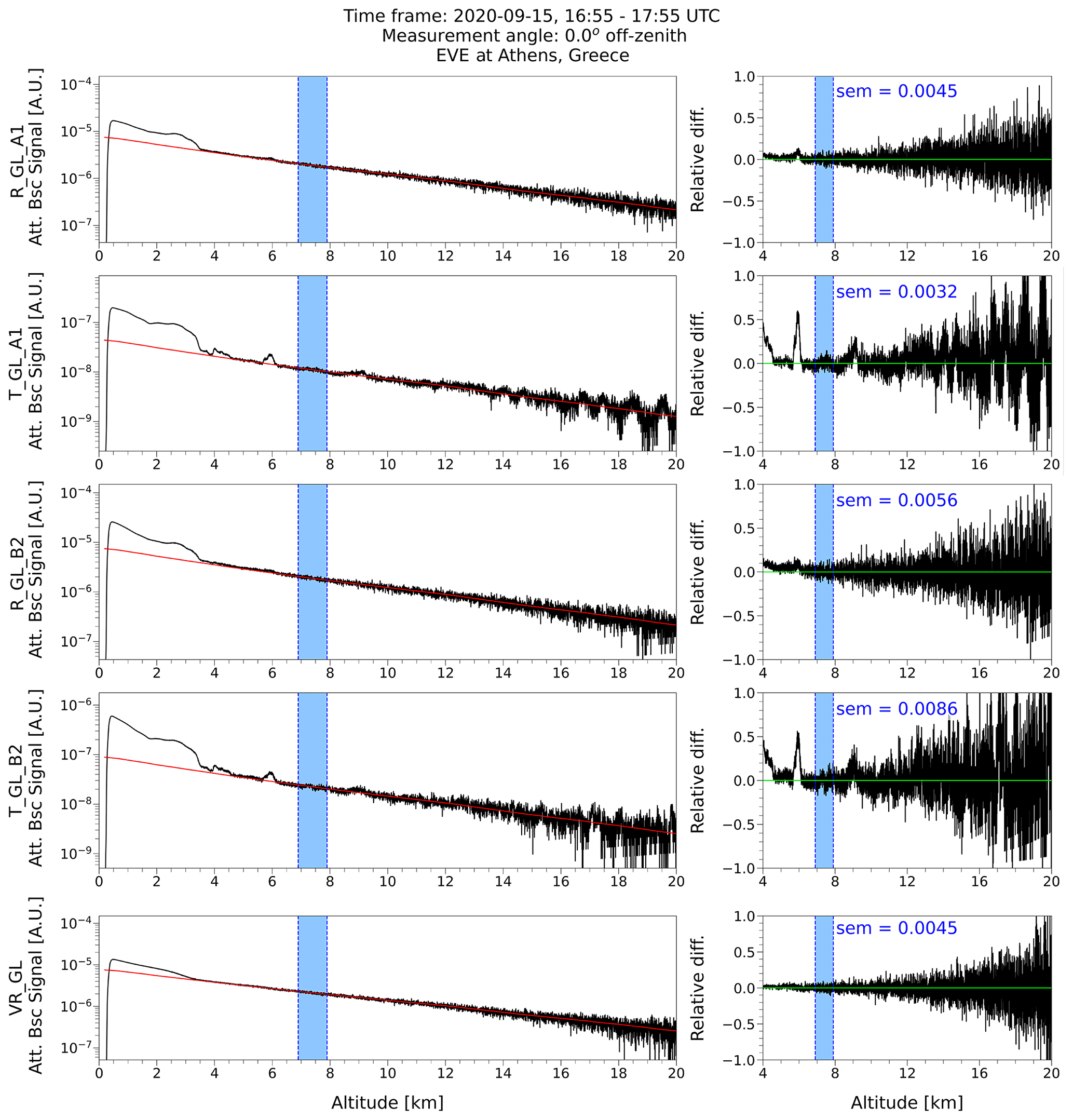
Figure B1The Rayleigh fit test from a 1 h night-time measurement with vertical pointing of the lidar on 15 September 2020. In the first column, the elastic unsmoothed range-corrected glued signals from the reflected (R_GL) and transmitted (T_GL) channels of the A1 and B2 configurations and the inelastic unsmoothed range-corrected glued signal from the Raman channel (VR_GL) are normalised to the corresponding Rayleigh signals (red line) over the shaded blue region. In the second column, the relative difference of the normalised signals from the Rayleigh signals is presented, along with the standard error of the mean (SEM) of the differences inside the reference region. The blue shaded region denotes the selected reference region for Rayleigh atmosphere (7.4±0.5 km).
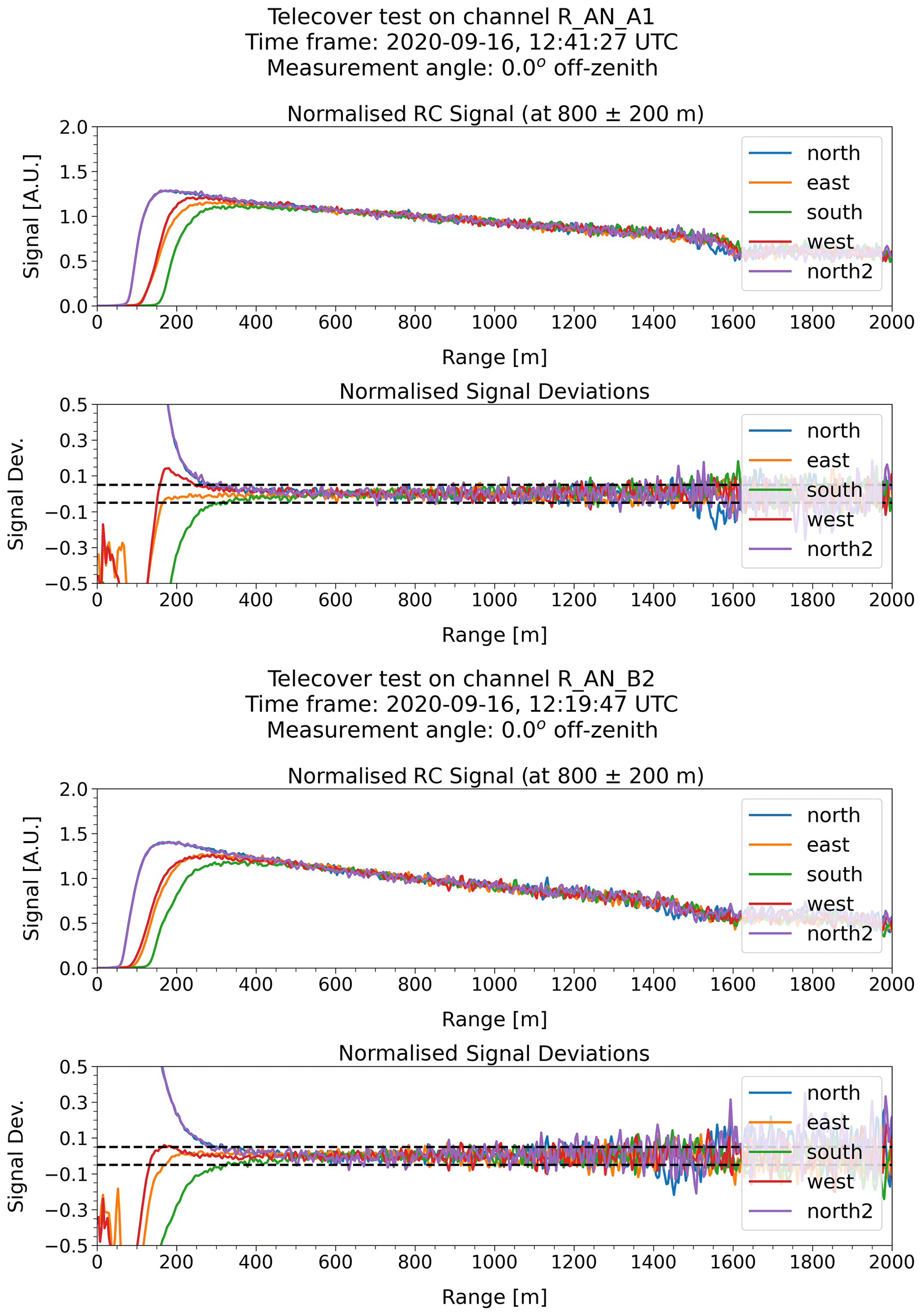
Figure B2The octant telecover test using the telecover signals from the Reflected (R) channels of the A1 and B2 configurations on 16 September 2020. The signals are unsmoothed range-corrected analogue signals normalised at 800 m with a window of 400 m where the north (blue), east (orange), west (red), south (green), north2 (purple) indicate the measured telecover sector. The provided signal deviation is the relative deviation of the normalised signal from the mean.
The Rayleigh fit test in Fig. B1 was performed on 15 September 2020 during a 1 h night-time measurement and shows the normalised elastic signals detected in the R and T channels of A1 and B2 configurations and the normalised inelastic signal detected in the Raman channel compared with the corresponding Rayleigh signals (i.e. the calculated attenuated molecular backscatter coefficient). The lidar signals that are shown are detected from the operational lidar configurations (A1, B2) that are used for the optical products' retrieval. The lidar signals are normalised to the corresponding Rayleigh signals in a selected Rayleigh region indicated by the reference height (Freudenthaler et al., 2018). Additionally, the relative difference of the normalised lidar signals from the corresponding Rayleigh signals calculated in each height bin, as well as the standard error of the mean (SEM) of the differences calculated inside the reference region, are shown in the right column of Fig. B1. By inspecting the Rayleigh fit test of the cross-polarised signals from linear and circular emission (detected in the R channel of A1 and B2 configurations, respectively) and their corresponding relative differences from the Rayleigh signals, the reference height was selected at 7.4 km with an averaging window of 1 km. Inside the selected region, the cross-polarised signals are well fitted with the Rayleigh signals, and the SEM of the difference is below 0.0086 for all signals. Below the height of 9.8 km the elastic signals deviate from the corresponding Rayleigh signals with relative differences above 10 %, indicating the presence of aerosols.
A Rayleigh fit test was also performed during the selected cases (24 and 29 September 2020) for the determination of the reference height, but it is not shown here. For both of the measurement cases, the Rayleigh fit test was used for the determination of the reference height region for the Rayleigh atmosphere because the reference height is required as an input in the retrieval of the particle backscatter coefficient.
Furthermore, the Rayleigh fit test can provide indication of misalignment of the system in the far-range region when the normalised lidar signals deviate abnormally from the Rayleigh signals in the far range (e.g. negative deviation of the normalised signal from the Rayleigh signal), as long as these deviations cannot be attributed to normalisation of the lidar signals inside a non-Rayleigh region, to the presence of aerosols or clouds, or to signal distortions (for analogue signals). In the case of 15 September 2020 (Fig. B1) the normalised lidar signals fit well with the Rayleigh signals in the Rayleigh region (above 9 km), indicating the good system alignment in the far range. In order to examine whether the system alignment is good also in the near range and to determine the distance of full overlap, a telecover test has to be performed (Freudenthaler et al., 2018). The nearest telecover test from 15 September is the one performed on 16 September 2020 (Fig. B2) when the lidar had the same pointing angle, and no change of the pointing geometry was made in between.
The telecover test was performed during the daytime using the analogue signals instead of the photon-counting signals since the analogue signals are optimised for the near range, while the photon-counting signals are optimised for the far range. The normalised signals from the octant telecover test (i.e. using the outer parts of the quadrants) show that for both A1 and B2 configurations, the laser beam inserts the telescope's FOV firstly and mostly from the north sector, which is closer to the laser beam based on the laser–telescope geometry (diamond-shaped), followed by the east and west sectors, which are equally distanced from the beam, and finally by the south sector, which is the farthest sector from the beam. The relative deviations from the mean for all sectors are the largest in the first metres where the laser beam has not yet fully entered into the telescope's FOV, and they start to decrease with range and as the laser beam enters the FOV. The full overlap of the system is reached at 400 m, taking into account a threshold value of 5 % in the relative deviations from the mean (Freudenthaler et al., 2018).
The software code used in this work is available upon request.
The data that are presented in this work are publicly available in the Zenodo public data repository at https://doi.org/10.5281/zenodo.6359726 (Paschou et al., 2022).
PP and NS tested and optimised the instrument and acquired the measurements shown herein with the support of AL, GG, AT, GT, CE, and VF. PP and NS developed the software for processing the measurements and performing quality assurance tests and retrieving the optical products. NS and VF formulated the measurement strategy and the emission and detection design of the system, along with the calibration procedures. VF conceived the “dual-laser/dual-telescope” concept, and GG and AL developed the optomechanical design of the instrument. VF provided the temperature dependent molecular linear depolarisation ratio profiles based on the lidar's interference filters specs. PP did the analysis of the acquired measurements and the manuscript preparation with the support of NS. VF, AT, VA, IB, and JvB provided corrections and suggestions. VA supervised and directed the whole project. All authors provided critical feedback and helped shape the research, analysis, and manuscript.
At least one of the (co-)authors is a member of the editorial board of Atmospheric Measurement Techniques. The peer-review process was guided by an independent editor. Alexandros Louridas, George Georgoussis, Ioannis Binietoglou, George Tsaknakis, Alexandros Tavernarakis, and Christos Evangelatos are employed at Raymetrics S.A. and were involved in the development and manufacturing of the lidar system.
Publisher's note: Copernicus Publications remains neutral with regard to jurisdictional claims in published maps and institutional affiliations.
This article is part of the special issue “Aeolus data and their application (AMT/ACP/WCD inter-journal SI)”. It is not associated with a conference.
The authors acknowledge the support of the Stavros Niarchos Foundation and the support of Giuseppe D’Amico in the calculation of the temperature-dependent molecular linear depolarisation ratio profiles based on the lidar's interference filters' specifications. The lidar system was developed under an European Space Agency project by Raymetrics S.A. in collaboration with the National Observatory of Athens and the Ludwig-Maximilians-Universität.
This research has been supported by the “PANhellenic infrastructure for Atmospheric Composition and climatE change” (MIS 5021516), implemented under the Action “Reinforcement of the Research and Innovation Infrastructure”, funded by the Operational Programme “Competitiveness, Entrepreneurship and Innovation” (NSRF 2014-2020) and co-financed by Greece and the European Union (European Regional Development Fund); the European Research Council under the European Community's Horizon 2020 Research and Innovation framework programme/ERC D-TECT (grand no. 725698); and the European Space Agency (grant no. 4000127438/19/I-BG).
This paper was edited by Oliver Reitebuch and reviewed by Ronny Engelmann and one anonymous referee.
Ansmann, A., Wandinger, U., Riebesell, M., Weitkamp, C., and Michaelis, W.: Independent measurement of extinction and backscatter profiles in cirrus clouds by using a combined Raman elastic-backscatter lidar, Appl. Opt., 31, 7113–7131, https://doi.org/10.1364/AO.31.007113, 1992.
Ansmann, A., Wandinger, U., Le Rille, O., Lajas, D., and Straume, A. G.: Particle backscatter and extinction profiling with the spaceborne high-spectral-resolution Doppler lidar ALADIN: methodology and simulations, Appl. Opt., 46, 6606, https://doi.org/10.1364/AO.46.006606, 2007.
Ansmann, A., Tesche, M., Groß, S., Freudenthaler, V., Seifert, P., Hiebsch, A., Schmidt, J., Wandinger, U., Mattis, I., Müller, D., and Wiegner, M.: The 16 April 2010 major volcanic ash plume over central Europe: EARLINET lidar and AERONET photometer observations at Leipzig and Munich, Germany, Geophys. Res. Lett., 37, L13810, https://doi.org/10.1029/2010GL043809, 2010.
Baars, H., Kanitz, T., Engelmann, R., Althausen, D., Heese, B., Komppula, M., Preißler, J., Tesche, M., Ansmann, A., Wandinger, U., Lim, J.-H., Ahn, J. Y., Stachlewska, I. S., Amiridis, V., Marinou, E., Seifert, P., Hofer, J., Skupin, A., Schneider, F., Bohlmann, S., Foth, A., Bley, S., Pfüller, A., Giannakaki, E., Lihavainen, H., Viisanen, Y., Hooda, R. K., Pereira, S. N., Bortoli, D., Wagner, F., Mattis, I., Janicka, L., Markowicz, K. M., Achtert, P., Artaxo, P., Pauliquevis, T., Souza, R. A. F., Sharma, V. P., van Zyl, P. G., Beukes, J. P., Sun, J., Rohwer, E. G., Deng, R., Mamouri, R.-E., and Zamorano, F.: An overview of the first decade of PollyNET: an emerging network of automated Raman-polarization lidars for continuous aerosol profiling, Atmos. Chem. Phys., 16, 5111–5137, https://doi.org/10.5194/acp-16-5111-2016, 2016.
Behrendt, A., Pal, S., Wulfmeyer, V., Valdebenito B., Á. M., and Lammel, G.: A novel approach for the characterization of transport and optical properties of aerosol particles near sources – Part I: Measurement of particle backscatter coefficient maps with a scanning UV lidar, Atmos. Environ., 45, 2795–2802, https://doi.org/10.1016/j.atmosenv.2011.02.061, 2011.
Belegante, L., Bravo-Aranda, J. A., Freudenthaler, V., Nicolae, D., Nemuc, A., Ene, D., Alados-Arboledas, L., Amodeo, A., Pappalardo, G., D'Amico, G., Amato, F., Engelmann, R., Baars, H., Wandinger, U., Papayannis, A., Kokkalis, P., and Pereira, S. N.: Experimental techniques for the calibration of lidar depolarization channels in EARLINET, Atmos. Meas. Tech., 11, 1119–1141, https://doi.org/10.5194/amt-11-1119-2018, 2018.
Beyerle, G.: Untersuchungen stratosphärischer Aerosole vulkanischen Ursprungs und polarer stratosphärischer Wolken mit einem Mehrwellen-Lidar auf Spitzbergen (79∘ N, 12∘ E) = Multiwavelength lidar measurements of stratospheric volcanic aerosols and polar stratospheric c, Berichte zur Polarforsch. (Reports Polar Res., 138, https://doi.org/10.2312/BzP_0138_1994, 1994.
Böckmann, C., Wandinger, U., Ansmann, A., Bösenberg, J., Amiridis, V., Boselli, A., Delaval, A., Tomasi, F. De, Frioud, M., Grigorov, I. V., Hågård, A., Horvat, M., Iarlori, M., Komguem, L., Kreipl, S., Larchevêque, G., Matthias, V., Papayannis, A., Pappalardo, G., Rocadenbosch, F., Rodrigues, J. A., Schneider, J., Shcherbakov, V., and Wiegner, M.: Aerosol lidar intercomparison in the framework of the EARLINET project. 2.Aerosol backscatter algorithms, Appl. Opt., 43, 977–989, https://doi.org/10.1364/AO.43.000977, 2004.
Chipman, R. A.: Mueller matrices, in Handbook of Optics: Volume I – Geometrical and Physical Optics, Polarized Light, Components and Instruments, 3rd Edition, edited by: Bass, M., McGraw-Hill Professional, USA, 1248 pp., 2009a.
Chipman, R. A.: Polarimetry, in: Handbook of Optics: Volume I – Geometrical and Physical Optics, Polarized Light, Components and Instruments, 3rd Edition, edited by: Bass, M., McGraw-Hill Professional, USA, 1248 pp., 2009b.
D'Amico, G., Amodeo, A., Mattis, I., Freudenthaler, V., and Pappalardo, G.: EARLINET Single Calculus Chain – technical – Part 1: Pre-processing of raw lidar data, Atmos. Meas. Tech., 9, 491–507, https://doi.org/10.5194/amt-9-491-2016, 2016.
Dabas, A.: Observing the atmospheric wind from space, C. R. Geosci., 342, 370–379, https://doi.org/10.1016/J.CRTE.2009.09.014, 2010.
Daskalopoulou, V., Raptis, I. P., Tsekeri, A., Amiridis, V., Kazadzis, S., Ulanowski, Z., Metallinos, S., Tassis, K., and Martin, W.: Monitoring dust particle orientation with measurements of sunlight dichroic extinction, 15th International Conference on Meteorology, Climatology and Atmospheric Physics (COMECAP 2021), Ioannina, Greece, 26–29 September 2021, Zenodo [conference paper], https://doi.org/10.5281/zenodo.5075998, 2021.
Donovan, D. P., Whiteway, J. A., and Carswell, A. I.: Correction for nonlinear photon-counting effects in lidar systems, Appl. Opt., 32, 6742, https://doi.org/10.1364/AO.32.006742, 1993.
Donovan, D. P., Klein Baltink, H., Henzing, J. S., de Roode, S. R., and Siebesma, A. P.: A depolarisation lidar-based method for the determination of liquid-cloud microphysical properties, Atmos. Meas. Tech., 8, 237–266, https://doi.org/10.5194/amt-8-237-2015, 2015.
Engelmann, R., Kanitz, T., Baars, H., Heese, B., Althausen, D., Skupin, A., Wandinger, U., Komppula, M., Stachlewska, I. S., Amiridis, V., Marinou, E., Mattis, I., Linné, H., and Ansmann, A.: The automated multiwavelength Raman polarization and water-vapor lidar PollyXT: the neXT generation, Atmos. Meas. Tech., 9, 1767–1784, https://doi.org/10.5194/amt-9-1767-2016, 2016.
Evans, R. D.: The atomic nucleus, McGraw-Hill, New York, 992 pp., 1955.
Fernald, F. G.: Analysis of atmospheric lidar observations: some comments, Appl. Opt., 23, 652–653, https://doi.org/10.1364/AO.23.000652, 1984.
Flamant, P., Lever, V., Martinet, P., Flament, T., Cuesta, J., Dabas, A., M., O., and Huber, D.: AE-TN-IPSL-GS-001 v5.7: ADM-Aeolus L2A Algorithm Theoretical Baseline Document, https://earth.esa.int/eogateway/documents/20142/37627/Aeolus-L2A-Algorithm-Theoretical-Baseline-Document (last access: 30 August 2021), 2007.
Flamant, P., Cuesta, J., Denneulin, M.-L., Dabas, A., and Huber, D.: ADM-Aeolus retrieval algorithms for aerosol and cloud products, Tellus A, 60, 273–288, https://doi.org/10.1111/j.1600-0870.2007.00287.x, 2008.
Freudenthaler, V.: Effects of spatially inhomogeneous photomultiplier sensitivity on lidar signals and remedies, in: 22nd Internation Laser Radar Conference (ILRC 2004), Vol. 561, p. 37, 2004.
Freudenthaler, V.: About the effects of polarising optics on lidar signals and the Δ90 calibration, Atmos. Meas. Tech., 9, 4181–4255, https://doi.org/10.5194/amt-9-4181-2016, 2016.
Freudenthaler, V., Esselborn, M., Wiegner, M., Heese, B., Tesche, M., Ansmann, A., Müller, D., Althausen, D., Wirth, M., Fix, andreas, Ehret, G., Knippertz, P., Toledano, C., Gasteiger, J., Garhammer, M., and Seefeldner, M.: Depolarization ratio profiling at several wavelengths in pure Saharan dust during SAMUM 2006, Tellus B, 61, 165–179, https://doi.org/10.1111/j.1600-0889.2008.00396.x, 2009.
Freudenthaler, V., Linné, H., Chaikovski, A., Rabus, D., and Groß, S.: EARLINET lidar quality assurance tools, Atmos. Meas. Tech. Discuss. [preprint], https://doi.org/10.5194/amt-2017-395, in review, 2018.
Gialitaki, A., Tsekeri, A., Amiridis, V., Ceolato, R., Paulien, L., Kampouri, A., Gkikas, A., Solomos, S., Marinou, E., Haarig, M., Baars, H., Ansmann, A., Lapyonok, T., Lopatin, A., Dubovik, O., Groß, S., Wirth, M., Tsichla, M., Tsikoudi, I., and Balis, D.: Is the near-spherical shape the “new black” for smoke?, Atmos. Chem. Phys., 20, 14005–14021, https://doi.org/10.5194/acp-20-14005-2020, 2020.
Giannakaki, E., Pfüller, A., Korhonen, K., Mielonen, T., Laakso, L., Vakkari, V., Baars, H., Engelmann, R., Beukes, J. P., Van Zyl, P. G., Josipovic, M., Tiitta, P., Chiloane, K., Piketh, S., Lihavainen, H., Lehtinen, K. E. J., and Komppula, M.: One year of Raman lidar observations of free-tropospheric aerosol layers over South Africa, Atmos. Chem. Phys., 15, 5429–5442, https://doi.org/10.5194/acp-15-5429-2015, 2015.
Gimmestad, G. G.: Reexamination of depolarization in lidar measurements, Appl. Opt., 47, 3795, https://doi.org/10.1364/AO.47.003795, 2008.
Gross, S., Freudenthaler, V., Wirth, M., and Weinzierl, B.: Towards an aerosol classification scheme for future EarthCARE lidar observations and implications for research needs, Atmos. Sci. Lett., 16, 77–82, https://doi.org/10.1002/asl2.524, 2015.
Haarig, M., Ansmann, A., Gasteiger, J., Kandler, K., Althausen, D., Baars, H., Radenz, M., and Farrell, D. A.: Dry versus wet marine particle optical properties: RH dependence of depolarization ratio, backscatter, and extinction from multiwavelength lidar measurements during SALTRACE, Atmos. Chem. Phys., 17, 14199–14217, https://doi.org/10.5194/acp-17-14199-2017, 2017.
Holben, B. N., Eck, T. F., Slutsker, I., Tanré, D., Buis, J. P., Setzer, A., Vermote, E., Reagan, J. A., Kaufman, Y. J., Nakajima, T., Lavenu, F., Jankowiak, I., and Smirnov, A.: AERONET – A federated instrument network and data archive for aerosol characterization, Remote Sens. Environ., 66, 1–16, https://doi.org/10.1016/S0034-4257(98)00031-5, 1998.
van de Hulst, H. C.: Light scattering by small particles, Wiley, New York, 470 pp., 1957.
Illingworth, A. J., Barker, H. W., Beljaars, A., Ceccaldi, M., Chepfer, H., Clerbaux, N., Cole, J., Delanoë, J., Domenech, C., Donovan, D. P., Fukuda, S., Hirakata, M., Hogan, R. J., Huenerbein, A., Kollias, P., Kubota, T., Nakajima, T., Nakajima, T. Y., Nishizawa, T., Ohno, Y., Okamoto, H., Oki, R., Sato, K., Satoh, M., Shephard, M. W., Velázquez-Blázquez, A., Wandinger, U., Wehr, T., and Van Zadelhoff, G. J.: The earthcare satellite: The next step forward in global measurements of clouds, aerosols, precipitation, and radiation, B. Am. Meteorol. Soc., 96, 1311–1332, https://doi.org/10.1175/BAMS-D-12-00227.1, 2015.
Imaki, M., Takegoshi, Y., and Kobayashi, T.: Ultraviolet High-Spectral-Resolution Lidar with Fabry – Perot Filter for Accurate Measurement of Extinction and Lidar Ratio, Jpn. J. Appl. Phys., 44, 3063–3067, https://doi.org/10.1143/JJAP.44.3063, 2005.
Jimenez, C., Ansmann, A., Engelmann, R., Donovan, D., Malinka, A., Seifert, P., Wiesen, R., Radenz, M., Yin, Z., Bühl, J., Schmidt, J., Barja, B., and Wandinger, U.: The dual-field-of-view polarization lidar technique: a new concept in monitoring aerosol effects in liquid-water clouds – case studies, Atmos. Chem. Phys., 20, 15265–15284, https://doi.org/10.5194/acp-20-15265-2020, 2020a.
Jimenez, C., Ansmann, A., Engelmann, R., Donovan, D., Malinka, A., Schmidt, J., Seifert, P., and Wandinger, U.: The dual-field-of-view polarization lidar technique: a new concept in monitoring aerosol effects in liquid-water clouds – theoretical framework, Atmos. Chem. Phys., 20, 15247–15263, https://doi.org/10.5194/acp-20-15247-2020, 2020b.
Klett, J. D.: Stable analytical inversion solution for processing lidar returns, Appl. Opt., 20, 211–220, https://doi.org/10.1364/AO.20.000211, 1981.
Licel GmbH: TR40-16bit-3U Lidar transient recorder, Berlin, Germany, http://licel.com/manuals/TR40-16bit3U_Manual.pdf (last access: 3 March 2022), 2020.
Lolli, S., Delaval, A., Loth, C., Garnier, A., and Flamant, P. H.: 0.355-micrometer direct detection wind lidar under testing during a field campaign in consideration of ESA's ADM-Aeolus mission, Atmos. Meas. Tech., 6, 3349–3358, https://doi.org/10.5194/amt-6-3349-2013, 2013.
Lu, S.-Y. and Chipman, R. A.: Interpretation of Mueller matrices based on polar decomposition, J. Opt. Soc. Am. A, 13, 1106, https://doi.org/10.1364/JOSAA.13.001106, 1996.
Mallios, S. A., Daskalopoulou, V., and Amiridis, V.: Orientation of non spherical prolate dust particles moving vertically in the Earth's atmosphere, J. Aerosol Sci., 151, 105657, doi:https://doi.org/10.1016/j.jaerosci.2020.105657, 2021.
Mattis, I., D'Amico, G., Baars, H., Amodeo, A., Madonna, F., and Iarlori, M.: EARLINET Single Calculus Chain – technical – Part 2: Calculation of optical products, Atmos. Meas. Tech., 9, 3009–3029, https://doi.org/10.5194/amt-9-3009-2016, 2016.
Mielke, B.: Analog and Photon counting, Licel Tech. Note, http://licel.com/manuals/analogpc.pdf (last access: 25 June 2021), 2005.
Mishchenko, M. I. and Hovenier, J. W.: Depolarization of light backscattered by randomly oriented nonspherical particles, Opt. Lett., 20, 1356, https://doi.org/10.1364/OL.20.001356, 1995.
Mishchenko, M. I. and Sassen, K.: Depolarization of lidar returns by small ice crystals: An application to contrails, Geophys. Res. Lett., 25, 309–312, doi:https://doi.org/10.1029/97GL03764, 1998.
Mishchenko, M. I., Travis, L. D., and Lacis, A. A.: Scattering, Absorption and Emission of Light by Small Particles, Cambridge University Press, Cambridge, 486 pp., 2002.
Myagkov, A., Seifert, P., Wandinger, U., Bühl, J., and Engelmann, R.: Relationship between temperature and apparent shape of pristine ice crystals derived from polarimetric cloud radar observations during the ACCEPT campaign, Atmos. Meas. Tech., 9, 3739–3754, https://doi.org/10.5194/amt-9-3739-2016, 2016.
Noel, V. and Sassen, K.: Study of planar ice crystal orientations in ice clouds from scanning polarization lidar observations, J. Appl. Meteorol., 44, 653–664, https://doi.org/10.1175/JAM2223.1, 2005.
Paffrath, U., Lemmerz, C., Reitebuch, O., Witschas, B., Nikolaus, I., and Freudenthaler, V.: The Airborne Demonstrator for the Direct-Detection Doppler Wind Lidar ALADIN on ADM-Aeolus. Part II: Simulations and Rayleigh Receiver Radiometric Performance, J. Atmos. Ocean. Technol., 26, 2516–2530, https://doi.org/10.1175/2009JTECHA1314.1, 2009.
Pal, S., Behrendt, A., Radlach, M., Schaberl, T., and Wulfmeyer, V.: Eye-safe scanning aerosol lidar at 355 nm, in: Reviewed and Revised Papers of the 23rd International Laser Radar Conference (ILRC 2006), 23rd International Laser Radar Conference, Nara City, Japan, 1–4, 2006.
Pappalardo, G., Amodeo, A., Pandolfi, M., Wandinger, U., Ansmann, A., Bösenberg, J., Matthias, V., Amiridis, V., Tomasi, F. De, Frioud, M., Iarlori, M., Komguem, L., Papayannis, A., Rocadenbosch, F., and Wang, X.: Aerosol lidar intercomparison in the framework of the EARLINET project. 3. Ramanlidar algorithm for aerosol extinction, backscatter, and lidar ratio, Appl. Opt., 43, 5370–5385, https://doi.org/10.1364/AO.43.005370, 2004.
Pappalardo, G., Amodeo, A., Apituley, A., Comeron, A., Freudenthaler, V., Linné, H., Ansmann, A., Bösenberg, J., D'Amico, G., Mattis, I., Mona, L., Wandinger, U., Amiridis, V., Alados-Arboledas, L., Nicolae, D., and Wiegner, M.: EARLINET: towards an advanced sustainable European aerosol lidar network, Atmos. Meas. Tech., 7, 2389–2409, https://doi.org/10.5194/amt-7-2389-2014, 2014.
Paschou, P., Siomos, N., Amiridis, V.: The eVe reference polarisation lidar system for Cal/Val of Aeolus L2A product, Zenodo [data set], https://doi.org/10.5281/zenodo.6359726, 2022.
Reitebuch, O.: The Spaceborne Wind Lidar Mission ADM-Aeolus, edited by: Schumann, U., 815–827 pp., Springer Berlin Heidelberg, Berlin, Heidelberg, 2012.
Reitebuch, O., Lemmerz, C., Nagel, E., Paffrath, U., Durand, Y., Endemann, M., Fabre, F., and Chaloupy, M.: The Airborne Demonstrator for the Direct-Detection Doppler Wind Lidar ALADIN on ADM-Aeolus. Part I: Instrument Design and Comparison to Satellite Instrument, J. Atmos. Ocean. Technol., 26, 2501–2515, https://doi.org/10.1175/2009JTECHA1309.1, 2009.
Robert, C. P. and Casella, G.: Monte Carlo Statistical Methods, Springer Publishing Company, New York, Incorporated, 2010.
Roy, G. and Roy, N.: Relation between circular and linear depolarization ratios under multiple-scattering conditions, Appl. Opt., 47, 6563–6579, https://doi.org/10.1364/ao.47.006563, 2008.
Sasano, Y. and Nakane, H.: Significance of the extinction/backscatter ratio and the boundary value term in the solution for the two-component lidar equation, Appl. Opt., 23, 11–13, https://doi.org/10.1364/AO.23.0011_1, 1984.
Sassen, K.: Polarization in Lidar, in: Lidar: Range-Resolved Optical Remote Sensing of the Atmosphere, edited by: Weitkamp, C., 19–42 pp., Springer New York, New York, NY, 2005.
Sassen, K.: Boreal tree pollen sensed by polarization lidar: Depolarizing biogenic chaff, Geophys. Res. Lett., 35, L18810, https://doi.org/10.1029/2008GL035085, 2008.
Schmidt, J., Wandinger, U., and Malinka, A.: Dual-field-of-view Raman lidar measurements for the retrieval of cloud microphysical properties, Appl. Opt., 52, 2235, https://doi.org/10.1364/AO.52.002235, 2013.
Shipley, S. T., Tracy, D. H., Eloranta, E. W., Trauger, J. T., Sroga, J. T., Roesler, F. L., and Weinman, J. A.: High spectral resolution lidar to measure optical scattering properties of atmospheric aerosols 1: Theory and instrumentation, Appl. Opt., 22, 3716, https://doi.org/10.1364/AO.22.003716, 1983.
Simeonov, V., Larcheveque, G., Quaglia, P., van den Bergh, H., and Calpini, B.: Influence of the photomultiplier tube spatial uniformity on lidar signals, Appl. Opt., 38, 5186–5190, https://doi.org/10.1364/ao.38.005186, 1999.
Stoffelen, A., Pailleux, J., Källén, E., Vaughan, J. M., Isaksen, L., Flamant, P., Wergen, W., Andersson, E., Schyberg, H., Culoma, A., Meynart, R., Endemann, M., and Ingmann, P.: The atmospheric dynamics mission for global wind field measurement, B. Am. Meteorol. Soc., 86, 73–88, https://doi.org/10.1175/BAMS-86-1-73, 2005.
Stoffelen, A., Marseille, G. J., Bouttier, F., Vasiljevic, D., de Haan, S., and Cardinali, C.: ADM-Aeolus Doppler wind lidar Observing System Simulation Experiment, Q. J. Roy. Meteorol. Soc., 132, 1927–1947, https://doi.org/10.1256/qj.05.83, 2006.
Tan, D. G. H., Andersson, E., Kloe, J. De, Marseille, G.-J., Stoffelen, A., Poli, P., Denneulin, M.-L., Dabas, A., Huber, D., Reitebuch, O., Flamant, P., Le Rille, O., and Nett, H.: The ADM-Aeolus wind retrieval algorithms, Tellus A Dyn. Meteorol. Oceanogr., 60, 191–205, https://doi.org/10.1111/j.1600-0870.2007.00285.x, 2008.
Thomas, L., Cartwright, J. C., and Wareing, D. P.: Lidar observations of the horizontal orientation of ice crystals in cirrus clouds, Tellus, Ser. B, 42 B, https://doi.org/10.3402/tellusb.v42i2.15206, 1990.
Tsekeri, A., Amiridis, V., Louridas, A., Georgoussis, G., Freudenthaler, V., Metallinos, S., Doxastakis, G., Gasteiger, J., Siomos, N., Paschou, P., Georgiou, T., Tsaknakis, G., Evangelatos, C., and Binietoglou, I.: Polarization lidar for detecting dust orientation: system design and calibration, Atmos. Meas. Tech., 14, 7453–7474, https://doi.org/10.5194/amt-14-7453-2021, 2021.
Ulanowski, Z., Bailey, J., Lucas, P. W., Hough, J. H., and Hirst, E.: Alignment of atmospheric mineral dust due to electric field, Atmos. Chem. Phys., 7, 6161–6173, https://doi.org/10.5194/acp-7-6161-2007, 2007.
Voudouri, K. A., Siomos, N., Michailidis, K., D'amico, G., Mattis, I. and Balis, D.: Consistency of the single calculus chain optical products with archived measurements from an EARLINET lidar station, Remote Sens., 12, 3969, https://doi.org/10.3390/rs12233969, 2020.
Wandinger, U.: Raman Lidar, in: Lidar: Range-Resolved Optical Remote Sensing of the Atmosphere, edited by: Weitkamp, C., pp. 241–271, Springer New York, New York, NY, 2005.
Wandinger, U. and Ansmann, A.: Experimental determination of the lidar overlap profile with Raman lidar, Appl. Opt., 41, 511–514, https://doi.org/10.1364/AO.41.000511, 2002.
Wandinger, U., Tesche, M., Seifert, P., Ansmann, A., Müller, D., and Althausen, D.: Size matters: Influence of multiple scattering on CALIPSO light-extinction profiling in desert dust, Geophys. Res. Lett., 37, L10801, https://doi.org/10.1029/2010GL042815, 2010.
Weitkamp, C.: Lidar Range-Resolved Optical Remote Sensing of the Atmosphere, Springer, New York, NY, 466 pp., 2005.
Yoshida, R., Okamoto, H., Hagihara, Y., and Ishimoto, H.: Global analysis of cloud phase and ice crystal orientation from Cloud-Aerosol Lidar and Infrared Pathfinder Satellite Observation (CALIPSO) data using attenuated backscattering and depolarization ratio, J. Geophys. Res.-Atmos., 115, D00H32, https://doi.org/10.1029/2009JD012334, 2010.
- Abstract
- Introduction
- System overview
- Polarisation calibration techniques
- Signal processing software and retrieved products
- eVe first measurements
- Summary and conclusions
- Appendix A: Harmonisation of polarisation lidar systems with Aeolus L2A products
- Appendix B: Quality assurance and quality control tests
- Code availability
- Data availability
- Author contributions
- Competing interests
- Disclaimer
- Special issue statement
- Acknowledgements
- Financial support
- Review statement
- References