Evaluating cloud liquid detection against Cloudnet using cloud radar Doppler spectra in a pre-trained artificial neural network

Detection of liquid-containing cloud layers in thick mixed-phase clouds or multi-layer cloud situations from ground-based remote-sensing instruments still poses observational challenges, yet improvements are crucial since the existence of multi-layer liquid layers in mixed-phase cloud situations influences cloud radiative effects, cloud lifetime, and precipitation formation processes. Hydrometeor target classifications such as from Cloudnet that require a lidar signal for the classification of liquid are limited to the maximum height of lidar signal penetration and thus often lead to underestimations of liquid-containing cloud layers. Here we evaluate the Cloudnet liquid detection against the approach of Luke et al. (2010) which extracts morphological features in cloud-penetrating cloud radar Doppler spectra measurements in an artificial neural network (ANN) approach to classify liquid beyond full lidar signal attenuation based on the simulation of the two lidar parameters particle backscatter coefficient and particle depolarization ratio. We show that the ANN of Luke et al. (2010) which was trained under Arctic conditions can successfully be applied to observations at the mid-latitudes obtained during the 7-week-long ACCEPT field experiment in Cabauw, the Netherlands, in 2014. In a sensitivity study covering the whole duration of the ACCEPT campaign, different liquid-detection thresholds for ANN-predicted lidar variables are applied and evaluated against the Cloudnet target classification. Independent validation of the liquid mask from the standard Cloudnet target classification against the ANN-based technique is realized by comparisons to observations of microwave radiometer liquid-water path, ceilometer liquid-layer base altitude, and radiosonde relative humidity. In addition, a case-study comparison against the cloud feature mask detected by the space-borne lidar aboard the CALIPSO satellite is presented. Three conclusions were drawn from the investigation. First, it was found that the threshold selection criteria of liquid-related lidar backscatter and depolarization alone control the liquid detection considerably. Second, all threshold values used in the ANN framework were found to outperform the Cloudnet target classification for deep or multi-layer cloud situations where the lidar signal is fully attenuated within low liquid layers and the cloud radar is able to detect the microphysical fingerprint of liquid in higher cloud layers. Third, if lidar data are available, Cloudnet is at least as good as the ANN. The times when Cloudnet outperforms the ANN in liquid detections are often associated with situations where cloud dynamics smear the imprint of cloud microphysics on the radar Doppler spectra.

1 Introduction

In mixed-phase clouds the variable mass ratio between liquid water and ice as well as its spatial distribution within the cloud play an important role in cloud lifetime, precipitation processes, and the radiation budget (Sun and Shine, 1994; Yong-Sang et al., 2014; Morrison et al., 2012). The complexity of interactions in mixed-phase clouds may result in parameterizations that are based on highly uncertain mixed-phase cloud classifications and thus lead to a misrepresentation of those clouds in models of all scales. Illingworth et al. (2007) compared vertical ice water and liquid-water content as observed by a combination of ground-based radar, lidar, and microwave radiometer (MWR) comprised within the Cloudnet project with global climate models (GCMs). They showed that many GCMs underestimate the presence of mid-level clouds (As, Ac) by at least 30 % and that there is a large spread in the stated frequency of occurrence of liquid water in the models. This underestimation of the supercooled liquid fraction (SLF) in mixed-phase clouds in many GCMs was e.g. also described in Komurcu et al. (2014). Tan et al. (2016) argued that a realistic representation of the SLF in the GCM is needed to better constrain the equilibrium climate sensitivity. They stated that this can only be reached by more accurate observations of the distribution of supercooled liquid in mixed-phase clouds. This remains a challenge due to the difficulty in identifying the presence of supercooled liquid-water layers embedded in cloud regions dominated by ice (Shupe et al., 2008; Luke et al., 2010; Silber et al., 2020). Besides single-layer mixed-phase clouds existing of a supercooled liquid top where ice particles are nucleated and precipitate out, multi-layer clouds (MLCs) often exist (Vassel et al., 2019). MLCs can interact microphysically via the seeder–feeder effect (e.g. Cotton and Anthes, 1989; Hobbs and Rangno, 1998; Radenz et al., 2019; Ramelli et al., 2021); i.e. ice crystals nucleated in an upper liquid layer can fall into lower liquid layers, interact with its hydrometeors and influence cloud lifetime and precipitation efficiency. We thus argue that it is important to improve the detection of multi-layer liquid-layer occurrences.

Synergistic measurements of cloud Doppler radar and polarization lidar can be used to identify the cloud thermodynamic phase in mixed-phase clouds (e.g. Shupe, 2007; Illingworth et al., 2007; de Boer et al., 2009; Kalesse et al., 2016a) based on differences in the scattering mechanisms at the different wavelengths. While cloud radars are highly sensitive to large particles such as ice crystals (the backscattering cross section is proportional to the particle size D⁶ for the size range in which the Rayleigh approximation is valid), lidars are sensitive to higher concentrations of smaller particles such as cloud droplets and aerosol particles as the backscattering cross section is proportional to the projected surface area of the scatterers (O'Connor et al., 2005). As an additional variable, the state of polarization of the received lidar backscatter cross section gives information about particle shape. This is usually utilized by means of the detection of the circular or linear depolarization ratio (Sassen, 1991), hereafter referred to as the lidar depolarization ratio. When multiple scattering is negligible, a low (high) lidar depolarization ratio indicates the presence of spherical (non-spherical) particles (Hu et al., 2006). Except for small quasi-spherical ice particles, ice is usually non-spherical, so that the lidar depolarization ratio can also be used to infer cloud phase (Seifert et al., 2010). In conclusion, liquid-dominated layers are characterized by high lidar backscattering cross sections and low lidar depolarization ratios concurrent with small radar reflectivities and small mean radar Doppler velocities. Ice-dominated layers lead to a low lidar backscattering cross section and a high lidar depolarization ratio as well as higher radar reflectivities and higher mean Doppler velocities. Such synergistic lidar–radar retrievals are however only applicable up to the maximum lidar observation height determined by complete signal attenuation at a penetrated optical depth of about 3 and thus do not allow for the characterization of cloud liquid in the entire vertical column, e.g. in the presence of multi-layered mixed-phase clouds.

Since cloud Doppler radars are able to penetrate multiple liquid layers, they can be used to detect warm and supercooled liquid layers (SCLs) beyond the lidar measurement range via identification of morphological features in the cloud radar Doppler spectrum (Luke et al., 2010; Verlinde et al., 2013; Kalesse et al., 2016b) and thus have great potential to characterize the distribution of SCLs in the entire vertical column. Specifically, if cloud ice and liquid are observed in the same radar sampling volume and if their populations are sufficiently separated by their respective terminal fall velocities, the cloud radar Doppler spectra may contain multiple peaks. Since the terminal velocity of small cloud droplets is negligible, they cause a peak at about 0 m s⁻¹ in the Doppler spectra; any deviation from this is caused by vertical motions (Shupe et al., 2004). Ice particles have larger and broader fall velocity distributions and thus cause a spectral peak at higher Doppler velocities. If the fall velocity difference between liquid and ice is small (for example when the ice population is comprised of smaller crystals), single-peak skewed (non-Gaussian) Doppler spectra are observed (Williams et al., 2018). Sub-volume turbulence does however induce spectrum broadening which can smear microphysically induced morphological features in the Doppler spectrum (Kollias et al., 2007). The separation of both hydrometeor populations is thus only possible if the cloud radar settings are optimized to reduce spectrum broadening by a short dwell time, a small beam width, and a small resolution volume (Kollias et al., 2016). Sufficient range-dependent sensitivity of the cloud radar is also required as the reflectivity of the liquid peak comprised of small droplets can be as low as −40 dBz for convective situations (Lamer et al., 2015).

As specific technical settings and cloud conditions are required in order to identify liquid water directly from cloud radar measurements, more sophisticated approaches are needed to make cloud radars applicable to a broader range of conditions. Artificial neural networks (ANNs) are increasingly being used in atmospheric science to evaluate large data sets and/or to combine the advantages of different sensors. In short, ANNs are mathematical models trained to recognize patterns. Validation is often done by comparison to other (physical) retrievals. As emphasized in Liljegren (2009), ANN-based retrievals have been proven to be reliable statistical techniques that are preferable to computationally expensive variational retrievals for certain applications. Liljegren (2009) developed an ANN algorithm in which G-band vapour radiometer measurements are used to retrieve low amounts of liquid water and water vapour. Strandgren et al. (2017a) determine cirrus properties from the SEVIRI imager on Meteosat second-generation satellites based on a set of ANN-trained SEVIRI thermal observations and satellite-based lidar backscatter products, among others. Andersen et al. (2017) use an ANN based on 15 years of monthly averaged Moderate Resolution Imaging Spectroradiometer (MODIS) liquid cloud products to determine the drivers of marine liquid-water cloud occurrence. All of the above studies employ multi-layer perceptrons (MLPs, a specific type of feed-forward artificial neural network) that are commonly used in atmospheric sciences as they are able to model highly non-linear functions (Andersen et al., 2017). Generally speaking, a vector of output data is estimated from an input data vector by modelling the relationship between the input and output data. The training of the MLP is done for a variety of examples where the input and corresponding output are known. The MLP structure consists of an input layer, a chosen number of hidden layers, and an output layer. Each of these layers is made up of a certain number of neurons that exchange information in a way that the output of the previous layer is used to process the output for each connected neuron in the subsequent layer according to the corresponding numeric weights assigned to each neuron–neuron connection through an activation function (Strandgren et al., 2017b). By using error back propagation introduced in Rumelhart et al. (1986), the numeric weights of the neurons are adjusted in an iterative process until the squared error between the predicted (estimated) output and the known reference output data reaches its minimum.

In the present study an ANN pre-trained in Arctic conditions developed by Luke et al. (2010) for cloud radar-based liquid detection beyond full lidar signal attenuation is applied to mid-latitude observations (Sect. 2). The objective of the study is to evaluate the ANN-based liquid classification against the Cloudnet target classification (Hogan and O'Connor, 2006) by using independent measurements of MWR liquid-water path (LWP), first liquid-dominated cloud base height from ceilometer observations, relative humidities with respect to liquid as obtained from radio soundings, and for one case study also space-borne lidar observations from a CALIPSO overpass (Sect. 3). A short conclusion summarizing the findings is provided in Sect. 4.

2 Methods

2.1 Observations

2.1.1 ACCEPT field experiment

Data used in this study were obtained during the Analysis of the Composition of Clouds with Extended Polarization Techniques (ACCEPT) field experiment which took place at the Cabauw Experimental Site for Atmospheric Research, CESAR, (51.971^∘ N, 4.927^∘ E) in the Netherlands from 1 October to 18 November 2014. During that field experiment, the remote-sensing instrumentation suite operated by the Royal Netherlands Meteorological Institute (KNMI) was complemented by the Leipzig Aerosol and Cloud Remote Observations System (LACROS; Bühl et al., 2013) mainly consisting of a vertically pointing 35 GHz MIRA-35 cloud radar (Görsdorf et al., 2015), a ceilometer, a multi-wavelength polarization Raman lidar (PollyXT; Engelmann et al., 2016), and a HATPRO-MWR (Rose et al., 2005). Additionally, a new polarimetric hybrid-mode 35 GHz cloud radar (named hybrid MIRA-35) from METEK GmbH described in Myagkov et al. (2016a, b) and the Transportable Atmospheric Radar (TARA, S-band) operated by the TU Delft were deployed (Pfitzenmaier et al., 2017).

2.1.2 MIRA-35 characteristics

In the present study, data from the vertically pointing MIRA-35 were used as input to the ANN of Luke et al. (2010) to predict liquid beyond full lidar signal attenuation. The MIRA-35 was operated with a pulse length of 208 ns, resulting in a vertical range resolution of 31.18 m. Incoherent averages of 20 Doppler spectra produced from a series of 256 consecutive radar pulses with a pulse repetition frequency of 5000 Hz led to a temporal resolution of 1.024 s. The MIRA-35 Doppler spectrum resolution was 8 cm s⁻¹.

2.1.3 Cloudnet target classification

The observations of the MIRA-35, the ceilometer and the MWR have been processed using the widely used Cloudnet processing chain. One of the main products of Cloudnet is the target classification product (Hogan and O'Connor, 2006) which is illustrated in Fig. 1 and which we use to validate the ANN-predicted liquid detections. In order to classify a cloud volume to contain liquid, the Cloudnet target classification algorithm requires a valid lidar-attenuated backscatter coefficient. For deep or multiple liquid layers and situations with low-level fog, the lidar signal can get fully attenuated, so the Cloudnet target classification thus underestimates the occurrence of liquid in the entire vertical atmospheric column and overestimates the presence of ice as a target category (Griesche et al., 2020). Such a situation is depicted in the synergistic radar–lidar observables and the resulting Cloudnet target classification in Fig. 1. The signals of the PollyXT lidar/ceilometer were fully/partially attenuated by the near-surface fog occurring after 18 November 2014, 07:30 UTC, so that the cloud in 1.5–2.5 km around the 0 ^∘C isotherm was classified as ice cloud.

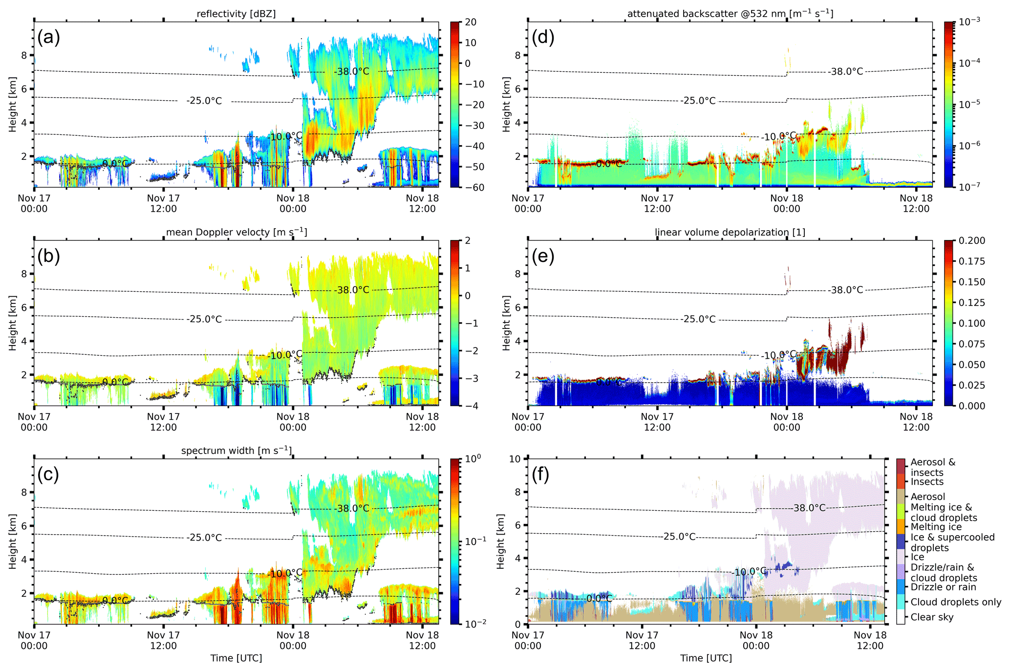
Figure 1 (a) MIRA-35 radar reflectivity factor, (b) radar mean Doppler velocity (middle), (c) radar spectrum width, (d) PollyXT lidar-attenuated backscatter coefficient at 532 nm, (e) PollyXT lidar linear volume depolarization, and (f) Cloudnet target classification of 17 November 2014, 00:00 UTC, to 18 November 2014, 13:30 UTC, observed during the ACCEPT experiment in Cabauw, Netherlands. Black dots (a–c) indicate the first cloud base detected by the ceilometer.

2.2 Description of the used artificial neural network

Luke et al. (2010) use collocated measurements with profiling cloud Doppler radar and polarization lidar in thin mixed-phase clouds or lower layers of thick mixed-phase clouds to provide information about the existence of liquid water in higher cloud layers by predicting the lidar backscatter and depolarization signal from morphological features in the cloud radar Doppler spectrum. The procedure to determine the existence of supercooled liquid droplets from cloud radar Doppler spectra is a two-step technique. In the first step, morphological feature extraction from cloud radar Doppler spectra is done by applying a second-order Gaussian continuous wavelet transform (CWT) to each measured radar Doppler spectrum. In that way, the spectral power is decomposed into a two-dimensional array with feature localization in Doppler velocity and spectrum width; each Doppler spectrum can thus be regarded as a sum of different Gaussians. In the second step, a selected subset of bins from six different scales of the CWT as well as the first three radar moments (reflectivity factor Z_e – dBZ, mean Doppler velocity V_D – m s⁻¹, and Doppler spectrum width σ – m s⁻¹) of each Doppler spectrum is the input to the ANN used in this work to predict the existence of liquid. The ANN is of the multi-layer perceptron (MLP) type consisting of 256 input nodes, five hidden layers, and two output nodes. Each of the five hidden layers consists of 32 nodes. Lidar particle backscatter coefficient (β – sr⁻¹ m⁻¹) and lidar depolarization ratio (δ) are the two output variables from which the existence of liquid is predicted using appropriate thresholds of β and δ later on. In the training phase, which was performed on data from the Mixed Phase Arctic Clouds Experiment (MPACE, Verlinde et al., 2007) obtained in autumn 2004 at the US Department of Energy's (DOE's) Atmospheric Radiation Measurement (ARM) North Slope of Alaska (NSA) permanent site in Utqiagvik (formerly known as Barrow), Alaska, the back propagation of errors algorithm was applied. In short, the β and δ output of the ANN for each time and height pixel were compared to values measured with a high-spectral-resolution lidar (HSRL, Eloranta, 2005). The difference between ANN-predicted and lidar-observed (i.e. the error) was monitored, and the internal weights of the nodes were adjusted until the error did not decrease any further during the successive cycling through the Doppler spectra training data set. Only a fraction of the MPACE data was considered in the training phase: most of the data were used for validation. Turbulent broadening of the cloud radar Doppler spectrum (e.g. in strong convection) decreases the imprint of cloud microphysics on the Doppler spectra. The MPACE data set was characterized by largely stratiform conditions. As stated in Gardner and Dorling (1998), the ability of an ANN to predict cloud properties does not only depend on an informed choice of predictors, but also requires sufficient data that fully represent all cases that the ANN is required to generalize, as ANNs perform well for interpolation but poorly for extrapolation. We can thus only expect good predictions of liquid in low-turbulent clouds but not in strongly convective clouds. The objective of this study was to check the performance of the ANN trained with the MPACE observations in Luke et al. (2010) on a new data set, and the ANN was thus not re-trained.

2.3 Classifying liquid-containing sections from ANN predictions

The ANN predicts backscatter coefficient and particle depolarization ratio. Thresholds need to be applied to these predicted β and δ in order to identify regions which show optical properties similar to the ones produced by liquid water.

For visual illustration of the mapping from predicted lidar variables to hydrometeor class labels, a scatter plot of predicted β and δ was created (Fig. 2a). As previously mentioned, lidar-observed or ANN-predicted high values of β and near-zero δ are reliable indicators of liquid-dominated cloud regions; they clearly stand out as a feature in Fig. 2a. The scatter plot of predicted β and δ shows two more distinct features, one between the functions “linear-1” and “linear-2” with higher values of δ and lower values of β indicating ice and another feature of very high values of δ and very low values of β situated below the function “linear-2” that can be attributed to the optically thinner ice cloud with lower radar reflectivities above 7 km on 18 November 2014 (see Fig. 2b). Similarly to Luke et al. (2010), fixed thresholds of β and δ were used to derive a binary mask separating liquid predictions from other target types. For a sensitivity study of ANN-predicted liquid occurrence for the entire ACCEPT data set, different HSRL-based published thresholds (Shupe, 2007; de Boer et al., 2009; Luke et al., 2010) as well as a new linear function threshold (labelled “linear-1” in Fig. 2) were employed (see Table 1). Threshold values for β of all three published studies are similar. Shupe (2007) and Luke et al. (2010) use the same δ threshold of 0.1 for liquid classification, while de Boer et al. (2009) with a value of 0.03 are much more stringent. The studies are subsequently referred to as “Shupe2007”, “deBoer2009”, and “Luke2010”. The linear-1 threshold function was found by a sensitivity study and gave the most similar classification results to the three cited published threshold values. Figure 2b shows the corresponding time–height representation colour-coded by linear separation of the predicted (backscatter vs. depolarization) dimension using linear functions.

Table 1 Published thresholds of β and δ for lidar-based liquid classification and the linear-1 function threshold used for the ACCEPT data set.

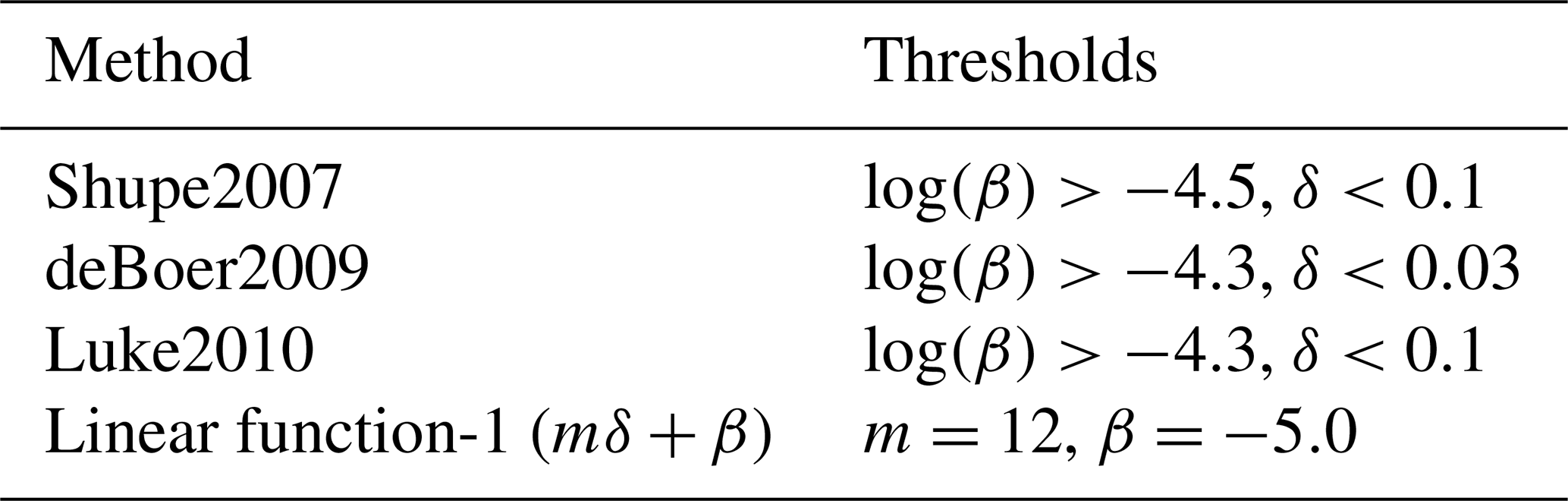
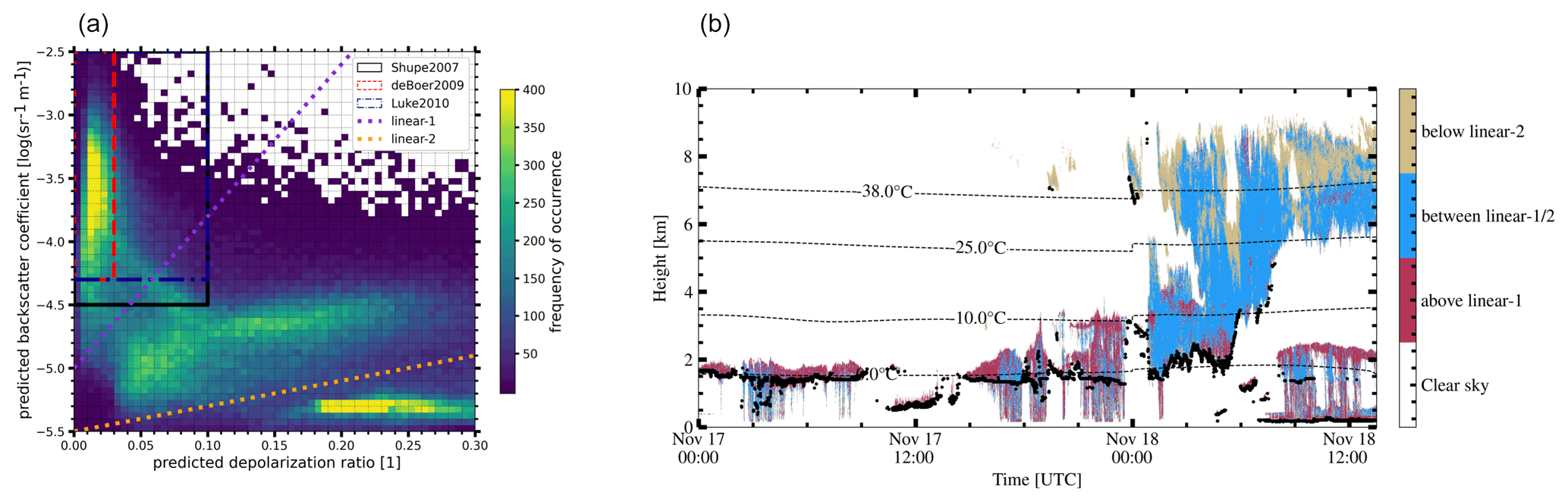
Figure 2 (a) Frequency of occurrence of ANN-predicted lidar backscatter coefficient β vs. predicted lidar linear depolarization δ for the 17–18 November 2014 case study. (b) Time–height mapping of predicted β and δ of the three corresponding areas in the (a) panel, which are separated by the two linear thresholds. Black dots (b) indicate the ceilometer cloud base height.

The liquid classification methods were applied to the entire ACCEPT data set. In doing so, the following pre- and post-processing steps were applied to the 7-week-long data set. Firstly, to account for the effects of radar partial beam filling, cloud edges are excluded from the ANN input data by setting data in the first and last range gates of a detected cloud (i.e. cloud base and cloud top pixel) to “clear sky”. Secondly, pixels classified as aerosols/insects were explicitly excluded. Thirdly, using model temperature data of the Global Data Assimilation System (GDAS1) employed by the Global Forecast System (GFS) model, unphysical liquid predictions below −37 ^∘C were re-classified as ice. The in-cloud pixels which were classified as liquid-containing by the ANN using the above-mentioned thresholds were sometimes quite patchy. Similarly to Shupe (2007), a homogenization step to create more coherent liquid layer structures by using a 5×5 pixel neighbourhood smoothing was introduced. A pixel was kept as a liquid-containing pixel when at least 60 % of the pixels in the 5×5 box around the centre one were also classified as liquid-containing.

3 Results and discussion

To assess the performance of the Luke et al. (2010) ANN-based liquid prediction from cloud radar Doppler spectra using different published thresholds of lidar backscatter coefficient and depolarization ratio against the Cloudnet target classification and against independent observables, a two-step validation was performed. Firstly, a case study (17–18 November 2014 consisting of 100 000 samples) was analysed in depth: see Table 2. Secondly, statistical results for the ANN-based liquid prediction for the entire ACCEPT data set (1070 h of observations, i.e. 1.7 million samples) are given in Table 3 and discussed subsequently. In the following, the abbreviation CD is used for cloud droplet-bearing samples and non-CD for non-cloud droplet-bearing samples. It should be noted that no further distinction between other liquid-bearing samples such as drizzle/rain is made for the ANN-based liquid predictions.

Predictions that meet the criteria from Sect. 2.3 are compared to classifications from Cloudnet (treated as ground truth). The comparison yields an error matrix consisting of correctly classified predictions, i.e. true positive (TP) and true negative (TN) as well as false positive (FP) and false negative (FN), which concern wrong predictions respectively. Described below are four metrics used to evaluate the predictive performance against Cloudnets' liquid detection, three correlation coefficients ρ_a,b, and the fraction of liquid predicted located within a relative humidity above 90 %.

1. Error matrix: a 2-by-2 matrix consisting of the numbers for correctly identified CD (TP) and non-CD (TN) time–height grid cells as well as falsely classified non-CD (FP) and CD (FN) cells respectively, i.e.

   $$\begin{array}{}\text{(1)}& {\displaystyle }\text{EM}=\left(\begin{array}{cc}\mathrm{TP}& \mathrm{FN}\\ \mathrm{FP}& \mathrm{TN}\end{array}\right).\end{array}$$

2. Precision: a real value between 0 and 1, where 1 is the perfect score. prec $=\frac{\mathrm{TP}}{\mathrm{TP}+\mathrm{FP}}$, i.e. the fraction of how many predictions were correctly classified as CD (i.e. TP) by the sum of TP and predictions falsely classified as CD (i.e. FP). In the context of this work, it measures the amount of CD overestimation. The closer precision gets to 1, the more precisely actual CD cells are predicted as such. Precision can also be described as 1 minus the false alarm rate.

3. Recall or probability of detection: a real value between 0 and 1, where 1 is the perfect score. recall $=\frac{\mathrm{TP}}{\mathrm{TP}+\mathrm{FN}}$, i.e. the fraction of TP and the sum of TP and falsely classified non-CD (i.e. FN). In the context of this work, “recall” measures the amount of CD underestimation. The closer recall gets to 1, the less likely it is missing actual CD cells. Note: the ceilometer lidar signal which is used as a ground-truth indicator for CD availability is much more sensitive to CD than Doppler cloud radar signals, and thus recall values below 1 are expected.

4. Accuracy: a real value between 0 and 1, where 1 is the perfect score. acc $=\frac{\mathrm{TP}+\mathrm{TN}}{\mathrm{TP}+\mathrm{TN}+\mathrm{FP}+\mathrm{FN}}$, i.e. the fraction of all correctly predicted CD pixels and the sum of all samples. In the context of this work it measures the overall fraction of correct vs. incorrect predictions, where acc =0.75 if the retrieval correctly classifies three out of four inputs.

5. Correlation between MWR-LWP and retrieved liquid layer thickness LLT: The MWR-LWP time series is correlated with the LLT time series computed as the sum of the vertical extent of CD-containing volumes LLT $=N_{\mathrm{CD}}\cdot \mathit{\delta }h$, with δh=40 m range resolution. Profiles in which rain was observed on the ground were excluded from the correlation coefficient determination to avoid wrong MWR-LWP caused by a wet MWR radome.

6. Correlation between ceilometer first cloud base height (CBH) and retrieved first liquid layer height (LLH): the ceilometer first CBH time series is correlated with the first LLH time series as retrieved from the CD mask.

3.1 17–18 November 2014 case study results

The 37.5 h-long case study of 17 November 2014, 00:00 UTC, to 18 November 2014, 13:30 UTC, was characterized by a multitude of cloud types, including pure liquid-water clouds, stratiform mixed-phase clouds, high clouds, mid-level clouds and near-surface clouds (fog) as shown in Fig. 1. On 17 November 2014 between 03:00–09:00 UTC and 15:00–24:00 UTC several rain showers from low mixed-phase clouds with cloud top temperatures between −10 and −2 ^∘C were observed. At around 12:00 UTC, a thin warm liquid cloud at 1 km altitude with a LWP below 30 g m⁻² was present. On 18 November, different multi-layer clouds with varying vertical extents were present, a high cloud at 6–9 km was firstly situated above a mid-level cloud at 2–5 km and later on over a precipitating stratiform cloud at about 2 km altitude with a cloud top temperature of −5 ^∘C. Below this cloud was a layer of near-surface fog.

Figure 3 Sensitivity study of liquid pixel classifications of the 17–18 November 2014 case study using liquid mask thresholds of Shupe2007 (a), deBoer2009 (b), Luke2010 (c), and linear-1 (d) on the ANN-predicted lidar variables. Light brown: Cloudnet-only liquid classifications, blue: ANN-predicted pixels using the given thresholds which were not classified as liquid droplets by Cloudnet, red: pixels classified as liquid by the ANN and Cloudnet, grey shading: pixels for which neither Cloudnet nor the ANN classified cloud droplets, black dots: ceilometer first cloud base height, and white: clear sky.

In Fig. 3 the comparison of the resulting liquid masks of the ANN of all presented thresholds and for Cloudnet for this case study are shown. There is mostly good agreement in liquid detection for the stratiform mixed-phase clouds on 17 November before 21:00 UTC and the liquid cloud at around 12:00 UTC on 17 November. However, since the liquid-threshold boundaries of deBoer2009 are very strict, many potential liquid pixel candidates are not considered (e.g. around 03:00 UTC and 18:00 UTC on 17 November). For this particular case, the Cloudnet target classification algorithm was not able to fully identify the cloud top layer at −10 ^∘C during 21:00–24:00 UTC on 17 November and at about 2 km during 09:00–12:00 UTC on 18 November as mixed-phase and/or supercooled liquid-containing because of full lidar signal attenuation in the rain/fog below. The ANN-based liquid detection clearly outperforms Cloudnet in these situations.

For independent validation of the areas classified as liquid-containing, the summed-up liquid layer thickness (LLT) of all pixels classified as liquid by the ANN or Cloudnet is compared to the MWR-LWP (Fig. 4) as proposed by Luke et al. (2010). MWR-LWP uncertainty amounts to 25 g m⁻². Profiles in which considerable amounts of rain/drizzle reached the ground were excluded in the LLT determination to avoid situations with a wet MWR radome, leading to an invalid MWR-LWP estimate (as indicated by the rain flag in Fig. 4). In some situations the ANN and in others Cloudnet match the time series of MWR-LWP better. A large discrepancy between ANN-LLT and MWR-LWP is obvious on 18 November, 04:00–06:00 UTC: MWR-LWP is very low, while ANN-LLT is high. A misclassification of ice as liquid by the ANN at 2–3.5 km height can thus be concluded which is corroborated by the PollyXT lidar signal showing high depolarization values indicating ice crystals. After 07:00 UTC on 18 November, the lidar signals are fully attenuated by the fog near the ground and are thus not available for assessment of ANN classifications in higher layers. Analysis of radar Doppler spectra time and height spectrograms at around 6–9 km altitude showed only monomodal spectra related to the falling ice crystals from above. In conclusion, most certainly, no formation of supercooled liquid at 7 km altitude at −37 ^∘C occurred. The ANN thus most likely misclassified ice as liquid because the observed Doppler spectra at around 7 km were characterized by high spectrum width, small reflectivities and small mean Doppler velocities. High Doppler spectrum width might be related to more turbulent conditions which result in a decrease in the performance of the ANN because the microphysical imprint of the hydrometeors on the radar Doppler spectra is decreased.

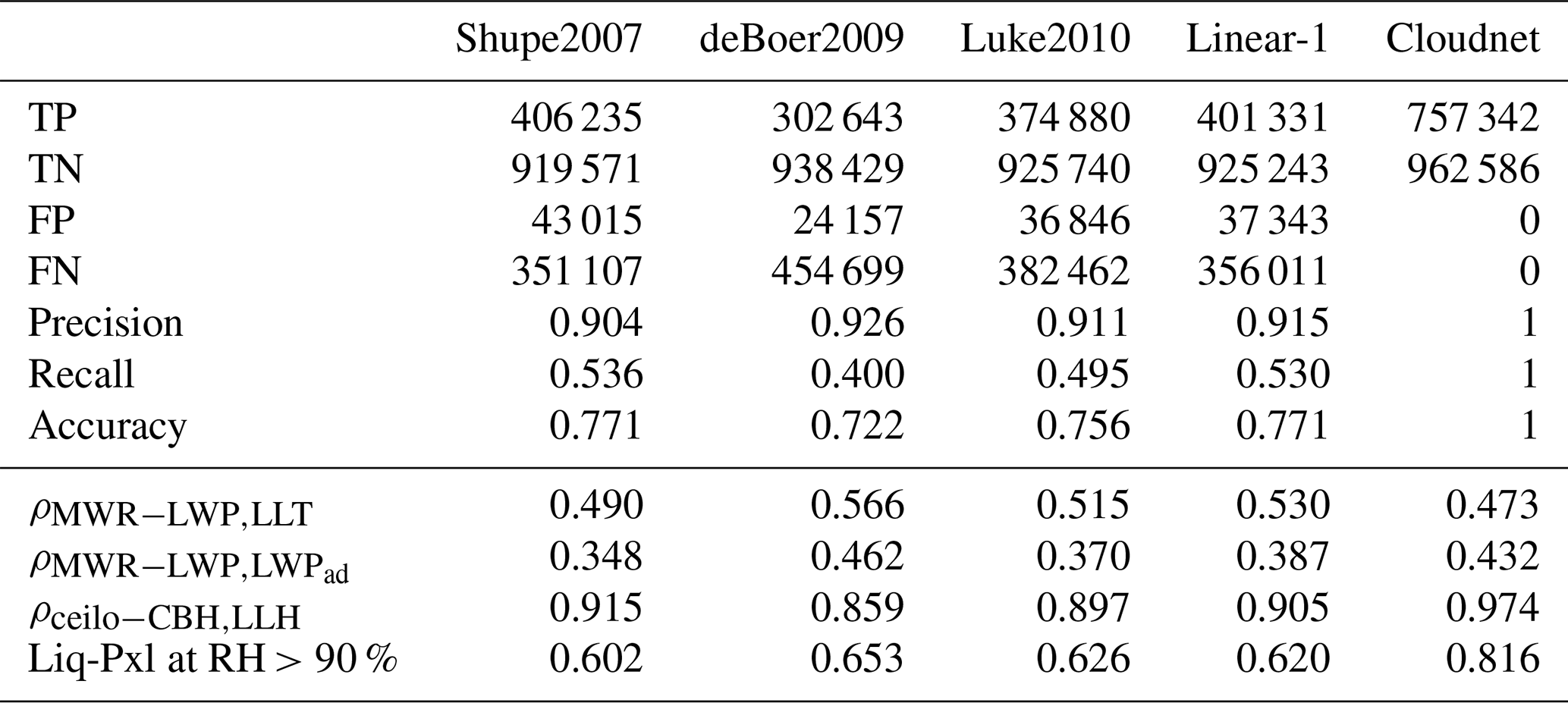
Table 2 Error matrix, performance metrics, and correlation coefficients for MWR-LWP vs. LLT, MWR-LWP vs. LWP_ad, and ceilometer CBH vs. LLH, case study 17–18 November. The statistic includes only valid pixels.

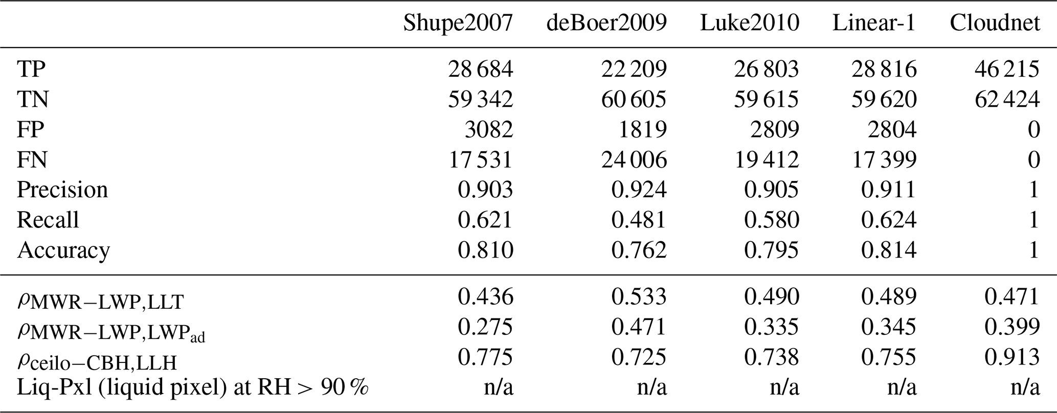
n/a: not applicable

The error matrix and evaluation metrics (first eight rows in Table 2) show the performance of the ANN by comparing ANN-based liquid predictions to valid Cloudnet liquid detections for time–height cells with reliable radar and lidar signal status. Depending on the threshold given in Table 1, precision ranges between 0.9 (Shupe2007) and 0.92 (deBoer2009). Contrarily, recall values range between 0.53 (deBoer2009) and 0.67 (linear-1), indicating that looser thresholds are better at detecting more TPs while keeping the number of FNs comparably low. Overall accuracy ranges between 0.76 (deBoer2009) and 0.81 (linear-1). Regions with high Doppler spectrum width near the cloud base (see Fig. 1, 18 November, 03:00–06:00 UTC between 2 and 3 km altitude) contribute a large portion of those FPs for all thresholds. Lower recall values indicate a higher degree of underestimation of CD detections, which is caused by liquid layers with low LWP values below 50 g m⁻², e.g. the thin liquid cloud on 17 November around 12:00 UTC at 0.5 to 1 km altitude. Profiles characterized by low precipitation rates of rain and drizzle have a negative Cloudnet rain flag and are thus not excluded from the analysis. For these drizzle/rain pixel the ANN often predicts liquid (see Figs. 3 and A2 between 0 and 1.5 km). Since the ANN does not distinguish between different liquid classes such as drizzle/rain and cloud droplets (CDs), the ANN classifies all these pixels as cloud droplets, which are then counted as FPs. FNs often occur when Cloudnet classifies a certain hydrometeor class at low altitude and extends this target class for all pixels in the profile up to the cloud top, which e.g. either happens in low-intensity precipitation (see Fig. A1, misclassification of drizzle/rain as cloud droplets by Cloudnet, e.g. 17 November 2014, 03:00–04:00 UTC, 0.5–2 km) or for the ice and supercooled droplets class on 17 November, 17:30 UTC, resulting in a 1 km-deep mixed-phase layer at 1.5–2.5 km altitude. In such situations the ANN might be more accurate in determining the location of cloud droplets, but since it is evaluated against Cloudnet as a ground truth, FNs result.

In this work the ceilometer first CBH is correlated with the predicted first LLH. ${\mathit{\rho }}_{\mathrm{ceilo}-\mathrm{CBH},\mathrm{LLH}}$ of the four ANN methods are on the order of 0.86 (deBoer2009) to 0.92 (Shupe2007) for the entire ACCEPT data set (see Table 3); i.e. there is a failure rate of 8 %–14 %. This failure rate can be explained by several conditions. Firstly, in some situations, like on 18 November 2014 between 01:00 and 04:00 UTC, the ceilometer cloud base variable is not representing the base of the liquid layer but instead the base of precipitating ice crystals (Fig. 1). This is caused by specular reflection from the planar planes of horizontally aligned ice crystals as described in Westbrook et al. (2010). When the ANN is not misclassifying these ice crystals as liquid, the difference in ceilo-CBH and ANN-LLH is high. Secondly, there are situations where liquid layers with low LWP are only detected by the ceilometer but not by the cloud radar (17 November, 11:00 UTC, cloud at 1.7 km). Thirdly, there are cloud scenes where the ceilometer is fully attenuated by precipitation or low-level fog (thus reporting the precipitation or fog base as first cloud base) which the radar can penetrate/is not sensitive to or which is below the first radar range gate. Fourthly, in situations where the ceilometer is still able to penetrate light precipitation to detect CBH (17 November, 03:00–09:00 UTC, 17:00–24:00 UTC) and the ANN misclassifies drizzle/rain as cloud droplets, further discrepancies arise. These conditions lead to a decrease in the ${\mathit{\rho }}_{\mathrm{ceilo}-\mathrm{CBH},\mathrm{LLH}}$. The ${\mathit{\rho }}_{\mathrm{ceilo}-\mathrm{CBH},\mathrm{LLH}}$ for ceilometer CBH and Cloudnet for the entire ACCEPT data set is higher and amounts to 0.97. While the liquid layer base height variable in Cloudnet is based on the gradient of the ceilometer-attenuated backscatter coefficient, the internal ceilometer cloud base determination is not precisely documented in the ceilometer manual. Differences in cloud base height leading to a failure rate of 3 % may thus occur due to different backscatter coefficient thresholds.

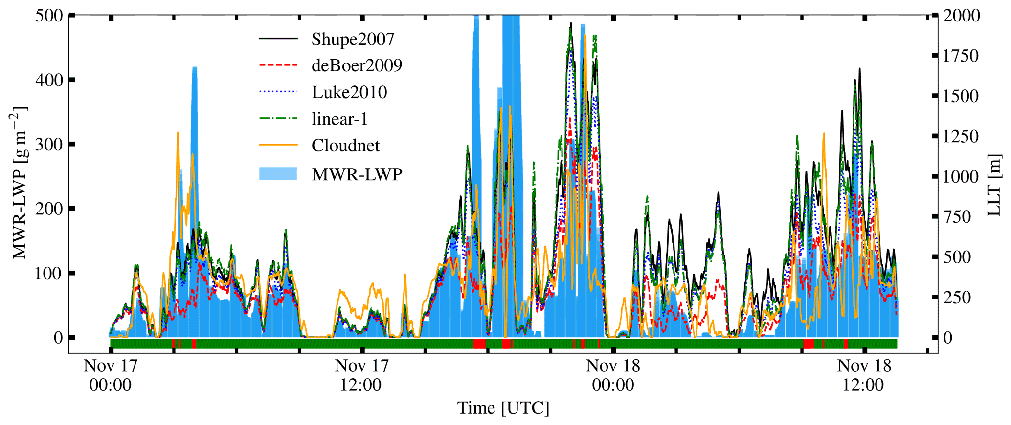
Figure 4 Comparison of MWR-LWP (left y axis, blue bars) and liquid layer thickness (LLT, right axis) of the ANN-predicted liquid layer masks and Cloudnet LLT (orange) for the 17–18 November 2014 case study for all used liquid-detection thresholds. The disdrometer-based Cloudnet rain flag is depicted by green and red markers near the bottom of the plot respectively, indicating profiles with rain (red) and times where it was drizzle-/rain-free or precipitation rates were too low to be observed by the disdrometer.

The ${\mathit{\rho }}_{\mathrm{MWR}-\mathrm{LWP},\mathrm{LLT}}$ also shows positive correlations for all the methods. As shown in Table 2, it ranges between 0.44 (Shupe2007) and 0.53 (deBoer2009); for Cloudnet the ${\mathit{\rho }}_{\mathrm{MWR}-\mathrm{LWP},\mathrm{LLT}}$ amounted to 0.47. Converting the LLT to the physically more meaningful LWP_ad,cor results in ${\mathit{\rho }}_{\mathrm{MWR}-\mathrm{LWP},{\mathrm{LWP}}_{\mathrm{ad}}}$ that are very similar to ${\mathit{\rho }}_{\mathrm{MWR}-\mathrm{LWP},\mathrm{LLT}}$, with moderate correlation (0.47) for deBoer2009 and weaker correlations for all the other methods. Both ${\mathit{\rho }}_{\mathrm{MWR}-\mathrm{LWP},\mathrm{LLT}}$ and ${\mathit{\rho }}_{\mathrm{MWR}-\mathrm{LWP},{\mathrm{LWP}}_{\mathrm{ad}}}$ of deBoer2009 show the strongest relationship with the measured MWR-LWP. The period 17 November, 21:00 UTC, to 18 November, 12:00 UTC, in Fig. 4 shows the highest differences in LLT between the deBoer2009, Cloudnet, and other methods. The number of CD predictions in the precipitating system (17 November, 20:00–23:00 UTC), the region with higher spectrum width (18 November, 04:00–06:00 UTC, at the cloud base and 18 November, 10:00–13:00 UTC, at 7 km altitude; see Fig. 3) is lowest for deBoer2009, therefore reflecting the MWR-LWP best. However, deBoer2009 also counts the least number of TPs, due to its tight thresholds, which seems to have minor effects on the correlation coefficient. Unfortunately, no radiosondes were launched during the presented case study, so the relative humidity-related measure could not be determined. Multiple other case studies had similar results.

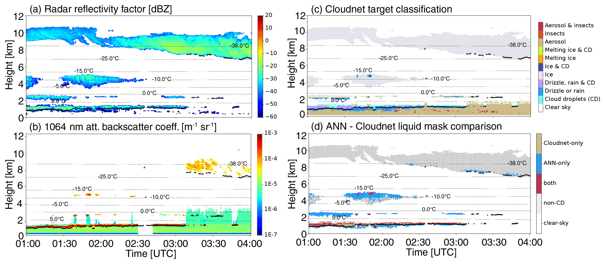
Figure 5 Observations and retrievals on 5 October 2014, 01:00–04:00 UTC: (a) MIRA-35 radar reflectivity factor, (b) PollyXT 1064 nm attenuated backscatter coefficient, (c) Cloudnet target classification, and (d) comparison of Cloudnet and ANN liquid masks. The first ceilometer cloud base is indicated by black dots.

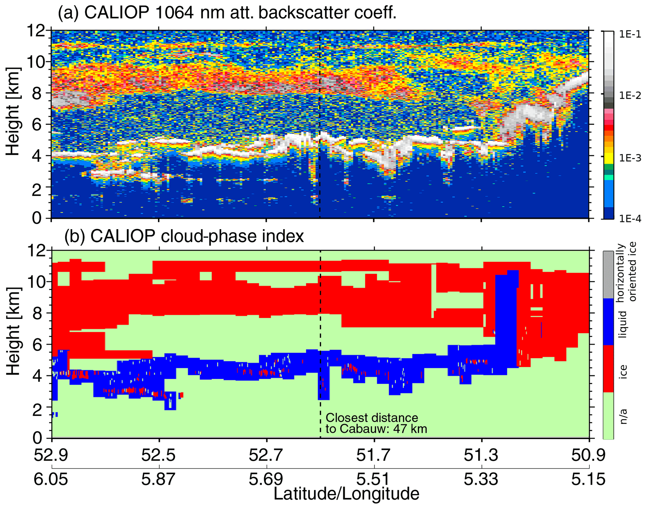
Figure 6 (a) Curtain plots of CALIOP 1064 nm attenuated backscatter coefficient and (b) CALIOP cloud-phase index on 5 October 2014 where the closest distance of CALIPSO to Cabauw was 47 km at 01:05 UTC.

3.2 5 October 2014 case study results

As previously mentioned, no validation of the ANN liquid prediction can be made if the ground-based lidar signals are fully attenuated. We therefore use the unique opportunity to compare the Cloudnet and ANN liquid identifications in multi-layer cloud situations to a nearby (47 km distant) CALIPSO overpass on 5 October 2014, 01:05 UTC. On 5 October 2014, 01:00–04:00 UTC, multiple cloud layers were present. Besides warm stratiform liquid clouds below 3 km altitude, a mid-level cloud with a cloud top temperature of −14 ^∘C was observed at 5 km altitude. An extensive cirrus was present between 7 and 10.5 km altitude. From 01:00 to 03:00 UTC, the PollyXT lidar signal was mostly fully attenuated by the lowest liquid cloud at 1 km altitude, leading to a misclassification of liquid as ice by Cloudnet for the warm cloud at 2.5 km altitude. Also (except for a few pixels where the lidar had a valid signal), Cloudnet classified the mid-level cloud as ice cloud. The ANN correctly predicted liquid for all warm clouds (note that below the cloud base of the lowest cloud layer, ANN also predicts liquid which is counted as CDs) since it does not distinguish between different liquid classes such as cloud droplets and rain/drizzle. The ANN classifies the mid-level cloud as liquid-topped with ice precipitating from it below. The phase classification of the ANN in the cirrus is mostly ice except for some regions close to the cloud base, where high spectrum width and near-zero mean Doppler velocities result in a prediction of supercooled liquid.

The cloud fields were extensive, so CALIPSO identified a very similar cloud situation with a cirrus of high vertical extent and a mid-level cloud at 3.5–5 km. The CALIOP signal was fully attenuated in this cloud layer, so the low-level warm clouds were missed by the satellite observation. The CALIPSO cloud-phase index classified the high cloud as ice cloud and the mid-level cloud as liquid-topped cloud with liquid-only or liquid + ice in the lower regions of this cloud. CALIPSO thus validates the ANN-based liquid prediction for the mid-level cloud. This points to the usefulness of employing satellite-based hydrometeor target classifications as an independent validation tool.

3.3 Statistical results for the entire ACCEPT field campaign

A more general evaluation of all methods is done for the entire ACCEPT field campaign comprised of 1070 h of observations counting more than 1.7 million samples. The summary of this evaluation is presented in Table 3. All ANN thresholds achieve high precision values >0.9, indicating a low FP rate. Recall values are moderately lower compared to the 17–18 November 2014 case study, ranging from 0.4 (deBoer2009) to 0.54 (Shupe2007). Accuracy lies above 0.75 (three out of four predictions are correct) for all methods except slightly lower values for deBoer2009 (explained in Sect. 3.1). However, deBoer2009 achieves the best correlation for ${\mathit{\rho }}_{\mathrm{MWR}-\mathrm{LWP},\mathrm{LLT}}$ and ${\mathit{\rho }}_{\mathrm{MWR}-\mathrm{LWP},{\mathrm{LWP}}_{\mathrm{ad}}}$, due to CD overestimation (larger numbers of FPs) for Shupe2007, Luke2010, and linear-1. Overall, all the methods achieve better correlation values for the entire data set compared to the case study of 17–18 November 2014, with high ${\mathit{\rho }}_{\mathrm{ceilo}-\mathrm{CBH},\mathrm{LLH}}$, values ranging from (0.86–0.92) to (0.97) for Cloudnet respectively. The similar values of correlation coefficients and cloud droplet prediction error matrix elements in Tables 2 and 3 indicate that the entire data set is well represented by the 17–18 November 2014 case study. As indicated in Sect. 3.1, misinterpreted spectral signatures (small ice particles with low fall speed are misclassified as liquid) and turbulence-broadened radar Doppler spectra are the main driver of misclassifications of the pre-trained Luke et al. (2010) approach.

Table 3 Error matrix, performance metrics, and correlation coefficients for ceilometer CBH vs. LLH, MWR-LWP vs. LLT, and MWR-LWP vs. LWP_ad,cor for the entire ACCEPT data set. The statistic includes only valid pixels.

An additional independent validation is done using radiosonde launches from the campaign site as well as launches from DeBilt airport about 30 km away. Liquid-detected pixels are only evaluated in this way within ±30 min of a radiosonde launch, meaning only a small subset of data from the entire field experiment is considered. Radio sounding profiles with relative humidity (RH) with respect to liquid water (w.r.t.l.) larger than 90 % overlapping with liquid detection layers occur only during 1.5 h out of 58 h of available liquid detection data; i.e. only during 2.5 % of the time is liquid classified. This validation method thus only has very limited utility for the quality of the thermodynamic-phase classifications made but is shown here for the sake of completeness as similar future evaluation studies might have larger data sets available. As shown in the last row of Table 3, for all methods the majority of the number of liquid-containing pixels occur when the radiosonde RH w.r.t.l. is larger than 90 % and liquid occurrence is thus likely. There are two explanations why the fraction of Cloudnet-classified liquid pixel overlapping with areas of radiosonde RH >90 % is much higher (72 %) than for the ANN results (54 %–61 %). Firstly, with the radiosonde drifting away with height (and time), the assumption of having the same thermodynamic profile over the ACCEPT site and the sounding location becomes less certain for liquid detections higher in the atmospheric profile (where the ANN is predicting more liquid than Cloudnet). Secondly, not all elements of the error matrix are represented in the overlap fraction of the pixel with liquid detection and RH >90 %: while liquid pixels unrecognized by Cloudnet (i.e. beyond lidar attenuation) are not included in the overlap fraction, wrongly detected ANN liquid pixels (i.e. FPs) are included and thus reduce the fraction of overlap pixels for ANN-predicted liquid.

To understand the performance of the liquid prediction by the ANN more in depth, conditions under which enhanced spectrum width values lead to liquid-prediction error matrix elements TP, FP, and FN are described subsequently. The co-existence of multiple hydrometeor types with sufficiently different fall velocities in the same radar volume leads to multi-modal Doppler spectra with a high total spectrum width. If the slow-falling hydrometeors have a low reflectivity and narrow peak width, the ANN likely predicts liquid. If there are indeed small cloud droplets and larger ice crystals in the volume, this results in TPs. If however there is a co-existence of multiple ice crystal types of which one is small and has a small fall velocity, this results in FPs. Furthermore, if the enhanced spectrum width (SW) is not caused by multiple hydrometeor types but by turbulence, liquid peak signatures can be smeared, thus leading to FNs. Under calm conditions (low turbulence) it is more likely that a bimodal Doppler spectrum with two ice classes is misclassified as one ice and one liquid class, leading to FPs. This problem diminishes with increasing turbulence because of broadening of the peaks and smearing of the individual peaks. The latter (smearing) is the same mechanism for FNs under high turbulent conditions.

However, considering only spectrum width is not sufficient as it is always a combination of radar reflectivity, mean Doppler velocity, spectrum width, etc., that leads to correct or incorrect classification of liquid by the ANN. By discussing relative frequency of occurrence (FoO) plots of radar moments and environmental temperature of the liquid-prediction error matrix elements TP, TN, FP, and FN as illustrated in Fig. A3 in the Appendix, we assess which combinations of moments mostly lead to TPs. As shown in Fig. A3, the distribution of radar moments of TPs is different from those of TNs, FPs, and FNs, while the FoO distribution of radar moments of the latter (TNs, FPs, FNs) are mostly similar. Specifically, the radar reflectivities of TPs of cloud droplets is monomodal with a maximum FoO at −25 to −30 dBZ, while it is bimodal for TNs, FPs, and FNs, with the two maxima occurring at −25 and −10 dBZ. The second maximum at −10 dBZ can be attributed to situations in which the ANN predicted cloud droplets in drizzle/rain. With values between −2 and 0.5 m s⁻¹, the distribution of mean Doppler velocities of TPs is narrower than of TNs, FPs, and FNs, which have V_D values between about −4 and 1 m s⁻¹ and a maximum FoO at more negative values of around −0.5 m s⁻¹ than the TPs (maximum FoO at −0.2 m s⁻¹). TPs generally occur at larger spectrum width σ than TNs, FPs, and FN, with a maximum FoO of TPs at 0.2–0.25 m s⁻¹, while the FoO of TNs, FPs, and FNs peaks at 0.05–0.1 m s⁻¹. Spherical particles have a theoretical radar linear depolarization ratio (LDR) of minus infinity dB; however, due to technical limitations, the smallest detectable LDR of the MIRA cloud radar is −30 dB, which corresponds to the peak of FoO of TPs. While FN also peaks at −30 dB, TN and FP are characterized by high FoO in the range of −30 to −25 dB, which again can be attributed to drizzle/rain, where perfect sphericity of the hydrometeors is not always given. The FoO distributions of error matrix elements in the environmental temperature space show that only a considerable fraction of TNs are detected at very low temperatures, which is plausible. Maximum FoO of all four error matrix elements occurs at positive temperatures, which is caused by the consecutive attenuation of the ground-based lidar signal with height, leaving more pixels at higher temperature in the Cloudnet–ANN comparison. Comparing the FoO of the liquid detection error matrix with respect to the different backscatter and depolarization thresholds (Shupe2007, deBoer2009, Luke2010, and linear-1), the more stringent criteria of deBoer2009 generally lead to narrower FoO distributions of TPs. Summarizing, as shown in the description of FoO of the radar moments of the error matrix components above, TPs are mostly characterized by high spectrum width in combination with low absolute values of V_D and small radar reflectivities, but due to the overlap of radar moments of all error matrix elements, the same combination of Z_e, V_D, and σ can be caused by TPs, TNs, FPs, and FNs.

4 Summary and outlook

The current study shows that synergistic observations of depolarization lidar and cloud Doppler radar in conjunction with machine learning techniques can be used to detect liquid beyond full lidar signal attenuation. This approach performs well in stratiform cloud situations but is not suited for situations in which the imprint of different hydrometeor populations in the same cloud volume on the cloud radar Doppler spectrum is masked, e.g. by turbulent spectrum broadening. We demonstrated that the ANN of Luke et al. (2010) pre-trained with the MPACE data set in Alaska could successfully be applied to the ACCEPT data set obtained in Cabauw, Netherlands, and is able to improve the Cloudnet target classification for stratiform optically thick liquid layers or situations in which multiple liquid layers exist. We applied different published lidar-based liquid-detection thresholds to the predicted lidar backscatter coefficients and depolarization lidars – all were found to perform better in some situations than others and could be seen as either too stringent (deBoer2009), missing thinner liquid layers, or too broad (Shupe2007, Luke2010, linear-1), leading to misclassifications of ice as liquid. No suggestion on best thresholds can thus be made. To overcome limitations due to ambiguities caused by thresholding, focus should therefore be put on the development of techniques which do not rely on explicit lidar thresholds for liquid detection. This could be realizable by applying novel convolutional artificial neural networks which could be used to exploit the full information content of high-resolution cloud radar Doppler spectra. Additionally, radar Doppler spectra peak-separation techniques such as PEAKO (Kalesse et al., 2019) and peakTree (Radenz et al., 2019) are helpful for assessing the possibilities of liquid occurrence.

Furthermore, two recent studies also showed the benefit of distinguishing between cloud top liquid-bearing layers and embedded liquid layers when assessing the performance of liquid-detection retrievals (Silber et al., 2020; Kalogeras et al., 2021). Silber et al. (2020) retrieved the cloud thermodynamic phase of Arctic clouds based on 1-year zenith-pointing Ka-band radar and HSRL observations. They found that cloud top liquid-bearing samples can be more reliably detected than embedded liquid layers as the latter are more difficult to separate from falling ice signatures in the probability density function (PDF) of the first three radar moments as well as Doppler spectrum left slope and right slope. Kalogeras et al. (2021) developed a Ka-band radar-only, moment-based technique for supercooled liquid-water detection in Arctic mixed-phase clouds. The novelty of this method is that it is a neighbourhood-dependent algorithm employing gradients of moments. They concluded that the best skill levels for liquid detection are realized for combinations of spectral width and reflectivity vertical gradient and also found their algorithm to be most reliable when applied to cloud tops.

The identification of the presence of liquid layers in the entire vertical column of optically thick or multi-layered cloud situations is a first step in getting a better understanding of which microphysical particle growth processes might occur in a mixed-phase cloud. The shown results will therefore be used in follow-up studies for characterization of microphysical hydrometeor growth processes.

Appendix A

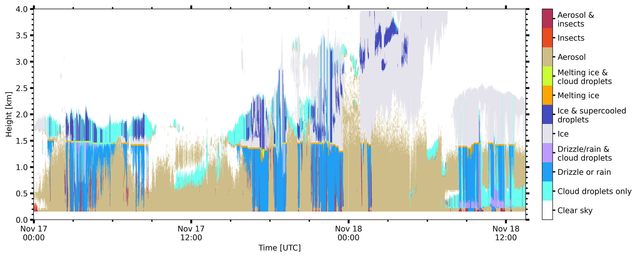
Figure A1 Zoom of Cloudnet target classification from 0 to 4 km altitude for the 17–18 November 2014 case study in Cabauw, Netherlands.

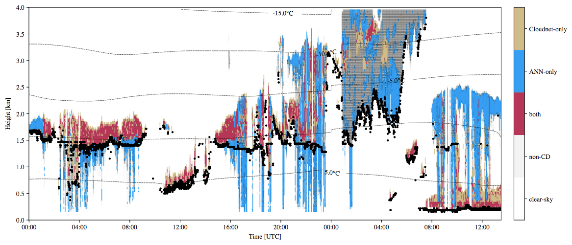
Figure A2 Zoom of comparison of cloud droplet detection of Cloudnet and ANN (using linear-1 thresholds) from 0 to 4 km altitude for the 17–18 November 2014 case study in Cabauw, Netherlands. Black dots indicate ceilometer first cloud base height.

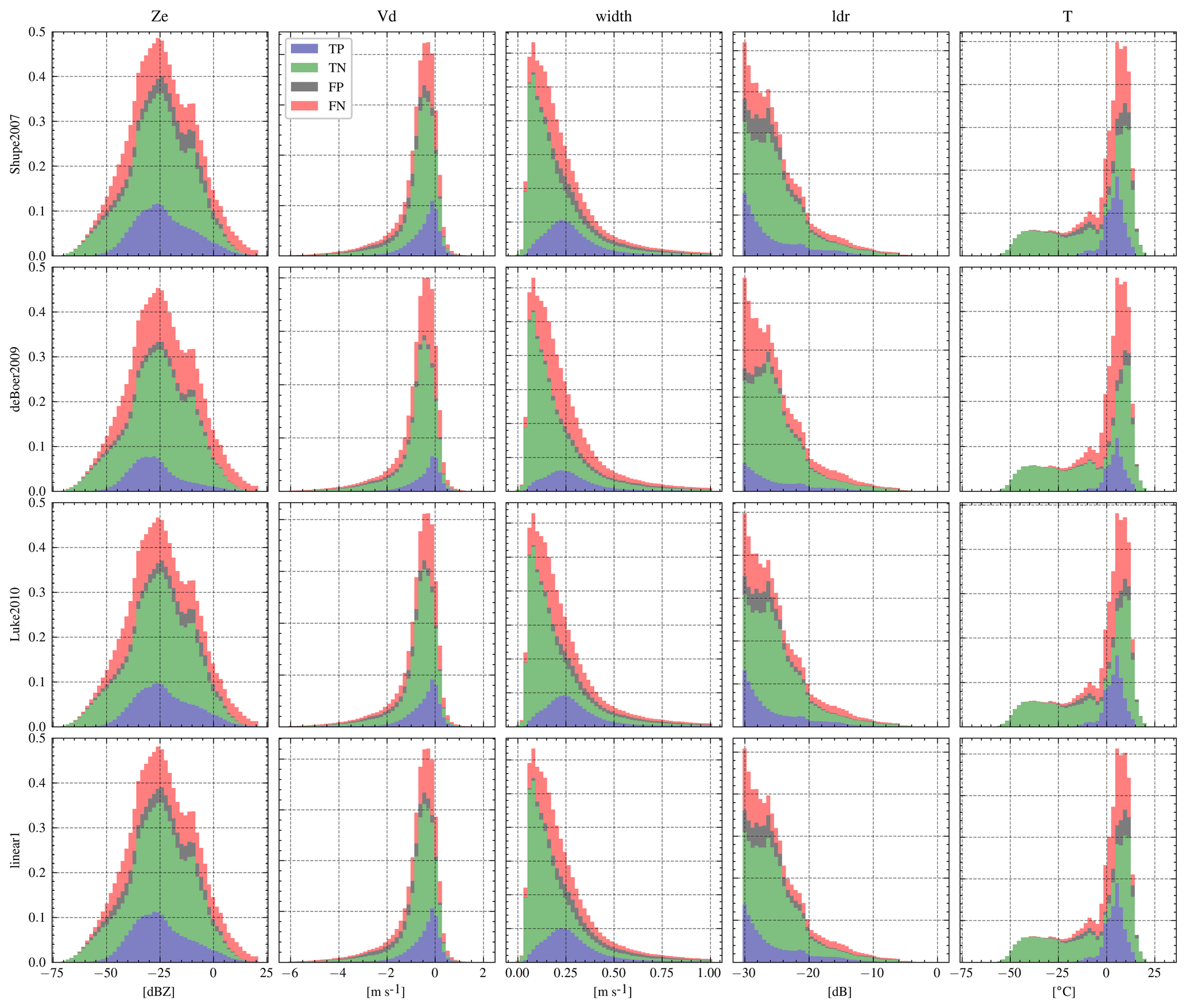
Figure A3 Relative frequency of occurrence plots of radar moment reflectivity (Z_e, left column), mean Doppler velocity (V_d, second left column), spectrum width (middle column), linear depolarization ratio (LDR, second to right column), and environmental temperature T (right column) of ANN liquid-prediction error matrix elements TP (blue), TN (green), FP (grey), and FN (red) for the four utilized ANN-lidar variable thresholds of Shupe2007 (first row), deBoer2009 (second row), Luke2010 (third row), and linear-1 threshold (fourth row) for the entire ACCEPT field experiment.