the Creative Commons Attribution 4.0 License.
the Creative Commons Attribution 4.0 License.
 | 09 May 2022
Metrology for low-cost CO2 sensors applications: the case of a steady-state through-flow (SS-TF) chamber for CO2 fluxes observations
Josep-Anton Morguí
Armand Kamnang
Lídia Cañas
Arturo Vargas
Claudia Grossi
Soil CO2 emissions are one of the largest contributions to the global carbon cycle, and a full understanding of processes generating them and how climate change may modify them is needed and still uncertain. Thus, a dense spatial and temporal network of CO2 flux measurements from soil could help reduce uncertainty in the global carbon budgets.
In the present study, the design, assembly, and calibration of low-cost air enquirer kits, including CO2 and environmental parameters sensors, is presented. Different types of calibrations for the CO2 sensors and their associated errors are calculated. In addition, for the first time, this type of sensor has been applied to design, develop, and test a new steady-state through-flow (SS-TF) chamber for simultaneous measurements of CO2 fluxes in soil and CO2 concentrations in air. The sensors' responses were corrected for temperature, relative humidity, and pressure conditions in order to reduce the uncertainty in the measured CO2 values and of the following calculated CO2 fluxes based on SS-TF. CO2 soil fluxes measured by the proposed SS-TF and by a standard closed non-steady-state non-through-flow (NSS-NTF) chamber were briefly compared to ensure the reliability of the results.
The use of a multiparametric fitting reduced the total uncertainty of the CO2 concentration measurements by 62 %, compared with the uncertainty that occurred when a simple CO2 calibration was applied, and by 90 %, when compared to the uncertainty declared by the manufacturer. The new SS-TF system allows the continuous measurement of CO2 fluxes and CO2 ambient air with low cost (EUR ∼1200), low energy demand (<5 W), and low maintenance (twice per year due to sensor calibration requirements).
- Article
(3089 KB) - Full-text XML
- BibTeX
- EndNote


Global soils store at least twice as much carbon as Earth's atmosphere (Oertel et al., 2016; Scharlemann et al., 2014) and act as sources and/or sinks for greenhouse gases (GHGs) such as carbon dioxide (CO2), methane (CH4), and nitrous oxide (N2O). The total global emission of CO2 from soils is recognised as being one of the largest contributions in the global carbon cycle and is, among others, temperature dependent (Bond-Lamberty and Thomson, 2010a). However, soil respiration is probably the least well constrained component of the terrestrial carbon cycle (Bond-Lamberty and Thomson, 2010b; Schlesinger and Andrews, 2000), and the degree to which climate change will stimulate the soil-to-atmosphere CO2 flux remains highly uncertain (Pritchard, 2011). Continuous measurements of soil fluxes are therefore essential to understand changes in the soil respiration of ecosystems in relation to climate variables such as the atmospheric temperature. A high temporal and spatial resolution monitoring of CO2 fluxes at sensitive areas could offer useful data for a better understanding of the processes at the sources and sinks and thus improve biogenic models (Agustí-Panareda et al., 2016; Randerson et al., 2009). In addition, a complete uncertainty budget of the CO2 flux measurements will be essential for the evaluation and correction of global flux models and their associated uncertainties.
Gas interchange between the soil and the lower atmosphere is generally measured as the quantity of gas exhaled from the soil per unit of surface and time (). It can be measured with different techniques, with the most common being the steady-state through-flow (SS-TF), also known as the open dynamic chamber, and the non-steady-state non-through-flow (NSS-NTF) or closed chamber (Pumpanen et al., 2004). In both cases, the CO2 fluxes are measured using a chamber installed on the soil surface. NSS-NTF measurements are based on the rate of CO2 concentration increase within the chamber, while, in the SS-TF technique, the CO2 efflux is continuously calculated as the difference between the CO2 concentration at the inlet and the outlet under a determined hypothesis (Livingston and Hutchinson, 1995). In the case of NSS-NTF flux measurements, calibrated data are not strictly necessary, as long as the sensor's calibration does not change during the measurement time span because the flux is proportional to the slope of the CO2 concentration increase within the chamber. SS-TF-based results need highly accurate calibration sensors because the absolute values of the measured CO2 concentrations into the chamber are used. A literature survey suggests that, generally, NSS-NTF may underestimate CO2 fluxes by 4 %–14 %, and this is probably due to (i) advective fluxes forced by small pressure gradients between the air into the chamber and outside it and (ii) setting configurations, such as the installation depth of the chamber into the soil. No significant difference was observed when fluxes were measured using SS-TF chambers where no pressure gradients are created (Pumpanen et al., 2004; Rayment, 2000).
In recent years, wireless sensor networks (WSNs) are increasingly used for real-time and high-spatial-resolution monitoring (Oliveira and Rodrigues, 2011). A WSN is composed of spatially distributed autonomous sensors to monitor the physical, chemical, or environmental conditions and to cooperatively pass their data through the network to other locations. WSNs can be used for local data recording for later analysis or for continuous transmission in real time to a remote laboratory for synchronous analysis.
So far, low-cost sensors for CO2 atmospheric measurements have been largely used in industrial environments and for indoor air quality and ventilation rate studies (Fahlen et al., 1992; Mahyuddin and Awbi, 2012; Schell and Int-Hout, 2001). When low-cost sensors are applied at high CO2 concentration areas and/or spots where air concentrations observed are of the order of thousands of parts per million (ppm), the total uncertainty of the measurement does not affect the quality of the study of the concentration variability under different conditions or sources/sinks. However, in the last decade, the improvement in the precision and the decrease in cost of non-dispersive infrared (NDIR) CO2 sensors have made them more useful for multiple purposes (Yasuda et al., 2012). Their low weight and dimensions allow for their utilisation in a wide variety of applications, including unoccupied aerial vehicles (Kunz et al., 2018), CO2 measurement network areas (Kim et al., 2018; Song et al., 2018), and for the study of the distribution of CO2 in large regions, as in the case study of Switzerland (Müller et al., 2020). In order to be able to use these sensors in the outdoor atmosphere, a metrological effort is needed to (i) ensure a traceable and stable calibration, (ii) evaluate and correct the influence of the environmental parameters, such as temperature, relative humidity, and pressure, on the sensor response, and (iii) estimate the total uncertainty related with the sensor calibrations and corrections.
This work presents a low-cost air enquirer kit, including NDIR CO2 and environmental parameters sensors, and suggests new possible applications thereof to reduce the cost and the maintenance of continuous CO2 fluxes. This paper presents the results of the comparison of different calibration methodologies for NDIR CO2 sensors. Furthermore, a new SS-TF system, based on five multi-sensor portable air enquirer kits, is presented and briefly compared with a NSS-NTF system at a Spanish mountain site. The system has been designed and built to continuously monitor soil CO2 fluxes with high temporal resolution, high accuracy, and low cost and maintenance. This system also allows continuous measurements of the ambient CO2 concentration. The SS-TF is made by four air enquirer kits that are fully characterised under laboratory conditions. The new prototype of the SS-FT chamber is also introduced, after describing its theoretical basis and the NSS-NTF method. Finally, the results of the sensors' calibrations and corrections and of the short NSS-NTF/SS-TF chamber comparison are presented and discussed together with further research steps.
2.1 Air enquirer kit
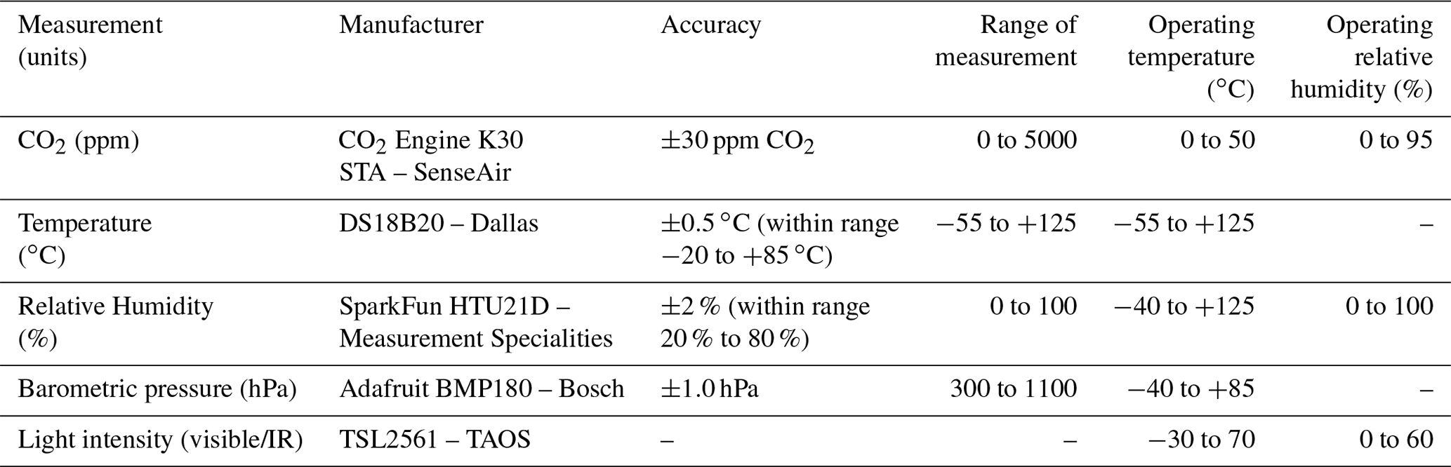
A multi-sensor portable kit, named an air enquirer (Morguí et al., 2016), was designed and built as part of an EduCaixa project (https://educaixa.org/es/home, last access: 28 April 2022). The kit consists of five low-cost sensors controlled by an Arduino Due Rev3 microcontroller board that measures the (i) NDIR CO2 concentration (in ppm), (ii) relative humidity (%), (iii) temperature (∘C); (iv) barometric pressure (hPa), and (v) light intensity (lux). Data from sensors are automatically read and stored at a frequency of 0.2 Hz on a microSD card. All sensors and the Arduino board controlling them are enclosed in a methacrylate box of cm3 in size (Fig. 1). Table 1 shows the main features of each sensor, according to the specifications provided by their respective manufacturers. The total cost of each air enquirer (AE) kit is about EUR 200.

Figure 1An air enquirer kit, with sensors for measuring temperature, humidity, barometric pressure, light intensity, and CO2 concentration in air.
Table 1Characteristics of the sensors included within the air enquirer kit.
2.2 Calibrations and multiparametric correction of the CO2 sensors of the air enquirer kit
Low-cost CO2 sensors are known to be temperature (T), humidity (H), and pressure (P) dependent (Arzoumanian et al., 2019; Martin et al., 2017). In this study, five AE kits were calibrated using different methodologies from the literature, and their responses were corrected under different climate conditions. The simultaneous use of the CO2 and the environmental parameter sensors allow for a continuous correction of the response of the CO2 sensor under different conditions of T, P, and relative humidity (RH).
First of all, a theoretical correction of the CO2 data was applied by taking the following into account: (i) the change from the ppm of CO2 in wet air to the ppm of CO2 in dry air, following Wagner and Pruß (2002) and (ii) the conversion from the ppm of CO2 measured under specific pressure to the standard pressure using the ideal gas law equation.
The concentration of CO2 in dry air (CO2_dry) was calculated by Eq. (1), as follows:
where Vdry is the volume of 1 m3 of dry air at 1013 hPa after removing the water volume. Vdry can be calculated from Eq. (2), as follows:
where Pws is the water vapour saturation. This is directly calculated from Eq. (3), as follows:
A, m, and Tn are constants with values of 6.1164, 7.5914, and 240.73, respectively.
In a second step, an experimental multiparametric calibration of the CO2 sensors was done using the data of the environmental sensors and a reference CO2 instrument. A Picarro G2301 cavity ring-down spectroscopy analyser (CRDS) was used as a second reference standard. This CRDS has a precision of better than 0.03 ppm for CO2 (Crosson, 2008; Richardson et al., 2012). The CRDS results were previously corrected for water vapour (Rella et al., 2013) and calibrated in the laboratory using six NOAA WMO-CO2-X2007 reference gases (primary standard) before and after each experiment, following Tans et al. (2011).
In order to calibrate the CO2 sensors' response for a wide range of temperature, pressure, humidity, and CO2 concentration, duplicate measurements were carried out using a temperature-controlled box at two sites, i.e. (i) at the Institut de Ciències del Clima laboratories (IC3), located at 20 m above sea level (m a.s.l.) in the city of Barcelona, Spain, and (ii) at the Centre de Recerca d'Alta Muntanya laboratories (CRAM, in the mountain town of Vielha, Spain, at 1582 m a.s.l.). Each experiment lasted 7 d and was carried out using the scheme in Fig. 2. In order to remove high-frequency variability, the sampled air was homogenised in a sealed pre-chamber prior to entering the calibration chamber. Then, the air was pumped to the calibration box at a flow rate of 0.4 L min−1 and through the secondary standard reference instrument CRDS. Both experiments were performed in a temperature range between 20 and 42 ∘C and a relative humidity with diurnal cycles between 10 % and 50 %. The temperature in the calibration box was set to be in increased in slopes of 10 ∘C, although, at low temperatures, it fluctuated with room temperature. The pressure ranged between 1004 and 1012 hPa in the calibration at IC3 and between 838 and 850 hPa in the calibration at CRAM. The two calibration experiments at the CRAM and at IC3 stations were carried out with a 1-month difference.

Figure 2System used at IC3 (Barcelona, Spain) and at the CRAM station (Vielha, Spain), for the calibration of CO2 sensors mounted on the air enquirer kits.
CO2 concentration values measured by each NDIR CO2 sensor and corrected for P and RH, using Eq. (1) (CO2 dry_kit), were calibrated by comparison with simultaneous CO2 concentration measured by the CRDS (CO2 CRDS) and considering the environmental conditions of T, absolute humidity (H), and P, using Eq. (4), as follows:
A multiparametric fit of Eq. (4) yields the following calibrated/corrected CO2 values, as reported in Eq. (5):
The CO2 corr calibrated results were compared to those obtained with a simple bias correction using the averages of CO2 CRDS and CO2 dry_kit values and also to those obtained with a simple linear calibration of the CO2 dry_kit values with the CO2 CRDS values without taking into consideration the effect of T, P, or H.
2.3 Steady-state through-flow chamber (SS-TF or open dynamic chamber)
The prototype of the open SS-TF chamber consists of two methacrylate cells of 36 L, where two AE kits are installed in each of the chambers in order to continuously monitor the CO2 concentration and environmental variables. The duplicity of the AE kits is used to ensure the reliability of the measurements. The chamber dimensions were designed to avoid border effects and minimise measurement errors, as observed by Senevirathna et al. (2007). The first chamber is a hermetic closed chamber with a unique entry for ambient air (labelled here as the mixing chamber in Fig. 3). The second one (labelled here as the flux chamber), with an open base, was installed directly over the soil.
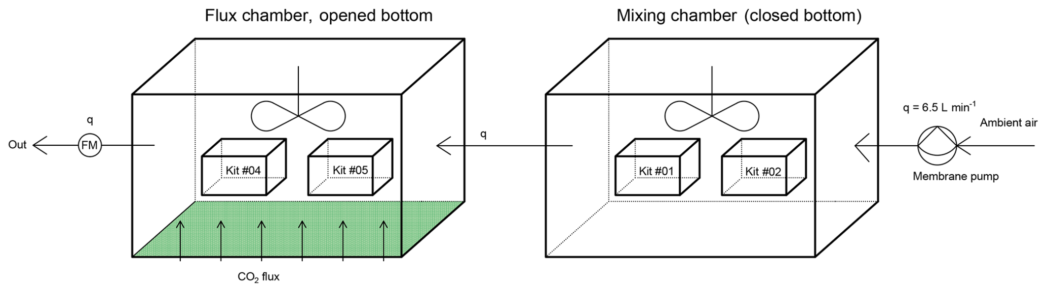
Figure 3Scheme of the dynamic SS-TF chamber designed and built at IC3 for continuous CO2 flux measurements.
The mixing chamber is used to mix the sampled air and to measure the CO2 concentration background of the atmospheric air (Cmix) before it enters the flux chamber. It contains two AE kits and a fan located at its top for mixing the sampled air. This chamber has only two openings for the inlet and outlet of atmospheric air at a flow of 6.5 L min−1 (labelled q in Fig. 3). Cable glands are used at the openings to prevent leakages. Using this configuration, a high-frequency variability in the atmospheric air could be avoided and near-steady-state conditions were reached.
The flux chamber is bottomless and has to be positioned in the first 5 cm of the soil/vegetation layer where the soil fluxes are to be measured. There were two AE kits and a vent fan installed at the top of this chamber as well. A constant flow q between the two chambers was achieved with a membrane pump and a flowmeter (labelled as FM in Fig. 3). Low flows, in comparison with the chamber volume, are needed to maintain near-steady-state conditions during measurements.
Using the system depicted in Fig. 3, CO2 fluxes ( in ) can be calculated for given time intervals within the flux chamber, using the mass balance in Eq. (6) (Gao and Yates, 1998), where V and A are, respectively, the volume of the flux chamber and the emitted soil surface area, Ca(t) (µmol L−1) is the spatially averaged concentration of the target gas in the chamber headspace, Cin(t) (µmol L−1) is the average CO2 concentration of the inlet air in the flux chamber, Cout(t) (µmol L−1) is the outflow CO2 concentration, Jg is the flux of the target gas at the enclosed soil surface, and qin and qout are the inlet and outlet flow, respectively.
Assuming that, for each measurement interval, (i) the inflow and outflow rates are constant and equal (meaning no leakages are present in the pneumatic circuit) and thus , and that the (ii) chamber reaches a steady-state condition, and thus the Cin(t)=Cin, Cout(t)=Cout, and dM(t)=0, CO2 flux can be calculated, as follows, for each time interval from the simplified Eq. (7) below:
Assuming that the fan completely mixes the air within the chamber and that the CO2 concentration at each of the boxes is homogeneous, the outflow concentration is equal to the flux chamber concentration (Cout(t)=Ca(t); as measured by the two AE kits within the flux chamber), and the inflow concentration is equal to the mixing concentration (Cin(t)=Cmix(t); as measured by the two AE kits within the mixing chamber). The advantage of this system is that fluxes can be measured continuously with a very small energy requirement (<5 W) and, even when using duplicate sensors, with a relative low cost (EUR ∼1200) in comparison with other automatic commercial flux chambers that are priced at roughly EUR 12 000. The new system described here enables the feasibility of a network of continuous measurements and a replication of experiments to cope with soil flux variability.
2.4 Non-steady-state non-through-flow chamber (NSS-NTF)
CO2 fluxes using the NSS-NTF chamber or closed static chamber are measured on the basis of the so-called linear accumulation method (Livingston and Hutchinson, 1995), which uses the initial rate of concentration increase in an isolated chamber that has been placed on the soil surface for a known period of time. Assuming ideal gas behaviour, the slope of the CO2 concentration during the accumulation interval can be used to determine the CO2 flux (), following Eq. (8) below:
where V (m3) and A (m2) are the volume of the chamber and the enclosed soil surface area, respectively, CO2_slope (ppm s−1) is the slope of the linear increment of the CO2 concentration during the early accumulation time, P and T are the atmospheric pressure and the environmental temperature within the chamber, and R (m3 Pa K−1 mol−1) is the universal gas constant. It has been pointed out that the linear approach of the accumulation method is only reliable for short time periods (Davidson et al., 2002; Grossi et al., 2012; Gutiérrez-Álvarez et al., 2020). Otherwise, the gradients of the environmental parameters between the inside and outside chamber could influence the measurement, probably yielding leakages of unknown origin in the chamber. Luckily, high-frequency measurements, such as the ones performed by CO2 sensors, allow the application of this method over a really short accumulation time (T=5 min has been used in the present study), thus complying with the theoretical requirements. A necessary condition for the application of this method is that the initial CO2 concentration within the chamber has to be equal to the atmospheric CO2 concentration. Therefore, NSS-NTF chambers need to be ventilated after each measurement period (Davidson et al., 2002; Xu et al., 2006). This can be done manually or by using automatic systems. In this study, a manual static chamber was used. A closed NSS-NTF chamber of methacrylate () cm3 was built at IC3 in order to perform a short campaign for the comparison of the CO2 fluxes measured by NSS-NTF and SS-TF systems. An AE (no. 3) and a fan were fastened at the top of the chamber. Both devices were run by a small external battery pack. An outer metallic sleeve was previously fixed onto the soil to avoid leaks and other disturbances. However, the systemic comparison between these two systems is beyond the scope of this study.
3.1 Comparison between different calibration/correction approaches
The calibration and correction factors from Eq. (5) of the CO2 sensors installed in the five AE kits are shown in Table 2. The average bias (in ppm CO2) between the AE kit CO2 value, after and before applying the theoretical corrections for P and dry air, is also shown. The last five columns of Table 2 present, for the different methodological approaches, the calculated root mean square error (RMSE), using Eq. (9), as follows:
where n is the number of values, are the CO2 values of the calibrated CRDS, and are the CO2 values of the AE sensor for each case, where kCO2 are the uncalibrated values, kCO2_dry are values corrected only for P and dry air, kCO2_dry-bias are values corrected for P and dry air, and with the average bias from the CRDS data removed, kCO2_linear are values corrected for P and dry air, and linearly calibrated with the CRDS data, and kCO2_multi are values corrected for P and dry air, and calibrated with the CRDS data using a multiparametric correction with T, RH, and P sensor data.
Table 2Parametric fitting for calibration of CO2 air enquirer sensors.
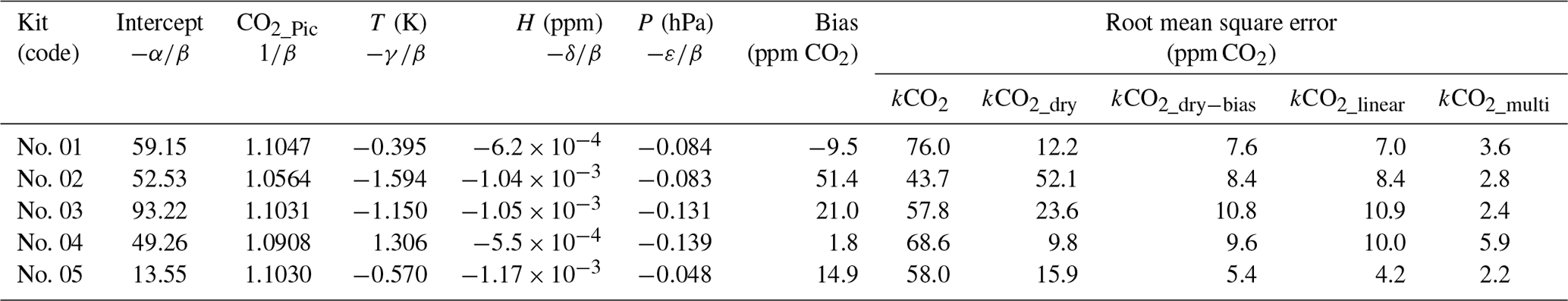
A single theoretical correction for P and RH is demonstrated that already reduces the uncertainty by a factor of 5. However, this theoretical correction is not enough for applications where the absolute CO2 value is needed (e.g. for the atmospheric composition or SS-TF measurements), as the bias value is extremely variable, depending on the sensor unit, and up to 50 ppm. When we remove the average bias between the sensor response corrected for P and RH and the CRDS CO2 reference value, the uncertainty is highly reduced, and the RMSE of the corrected values ranges between 5.4 and 10.8 ppm. This uncertainty, however, could still be too high for certain applications, such as the measurements of small atmospheric variability or for small CO2 flux measurements both for the SS-TF and NSS-NTF chambers.
Calibrating these sensors through comparison with the CRDS secondary standard in the laboratory by linear fit allows one to reach RMSEsimple values between 4.2 and 10.9 ppm. However, when the influence of the environmental parameters on the response of the sensors is also taken into account, the RMSEmulti values range is shifted to the interval between 2.19 and 5.92 ppm, i.e. the lowest ones. Figure 4 shows the time series of the differences between the CO2 CRDS data and all CO2 sensors data after applying the simple calibration (CO2_linear) and the multiparametric regression (CO2_multi). Corresponding values of T and RH measured during the calibration experiments are also reported. Each CO2 sensor responds differently to the variations in T and RH – and so do the parametric coefficients. Therefore, a theoretical correction of the CO2 value for these variables will not applicable, and a specific multiparametric fitting is needed.
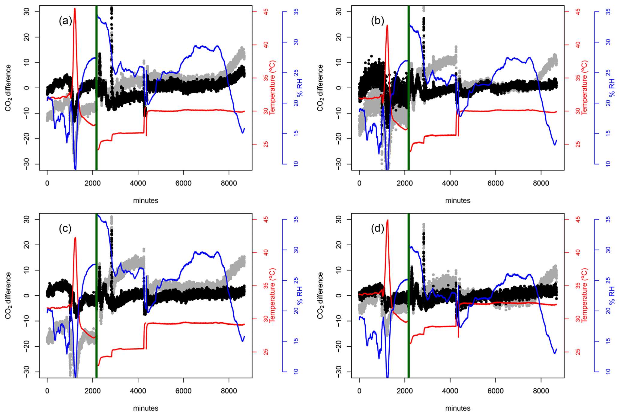
Figure 4Time series of differences between CRDS CO2 values and CO2 AE kits values after simple calibration (grey) and after multiparametric fitting (black) for AE kit no. 1 (a), kit no. 2 (b), kit no. 3 (c), and kit no. 5 (d). Temperature values (red) and RH values (blue) are also plotted. Values before the vertical green line correspond to the calibration at IC3 and after the vertical green line to the calibration at CRAM.
Figure 5 shows the relation between the reference CO2 values (CRDS) and the values measured by the CO2 sensors for raw data and after the application of the different calibration methodologies. The four sensors show RMSEmulti values lower than 5 ppm, and just one of them (kit no. 4) is greater than 5 ppm. However, this last sensor shows a negative correlation with the ambient temperature, unlike all the others, where the CO2 values increased as temperature went up. Besides, the kit was recently installed within the CO2 fluxes chamber for the second part of the study, so the results from it were not used.
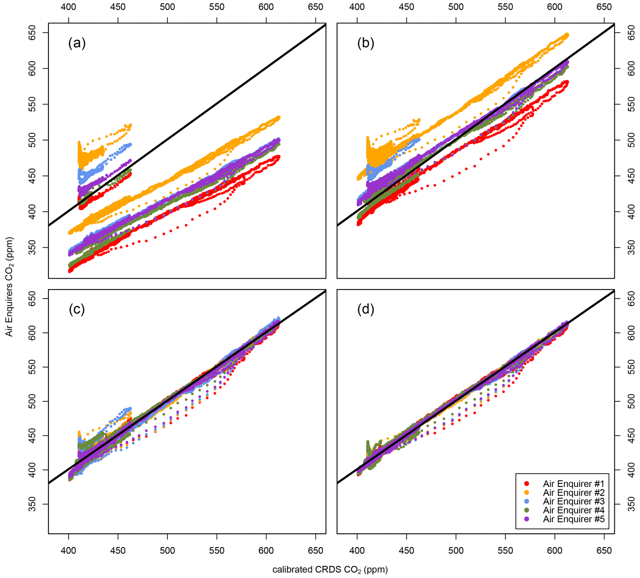
Figure 5CO2 concentrations in the air measured by each of the AE sensors during the experiment carried out at the CRAM and IC3 stations vs. CRDS data, using a sensor with raw data (a), sensor data theoretically corrected by P and RH (b), sensor data corrected by P and RH and calibrated with the CRDS (c), and sensor data corrected by P and RH and calibrated using a multiparametric lineal model (d).
A variance and covariance analysis were also performed to check the influence of meteorological parameters on the CO2 sensor response. A clear influence of temperature (T), absolute humidity (H), and pressure (P) was observed on the CO2 sensor's response (p value of for all variables). No cross-correlation was observed among variables. It is important to remark that, although the multiparametric calibration was done after applying the theoretical correction for P and RH, as explained previously, pressure conditions had the highest influence on the sensor response. In fact, a reduction of 62 % in the RMSE was observed when pressure correction was applied. Moreover, parametric values for P diverge between sensors, so every sensor seems to be differently influenced by atmospheric pressure.
3.2 Comparison between the NSS-NTF and SS-TF systems
The new prototype of the SS-TF system, described in Sect. 2.2, was briefly tested in a grassland area of the Pyrenees, near CRAM, between 1 and 2 June 2016, and compared with a manual NSS-NTF system. CO2 fluxes () were calculated for both SS-TF and NSS-NTF systems, using Eqs. (7) and (8), respectively.
CO2 concentrations from each of the sensors installed in the SS-TF chamber (upper panel) and the corresponding calculated time series (lower panel) are shown in Fig. 6. The differences between the 10 min average of the CO2 concentrations measured by the two sensors within the mixing chamber (AE kit nos. 1 and 2) were of 2.2±5.3 ppm. This difference is coherent with the RMSEmulti of both sensors and remained stable over time. The differences between the 10 min average of CO2 concentrations measured by the two sensors within the flux chamber (AE kit nos. 3 and 4) were greater (20±8 ppm) and temperature dependent, with a significant correlation (p value and r2=0.95). As the CO2 values of kit no. 4 were found to have a different behaviour during the calibration events, and the RMSEmulti was greater than 5 ppm, the values of this kit were discarded. Each value of flux was calculated using Eq. (7) and averaging the calibrated CO2 values of AE nos. 1 and 2 for the mixing chamber and using the calibrated CO2 values from AE no. 3 for the flux chamber. The 10 min averages were calculated from every minute of calculated flux data. The variability in the flux within the 10 min averages is represented in Fig. 6 as an associated uncertainty of 2σ. The associated expanded uncertainty for each value was calculated by propagating the 2×RMSEmulti of the flux chamber CO2 sensor.
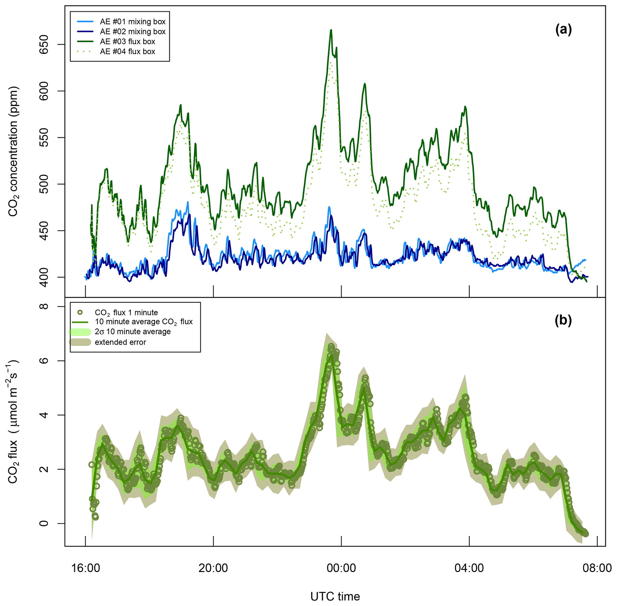
Figure 6Time series of 10 min average CO2 concentrations (a), measured within the SS-TF chamber at the CRAM grassland between 1 and 2 June 2016, and the calculated (b). The 2σ range for the 10 min average variability and the extended error (by adding 2 times the RMSE of the multiparametric fit) are also plotted.
CO2 fluxes using the NSS-NTF chamber were calculated using the slope of the increase in the CO2 concentration within the chamber and its associated uncertainty. The two examples of the CO2 concentrations measured by the CO2 sensor of kit no. 03 within the NSS-NTF chamber (see Sect. 2.3) are shown in Fig. 7. The data of the first minute after manually closing the chamber were discarded during the calculations in order to remove installation noise. Concentration gradients were linear over the following 5 min, with a correlation coefficient R2>0.99 in all cases, as calculated with Eq. (5). Positive fluxes were measured during the afternoon and negative ones in the morning, as expected, because of the photosynthesis phase of grassland plants.

Figure 7Example of two cases where the linear accumulation method was applied within an NSS-NTF chamber to calculate positive (a) and negative (b) CO2 fluxes with kit no. 3.
The correlation between both NSS-NTF and SS-TF results during the co-measurements carried out at CRAM grasslands during 1 and 2 June 2016 is shown in Fig. 8. CO2 flux values change from close to zero up to 8 . The obtained values agree with CO2 flux values observed in other studies in grasslands at a similar altitude, latitude, and period of the year, where the range of nighttime fluxes was reported to be between 2 and 4 (Bahn et al., 2008; Gilmanov et al., 2007). Although the duration of this first comparison experiment is short, the results help to strengthen the reliability of the new SS-TF chamber based on low-cost sensors. However, the size of the comparison dataset does not allow a robust statistic, and further long-term comparison should be carried out to fully characterise this new system. Indeed, the main goal of the present work is not to characterise the new SS-TF chamber but to offer a robust metrology for low-cost CO2 sensors and AE kits which can be easily applied for continuous CO2 flux measurements with high precision, low cost, and low maintenance.
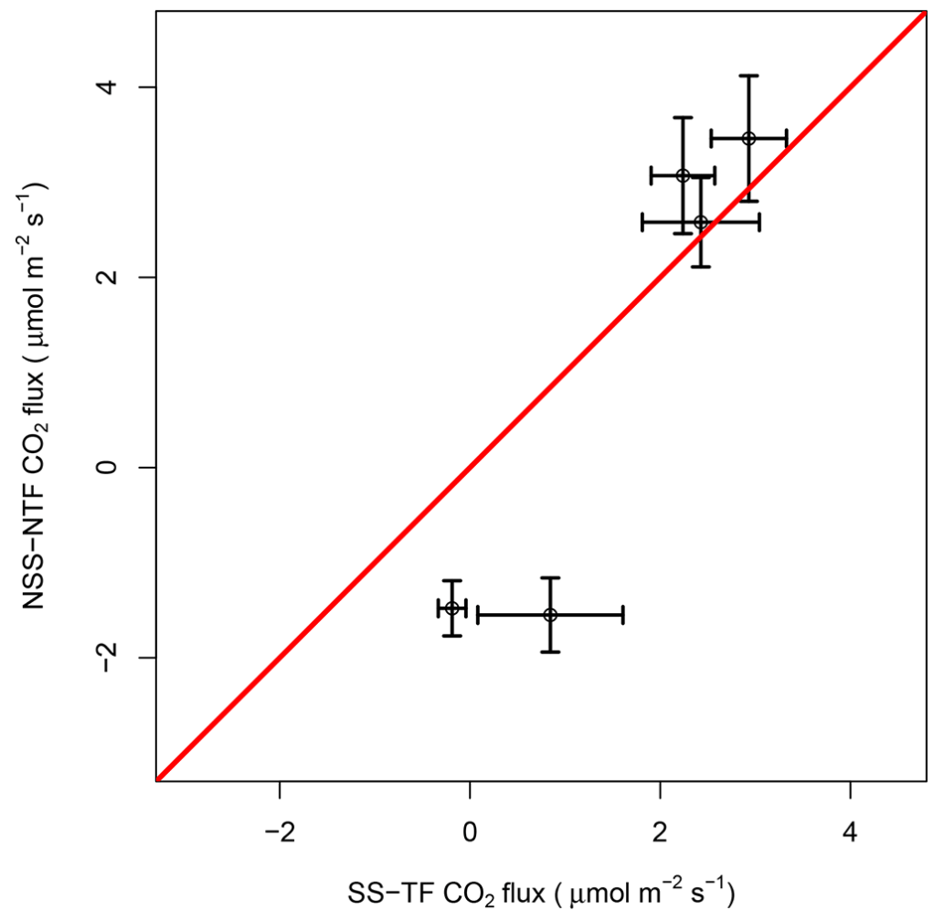
Figure 8Comparison of SS-TF and NSS-NTF CO2 fluxes during a short campaign at the CRAM station between 1 and 2 June 2016.
CO2 fluxes observations from NSS-NTF and SS-TF chambers agree for positive CO2 fluxes, while they do not for negative CO2 fluxes. A plausible cause of this mismatch may be the different degrees of opacity of the chambers, which influences the sink effect of the soil during the sunlight hours. In fact, the NSS-NTF chamber was completely translucent, while, in the SS-TF chamber, the top side was opaque.
3.3 Calibration and recalibration strategy
According to the RMSE results shown in Table 2, the multiparametric correction reduced the uncertainty of CO2 measurements by a factor of 10, compared to those where only a theoretical correction for RH and P was applied, and by a factor of 3, compared to measurements with a linear calibration only for CO2. In the SS-TF, the flux calculation depends on the difference between the absolute concentration values of the different sensors in two chambers, and a bias between them of e.g. 10 ppm will cause, in this system, a fixed bias of 0.32 in the flux calculus. Therefore, the multiparametric correction of sensors for this application is strongly recommended, together with a periodical recalibration of the CO2 sensors. Previous works with NDIR sensors have shown that it may be necessary to calibrate the sensors at least every 6 months in order to take into account possible effects due to dust and the soiling of their internal mirrors (Curcoll et al., 2019; Piedrahita et al., 2014) or the degradation of the IR light (CO2Meter.com, 2013). A mobile second reference standard could be deployed to perform an in situ calibration of the low-cost sensors. However, a periodical full calibration and calculation of correction factors for all environmental parameters could be difficult to carry out at field sites and may even cause large errors if the range of temperature, humidity, and pressure used is not large enough. For those cases where a full multiparametric recalibration could not be performed every 6 months, a bias correction should be performed at least every 6 months. This could be done by placing CO2 sensors in a mixing chamber at the same time and introducing air from a reference tank with known CO2 concentration. Thus, taking Eq. (4) into consideration, this calibration will only adjust the α parameter, considering the effects of P, T, and RH to be constant over time.
For NSS-NTF applications, where only the slope of the CO2 concentration is used, the bias has no effect on the calculus of the soil flux. Therefore, for this last case, periodical corrections for the low-cost sensors are not needed, although they are advisable to improve the quality of the measurements. Finally, when no calibrations are possible, the recommendation is to calculate the CO2 concentration in dry air and compensate for pressure. Actually, comparing NSS-NTF-based flux data, only a difference of about 4 % is observed when a theoretical correction for P and RH or multiparametric calibration data are compared. However, when using the CO2 AE kit values without any correction, this difference rises up to a 23 %.
Nowadays, the improvement in precision and cost decrease of non-dispersive infrared (NDIR) CO2 sensors have made them more readily available for multiple purposes. However, in order to apply them for atmospheric measurements where low CO2 concentrations or small CO2 variability are observed, a robust metrology is still needed to (i) ensure a traceable calibration, (ii) evaluate and correct the influence of the environmental parameters on the sensor response, and (iii) estimate the total uncertainty related with the measurements.
In this study, an analysis of the different calibration methods is carried out for NDIR low-cost CO2 sensors using air enquirer kits that are designed and built to also include environmental sensors. In addition, a new application of these sensors is presented to continuously measure the CO2 fluxes on soil with a dynamic chamber.
The lowest uncertainty for the CO2 sensors was obtained by calibrating them using a secondary standard reference (CRDS monitor) and correcting the sensors' response under different temperature, humidity, and barometric pressure conditions. A multiparametric fitting was applied to calibrate and correct the sensor's responses, achieving a drastic reduction of 90 % in the uncertainty of measured CO2 concentrations. The multiparametric calibration will ensure the highest quality of the data, and it will be advisable for SS-TF-based CO2 flux measurements or CO2 atmospheric concentrations. For NSS-NTF-based CO2 flux measurements, a correction for P and RH of the CO2 sensors will already give reliable results, although calibrating the sensors with a portable second reference standard is recommended.
The presented SS-TF chamber based on air enquirer kits allows continuous measurement of CO2 fluxes from soil and continuous ambient air CO2 concentration with low uncertainty, low cost (EUR ∼1200), low energy demand, and low maintenance. This system could be a good tool for creating CO2 flux dense networks. In the present study, it has only been shortly compared with a NSS-NTF chamber in the Pyrenees area, showing CO2 fluxes comparable between them and in agreement with the literature. However, a full characterisation of this system needs to be carried out in the future by long-term comparison with commercial CO2 flux systems.
The software code for this paper is available from the corresponding author.
The data for this paper are available from the corresponding author.
JAM coordinated the design and manufacture of the AE kits and promoted the building of the new low-cost SS-TF chamber for CO2 fluxes. LC collaborated in the mounting and tuning of the AE kits. AK, during his bachelor's degree project, participated in the laboratory and field campaigns. RC and CG performed the laboratory and field experiments, analysed the data, and coordinated the writing of the paper. AV participated in the development theoretical approach of the SS-TF methodology for gas fluxes. All authors participated in the data analysis, discussion of the results, and writing of the paper.
The contact author has declared that neither they nor their co-authors have any competing interests.
Publisher’s note: Copernicus Publications remains neutral with regard to jurisdictional claims in published maps and institutional affiliations.
The design of the AE kits and the calibration experiments of the CO2 sensors were funded by an EduCaixa grant from the CaixaBank Foundation (principal investigator, PI – Josep Anton Morguí). The open SS-TF chamber prototype was designed and build at the IC3 in the framework of the project “Methane interchange over the Iberian Peninsula” and funded by the Retos 2013 grant (grant no. CGL2013-46186-R), from the Spanish Ministry of Economy and Competitiveness (PI – Claudia Grossi).
The Authors would like to thank the Universitat de Barcelona, for the use of the CRAM facilities, and the team of the Climadat Project (CaixaBank Foundation) at IC3, for the support during the laboratory experiments.
This research has been supported by the La Caixa Foundation (grant no. EduCaixa) and by the project “Methane interchange over the Iberian Peninsula”, funded by the Retos 2013 grant (grant no. CGL2013-6186-R), from the Ministerio de Ciencia e Innovación (Spain).
This paper was edited by Reem Hannun and reviewed by Simone Baffelli and one anonymous referee.
Agustí-Panareda, A., Massart, S., Chevallier, F., Balsamo, G., Boussetta, S., Dutra, E., and Beljaars, A.: A biogenic CO2 flux adjustment scheme for the mitigation of large-scale biases in global atmospheric CO2 analyses and forecasts, Atmos. Chem. Phys., 16, 10399–10418, https://doi.org/10.5194/acp-16-10399-2016, 2016.
Arzoumanian, E., Vogel, F. R., Bastos, A., Gaynullin, B., Laurent, O., Ramonet, M., and Ciais, P.: Characterization of a commercial lower-cost medium-precision non-dispersive infrared sensor for atmospheric CO2 monitoring in urban areas, Atmos. Meas. Tech., 12, 2665–2677, https://doi.org/10.5194/amt-12-2665-2019, 2019.
Bahn, M., Rodeghiero, M., Anderson-Dunn, M., Dore, S., Gimeno, C., Drösler, M., Williams, M., Ammann, C., Berninger, F., Flechard, C., Jones, S., Balzarolo, M., Kumar, S., Newesely, C., Priwitzer, T., Raschi, A., Siegwolf, R., Susiluoto, S., Tenhunen, J., Wohlfahrt, G., and Cernusca, A.: Soil respiration in European grasslands in relation to climate and assimilate supply, Ecosystems, 11, 1352–1367, https://doi.org/10.1007/s10021-008-9198-0, 2008.
Bond-Lamberty, B. and Thomson, A.: A global database of soil respiration data, Biogeosciences, 7, 1915–1926, https://doi.org/10.5194/bg-7-1915-2010, 2010a.
Bond-Lamberty, B. and Thomson, A.: Temperature-associated increases in the global soil respiration record, Nature, 464, 579–582, https://doi.org/10.1038/nature08930, 2010b.
CO2Meter.com: AN131 – CO2 Sensor Calibration: What You Need to Know, http://www.co2meters.com/Documentation/AppNotes/AN131-Calibration.pdf (last access: 10 February 2022), 2013.
Crosson, E. R.: A cavity ring-down analyzer for measuring atmospheric levels of methane, carbon dioxide, and water vapor, Appl. Phys. B-Lasers O., 92, 403–408, https://doi.org/10.1007/s00340-008-3135-y, 2008.
Curcoll, R., Camarero, L., Bacardit, M., Àgueda, A., Grossi, C., Gacia, E., Font, A., and Morguí, J.-A.: Atmospheric Carbon Dioxide variability at Aigüestortes, Central Pyrenees, Spain, Reg. Environ. Change, 19, 313–324, https://doi.org/10.1007/s10113-018-1443-2, 2019.
Davidson, E. A., Savage, K., Verchot, L. V., and Navarro, R.: Minimizing artifacts and biases in chamber-based measurements of soil respiration, Agr. Forest Meteorol., 113, 21–37, https://doi.org/10.1016/S0168-1923(02)00100-4, 2002.
Fahlen, P., Anderson, H., and Ruud, S.: Demand Controlled Ventilating Systems Sensor Tests, Boras, Sweden, ISBN: 91-7848-331-331-X, 1992.
Gao, F. and Yates, S. R.: Simulation of enclosure-based methods for measuring gas emissions from soil to the atmosphere, J. Geophys. Res., 103, 26127–26136, https://doi.org/10.1029/98JD01345, 1998.
Gilmanov, T. G., Soussana, J. F., Aires, L., Allard, V., Ammann, C., Balzarolo, M., Barcza, Z., Bernhofer, C., Campbell, C. L., Cernusca, A., Cescatti, A., Clifton-Brown, J., Dirks, B. O. M., Dore, S., Eugster, W., Fuhrer, J., Gimeno, C., Gruenwald, T., Haszpra, L., Hensen, A., Ibrom, A., Jacobs, A. F. G., Jones, M. B., Lanigan, G., Laurila, T., Lohila, A., G.Manca, Marcolla, B., Nagy, Z., Pilegaard, K., Pinter, K., Pio, C., Raschi, A., Rogiers, N., Sanz, M. J., Stefani, P., Sutton, M., Tuba, Z., Valentini, R., Williams, M. L., and Wohlfahrt, G.: Partitioning European grassland net ecosystem CO2 exchange into gross primary productivity and ecosystem respiration using light response function analysis, Agr. Ecosyst. Environ., 121, 93–120, https://doi.org/10.1016/j.agee.2006.12.008, 2007.
Grossi, C., Arnold, D., Adame, J. A., López-Coto, I., Bolívar, J. P., De La Morena, B. A., and Vargas, A.: Atmospheric 222Rn concentration and source term at El Arenosillo 100 m meteorological tower in southwest Spain, Radiat. Meas., 47, 149–162, https://doi.org/10.1016/j.radmeas.2011.11.006, 2012.
Gutiérrez-Álvarez, I., Martín, J. E., Adame, J. A., Grossi, C., Vargas, A., and Bolívar, J. P.: Applicability of the closed-circuit accumulation chamber technique to measure radon surface exhalation rate under laboratory conditions, Radiat. Meas., 133, 106284, https://doi.org/10.1016/j.radmeas.2020.106284, 2020.
Kim, J., Shusterman, A. A., Lieschke, K. J., Newman, C., and Cohen, R. C.: The BErkeley Atmospheric CO2 Observation Network: field calibration and evaluation of low-cost air quality sensors, Atmos. Meas. Tech., 11, 1937–1946, https://doi.org/10.5194/amt-11-1937-2018, 2018.
Kunz, M., Lavric, J. V., Gerbig, C., Tans, P., Neff, D., Hummelgård, C., Martin, H., Rödjegård, H., Wrenger, B., and Heimann, M.: COCAP: a carbon dioxide analyser for small unmanned aircraft systems, Atmos. Meas. Tech., 11, 1833–1849, https://doi.org/10.5194/amt-11-1833-2018, 2018.
Livingston, G. P. and Hutchinson, G. L.: Enclosure-based measurement of trace gas exchange: applications and sources of error, in: Biogenic Trace Gases: Measuring Emissions from Soil and Water, edited by: Matson, P. A. and Harriss, R. C., Blackwell Scientific Publications, Oxford, 14–51, ISBN: 0-632-03641-9 1995.
Mahyuddin, N. and Awbi, H.: A Review of CO 2 Measurement Procedures in Ventilation Research, Int. J. Vent., 10, 353–370, https://doi.org/10.1080/14733315.2012.11683961, 2012.
Martin, C. R., Zeng, N., Karion, A., Dickerson, R. R., Ren, X., Turpie, B. N., and Weber, K. J.: Evaluation and environmental correction of ambient CO2 measurements from a low-cost NDIR sensor, Atmos. Meas. Tech., 10, 2383–2395, https://doi.org/10.5194/amt-10-2383-2017, 2017.
Morguí, J., Font, A., Cañas, L., Vázquez-garcía, E., and Gini, A.: Air Enquirer's multi-sensor boxes as a tool for High School Education and Atmospheric Research, EGU General Assembly, Vienna, Austria, 17–22 April 2016, EGU2016-17074, 2016.
Müller, M., Graf, P., Meyer, J., Pentina, A., Brunner, D., Perez-Cruz, F., Hüglin, C., and Emmenegger, L.: Integration and calibration of non-dispersive infrared (NDIR) CO2 low-cost sensors and their operation in a sensor network covering Switzerland, Atmos. Meas. Tech., 13, 3815–3834, https://doi.org/10.5194/amt-13-3815-2020, 2020.
Oertel, C., Matschullat, J., Zurba, K., Zimmermann, F., and Erasmi, S.: Greenhouse gas emissions from soils–A review, Geochemistry, 76, 327–352, https://doi.org/10.1016/j.chemer.2016.04.002, 2016.
Oliveira, L. M. L. and Rodrigues, J. J. P. C.: Wireless Sensor Networks: a Survey on Environmental Monitoring, Journal of Communications, 6, 143–151, 2011.
Piedrahita, R., Xiang, Y., Masson, N., Ortega, J., Collier, A., Jiang, Y., Li, K., Dick, R. P., Lv, Q., Hannigan, M., and Shang, L.: The next generation of low-cost personal air quality sensors for quantitative exposure monitoring, Atmos. Meas. Tech., 7, 3325–3336, https://doi.org/10.5194/amt-7-3325-2014, 2014.
Pritchard, S. G.: Soil organisms and global climate change, Plant Pathol., 60, 82–99, https://doi.org/10.1111/j.1365-3059.2010.02405.x, 2011.
Pumpanen, J., Kolari, P., Ilvesniemi, H., Minkkinen, K., Vesala, T., Niinistö, S., Lohila, A., Larmola, T., Morero, M., Pihlatie, M., Janssens, I., Yuste, J. C., Grünzweig, J. M., Reth, S., Subke, J. A., Savage, K., Kutsch, W., Østreng, G., Ziegler, W., Anthoni, P., Lindroth, A., and Hari, P.: Comparison of different chamber techniques for measuring soil CO2 efflux, Agr. Forest Meteorol., 123, 159–176, https://doi.org/10.1016/j.agrformet.2003.12.001, 2004.
Randerson, J. T., Hoffman, F. M., Thornton, P. E., Mahowald, N. M., Lindsay, K., Lee, Y. H., Nevison, C. D., Doney, S. C., Bonan, G., Stöckli, R., Covey, C., Running, S. W., and Fung, I. Y.: Systematic assessment of terrestrial biogeochemistry in coupled climate-carbon models, Glob. Change Biol., 15, 2462–2484, https://doi.org/10.1111/j.1365-2486.2009.01912.x, 2009.
Rayment, M. B.: Closed chamber systems underestimate soil CO2 efflux, Eur. J. Soil Sci., 51, 107–110, https://doi.org/10.1046/j.1365-2389.2000.00283.x, 2000.
Rella, C. W., Chen, H., Andrews, A. E., Filges, A., Gerbig, C., Hatakka, J., Karion, A., Miles, N. L., Richardson, S. J., Steinbacher, M., Sweeney, C., Wastine, B., and Zellweger, C.: High accuracy measurements of dry mole fractions of carbon dioxide and methane in humid air, Atmos. Meas. Tech., 6, 837–860, https://doi.org/10.5194/amt-6-837-2013, 2013.
Richardson, S. J., Miles, N. L., Davis, K. J., Crosson, E. R., Rella, C. W., and Andrews, A. E.: Field Testing of Cavity Ring-Down Spectroscopy Analyzers Measuring Carbon Dioxide and Water Vapor, J. Atmos. Ocean. Tech., 29, 397–406, https://doi.org/10.1175/JTECH-D-11-00063.1, 2012.
Scharlemann, J. P. W., Tanner, E. V. J., Hiederer, R., and Kapos, V.: Global soil carbon: Understanding and managing the largest terrestrial carbon pool, Carbon Manag., 5, 81–91, https://doi.org/10.4155/cmt.13.77, 2014.
Schell, M. and Inthout, D.: Demand control ventilation using CO2, ASHRAE J., 43, 18–29, 2001.
Schlesinger, W. H. and Andrews, J. A.: Soil respiration and the global carbon cycle, Biogeochemistry, 48, 7–20, https://doi.org/10.1023/A:1006247623877, 2000.
Senevirathna, D. G. M., Achari, G., and Hettiaratchi, J. P. A.: A mathematical model to estimate errors associated with closed flux chambers, Environ. Model. Assess., 12, 1–11, https://doi.org/10.1007/s10666-006-9042-x, 2007.
Song, J., Feng, Q., Wang, X., Fu, H., Jiang, W., and Chen, B.: Spatial Association and Effect Evaluation of CO2 Emission in the Chengdu-Chongqing Urban Agglomeration: Quantitative Evidence from Social Network Analysis, Sustainability, 11, 1, https://doi.org/10.3390/su11010001, 2018.
Tans, P., Zhao, C., and Kitzis, D.: The WMO Mole Fraction Scales for CO2 and other greenhouse gases, and uncertainty of the atmospheric measurements, World Meteorological Organization (WMO), GAW Report No. 194, WMO TD No. 1553, 152–159, 2011.
Wagner, W. and Pruß, A.: The IAPWS Formulation 1995 for the Thermodynamic Properties of Ordinary Water Substance for General and Scientific Use, J. Phys. Chem. Ref. Data, 31, 387–535, https://doi.org/10.1063/1.1461829, 2002.
Xu, L., Furtaw, M. D., Madsen, R. A., Garcia, R. L., Anderson, D. J., and McDermitt, D. K.: On maintaining pressure equilibrium between a soil CO2 flux chamber and the ambient air, J. Geophys. Res., 111, D08S10, https://doi.org/10.1029/2005JD006435, 2006.
Yasuda, T., Yonemura, S., and Tani, A.: Comparison of the characteristics of small commercial NDIR CO2 sensor models and development of a portable CO2 measurement device, Sensors, 12, 3641–3655, https://doi.org/10.3390/s120303641, 2012.