Improving discrimination between clouds and optically thick aerosol plumes in geostationary satellite data

Cloud masking is a key initial step in the retrieval of geophysical properties from satellite data. Despite decades of research, problems still exist of over- or underdetection of clouds. High aerosol loadings, in particular from dust storms or fires, are often classified as clouds, and vice versa. In this paper, we present a cloud mask created using machine learning for the Advanced Himawari Imager (AHI) aboard Himawari-8. In order to train the algorithm, a parallax-corrected collocated data set was created from AHI and Cloud-Aerosol Lidar with Orthogonal Polarization (CALIOP) lidar data. Artificial neural networks (ANNs) were trained on the collocated data to identify clouds in AHI scenes. The resulting neural network (NN) cloud masks are validated and compared to cloud masks produced by the Japanese Meteorological Association (JMA) and the Bureau of Meteorology (BoM) for a number of different solar and viewing geometries, surface types and air masses. Here, five case studies covering a range of challenging scenarios for cloud masks are also presented to demonstrate the performance of the masking algorithm. The NN mask shows a lower false positive rate (FPR) for an equivalent true positive rate (TPR) across all categories, with FPRs of 0.160 and 0.259 for the NN and JMA masks, respectively, and 0.363 and 0.506 for the NN and BoM masks, respectively, at equivalent TPR values. This indicates the NN mask accurately identifies 1.13 and 1.29 times as many non-cloud pixels for the equivalent hit rate when compared to the JMA and BoM masks, respectively. The NN mask was shown to be particularly effective in distinguishing thick aerosol plumes from cloud, most likely due to the inclusion of the 0.47 and 0.51 µm bands. The NN cloud mask shows an improvement over current operational cloud masks in most scenarios, and it is suggested that improvements to current operational cloud masks could be made by including the 0.47 and 0.51 µm bands. The collocated data are made available to facilitate future research.

1 Introduction

Earth-observing satellite instruments are critical for measuring geophysical parameters for weather (Eyre et al., 2019) and climate (Stengel et al., 2020). Often the first step in measuring a geophysical parameter is to determine if the scene is “clear”. This process is called cloud masking. Cloud masks are needed to observe and retrieve surface parameters. Masks are required to differentiate clouds from aerosols when running property retrievals or flux calculations. These data are integrated into climate models to generate reanalysis products such as ERA5 (Hersbach et al., 2020) as starting points for future climate modelling (Eyring et al., 2016) or for validating model outputs (Jian et al., 2020), making them an important tool in understanding the Earth's climate.

However, in many cloud-masking algorithms, high aerosol optical depth events such as dust storms and biomass burning events are also mislabelled as clouds. This may be appropriate if the aerosols would cause significant errors in the retrieval. For example, regions of high dust loadings are identified and removed so as not to bias sea surface temperature retrievals (Merchant et al., 2006). However, the application of satellite data, for example, during fire events, may be used to identify the thick aerosol plumes in order to understand the air quality. In this case, removing the thick plumes would adversely affect the intended application.

Clouds and aerosols are observed by both active satellite instruments such as Cloud-Aerosol Lidar and Infrared Pathfinder Satellite Observation (CALIPSO) (Winker et al., 2004) and passive polar orbiting satellite instruments such as the Sea and Land Surface Temperature Radiometer (SLSTR) (Coppo et al., 2013), the Advanced Very High Resolution Radiometer (AVHRR) (Stengel et al., 2020) and the Moderate Resolution Imaging Spectroradiometer (MODIS) (Justice et al., 1998). Different types of satellite instruments have advantages and disadvantages. Geostationary satellites such as Himawari-8 (Bessho et al., 2016) and the Geostationary Operational Environmental Satellite (GOES) (Schmit et al., 2005) allow for large-scale observation of atmospheric variables with high temporal resolution, medium spatial resolution and good regional coverage. However, individual passive sensors can only see in 2-D. For example, to classify whether a bright, cold pixel is snow and/or ice or a cloud top, a retrieval algorithm must be applied to the pixel to classify it. These algorithms require evaluation using ground-based instruments and active instruments to ensure that they are accurate. Active instruments, such as the Cloud-Aerosol Lidar with Orthogonal Polarization (CALIOP) lidar instrument aboard the polar-orbiting CALIPSO satellite, use on-board radiation sources to analyse the atmosphere which enables higher horizontal and vertical resolution atmospheric profiles than measurements from passive imagers; i.e. they have to ability to see vertical structure. As they have their radiation source on board, active instruments can operate independently of solar illumination and are more sensitive to thin atmospheric layers, such as thin cirrus and aerosols, than passive instruments. In addition, active sensors can retrieve the height of layers within a pixel by evaluating the strength of the return signal and time taken for the pulse to return. This makes them able to detect clouds and aerosols within their pixels much more accurately than passive instruments. However active instruments typically only have a nadir view with a small footprint, significantly reducing their spatial coverage and temporal resolution compared with passive viewing satellites. Combining the temporal and spatial resolution of passive instruments with the more accurate classification of atmospheric layers achieved by active sensors is desirable to create an optimal algorithm for classifying clouds and aerosols. By using active instruments to label passive sensor pixels, classification algorithms for passive sensors can be developed that take advantage of the increased accuracy of active sensors.

In this paper, we develop a neural network (NN) cloud mask which, while needing to perform well in all atmospheric scenarios, is specifically focused on minimising the misidentification of thick aerosol as clouds. In the following sections, we first review existing cloud-masking techniques, then we describe the approach to collocate the active and passive instruments in order to train a NN algorithm. We describe the structure of the neural network algorithm and demonstrate the algorithm performance by analysing four case studies, and comparing qualitatively and quantitatively the performance of the mask with existing cloud-masking algorithms from the Australian Bureau of Meteorology (BoM) and the Japanese Meteorological Agency (JMA) (Imai and Yoshida, 2016). The case studies and validation will present results for the cloud mask globally but the case studies will focus on distinguishing between aerosol and clouds, particularly high aerosol loading events.

2 Review of existing cloud identification techniques

Many property retrieval algorithms for passive imagers rely on empirical cloud masks to identify cloud in satellite scenes (Lyapustin et al., 2018). These masks use models of what clouds and aerosols should look like under certain conditions as tests, which are often applied in combination to satellite scenes to identify any cloud and aerosol pixels (Zhu et al., 2015; Imai and Yoshida, 2016; Le GLeau, 2016). The most significant problem with these algorithms is the dependence on a number of predefined thresholds, which leads to a high sensitivity to surface type, atmospheric variability or instrument calibration and does not capture the more complex, often non-linear relationships between instrument channels, clouds, aerosols and the surface. This can result in misidentification of thick aerosol plumes or bright surfaces as clouds or incorrectly identify thin clouds as aerosol. Products, such as Japan Aerospace Exploration Agency (JAXA)'s aerosol retrieval product and the multi-angle implementation of atmospheric correction (MAIAC) aerosol retrieval algorithm (Yoshida et al., 2018; Lyapustin et al., 2018), have cloud masks that are more suited to differentiating cloud and aerosols, although these are not perfect either. Bayesian statistical techniques can improve the speed and accuracy of classification, as well as removing the dependence on arbitrary thresholds (Uddstrom et al., 1999; Hollstein et al., 2015). However, these algorithms often struggle to capture the more complex relationships between the inputs and classifiers as they cannot fully adapt to more complex classifications, such as identifying low, cold clouds over the poles (Poulsen et al., 2020).

Machine learning techniques, such as NNs, are an alternative to conventional cloud-identification algorithms. These algorithms develop relationships between their inputs and outputs that best fit the data they are trained on, which removes any dependence on empirical thresholds and allows them to discover complex relationships between multiple input variables, potentially improving the accuracy when compared to empirical and Bayesian algorithms. Examples of neural network algorithms can be found in Sus et al. (2018), Yao et al. (2018), Mahajan and Fataniya (2019) and Poulsen et al. (2020). The disadvantage of these algorithms, at least for supervised neural nets, is that they require large amounts of accurately labelled data. This can be achieved by labelling areas as cloud or aerosol by hand as in Hughes and Kennedy (2019) and Marais et al. (2020). However, this is limited by a person's ability to accurately differentiate clouds from aerosol plumes in satellite scenes and is very time intensive. An alternative, and the method used in this paper, is to collocate the passive imagers with high-resolution vertically resolved active instruments, such as radars and lidars, to accurately label pixels which contain cloud or aerosol (Holz et al., 2008; Taylor et al., 2016). This leads to an accurate training and validation set and provides detailed information about the composition of the atmosphere within these pixels. However, the variability of cloud scenes, the narrow swath and long return-to-target times of active instruments requires a significant number satellite scenes to be processed in order to gather enough data points to effectively train a NN. Several studies have applied this technique to polar orbiting instruments, such as Poulsen et al. (2020) collocating CALIOP data with SLSTR, as well as studies by Wang et al. (2020) and Lee et al. (2021) creating machine learning algorithms for Visible Infrared Imaging Radiometer Suite (VIIRS) for cloud phase and dust detection retrieval, respectively, using data collocated with CALIOP. These studies all demonstrate the success of machine learning algorithms trained on data labelled by active instruments but do not extend the technique to geostationary instruments, which require a more sophisticated collocation technique to account for the parallax between the active and passive sensors. These studies do not focus on biomass burning plumes, which are of particular significance over Australia. In addition, in this paper, we combine this technique with explainable machine learning models to better understand the influence of passive instrument channels on the outcome of the classification.

3 Description of key data sets

Two sources of data were collocated to generate the training and validation data: the Advanced Himawari Imager (AHI) instrument aboard Himawari-8 and the CALIOP instrument aboard CALIPSO. The individual data sets are described in the following sections. The collocated data were created with the intention of identifying clouds and aerosols independently in AHI pixels using the active lidar instrument data as the truth label. While many individual data sets were collocated, not all were included in the final algorithm. The data set was split with 80 % used to train the algorithm and 20 % of the collocations used to validate the results.

3.1 Himawari-8 AHI

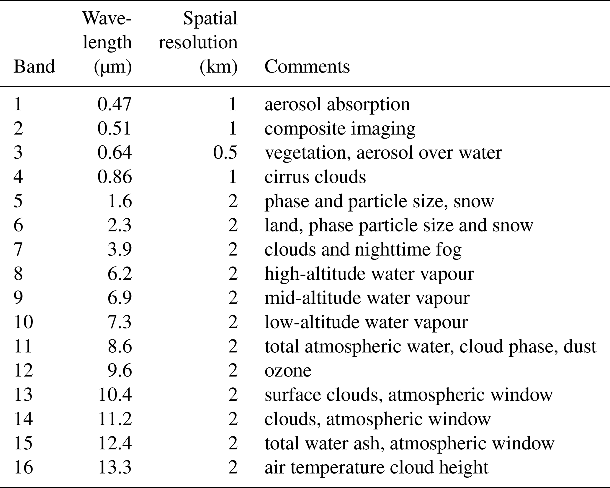
The AHI aboard the JMA's Himawari-8 geostationary satellite is a next-generation passive imager (Bessho et al., 2016). The satellite was launched in October 2014 and became operational in July 2015. AHI has 16 bands covering the visible shortwave (SW) to thermal longwave (LW) at 0.5–2 km resolutions at nadir. The channel specifications are summarised in Table 1 along with the primary objective of the channel. Full-disk scenes are centred at 140.7^∘ E on the Equator with a field of view (FOV) of approximately 80^∘ in radius and are generated every 10 min. The AHI L1b product in Himawari Standard Data (HSD) format is used for this collocation and read in using the Satpy Python package (Raspaud et al., 2021) using the default calibration. For the higher-resolution channels (see Table 1), the values are downsampled to 2 km resolution. The mean and the standard deviation of these high-resolution channels (channels 1–4) over the downsampled area are calculated and considered as inputs into the NNs. The auxiliary information from AHI is also included in the collocated data, such as the latitudes, longitudes, solar and observation angles.

Table 1 Description of Himawari-8 AHI channels (Bessho et al., 2016) and purpose (Zhang et al., 2018).

3.2 CALIOP

CALIOP is an active lidar instrument aboard NASA's polar-orbiting CALIPSO satellite (Winker et al., 2004). CALIOP uses a dual-band laser to take vertical profiles of the atmosphere directly below its orbital path every 333 m along track. This is reprocessed to 1 and 5 km along track for higher accuracy at the cost of spatial resolution. The instrument has a high sensitivity to the presence of clouds and sensitivity to particle shape and absorption characteristics, so it is able to distinguish clouds (liquid and ice) with high accuracy and between aerosol type with limited accuracy. CALIOP provides day and night global coverage, albeit with a narrow swath and long return cycle, making CALIOP useful for analysing cloud masks. Each overpass is made up of profiles containing layers with vertical resolutions dependent on the altitude of the layer that is measured by CALIOP. Measurements at both 5 and 1 km were assessed for the cloud-masking algorithm. While the 5 km algorithm is more sensitive to optically thin clouds, after initial investigation optimum results were found using the 1 km L2 cloud-layer version 4.20 product (CAL_LID_L2_01kmCLay-Standard-V4-20) (Young et al., 2018) because the higher spatial resolution leads to increased accuracy of identifying small-scale clouds in AHI pixels at 2 km resolution. The version 4 product is used for this study due to improvements made in the cloud–aerosol discrimination (CAD) score algorithm for this product (Liu et al., 2019). The CAD algorithm seeks to discriminate between cloud and aerosol particles, such as fine spherical dust particles and water clouds, by using 5-D probability density functions (PDFs) to assign values between −100 and 100 to each layer, with −100 being certainly aerosol and 100 being certainly clouds. The CAD algorithm improves on the previous version by applying the algorithm to all single-shot retrievals, which were previously classified as clouds by default, as well as making improvements to identifying elevated aerosol layers and cloud layers under dense aerosols such as smoke (Liu et al., 2019). The version 4 algorithm is validated on the 5 km product, but inspection of CAD scores between the 5 and 1 km products indicates similar performance. Therefore, although the 5 km product is more suitable for use with the CAD score, the 1 km product is still appropriate for use in this study. However, it is important to note that extreme cases of aerosols can still lead to classification of aerosol layers as cloud from the CALIOP classification and that small-scale (less then 1 km across) clouds can be potentially misclassified and be a source of error in the NNs and validation; i.e. the pixel classification by CALIOP is assumed to be true throughout this study, but CALIOP misclassifying layers is a potential source of uncertainty within this study.

The variables from CALIOP contained in the collocated data include the vertical feature mask, feature top altitudes and CAD score are saved in the collocated data file for each layer to allow for analysis of clouds and their properties.

4 Methodology

In order to create the neural network algorithms, we need to collocate AHI data with the most accurate “truth” data from the CALIOP instrument. To ensure the most applicable training data are generated, we need to take into account parallax when carrying out the collocations between the active and passive satellites. The collocated data set was then used to train and validate the neural network algorithms which are described in Sect. 4.2.

4.1 Collocation of data

The overall collocation process is shown in Fig. 1. The collocation process has two main steps. First, there is a rough collocation to identify temporally matching Himawari and CALIOP orbits and then there is a second step to perform a parallax correction.

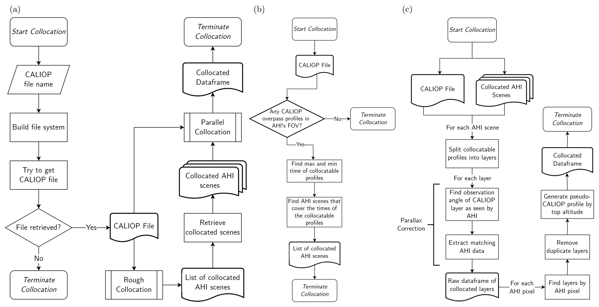
Figure 1 The full collocation process for a single CALIOP file. The full process from CALIOP file to collocated data frame is described in panel (a), whilst the processes of finding collocated AHI scenes and collocating CALIOP profile layers are described in panels (b) and (c), respectively.

The initial rough collocation, shown in Fig. 1a follows the steps below:

• The section of a full CALIOP overpass that lies within the FOV of AHI is identified; this leads to temporal uncertainty of approximately ±5 min.

• The AHI scenes that lie with the start and end of the CALIOP section run are identified.

• The AHI scenes are retrieved.

Parallax correction

Once the initial collocation is performed, the CALIOP subsection that lies within the start and end of each AHI scene scan time is found. From these sections, every CALIOP layer was parallax corrected to ensure accurate collocation with its corresponding AHI pixel. This is an important step for making sure the data set was accurately labelled. As shown in Fig. 2, the parallax between the two instruments can cause layers to be shifted by several pixels in AHI from their position as observed by CALIOP; this can be particularly significant for high clouds at the edge of the full disk. The process for performing the parallax correction is shown in Fig. 1c.

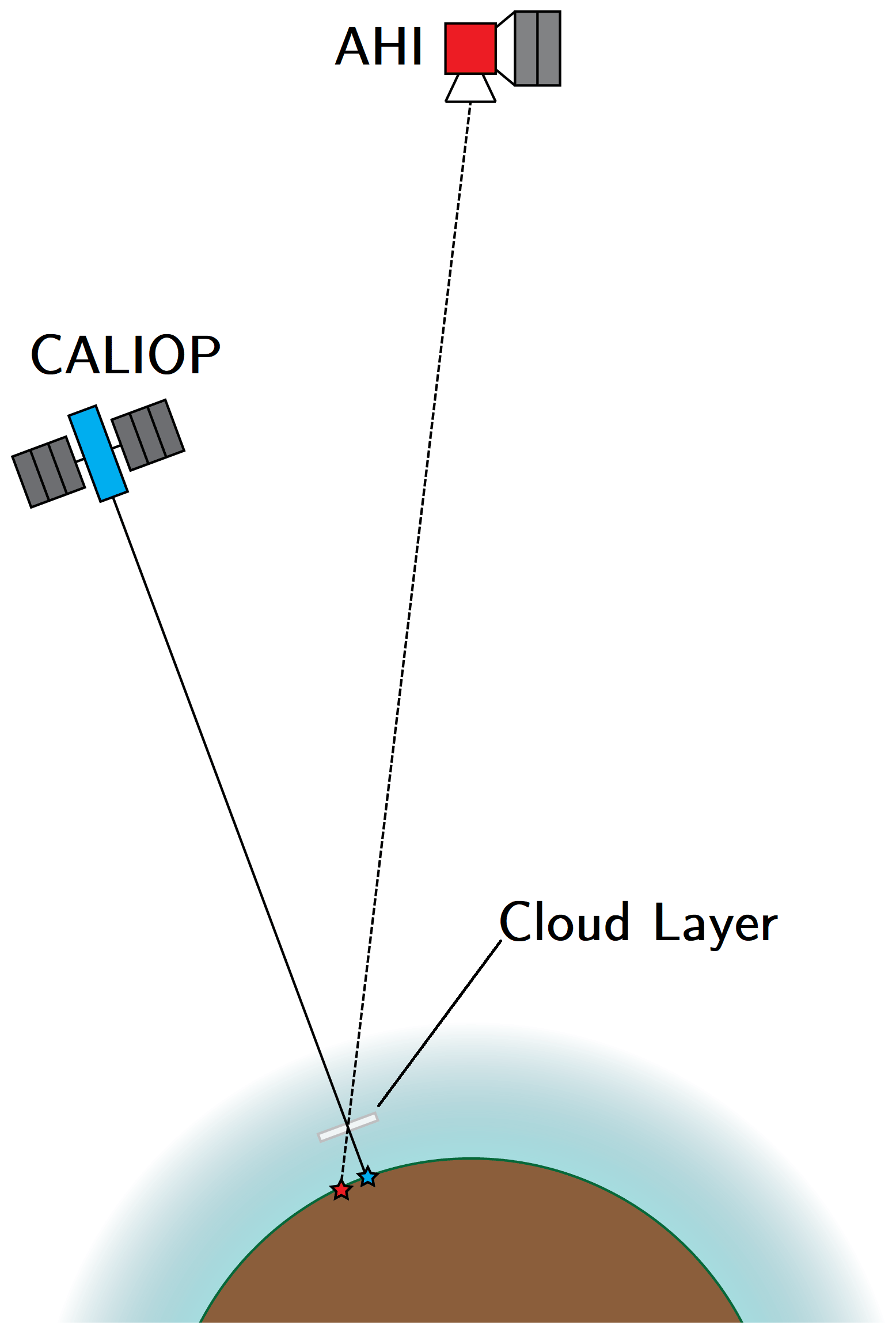
Figure 2 The difference in observation angles between CALIOP (blue) and AHI (red) for a layer (grey) at some altitude above the surface of the Earth (brown). At more extreme observation angles for AHI, i.e. towards the edge of the FOV, large differences in the apparent location of the layer can occur. For example, if the elevation angle of AHI from the layer is 45^∘ at an altitude of 10 km, the location of the layer is shifted by 10 km, approximately the equivalent of five pixels at 2 km resolution.

The parallax correction for each layer was performed by doing the following:

• The observation angles of the CALIOP layer were calculated as it would be seen by AHI at the position and altitude specified in the CALIOP data, i.e. the angle that corresponds to the dashed line beneath the cloud layer in Fig. 2.

• The observation angles of the CALIOP layer as seen by AHI were then matched with the observation angles for AHI corresponding to the Earth's surface.

• Where the AHI observation angles matched, the layer was assigned to the collocated AHI pixel; i.e. the cloud layer in Fig. 2 would be assigned to the pixel that corresponds with the red star. As the match is to the closest pixel, this leads to a spatial uncertainty of approximately ±1 km at nadir for AHI.

• This was repeated for every layer and a pseudo-CALIOP profile was generated for each AHI pixel. This includes thin layers that AHI may struggle to observe and are accepted as a potential source of error in the final cloud mask.

After each CALIOP file had been collocated, the data were cleaned by

• checking for duplicate layers and keeping only the closest matching AHI pixel and

• removing layers with AHI pixel data or CALIOP layer information missing.

These checks ensure the quality of the data in the final product is high. No further quality flags were applied to the collocated data but were instead stored with each entry to allow for further filtering of the collocated data to ensure only high-quality data were used to train the algorithm.

Approximately 7300 CALIOP overpasses were collocated for 2019 to make the full training and test validation data set, making these data suitable for large-scale statistical studies of cloud and aerosol in AHI scenes. The density distribution of collocated AHI pixels for all of 2019 is shown in Fig. 3, displaying a relatively even distribution across the AHI's field of view (FOV) for day and night. As can be seen in Fig. 3a and c, outside the polar regions, there is very little regional bias in the collocated data for day and night pixels, with the notable exception of the region where AHI's twice-daily downtime syncs with CALIOP's orbit. However, due to CALIPSO's Sun-synchronous orbit, twilight data are only available towards the poles. The concentration of collocated data at the poles for twilight scenes should be kept in mind when analysing the results.

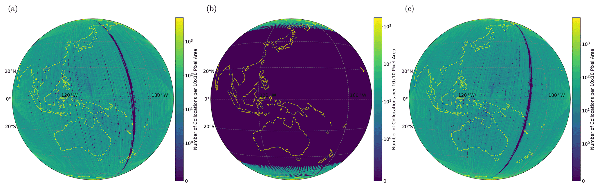
Figure 3 Heat maps of collocated AHI pixels within a 10-pixel by 10-pixel area in the AHI FOV for the full 2019 data set broken down by (a) day, (b) twilight and (c) night. The northern and southernmost region contain the highest concentration of collocated pixels as CALIOP is in a polar orbit, causing it to return to the same area in each AHI scene. Outside these regions, AHI pixels are relatively evenly distributed across the whole AHI FOV, with the exception of the region to the centre right of the FOV, which is due to AHI having gaps in coverage at 02:40 and 14:40 UTC every day.

4.2 Training and validation of neural networks

The cloud identification algorithm is based around a feed-forward neural network and implemented using the TensorFlow (version 2) package for Python (Abadi et al., 2016). Three models were created for day, twilight and night scenarios to analyse a scene pixel by pixel. The time of day was separated by solar zenith angle (SZA) and corresponding to 0^∘ ≤ SZA <80^∘, 80^∘ ≤ SZA < 90^∘ and SZA ≥ 90^∘, respectively. After experimenting with different input data, the final inputs to the neural network are as follows:

• day – channels 1–16 (mean values for downscaled channels), Himawari observation angles and cos(SZA);

• twilight – channels 1–16, including standard deviations and mean values for downscaled channels; and

• night – channels 7–16 and Himawari observation angles.

Only these inputs are used for the models. Auxiliary data, such as satellite zenith angle, latitude and longitude, are used only for further analysis of results.

For each of the different networks, the collocated data are normalised between approximately −1 and 1 to ensure optimal neural network performance using the following simple equation:

$$\begin{array}{}\text{(1)}& I_{\mathrm{norm}}={\displaystyle \frac{I-I_{\mathrm{avg}}}{I_{\max }-I_{\mathrm{avg}}}},\end{array}$$

where I is the original input value in percentage reflectance, brightness temperature and degrees for shortwave bands, longwave bands and angles, respectively, I_norm is the normalised input value, I_avg is selected by the approximate middle of the range of physically expected values, and I_max is the maximum expected input value. I_avg has values of 50, 273.15, 0 and 0 for shortwave bands in percentage reflectance, longwave bands in brightness temperature, observations angles in degrees and cos(SZA), respectively. I_max has values of 100, 423.15, 90 and 1 for shortwave bands, longwave bands, observation angles and cos(SZA), respectively. The CALIOP data are labelled using binary flags. The binary flags for cloud identification was selected from the collocated CALIOP profiles. If the top layer of the collocated CALIOP profile was found to be cloud, a filter would be applied to decide the label. If the layer has a high CAD score (CAD score > 50 Koffi et al., 2016), the layer is called a cloud layer. The CAD score filtering ensures any thick aerosol plumes from biomass burning that are occasionally flagged as clouds by CALIOP are not erroneously labelled as such for the NN training. This minimises the number of true cloud layers that are mislabelled as non-cloud in the training of the NNs. However, high thin cirrus can have low CAD scores, but the accurate labelling of elevated aerosol layers is considered to be more important for this study.

Each NN is optimised by iterating through 1, 2, 5, 10 and 20 layer structures. For each iteration, 10, 20, 50, 100 and 200 neurons were used per layer, e.g. 2 layers of 50 neurons or 5 layers of 100 neurons. All available inputs were used, and a subset of 2000 collocated data sets with a quality assurance (QA) filter of 0.7 on collocated overpasses were used for the optimisation process. This was repeated five times for the stochastic gradient descent (SGD) and Adam (Kingma and Ba, 2015) optimisers to account for different cloud and cloud-free scenarios and also to account for the statistical effect due to the small variations in the minimisation process. In total, this corresponds to 50 configurations that were investigated. The simplest NN structure with the highest average area under the receiver operating characteristic (ROC) curve value was used as the final algorithm and applied to the full data set. This is found to be 10 layers of 100 neurons each for the day, twilight and night algorithms when using the SGD optimiser. Therefore, the final structure of each NN consists of

• an input layer of N neurons, where N is the number of inputs used, with tanh activation;

• a dropout layer with dropout rate of 0.2 to prevent overfitting (Srivastava et al., 2014);

• 10 layers of 100 neurons each with tanh activation for each layer; and

• a single neuron output layer with sigmoid activation.

Each NN is trained over 200 epochs to ensure convergence. The NNs give a continuous output between 0 and 1, so an optimal threshold must be found for each NN to convert the values to a binary cloud mask. These are found after the optimisation process by taking the threshold which maximises the true positive rate (TPR) and minimises the false positive rate (FPR) of the final algorithms. For this analysis, both continuous and binary values are used.

For validation of the NNs, several metrics are used. The FPR and TPR can be calculated by applying thresholds on the continuous output of the NNs. The binary outputs can also be processed into values such as the Kuiper skill score (KSS), which is calculated by

$$\begin{array}{}\text{(2)}& \mathrm{KSS}=\mathrm{TPR}-\mathrm{FPR}={\displaystyle \frac{a}{(a+c)}}-{\displaystyle \frac{b}{(b+d)}},\end{array}$$

where a is the number of true positives, b is the number of false positives, c is the number of false negatives, and d is the number of true negatives (Hanssen and Kuipers, 1965). KSS is useful metric that balances the TPR and FPR for analysing how accurate an algorithm is at identifying cloudy pixels from non-cloudy pixels and comparing different products. A perfect KSS is 1, representing a perfect classifier algorithm, whilst 0 indicates an algorithm with no skill. Using statistical analysis alongside case studies allows for a wide-ranging analysis of the NN algorithms.

A subset of 30 collocated overpasses from 2020, which is not used in the initial training and validation, is used to carry out a statistical analysis of the NN mask, including a comparison with cloud masks from the JMA and BoM described briefly in Sect. 4.3. The masks are also compared for different case studies. These masks are chosen as they are operational cloud masks for the AHI instrument that match the NN cloud mask in spatial resolution and projection to ensure that the comparison is as fair as possible.

4.3 Description of auxiliary cloud masks

The finalised NN mask is compared to cloud masks from the BoM and JMA. The cloud masks used in the comparison are described in Sect. 4.3.1 and 4.3.2.

4.3.1 Bureau of Meteorology (BoM)

The BoM mask uses the Nowcasting Satellite Application Facility (NWCSAF) cloud-masking algorithm run with NOAA Global Forecast System (GFS) (NOAA, 2021) numerical weather prediction (NWP) information. The full description of the algorithm is given in Le GLeau (2016) and the key features are outlined below.

• The algorithm is based on look-up tables (LUTs) to calculate thresholds which are applied to individual pixels to identify cloud.

• The algorithm is split into land and sea algorithms for an initial run. These algorithms use a combination of thermal channel differences during day, twilight and night, as well as the 0.6 µm channel during day and twilight.

• A range of other threshold tests are applied to further identify features which are usually difficult to identify, e.g. low-level clouds, cloud edges, thin cirrus.

4.3.2 Japanese Meteorological Agency (JMA)

The JMA mask is based on both the NWCSAF Cloud Mask (CMA) (Le GLeau, 2016) and NOAA Advanced Baseline Imager Clear Sky Mask (ACM) products (Heidinger and III, 2013). The full algorithm description can be found in Imai and Yoshida (2016).

• The main concept behind the JMA cloud mask is to compare AHI channel data to NWP values to decide if a pixel is cloudy.

• A subset of nine channels is used (bands 3, 4, 5, 7, 10, 11, 13, 14 and 15).

• Snow and/or sea ice are filtered and flagged ice are filtered and flagged in final cloud mask.

• Aerosol pixels are also filtered using the ash detection algorithm from Pavolonis et al. (2013).

• The cloud mask utilises information from the previous scene and a scene 1 h prior to capture temporal variation.

5 Results

5.1 Statistical comparison of cloud masks using CALIOP

The cloud masks were compared statistically by using collocated CALIOP data as the truth label. There are 30 collocated data sets, where each data set is a CALIOP overpass that has been collocated with AHI data, that were not used for training and validation were analysed by the NNs. This data set consisted of approximately 60 000 collocated pixels randomly selected from January to June 2020. The pixels were also collocated with the matching BoM and JMA binary cloud masks. An example of collocated data used in this comparison is shown in Fig. 4 with the cloud masks and truth label shown above the profile curtain plot to demonstrate the strengths and weaknesses of each cloud mask. It can be seen that the NN and JMA cloud masks show similar performance, whilst the BoM mask classifies most pixels on either side of clouds as clouds, leading to a conservative cloud mask. This performance is further demonstrated in the statistical analysis.

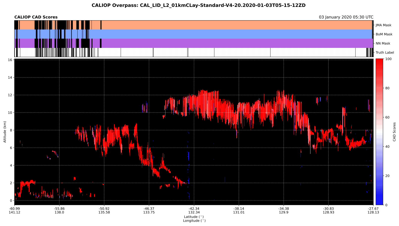
Figure 4 The CAD scores from a collocated CALIOP overpass are plotted along with the cloud masks used in this study and the truth label used for training the NN algorithms.

The TPR and FPR for each cloud mask was calculated and plotted on a ROC curve representing the combined outputs of the NNs in Fig. 5. An overall comparison of the performance shows that the NN cloud mask has the best performance over all, with a KSS of 0.632 versus 0.523 for the JMA product and 0.432 for the BoM product. The low FPR and low KSS of the JMA product suggest a cloud mask that balances cloud masking without being conservative, i.e. classifying non-cloud pixels as cloud to ensure all clouds are cleared in a scene, but does not perform as well as the NN, whilst the high FPR and low KSS of the BoM mask suggests a cloud mask that overclassifies pixels as cloud. The combination of high TPR and high KSS shows that the NN is better at not classifying non-cloudy pixels as cloudy than the JMA and BoM masks. This is important for accurately identifying optically thick aerosol plumes.

The continuous output of the NN mask can have any threshold applied to produce a binary mask; e.g. all pixels with continuous values greater than 0.5 can be assigned as clouds. The values presented were found after optimisation, but the threshold can be adjusted so that it matches the TPR or the FPR of the other algorithms. In this analysis, the threshold that yields the equivalent TPR of the BoM and JMA algorithms separately was calculated and are represented by the dashed coloured lines in Fig. 5. The blue and magenta horizontal lines correspond to the TPRs of the BoM and JMA masks, respectively, whilst the same coloured vertical lines show the FPRs of the NN mask at those TPRs. If the NN thresholds were chosen so that the TPR of each algorithm matched, the associated FPRs would be 0.363 versus 0.506 for NN and BoM algorithms and 0.160 versus 0.259 for the NN and JMA algorithms, respectively. This implies that the NN accurately identifies 1.13 and 1.29 times as many non-cloudy pixels when compared to the BoM and JMA masks, respectively, if the binary output threshold is tailored to match their TPRs.

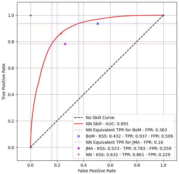
Figure 5 ROC curve comparing the false positive and true positive rate of the cloud masks. The ROC curve is produced using the continuous output from the neural network, whilst each point is calculated using the binary cloud mask for each algorithm. The dotted lines indicate where the algorithm point would be if it used a binary threshold that matched the associated algorithms' (denoted by colour) TPR.

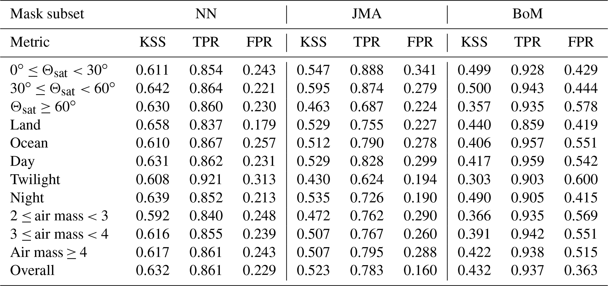
The performance for each mask was further broken down by satellite zenith angle, solar zenith angle, air mass and surface type (over ocean or over land). The results show that the NN algorithms perform best during day and night but have lower performance during twilight, where the FPR increases significantly over the day and night algorithms. Overall, the NN mask shows a notable improvement over the BoM and JMA masks, which show lower values of KSS for all situations. From the TPR and FPR values presented in Table 2, the JMA mask generally has similar TPR values when compared to the NN in all scenarios but with higher FPR values, whereas the BoM mask has significantly higher TPR and FPR values. This shows that the JMA and BoM masks are more conservative than the NNs; i.e. the NNs are better at accurately identifying non-cloud during all conditions. The NN mask also outperforms the other masks at all satellite zenith angles, retaining similar TPR and FPR values over all angles and does not drop in performance towards the edge of the scene at the same rate as the BoM and JMA masks. In particular, the BoM FPR values increase significantly with satellite zenith angle, leading to very poor performance at high angles. All the algorithms show approximately equivalent changes in performance for air mass values above 3, but the NN mask does not have as large a drop-off at low air mass values.

Table 2 Summary of KSS, TPR and FPR for various angular geometries, surface types and air masses. Note that Θ_sat is the satellite zenith angle.

5.2 Explainable machine learning

Machine learning models are often seen to be opaque black boxes from which it is difficult to extract physical interpretations. However, there exists new tools that can begin to explain the performance of individual machine learning models. SHAP (Lundberg et al., 2020; Lundberg and Lee, 2017) is one such tool. The package is based on the Shapley game theory approach to explain multi-input models. SHAP works by perturbing each model input over several iterations and calculating how much this affects the final output of the model. From this, a value related to the importance of the input can be extracted for the model. Carrying out this analysis for a range of pixels, both cloud and non-cloud, allows the otherwise opaque models to be analysed statistically. In addition using this tool, it is possible to identify the importance of each input for an individual pixel.

The final versions of the day, twilight and night NNs that make up the NN cloud mask are analysed using the SHAP package. As the SHAP computation is computationally expensive, the results of averaging five different subsets of 200 randomly sampled pixels per iteration for each NN over land and ocean are presented in Fig. 6. The error bars are generated by taking the standard deviation from the sample of five subsets.

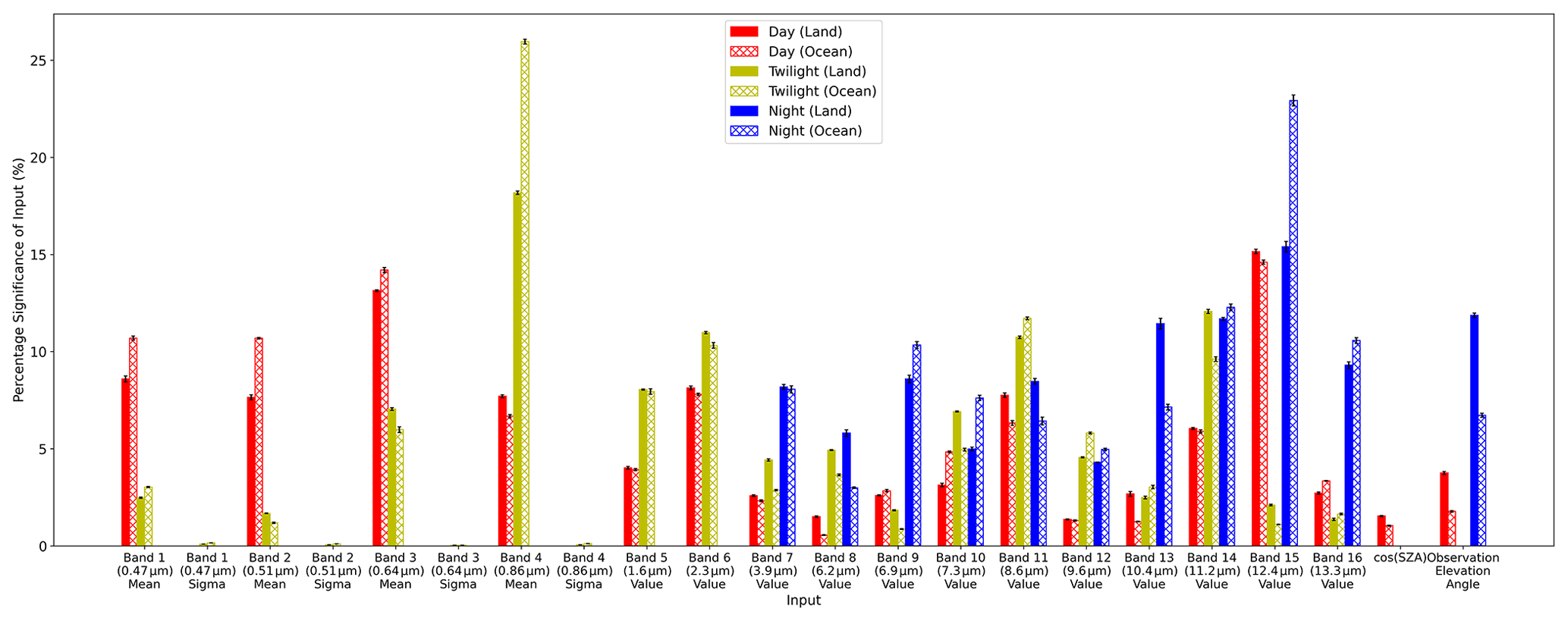
Figure 6 Plot summarising the output from the SHAP analysis. The SHAP values for each scenario, day, night, twilight, sea and land are normalised to 100. The results indicate the relative contribution of each input to defining the cloud mask.

These results show that during the day, for both land and ocean, the NN relies on information found in the visible and near-visible shortwave infrared (SWIR) mean values, as well as channels in the longwave infrared (LWIR), with band 15 (12.4 µm) being particularly important due to a small amount of water vapour absorption compared with the “cleaner” band 13 (10.4 µm) channel. The high importance of the SW channels is due to the spectral response of clouds in the visible and SWIR bands, which differs compared to most surface types, especially over the dark ocean surface. From Fig. 6, the relatively high significance values for the visible channels show that they are particularly important over land, where it can be seen that the blue (0.47 µm) band – band 1 – is approximately as important as band 2 (0.51 µm) and almost as important as band 3 (0.64 µm). Furthermore, the different spectral responses of cloud and aerosol in the blue band are likely why the NN shows a notable improvement over the other algorithms, especially during high aerosol loading events as those that will be shown in Sect. 5.3. Bands 1 and 2 are not used in the JMA and BoM cloud masks, so that may be one of the key reasons for the improved performance of the NN algorithm. The dependence on LWIR atmospheric windows is due to the difference in brightness temperature between the surface and cloud, particularly at higher altitudes. In addition, the relatively high importance of band 11 (8.6 µm), which contains information on cloud phase (see Table 1), suggests the NN is attempting to extract information on the microphysical properties of a pixel from this band and may be a key factor in the improvement of the NN dealing with optically thick aerosol plumes when used in combination with the visible bands. The relatively high dependence on the observation angle implies that the NN is accounting for aberration and path-length effects on the spectral response of clouds at the edge of a scene. The solar zenith angle during day and other water vapour channels were not found to be important.

For night pixels, it can be seen that band 15, the thermal window channel at 12.4 µm, dominates the classification skill over ocean, whilst the importance of all the channels is much more evenly distributed for land pixels. Band 15 is important for detecting low-level moisture and can be useful in identifying low-level cloud that might be of a similar temperature to the sea surface temperatures in other channels, leading to the high importance over ocean. Over land, the larger range in surface temperature values at night leads the NN to depend on several inputs rather than a single atmospheric window channel. The relatively high importance of band 7 (3.9 µm), which has a SWIR and LWIR component, suggests the NN is also extracting information on low-level cloud from this band. Observation angles are also important for the night algorithm likely due to the path length of radiation in the atmosphere, as well as potentially being used as a proxy for identifying high-latitude regions.

Twilight pixels are a challenge for cloud masks due to the very high air mass values causing visible channels to appear significantly different from the day equivalents. The twilight NN appears to place lower importance on the shorter wavelength visible channels, which are more strongly scattered during twilight, and instead relies more strongly on the band 4 (0.86 µm) mean, the SWIR and the thermal channels. Over ocean, the NN places very high significance on the band 4 mean, which is less affected by Rayleigh scattering and is dark for the ocean surface. This suggests the algorithm looks for high band 4 values to identify cloud over ocean in combination with the traditional infrared window channel of band 14. Over land, bands 11 and 14 have approximately equivalent significance in the NN. Bands 4 and 14 serve the same role over land as they do over ocean. However, unlike over ocean, some land surface types can be bright in band 4 at twilight. This causes the NN to require an additional cloud-detection band to effectively identify cloud over land during twilight, and the NN has found band 11 to be most useful for this purpose.

5.3 Case studies

In this section, we present a full-disk comparison, a case study over China during a significant dust storm and three regional case studies over Australia.

5.3.1 Full disk: global view

The case study presented in Fig. 7 is a full-disk scene for 1 November 2020 at 03:30 UTC. The scene is predominantly daylight, with twilight just appearing in the top right of the image. A region of sunglint can be seen north of Australia.

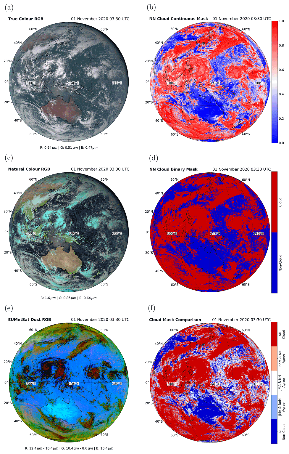
Figure 7 A full-disk AHI scene for 1 November 2020 at 03:30 UTC. A total of three RGB false-colour composites of the scene are presented in the left-hand column, showing (a) true-colour, (c) natural-colour and (e) dust RGBs. The top, middle and bottom panels of the right-hand column show (b) the NN continuous cloud mask, (d) NN binary cloud mask and (f) a comparison of the three binary masks for the scene.

All the case studies have the same format, with Fig. 7a, c and e showing true-colour, natural-colour and EUMETSAT-style dust RGB false-colour composites. The true-colour RGB false-colour composite is generated from the visible bands (bands 1–3) to show approximately how the scene appears if observed with the human eye. The natural-colour RGB false-colour composite uses bands 2–4 and shows vegetated areas as green, arid areas as pale brown, cold ice-phase clouds as pale blue and warmer water-phase clouds as white. Both the true and natural-colour RGB false-colour composites show sunglint due to the presence of shortwave bands. The EUMETSAT-style dust RGB false-colour composite is derived from bands 11, 13 and 15 and does not show any sunglint due to being purely thermal channels. This RGB false-colour composite can be used at night and is particularly useful as it shows cold clouds as black and red, including thin cirrus, and shows thick dust plumes as purple. In Fig. 7b, d and f, results from the cloud masks are shown. In Fig. 7b, the continuous output from the NN mask is shown for the scene. In Fig. 7d, the binary cloud mask from the NN is shown. Finally, in Fig. 7f, a comparison between the NN, BoM and JMA masks is shown. In this comparison, dark red and dark blue correspond to where all masks agree there are clouds and non-clouds, respectively. The pale red sections are where the BoM and NN masks agree, but the JMA mask gives a different classification; e.g. BoM and NN indicate clouds but JMA indicates non-clouds. Similarly, white is where JMA and the NN agree and pale blue is where JMA and the BoM masks agree. From the NN binary mask and the mask comparison, the class assigned by the JMA and BoM masks can be inferred.

Three different RGB false-colour composites are presented which highlight different features in the scene, such as ice-phase clouds which appear cyan in the natural-colour RGB false-colour composite. Both the continuous output from the NN algorithm and the binary mask are shown in Fig. 7b and d and show that regions of small clouds and cloud edges are the most uncertain for the NN mask. Figure 7f shows the comparison between the NN, BoM and JMA cloud masks. All three masks show good agreement for the majority of pixels, with areas of high cold clouds shown as red and clear land and ocean broadly shown as blue. Generally, areas where cloud masking appears to fail are towards the edges of clouds and clouds at small scales. At approximately 10^∘ S, towards the centre of the scene, there is a small region of sunglint. Some very small areas within this region, concentrated just north of Australia, are shown as pale blue in the mask comparison, indicating that the JMA and BoM cloud masks agree on the classification of this region but the NN mask disagrees with the other masks. In the NN mask, it can be seen that the area of sunglint is broadly shown to be non-clouds; i.e. the mask is not misclassifying some sunglint pixels, whilst the BoM and JMA masks are. In the twilight region of the scene, which is outside the collocated region of twilight data, it can be seen that the NN cloud mask fails to detect low-level clouds. This is likely due to low-level clouds outside the collocated region appearing significantly different to those within the region. The NN mask likely interprets the cool bright surface as polar surface and such behaviour is expected when using an algorithm significantly beyond its training data set. Therefore, the twilight algorithm does not perform well outside the region it was trained on, and aiming to improve this algorithm will be an area of future development.

5.3.2 Dust storm over China

The scene presented in Fig. 8 shows a significant dust storm over China from 15 March 2021 at 03:30 UTC. In Fig. 8e, the dust plume can be seen as the pink region across China towards the north of the centre of the scene and is partially covered by clouds. In addition, there is a region of snow and ice towards the north of the scene which is also covered by some clouds. From Fig. 8d and f, it can be seen that the NN cloud mask improves on the JMA and BoM masks when dealing with snow and ice in the north of the scene as it does not misclassify the majority of the snow and ice. The JMA and BoM masks fail to effectively classify the dust plume, which the NN mask accurately identifies as non-clouds. Given that this event was a historically significant event with an unusually high plume (Filonchyk, 2022), the failure of the cloud masks might be expected. However, large areas of the dust plume are assigned relatively high values by the NN mask. In Fig. 8b, it can be seen that the section of the dust plume that is towards the centre of the scene is assigned scores slightly below those assigned to clouds – the plume has values of approximately 0.5, whereas clouds have values close to 1 – indicating that, although the NN mask is not confident the plume is clouds, the dust storm poses a challenge to the NN mask classification algorithm. A future algorithm could use this information within convolutional NNs to improve the performance further for large plumes or to develop uncertainty metrics.

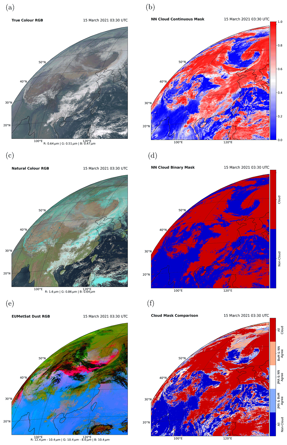
Figure 8 A partial-disk AHI scene covering southeast Asia for 15 March 2021 at 03:30 UTC. A total of three RGB false-colour composites of the scene are presented in the left-hand column, showing (a) true-colour, (c) natural-colour and (e) dust RGBs. The top, middle and bottom panels of the right-hand column show (b) the NN continuous cloud mask, (d) NN binary cloud mask and (f) a comparison of the three binary masks for the scene.

The following case studies look at a mixture of high aerosol optical depth (AOD) events, small and subpixel clouds and sunglint in scenes from Australia. The regions each of the case studies cover are shown in Fig. 9a and b.

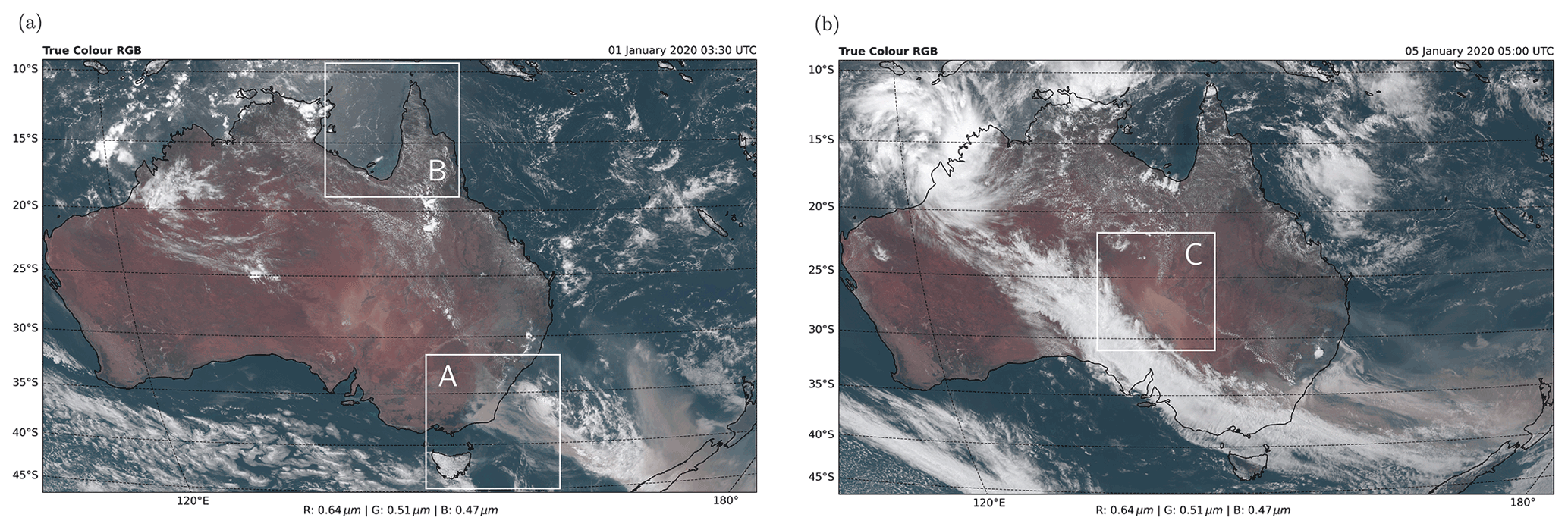
Figure 9 True-colour RGB false-colour composites from AHI scenes over Australia for (a) 1 January 2020 at 03:30 UTC and (b) 5 January 2020 at 05:00 UTC showing the approximate areas of three case study regions. Region A contains an optically thick smoke plume on the SE coast of Australia, whilst region B contains a challenging scenario for cloud masks in the Gulf of Carpentaria. Region C contains a thick dust plume in central Australia.

5.3.3 Australian case study A: smoke from the 2019–2020 Australian bushfires

Case study A is a region on the southeast coast of Australia from an AHI scene on 1 January 2020 at 03:30 UTC during the “Black Summer” bushfires (see Fig. 10). This scene shows an optically thick smoke plume as well as thick and optically thin clouds. This scene shows the difficulty in distinguishing between smoke and clouds. The majority of the smoke plume is successfully classified as non-clouds by the network. When compared to the other cloud masks, it can be seen that the network classifies less of the smoke as clouds than the JMA mask and both classify significantly less smoke as clouds than the BoM mask, which classifies optically thin smoke as clouds. There are regions off the coast towards the centre of the scene that are classified as clouds by the NN and appear to be low, warm clouds under optically thick smoke. This is not surprising as the spectral signature is predominantly sensitive to the top layers of aerosol or clouds.

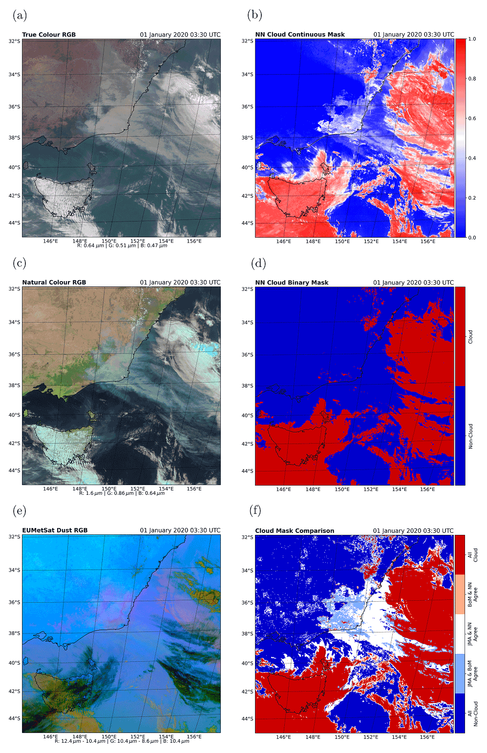
Figure 10 Region A on the SE coast of Australia from an AHI scene for 1 January 2020 at 03:30 UTC. A total of three RGB false-colour composites of the scene are presented in the left-hand column, showing (a) true-colour, (c) natural-colour and (e) dust RGBs. The top, middle and bottom panels of the right-hand column show (b) the NN continuous cloud mask, (d) NN binary cloud mask and (f) a comparison of the three binary masks for the scene.

The overall improvement in performance for the NN mask is likely due to including the additional channels not included in the JMA or BoM masks. In particular for distinguishing optically thick smoke during the day, we expect the 0.47 µm channel to add useful information, as the spectral response of cloud and smoke are significantly different in this band (Gautam et al., 2016). However, there are small regions of the smoke plume over land and along the coast which are classified erroneously as clouds by the NN. From the continuous mask, it can be seen that these regions are classified as cloud by the NN mask with relatively high confidence. Parts of these regions correspond to clouds which can be seen in the natural-colour RGB false-colour composite but not all of it. Comparing the areas that do not appear to have clouds with the dust RGB false-colour composite show that it aligns approximately with regions of dense smoke that have a pink colour, suggesting that the smoke plume has significant dust contamination. In addition, these regions may contain particularly high levels of water vapour, which from Sect. 5.2 is known to be important in cloud classification for the NN. This water vapour likely comes from the intense period of fire activity from just before this case study (Peterson et al., 2021). There is the possibility that the water vapour has begun to condense within these regions of the plume and therefore could be forming cloud particles. However, without the ability to eliminate the presence of cloud beneath this layer, it is not possible to determine the exact cause of this issue and further investigation is warranted.

5.3.4 Australian case study B: northern Australian mixed scene

This case study is also taken from 1 January 2020 at 03:30 UTC and covers the Gulf of Carpentaria and northern Queensland (see Fig. 11). The region illustrates many scenarios that are typically difficult to identify with cloud masks. Present in this scene is sunglint in the top left, sediment in the water off the coast, thin cirrus at the top of the scene and subpixel clouds over the land.

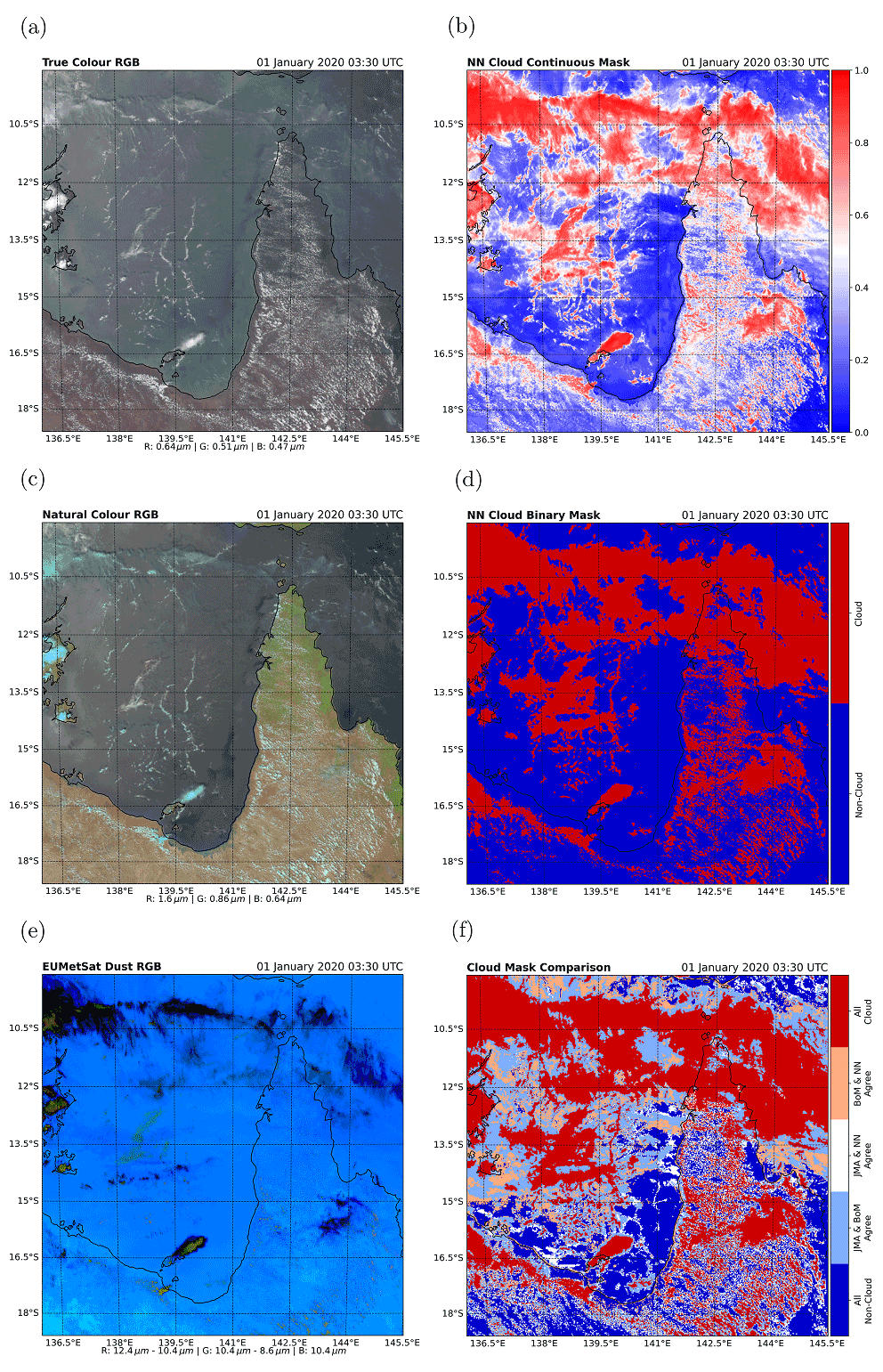
Figure 11 Case study B covering the Gulf of Carpentaria from an AHI scene for 1 January 2020 at 03:30 UTC. A total of three RGB false-colour composites of the scene are presented in the left-hand column, showing (a) true-colour, (c) natural-colour and (e) dust RGBs. The top, middle and bottom panels of the right-hand column show (b) the NN continuous cloud mask, (d) NN binary cloud mask and (f) a comparison of the three binary masks for the scene.

In this region, high, cold ice-phase clouds are consistently flagged as clouds by all the masks. However, both the JMA and BoM masks falsely classify more non-cloud pixels as clouds than the NN mask does over ocean. Towards the left of the scene, the JMA and BoM masks misidentify areas of sunglint as clouds. Both the JMA and BoM masks also identify the edges of areas of murky water off the west coast of Cape York as clouds. Over land, the low, warm, small-scale clouds over Cape York are not well identified by the NN, whereas the JMA and BoM masks flag more of this areas as clouds.

5.3.5 Case study C: central Australian optically thick dust

Figure 12 shows a region in central Australia with a thick dust plume from 5 January 2020 at 05:00 UTC. This plume is accurately classified by the NN, and the majority of the plume is correctly classified by the BoM mask. However, both the BoM and JMA misclassify some or all of the plume as clouds. To the north of the dust plume, there is a salt lake visible in the image. This is classified by the NN as non-clouds but misclassified by the other masks. This indicates another area of improvement for the NN and is particularly important for retrievals over Australia where salt lakes are prevalent.

Figure 12 Region C covering central Australia and highlighting a dust storm for 5 January 2020 at 05:00 UTC. A total of three RGB false-colour composites of the scene are presented in the left-hand column, showing (a) true-colour, (c) natural-colour and (e) dust RGBs. The top, middle and bottom panels of the right-hand column show (b) the NN continuous cloud mask, (d) NN binary cloud mask and (f) a comparison of the three binary masks for the scene.

Towards the centre and top of the scene there are areas of small-scale clouds. The JMA and BoM masks identify the majority of the cloud in this region, whereas the binary NN mask fails to identify the smallest clouds. However, it can be seen that this region has values of approximately 0.5 or higher in the continuous mask, indicating that a lower threshold could lead to better classification. The dust plume has continuous values significantly below 0.5, so decreasing the threshold would not lead to misclassification of the dust plume, allowing the NN to be significantly more accurate than the other masks in this scenario.

6 Conclusions

Identifying cloud-affected scenes in satellite data is an important step prior to retrieving geophysical properties from remote sensing data. Failure to identify clouds correctly can result in substantial biases in a geophysical retrieval. In practice, this means that cloud masks are tailored towards conservatively clearing any non-surface features at the cost of identifying many non-cloud scenes as clouds.

However, conservative cloud masks can introduce other biases. In the cases of air quality and fire applications, it is important to remove clouds while still identifying the thick aerosol plumes. In this study, a set of neural networks (NNs) are developed to improve the detection of clouds and aerosol for AHI (Bessho et al., 2016) scenes with the specific goal of identifying cloud-affected scenes as accurately as possible and at the same time improving cloud–aerosol discrimination during heavy aerosol loading events.

Data for training and validating these NNs are generated by collocating the AHI instrument with parallax-corrected CALIOP (Winker et al., 2004) 1 km cloud-layer products. Approximately 7300 CALIOP overpasses are collocated from 2019 for training separate day, twilight and night algorithms. These algorithms are optimised by sweeping over a range of possible structures using either the stochastic gradient descent or Adam optimisers. The optimal algorithms are then statistically compared to the Japanese Meteorological Agency (JMA) and Bureau of Meteorology (BoM) operational cloud masks (Le GLeau, 2016; Imai and Yoshida, 2016; Heidinger and III, 2013) using 30 collocated CALIOP overpasses from 2020. Analysis of KSS values showed that the NN cloud mask is an overall improvement over the BoM and JMA cloud masks in all scenarios. When using the NN with a true positive rate equivalent to the other masks, the NN accurately detects 1.13 and 1.29 times as many non-cloud pixels versus the JMA and BoM masks, respectively.

The NN algorithms were analysed using the SHAP package (Lundberg et al., 2020; Lundberg and Lee, 2017) to understand the influence of each input on the NN performance. For the day algorithm, it is found that all the visible channels are important, including bands 1 (0.47 µm) and 2 (0.51 µm), as well as the atmospheric window thermal channels. The night NN relies on the atmospheric window channels, as well as band 7 (3.9 µm), whilst the twilight NN relies heavily on the band 4 (0.86 µm), likely due to less Rayleigh scattering in these bands compared with shorter wavelengths, as well as the SWIR channels values to classify clouds, and the traditional atmospheric window thermal channel. However, a lack of collocated twilight data outside the polar regions limits the finding for twilight scenes.

The masks were compared for several AHI scenes covering a range of difficult scenarios, the results suggested the NN mask improves on the JMA and BoM masks for optically thick aerosol plumes, regions of sunglint and challenging surface types. One case study was a scene that contained a very optically thick smoke plume, taken from 1 January 2020 at 03:30 UTC during the Black Summer bushfires of Australia. This showed that the NN cloud mask significantly improves on the BoM and JMA mask at classifying smoke as non-clouds. The NN mask struggles to deal with small-scale clouds, but due to its improved abilities to differentiate thick aerosol plumes from clouds, increasing the threshold on continuous values can rectify this issue. In addition, the twilight algorithm struggles outside the polar regions.

Overall, the NN mask shows improved performance over the JMA and BoM cloud masks for all cloud scenes, particularly during heavy aerosol loading events. The findings suggest that including additional channels such as bands 1 and 2 in the JMA and BoM algorithms could aid in the discrimination between clouds and heavy aerosol loadings during daylight conditions.