DARCLOS: a cloud shadow detection algorithm for TROPOMI

Cloud shadows are observed by the TROPOMI satellite instrument as a result of its high spatial resolution compared to its predecessor instruments. These shadows contaminate TROPOMI's air quality measurements, because shadows are generally not taken into account in the models that are used for aerosol and trace gas retrievals. If the shadows are to be removed from the data, or if shadows are to be studied, an automatic detection of the shadow pixels is needed. We present the Detection AlgoRithm for CLOud Shadows (DARCLOS) for TROPOMI, which is the first cloud shadow detection algorithm for a spaceborne spectrometer. DARCLOS raises potential cloud shadow flags (PCSFs), actual cloud shadow flags (ACSFs), and spectral cloud shadow flags (SCSFs). The PCSFs indicate the TROPOMI ground pixels that are potentially affected by cloud shadows based on a geometric consideration with safety margins. The ACSFs are a refinement of the PCSFs using spectral reflectance information of the PCSF pixels and identify the TROPOMI ground pixels that are confidently affected by cloud shadows. Because we find indications of the wavelength dependence of cloud shadow extents in the UV, the SCSF is a wavelength-dependent alternative for the ACSF at the wavelengths of TROPOMI's air quality retrievals. We validate the PCSF and ACSF with true-colour images made by the VIIRS instrument on board Suomi NPP orbiting in close proximity to TROPOMI on board Sentinel-5P. We find that the cloud evolution during the overpass time difference between TROPOMI and VIIRS complicates this validation strategy, implicating that an alternative cloud shadow detection approach using co-located VIIRS observations could be problematic. We conclude that the PCSF can be used to exclude cloud shadow contamination from TROPOMI data, while the ACSF and SCSF can be used to select pixels for the scientific analysis of cloud shadow effects.

1 Introduction

Air quality monitoring from space using satellite spectrometers started in 1978 with the launch of the first Total Ozone Mapping Spectrometer (TOMS) instrument on board the Nimbus-7 satellite. TOMS globally measured aerosol properties and concentrations of O₃ and SO₂ in the Earth's atmosphere on a daily basis, retrieved from the Earth's reflectance of sunlight using six ultraviolet (UV) wavelength bands (Heath et al., 1975). The first high-spectral-resolution spectrometer was the Global Ozone Monitoring Experiment (GOME) (Burrows et al., 1999) launched in 1995, followed by the SCanning Imaging Absorption spectroMeter for Atmospheric ChartograpHY (SCIAMACHY) (Bovensmann et al., 1999), the Ozone Monitoring Instrument (OMI) (Levelt et al., 2006), the GOME-2 A/B/C instruments (Munro et al., 2016), and, most recently, the TROPOspheric Monitoring Instrument (TROPOMI) (Veefkind et al., 2012), allowing for trace gas retrieval using differential absorption features in the spectra of the Earth's reflectance (Platt and Stutz, 2008).

The spatial resolutions of TOMS, GOME, SCIAMACHY, OMI, and GOME-2 have been 50×50 km², 320×40 km², 60×30 km², 24×13 km², and 80×40 km² respectively. Those resolutions are too coarse to discern kilometre-scale clouds or cloud shadows. The pixels of those spectrometers have often been partly cloudy, such that the effects of clouds, cloud shadows, and cloud-free regions are blended. Because of the inability to distinguish between those effects and the complexity of three-dimensional (3-D) radiative transfer, state-of-the-art algorithms for satellite spectrometers employ one-dimensional (1-D) radiative transfer models, which neglect 3-D cloud effects on cloud-free regions inside the partly cloudy pixels or on adjacent cloud-free pixels. For example, the FRESCO (Fast REtrieval Scheme for Clouds from the Oxygen A band) cloud retrieval algorithm uses the independent pixel approximation and does not take into account cloud shadows (Koelemeijer et al., 2001; Wang et al., 2008). However, although cloud shadows are hardly visible on the coarse-resolution measurement grids of those spectrometers, they do in principle contaminate the total radiances of the large pixels.

TROPOMI on board the ESA Sentinel-5P satellite was launched in October 2017 and is the spaceborne spectrometer with the highest spatial resolution to date: the ground pixels have dimensions of 7.2×3.6 km² in the nadir viewing direction and decreased to 5.6×3.6 km² on 6 August 2019.¹ TROPOMI provides daily global maps of aerosol properties and concentrations of O₃, NO₂, SO₂, and HCHO from ultraviolet–visible (UV–VIS, 267–499 nm) wavelengths, of cloud properties from near-infrared (NIR, 661–786 nm) wavelengths and concentrations of CO and CH₄ from shortwave infrared (SWIR, 2300–2389 nm) wavelengths. Because of its high spatial resolution and data quality, TROPOMI has, for example, shown to be able to observe local NO₂ emission sources such as power plants (Beirle et al., 2019), gas compressor stations (van der A et al., 2020) and cities (Lorente et al., 2019), detailed volcanic SO₂ plumes (Theys et al., 2019), and CH₄ leakage from oil/gas fields (Pandey et al., 2019; Varon et al., 2019; Schneising et al., 2020). Recently, NO₂ plumes from individual ships have been identified with TROPOMI in areas where the ocean sunglint enhances the signal-to-noise ratio (Georgoulias et al., 2020).

The small pixel size of TROPOMI also causes cloud shadows to be detectable. Cloud shadow signatures can be found along cloud edges, manifested as pixels with smaller radiances than measured in their cloud-free neighbourhood. Smaller measured radiances result in lower derived reflectance values, potentially affecting TROPOMI's air quality products. Cloud shadow effects on air quality data sets can only be studied, discarded, and/or corrected if the cloud-shadow-contaminated pixels are identified. Individual shadow pixels may be identified manually in maps of TROPOMI data through visual inspection. However, for the automatic removal or correction of shadow-contaminated data, and for the statistical analysis of shadow effects on large data sets, an automatic shadow detection is needed.

For satellite spectrometer measurements, cloud shadow detection is a new topic and will become more important with the increasing spatial resolution in future satellite spectrometer missions, such as Sentinel-5 (7.5×7.3 km²) (Pérez Albiñana et al., 2017), CO2M ($<\mathrm{2}\times \mathrm{2}$ km²) (Sierk et al., 2021) and TANGO (300×300 m²) (Landgraf et al., 2020). For high-spatial-resolution aerial and satellite imagers, shadow detection is not new. Shadows of buildings affect the applications of aerial images, such as urban change detection and traffic monitoring (see Adeline et al., 2013, and references therein). The screening of clouds and their shadows is an important step in the preprocessing of satellite imager data of, for example, Landsat and MODIS (see Zhu et al., 2018; Wang et al., 2019). Shadows degrade the quality of the images, lowering the accuracy of their applications such as land cover classification and change detection (see e.g. Yan and Roy, 2020). If cloud shadows are not screened correctly, they may be confused with dark surface features such as, for example, water bodies affecting the remote sensing performance of flood detection (Li et al., 2013).

Several approaches have been followed by aerial and spaceborne imagers to detect cloud shadows. The main approaches can be categorized into geometry-based methods (Simpson and Stitt, 1998; Simpson et al., 2000; Hutchison et al., 2009), where the shadow location is computed with known or assumed parameters of the cloud shadow geometry, and spectrally based methods (see e.g. Ackerman et al., 1998), where the shadow is determined with spectral tests applied to the measured radiance. Often, a combination of those approaches is being used, first determining the potential cloud shadow locations with one of the two approaches and subsequently refining the shadows with the other approach (see e.g. Huang et al., 2010; Zhu and Woodcock, 2012; Sun et al., 2018). The spectral tests may consist of simple darkness thresholds; however dark surface features can easily incorrectly be interpreted as shadows. Luo et al. (2008) therefore presented a method to detect cloud shadows in MODIS images, exploiting the ratio between the blue and NIR (or SWIR) spectral bands, arguing that shadows may appear more blue due to the lack of direct solar illumination. Luo et al. (2008) concluded that their method is problematic over water regions and wetlands, because the relatively dark spectra of water and shadows are difficult to distinguish. Additionally, the blueness of shadows may depend on the shadow geometry and cloud parameters such as thickness and height.

Unsupervised machine learning (clustering) techniques have been proposed for urban shadow detection in aerial images, but the spectral variability of the shadowed materials can complicate the choice of the number of classes (see the review of  Adeline et al., 2013, and references therein). Because various cloud and land surface types may be mixed within individual pixels of satellite imagery, Bo et al. (2020) proposed a fuzzy clustering algorithm for cloud and cloud shadow detection in Landsat images, in which pixels can belong to multiple classes with associated weighting factors. Supervised machine learning techniques (neural networks and support vector machines) have been proposed for cloud shadow detection in satellite images also (see e.g. Hughes and Hayes, 2014; Ibrahim et al., 2021), but they are generally computationally expensive, require large training data sets with classified shadows (which itself is the problem to be solved), and trained classifiers may not work for new scenes with different shadow patterns (Adeline et al., 2013; Zhu et al., 2018).

The most suitable approach for shadow detection for a satellite imager depends on the characteristics of the instrument and its host satellite. For example, the cloud and cloud shadow detection algorithm Fmask for Landsat 4–7, introduced by Zhu and Woodcock (2012), uses for its geometry-based part the thermal band (10.4–12.5 µm) measuring the cloud's brightness temperature. Assuming a constant lapse rate, Fmask computes the cloud top height and projection of the cloud shadow onto the surface. For imagers that do not have a thermal band, a range of potential cloud heights can be assumed (see Zhu et al., 2015, for the application of Fmask to Landsat-8), or the approach can be limited to spectral tests only. Parmes et al. (2017) proposed a cloud and cloud shadow detection method for Suomi NPP VIIRS only based on spectral tests avoiding the usage of a thermal band, and they suggested that the method could therefore also work for Sentinel-2, which does not have a thermal band. However, the accuracy of their shadow detection was low (36.1 %), with a false alarm rate of 82.7 %. Goodwin et al. (2013), Zhu and Woodcock (2014), Candra et al. (2016), and Candra et al. (2019) chose to perform spectral tests based on the reflectance differences with cloud-free historical reference images, for Landsat cloud shadow detection. Such multi-temporal shadow detection approaches generally enhance the shadow detection performance (Zhu et al., 2018), but they require the availability of cloud-free seasonally dependent reference images which may be challenging for satellites with long revisit periods.

In this paper we present the Detection AlgoRithm for CLOud Shadows (DARCLOS), a fast cloud shadow detection algorithm for TROPOMI and the first cloud shadow detection algorithm for a spaceborne spectrometer. DARCLOS starts with a geometry-based computation of potential shadow locations, using the cloud fraction, cloud height, viewing and illumination geometries, and surface height stored in the already available TROPOMI NO₂ product and cloud product FRESCO. Climatological cloud-free surface albedo reference data are available for TROPOMI and are used to perform spectral tests refining the shadows. The spectral tests are only based on the darkness of shadows relative to the reference data. This means that no assumptions are made about the colour of cloud shadows. As TROPOMI is a spectrometer, DARCLOS exploits the spectra of TROPOMI by using the wavelength for shadow detection where the surface reflectance is strongest, independent of surface classification. We validate the PCSF and ACSF with true-colour images of Suomi NPP VIIRS, which orbits in close proximity to TROPOMI. Because geometrical shadow extents may be wavelength dependent, DARCLOS also outputs a wavelength-dependent cloud shadow flag for the wavelengths at which TROPOMI's air quality products are retrieved. Such a cloud shadow detection at the precise wavelengths of TROPOMI's air quality products is unique for DARCLOS and cannot be done with data from an imager.

This paper is structured as follows. In Sect. 2, we explain the method to detect cloud shadows in TROPOMI data. In Sect. 3, we show the results of the cloud shadow detection algorithm with three case studies. In Sect. 4, the validation results are presented. In Sect. 5, we discuss the limits of the algorithm and raise several points of attention for future applications. In Sect. 6, we summarize the results and state the most important conclusions of this paper.

2 Method

Here, we explain the method to detect cloud shadows in TROPOMI data. We first compute the potential cloud shadow flag (PCSF), explained in Sect. 2.1, and then compute the actual cloud shadow flag (ACSF), explained in Sect. 2.2. Figure 1 summarizes the inputs and outputs of DARCLOS. The PCSFs indicate the TROPOMI ground pixels that are potentially affected by cloud shadows based on a geometric consideration with safety margins. The ACSFs are a refinement of the PCSFs using spectral reflectance information of the PCSF pixels and indicate the TROPOMI ground pixels that are confidently affected by cloud shadows. The PCSF can be used to exclude cloud shadow contamination from the TROPOMI Level 2 data, while the ACSF can be used to select pixels for the scientific analysis of cloud shadow effects. The spectral cloud shadow flag (SCSF) is a wavelength-dependent alternative for the ACSF and will be explained in Sect. 5.

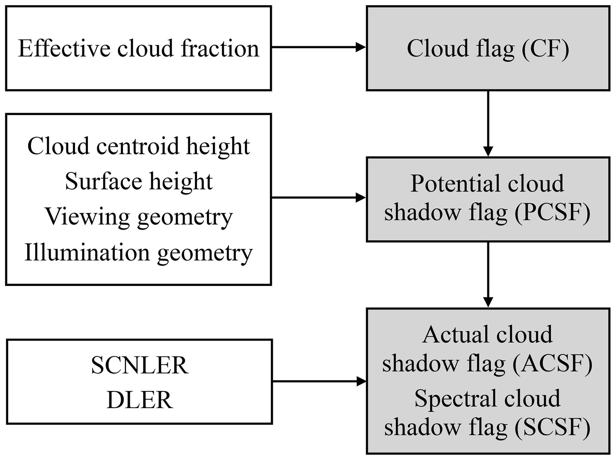
Figure 1 Summary of the inputs and outputs of DARCLOS. The white boxes describe the main input data, and the grey boxes describe the calculated output products. SCNLER refers to the reflectivity of the scene (Sect. 2.2.1), and DLER refers to the climatological directionally dependent surface reflectivity (Sect. 2.2.2). More details are provided in the main text.

2.1 Potential cloud shadow flag (PCSF)

The PCSFs indicate the pixels that are potentially affected by cloud shadows. The PCSF is intended to be useful for filtering any cloud-shadow-contaminated TROPOMI data. Therefore, the number of false negative shadow detections in the PCSF should be minimized (see Sect. 4). Hence, the PCSF shadow is an overestimation of the true shadowed area.

The PCSF is computed in two steps. First, we compute the maximum potential geometric shadow extent from the cloud, with additional safety margins. Then, we flag the area between the cloud and the maximum potential shadow extent. Both steps are explained in more detail below.

2.1.1 The maximum potential shadow extent

Figure 2 illustrates the cloud shadow geometry in the local reference frame at the Earth's surface. The reference frame is equivalent to the topocentric reference frame of TROPOMI (see Loots et al., 2017), except for the xy plane, which is now lifted in the zenith direction with the surface height h_sfc with respect to the WGS84 Earth reference ellipsoid. Here, the origin (point O) of the reference frame is set at the centre of a cloud pixel, which represents the projection of the cloud's centroid in the viewing direction onto the Earth's surface at geodetic latitude δ_c and longitude ϑ_c. The cloud pixels are the TROPOMI ground pixels with a raised cloud flag (CF) and are determined by an effective cloud fraction (the cloud fraction assuming a cloud albedo of 0.8) larger than 0.05. The effective cloud fraction was determined in the NO₂ spectral window and taken from the TROPOMI NO₂ data product (van Geffen et al., 2021). Angles θ₀ and θ are the solar and viewing zenith angles respectively. Angles φ₀ and φ are the solar and viewing azimuth angles respectively, measured positively clockwise from the north when looking in the nadir direction. The values for θ₀, θ, φ₀, and φ are provided in the TROPOMI data for the origin of the unlifted topocentric reference frame, i.e. when h_sfc=0. In the problem of finding the cloud shadow belonging to the cloud pixel at the origin, we neglect variations in θ₀, θ, φ₀, and φ in the horizontal (x and y) and vertical (z) directions, and we assume that h_sfc is constant.

The location, dimensions, and darkness of a cloud shadow cast on the Earth's surface and/or atmosphere below the cloud, as observed from space, may depend on (1) the cloud's location in 3-D space, (2) the location of the underlying surface and/or atmosphere on which the shadow is cast in 3-D space, (3) the horizontal and vertical extents of the cloud, (4) the optical thickness of the cloud, (5) the optical thickness of the atmospheric layers, (6) the illumination geometry (θ₀ and φ₀), and (7) the viewing geometry (θ and φ). Because in the first step of the PCSF determination we search for the maximum potential shadow extent, we assume an opaque cloud and neglect the optical thickness of the atmospheric layers, such that the computed shadows are cast on the Earth's surface where the shadow separation from the cloud is largest.

In Fig. 2, the cloud is located at $(x_{\mathrm{n}},y_{\mathrm{n}},h)$. Point P at $(x_{\mathrm{n}},y_{\mathrm{n}},\mathrm{0})$ is the nadir projection of the cloud's centroid onto the surface, and h is the cloud height with respect to the surface, which can be computed as

$$\begin{array}{}\text{(1)}& h=(\mathrm{1}+C)\left(h_{\mathrm{c}}-h_{\mathrm{sfc}}\right).\end{array}$$

In Eq. (1), h_c is the FRESCO cloud height (Koelemeijer et al., 2001; Wang et al., 2008), which is an approximation of the true height of the cloud's centroid with respect to the WGS84 Earth reference ellipsoid. Because, for the PCSF, we search for the maximum potential shadow extent, we have introduced the safety margin C, which increases the cloud height proportional to h_c−h_sfc. We set C=0.5, for which the number of false negative shadow detections (i.e. the omission error of the PCSF; see Sect. 4) resulting from underestimated maximum potential shadow extents converged to a minimum.

If we assume that the centre of the cloud pixel is the projection of the cloud's centroid in the viewing direction onto the Earth's surface, x_n and y_n can be computed as (see also Luo et al., 2008)

$$\begin{array}{}\text{(2)}& {\displaystyle }{x}_{\mathrm{n}}=h\cdot \tan \mathit{\theta }\sin \mathit{\phi },\text{(3)}& {\displaystyle }{y}_{\mathrm{n}}=h\cdot \tan \mathit{\theta }\cos \mathit{\phi }.\end{array}$$

The location of point Q in the cloud shadow on the Earth's surface, (x_sh,y_sh), then follows from

$$\begin{array}{}\text{(4)}& {\displaystyle }{x}_{\mathrm{sh}}=x_{\mathrm{n}}-h\cdot \tan {\mathit{\theta }}_{\mathrm{0}}\sin {\mathit{\phi }}_{\mathrm{0}},\text{(5)}& {\displaystyle }{y}_{\mathrm{sh}}=y_{\mathrm{n}}-h\cdot \tan {\mathit{\theta }}_{\mathrm{0}}\cos {\mathit{\phi }}_{\mathrm{0}}.\end{array}$$

Finding the geodetic latitude, δ_sh, and longitude, ϑ_sh, of Q is an example of the direct geodetic problem for which the solution involves an iterative procedure (Vincenty, 1975). However, because of the small distances in the cloud shadow geometry relative to the Earth's radii of curvature, δ_sh and ϑ_sh can accurately be approximated by differential northing and easting formulae:

$$\begin{array}{}\text{(6)}& {\displaystyle }{\mathit{\delta }}_{\mathrm{sh}}\approx {\mathit{\delta }}_{\mathrm{c}}+{\displaystyle \frac{y_{\mathrm{sh}}}{M+h_{\mathrm{sfc}}}},\text{(7)}& {\displaystyle }{\mathit{\vartheta }}_{\mathrm{sh}}\approx {\mathit{\vartheta }}_{\mathrm{c}}+{\displaystyle \frac{x_{\mathrm{sh}}}{(N+h_{\mathrm{sfc}})\cos {\mathit{\delta }}_{\mathrm{c}}}},\end{array}$$

where M and N are the Earth's ellipsoidal meridian radius of curvature and radius of curvature in the prime vertical respectively, which both vary with latitude δ_c (see e.g. Torge and Müller, 2012).

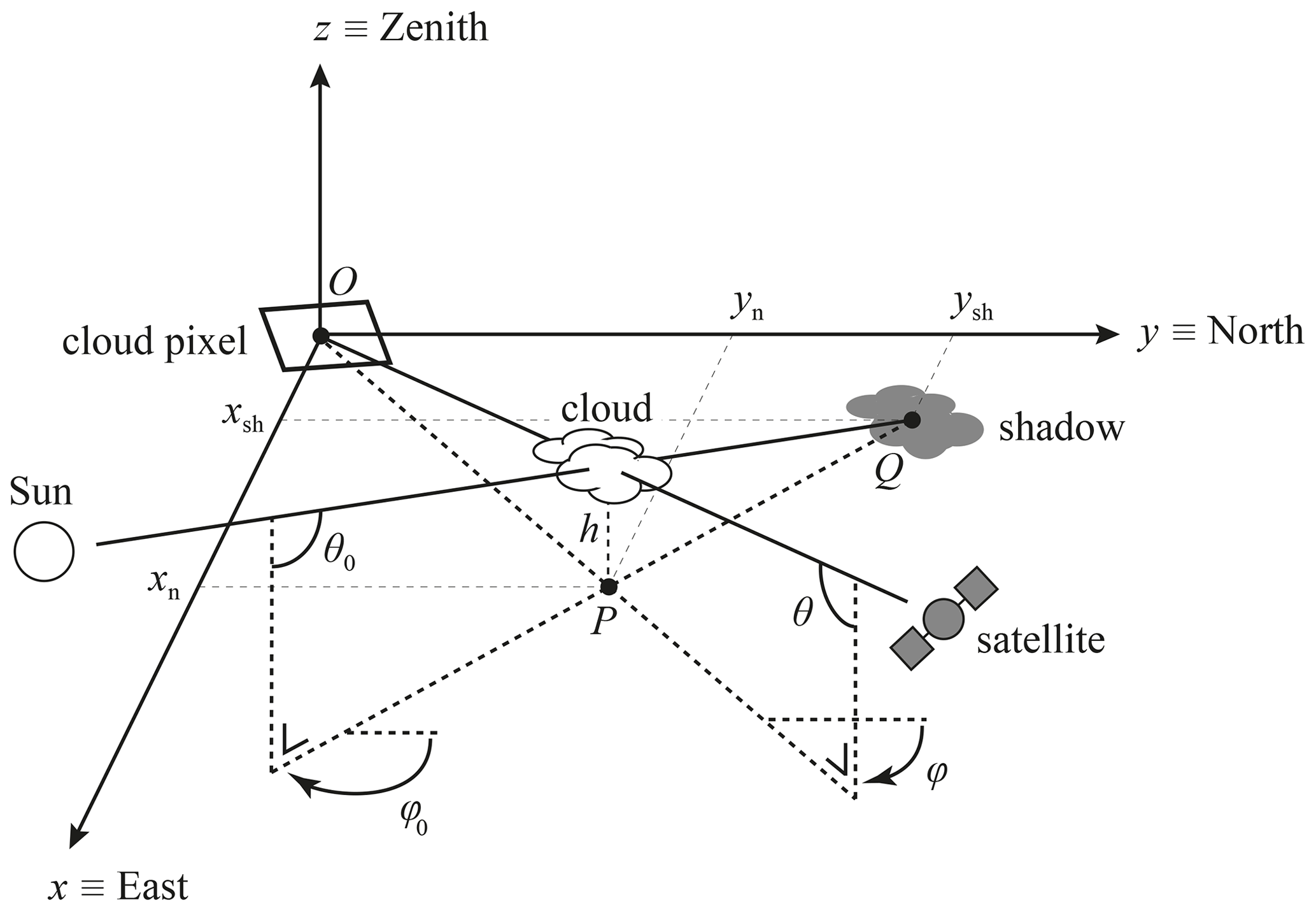
Figure 2 Sketch of the cloud shadow geometry in the local reference frame at the Earth's surface. The cloud as observed by the satellite is located at point O, resulting in a TROPOMI cloud pixel at O (indicated by the white quadrilateral), while the actual cloud is located at height h above point P. The shadow is located at point Q.

The centre of the cloud pixel may not coincide with the projection of the cloud's centroid in the viewing direction onto the Earth's surface, as was assumed in Eqs. (2) and (3). This is particularly true, for example, when small clouds in the pixel are located near the pixel edges or corners, or when the edge of a large cloud deck traverses the pixel. Moreover, the actual projections of the unknown true horizontal and vertical cloud extents are located inside but near the edges of the cloud pixel.² Therefore, we repeat the computation of point Q four times, now placing the corners of the cloud pixel in the origin of the reference frame (not shown in Fig. 2).

2.1.2 Raising the PCSF

In the second step of the PCSF determination, we select the area in which PCSFs are to be raised, based on the calculated points P and Q. As illustrated in Fig. 3, we flag all the cloud-free ground pixels (i.e. for which no CF is raised) within or intersected by the triangle OPQ.

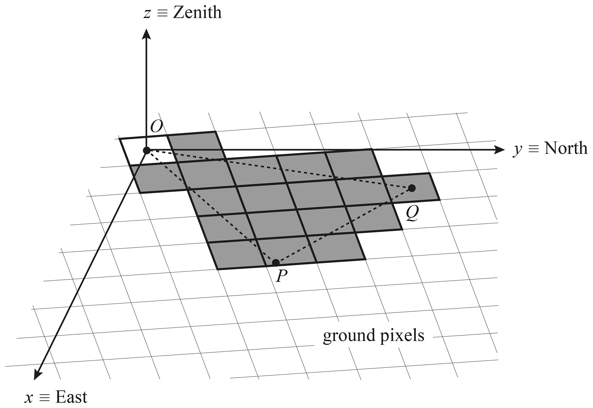
Figure 3 Sketch of the PCSF flagging of the TROPOMI ground pixels in the local reference frame at the Earth's surface. The PCSF pixels are indicated in grey, and the cloud pixel is indicated by the white quadrilateral. Points O, P, and Q correspond to points O, P, and Q in Fig. 2.

All cloud-free ground pixels intersected by line segment OQ are flagged for two reasons. First, OQ is the projection in the viewing direction onto the Earth's surface of a line segment, between the cloud's centroid and point Q, where the shadowed atmosphere is located (e.g. an optically thick atmosphere may lead to short shadows, cast on the atmospheric layers, projected onto the surface close to point O). Secondly, a possible overestimation of h implies an actual cloud's nadir projection closer to O (along line OP), which, with an unchanged illumination geometry, results in a shadow location between O and Q on line segment OQ.

All cloud-free ground pixels intersected by line segment PQ are flagged because the vertical cloud extent below the cloud's centroid is unknown. Although the vertical cloud extent of an isolated cloud may result in an adjacent cloud pixel, the vertical extent below the cloud's centroid may be invisible from space if neighbouring clouds cover the volume below the cloud's centroid. For that reason, line segment PQ represents the potential shadow locations of a hypothetical cloud extending from the cloud's centroid to the surface.

All cloud-free ground pixels within or intersected by triangle OPQ are flagged, because combinations of the aforementioned situations may occur. For similar reasons as mentioned in Sect. 2.1.1, we repeat the flagging four times for the triangles OPQ where O is placed in the corners of the cloud pixel (not shown in Fig. 3).

2.2 Actual cloud shadow flag (ACSF)

In this section, the computation of the ACSF is explained. The ACSFs indicate the pixels that are confidently affected by cloud shadows. They are a subset of the PCSFs and are intended to be useful for selecting pixels for the scientific analysis of cloud shadows. The number of false positive shadow detections in the ACSF should therefore be minimized (see Sect. 4).

The ACSF is determined in two steps. First, we apply a Rayleigh scattering correction to the measured reflectance at the top of the atmosphere for the PCSF pixels. Then, we compare the corrected reflectance to the expected surface reflectance from climatological observations by TROPOMI, revealing the actual shadowed pixels. This comparison is done at the wavelength where the surface reflectance is strongest. Both steps are explained in more detail below.

2.2.1 Lambertian-equivalent reflectivity of the scene (SCNLER)

The spectral Earth's reflectance at the top of the atmosphere (TOA) as measured by a satellite is defined as

$$\begin{array}{}\text{(8)}& R^{\mathrm{meas}}\left(\mathit{\mu },{\mathit{\mu }}_{\mathrm{0}},\mathit{\phi },{\mathit{\phi }}_{\mathrm{0}},\mathit{\lambda }\right)={\displaystyle \frac{\mathit{\pi }I\left(\mathit{\mu },{\mathit{\mu }}_{\mathrm{0}},\mathit{\phi },{\mathit{\phi }}_{\mathrm{0}},\mathit{\lambda }\right)}{{\mathit{\mu }}_{\mathrm{0}}{E}_{\mathrm{0}}\left(\mathit{\lambda }\right)}},\end{array}$$

where I is the radiance reflected by the atmosphere–surface system in W m⁻² sr⁻¹ nm⁻¹, E₀ is the extraterrestrial solar irradiance perpendicular to the beam in W m⁻² nm⁻¹, and μ₀=cos θ₀. I and E₀ depend on wavelength λ in nanometres, and I additionally depends on μ=cos θ, μ₀, φ, and φ₀.

First, we calculate the albedo of the surface, A_s, needed to match a modelled TOA reflectance, R^model, to the measured TOA reflectance, R^meas. The model assumes a Lambertian (i.e. depolarizing and isotropic reflecting) surface below a cloud-free and aerosol-free atmosphere, such that the modelled TOA reflectance can be expressed as (Chandrasekhar, 1960)

$$\begin{array}{}\text{(9)}& \begin{array}{rl}{R}^{\mathrm{model}}\left(\mathit{\mu },{\mathit{\mu }}_{\mathrm{0}},\mathit{\phi }-{\mathit{\phi }}_{\mathrm{0}},\mathit{\lambda }\right)=& R^{\mathrm{0}}\left(\mathit{\mu },{\mathit{\mu }}_{\mathrm{0}},\mathit{\phi }-{\mathit{\phi }}_{\mathrm{0}},\mathit{\lambda }\right)\\ & +{\displaystyle \frac{A_{\mathrm{s}}\left(\mathit{\lambda }\right)T(\mathit{\mu },{\mathit{\mu }}_{\mathrm{0}},\mathit{\lambda })}{\mathrm{1}-A_{\mathrm{s}}\left(\mathit{\lambda }\right)s^{*}\left(\mathit{\lambda }\right)}}.\end{array}\end{array}$$

The first term at the right-hand side of Eq. (9), R⁰, is the so-called path reflectance, which is the modelled TOA reflectance of the atmosphere bounded below by a black surface. The second term is the modelled surface contribution to the TOA reflectance, where A_s is the albedo of the Lambertian surface, T is the total transmittance of the atmosphere for illumination from above and below, and s^* is the spherical albedo of the atmosphere for illumination from below. Quantities R⁰, T, and s^* of the cloud-free and aerosol-free atmosphere–surface model were prepared with the “Doubling-Adding KNMI” (DAK) radiative transfer code (de Haan et al., 1987; Stammes, 2001), version 3.2.0, taking into account single and multiple Rayleigh scattering of sunlight by molecules in a pseudo-spherical atmosphere, including polarization. Absorption by O₃, NO₂, O₂, H₂O, and the O₂–O₂ collision complex was taken into account. For more details about the computation of the quantities in Eq. (9), we refer to Tilstra (2022).

The albedo A_s for which R^model(λ)=R^meas(λ) holds is in this paper indicated by A_scene. The expression for A_scene follows from Eq. (9) (see e.g. Tilstra et al., 2017):

$$\begin{array}{}\text{(10)}& A_{\mathrm{scene}}\left(\mathit{\lambda }\right)={\displaystyle \frac{R^{\mathrm{meas}}\left(\mathit{\lambda }\right)-R^{\mathrm{0}}\left(\mathit{\lambda }\right)}{T\left(\mathit{\lambda }\right)+s^{*}\left(\mathit{\lambda }\right)\left(R^{\mathrm{meas}}\right(\mathit{\lambda })-R^{\mathrm{0}}(\mathit{\lambda }\left)\right)}},\end{array}$$

where the notation for the dependency on μ, μ₀, φ, and φ₀ is omitted. We compute A_scene for λ= 402, 416, 425, 440, 463, 494, 670, 685, 696.97, 712.7, 747, 758, and 772 nm and co-register the results at NIR wavelengths to the Level 2 UVIS ground pixel grid. The values of A_scene can be interpreted as the TOA reflectances of the scene corrected for molecular Rayleigh scattering. They are in fact scene albedos, because they include non-Lambertian surface, aerosol, cloud, and shadow effects. Therefore, in what follows, we refer to A_scene as the Lambertian-equivalent reflectivity of the scene (SCNLER). Only in the absence of non-Lambertian effects, is A_scene independent of μ, μ₀, φ, and φ₀ and approximates the true surface albedo.

2.2.2 Directionally dependent Lambertian-equivalent reflectivity (DLER) climatology

In the second step of the ACSF determination, the SCNLER of the PCSF pixels is compared to climatological observations at the same coordinates and time of the year. For the climatological observations, we use the directionally dependent Lambertian-equivalent reflectivity (DLER) data³ version 0.6 generated with TROPOMI observations of the SCNLER since the start of TROPOMI's operational phase in May 2018. The DLER is available on a global $\mathrm{0.125}{}^{\circ }\times \mathrm{0.125}{}^{\circ }$ resolution latitude–longitude grid for each calendar month at 21 1 nm wide wavelength bins between 328 and 2314 nm (Tilstra, 2022). We linearly interpolate the DLER data to the TROPOMI Level 2 UVIS ground pixel grid and measurement times. Unless stated otherwise, the wavelength bins we use are centred at 402, 416, 425, 440, 463, 494, 670, 685, 696.97, 712.7, 747, 758, and 772 nm.

In the DLER algorithm, an initial cloud screening was performed on the basis of NPP-VIIRS cloud information. After that, the 10 % lowest SCNLER measurements in the seasonal grid cell were used, which serves as a second-stage cloud filter, and measurements containing aerosols were excluded (see Tilstra, 2022). The DLER can generally be considered shadow-free. The DLER takes into account the viewing zenith angle dependence of the SCNLER caused by non-Lambertian surface reflectance. The DLER is a more accurate estimate of the expected aerosol-, cloud-, and shadow-free SCNLER than the traditionally used LER (without viewing zenith angle dependence). The viewing zenith angle dependence of the DLER is only taken into account over land surfaces. Over water surfaces, DLER is equal to LER. For more details about the DLER theory, we refer to Tilstra et al. (2021).

2.2.3 Raising the ACSF

In order to select the pixels for which an ACSF is to be raised, we define the SCNLER–DLER contrast parameter Γ:

$$\begin{array}{}\text{(11)}& \mathrm{\Gamma }\left(\mathit{\lambda }\right)={\displaystyle \frac{A_{\mathrm{scene}}\left(\mathit{\lambda }\right)-A_{\mathrm{DLER}}\left(\mathit{\lambda }\right)}{A_{\mathrm{DLER}}\left(\mathit{\lambda }\right)}}\times \mathrm{100}\mathit{\%}.\end{array}$$

The division by A_DLER (the value of the DLER) in Eq. (11) allows us to search for a A_DLER-independent ACSF threshold for Γ, that is, a single threshold that can be used for both dark and bright surface types. Because of the division by the DLER, Γ is more stable (i.e. less susceptible to potential offset errors in the DLER) when the DLER is high. For each PCSF pixel, we compute the wavelength for shadow detection, λ_max, at which the pixel's DLER is maximum:

$$\begin{array}{}\text{(12)}& {\mathit{\lambda }}_{\max }=\underset{\mathit{\lambda }}{\text{argmax}}{A}_{\mathrm{DLER}}\left(\mathit{\lambda }\right).\end{array}$$

We raise an ACSF at PCSF pixels for which

$$\begin{array}{}\text{(13)}& \mathrm{\Gamma }\left({\mathit{\lambda }}_{\max }\right)<q,\end{array}$$

where q is the contrast threshold. We set $q=-\mathrm{15}$ %, yielding the highest actual shadow detection score in the validation (see Sect. 4).

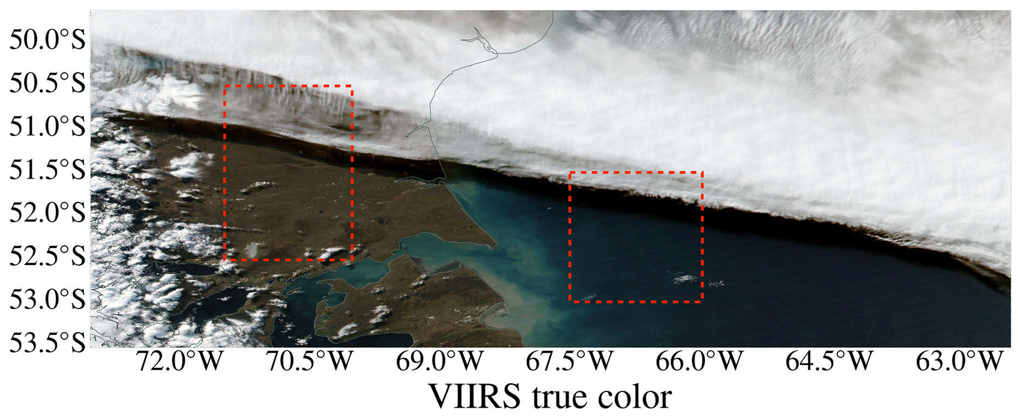
Figure 4 VIIRS-NPP true-colour image of southern Chile and Argentina on 3 August 2019. The land and water regions belonging to the spectra of Fig. 5 are indicated by red dashed boxes.

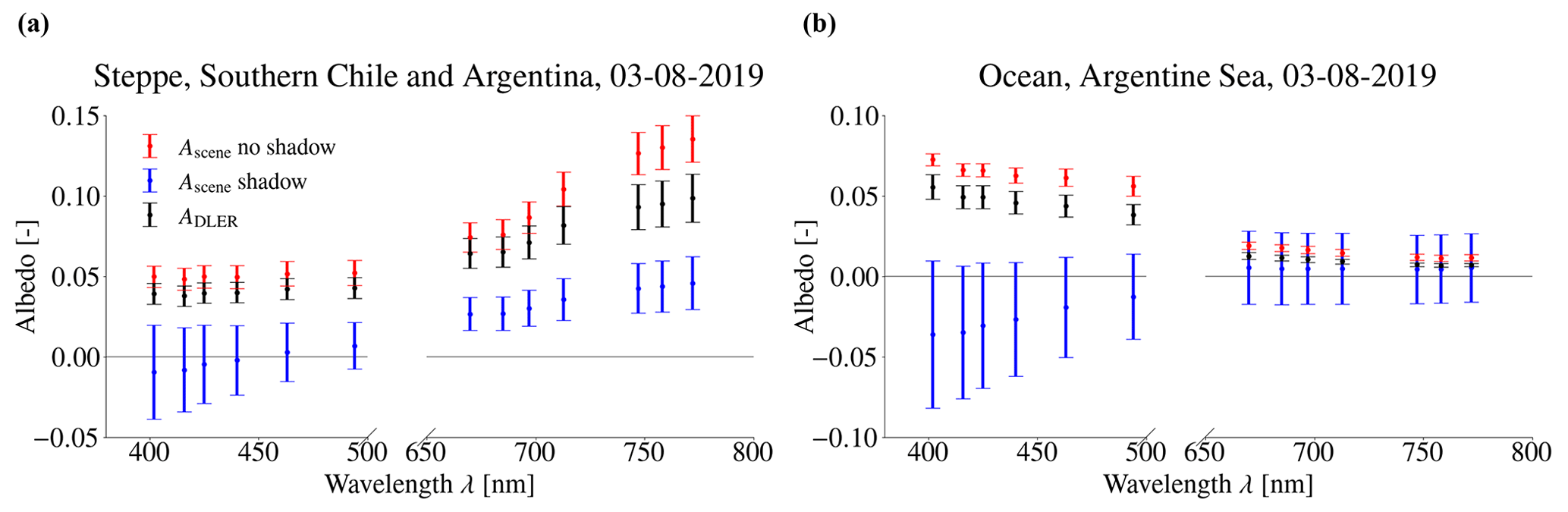
Figure 5 Spectra of the mean and 1σ of the Lambertian-equivalent scene reflectivity (SCNLER) measured by TROPOMI at southern Chile and Argentina on 3 August 2019, for the steppe region within 52.5–50.5^∘ S latitude and 71.5–70^∘ W longitude (a) and for the ocean region within 53–51.5^∘ S latitude and 67.5–66^∘ W longitude (b). Here, all measurements are cloud-free (i.e. without CF). The measurements affected by shadow (i.e. with ACSF) are presented in blue, and the shadow-free measurements (i.e. without PCSF) are presented in red. The additional black spectra are of the mean and 1σ of the directionally dependent climatological Lambertian-equivalent reflectivity (DLER) at the TROPOMI ground pixels in the particular regions.

2.2.4 Rationale behind the SCNLER–DLER contrast parameter

Here, we demonstrate the behaviour of the variables in Eqs. (11) to (13) which determine the SCNLER–DLER contrast parameter Γ with an example measurement. Figure 4 is a true-colour image made by the Visible Infrared Imager Radiometer Suite (VIIRS) instrument on board the Suomi National Polar-orbiting Partnership (NPP) satellite, on 3 August 2019 above southern Chile and Argentina. Suomi NPP orbits in close proximity to Sentinel-5P: the measurement time intervals of TROPOMI and VIIRS were 19:00–19:01 and 18:57–18:58 UTC respectively. A specific land region (52.5–50.5^∘ S latitude and 71.5–70^∘ W longitude) and water region (53–51.5^∘ S latitude and 67.5–66^∘ W longitude) are indicated by red dashed boxes. The main surface types in those regions are steppe and ocean respectively. Figure 5a and b show the spectral behaviour of the mean and 1σ of SCNLER measurements affected by shadow (A_scene shadow) and not affected by shadows (A_scene no shadow) of cloud-free TROPOMI pixels in the land and water regions respectively. We used the PCSF to remove shadow pixels and the ACSF to select shadow pixels. Also shown are the mean and 1σ of the DLER interpolated on the TROPOMI Level 2 UVIS grid.

Figure 5a shows that over land (steppe), the DLER and the cloud- and shadow-free SCNLER follow a typical surface reflectivity spectrum for grasslands (see Fig. 7 of Tilstra et al., 2017): they increase with increasing wavelength and include a subtle signature of the so-called “red edge” (i.e. the sudden surface albedo increase at λ∼700 nm caused by vegetation). Over ocean, the DLER and cloud- and shadow-free SCNLER follow a typical surface reflectivity spectrum for ocean water: they increase with decreasing wavelength and peak at λ∼400 nm where the peak significance depends on the water constituents (see also e.g. Morel and Maritorena, 2001). The mean value of A_scene affected by shadow is smaller than the DLER and cloud- and shadow-free A_scene at all wavelengths, for both the land and water regions. The shadow signature in the difference A_scene−A_DLER is most evident at the wavelength where the DLER is highest. The Rayleigh scattering correction results in negative A_scene for part of the shadowed pixels. Above land, a slight increase in the shadowed A_scene can still be observed with increasing wavelength, but above ocean, the water albedo increase in the UV cannot be observed anymore. Note that the mean DLER is consistently smaller than the mean cloud- and shadow-free SCNLER measured at all wavelengths, which is expected since the DLER at a certain location was generated with the 10 % lowest SCNLER values at that location.

Figure 6a shows λ_max on the TROPOMI Level 2 UVIS ground pixel grid for this measurement example. As expected from Fig. 5, λ_max=772 nm for the majority of the land-covered pixels, and λ_max=402 nm for the majority of the water-covered pixels. In shallow water regions near the coast line, however, λ_max=494 nm, while in some land coast regions we find λ_max=670 nm. Indeed, employing λ_max, the usage of surface type classification flags is avoided (see Romahn et al., 2021, for an example of surface type classification flags usage). That is, λ_max does not rely upon assumptions made in a surface type classification product and will also give the most suitable wavelength for shadow detection when mixed and/or rare surface types are present within the pixel.

Figure 6 The wavelength at which DLER is maximum λ_max (a), the SCNLER at λ_max (b), the DLER at λ_max (c), and contrast parameter Γ at λ_max (d), for southern Chile and Argentina on 3 August 2019.

Figure 6b, c, and d show A_scene, A_DLER, and Γ respectively at λ_max. Cloud- and shadow-free pixels yield Γ(λ_max)∼0 % or slightly positive (up to ∼50 %), because the DLER is generated with the 10 % lowest SCNLER values in the particular calendar month that passed an aerosol and cloud screening. The clouds at latitudes larger than 52.5^∘ increase A_scene significantly relative to A_DLER , which results in Γ(λ_max)>50 %. Pixels affected by true shadows show a significantly decreased A_scene relative to A_DLER, which is most apparent for the elongated cloud shadow along the edge of the cloud deck.

3 Results

Here, we discuss the potential and actual cloud shadow flag results for three case studies with different cloud and surface types: the cloud deck example above steppe and ocean surfaces introduced in Sect. 2.2.4 (Sect. 3.1), an example with patchy clouds above grass and forest surfaces (Sect. 3.2), and an example of a relatively large area above the Sahara containing thin cirrus clouds (Sect. 3.3).

3.1 Southern Chile and Argentina, 3 August 2019

Figure 7a and b show (in blue) the TROPOMI Level 2 UVIS ground pixels with raised PCSFs and ACSFs respectively for the cloud shadow example on 3 August 2019 at southern Chile and Argentina.

Figure 7 The TROPOMI Level 2 UVIS ground pixels for southern Chile and Argentina on 3 August 2019 with raised PCSFs (Fig. 7a) and with raised ACSFs (Fig. 7b), indicated in blue. The white pixels are cloud pixels, and grey pixels do not contain a raised cloud or shadow flag.

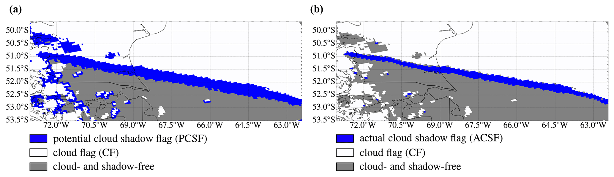
Figure 7a shows that the PCSFs indicate the presence of an elongated cloud shadow southward of the edge of the cloud deck longitudinally traversing the scene from ∼51 to ∼52.5^∘ S latitude. The southward shadow is expected because in this example the Sun is located in the northwest (φ₀ ranges from −29.3^∘ in the west to −41.7^∘ in the east). The Sun is located relatively low in the sky because of the local winter season (θ₀ ranges from 72.2^∘ in the northwest to 79.7^∘ in the southeast), which is geometrically beneficial for the existence of long shadows (see Eq. 5). The latitudinal extent of the elongated shadow is relatively large compared to the shadows of the isolated small clouds found at latitudes southward of 51.5^∘ S. This variation in shadow extent can be explained by the difference in cloud height: h∼15 km for the cloud deck and h∼1 km for the isolated small clouds. The cloud deck shadow extent is larger than expected from visual inspection of the true-colour image (Fig. 4), which is caused by the cloud height safety margin C that we included in Eq. (1).

Figure 7b shows that the latitudinal extent of the cloud deck shadow detected with the ACSF is a more realistic approximation of the latitudinal cloud deck shadow extent observed in the true-colour image of Fig. 4. Only a few shadows of small isolated clouds are detected by the ACSF. Note that part of the small isolated clouds are in fact false positive cloud detections in the cloud product caused by bright surfaces. This can readily be concluded by comparing Fig. 7b to Fig. 4. For example, the water constituents along the coast between 53 and 53.5^∘ S latitude, but also the snowy mountains westward of 71^∘ W, are falsely interpreted as clouds. These false cloud shadow detections in the PCSF are correctly filtered out by the threshold for Γ(λ_max) (Eq. 13) and are therefore not part of the ACSF. Indeed, the performance of the shadow detection algorithm depends on the quality of the input cloud and DLER products. The gaps in the cloud deck between 51 and 50^∘ S are caused by undefined cloud fractions in the cloud product, but again, the false PCSF shadow detections within those gaps are (except for 2 pixels) correctly removed from the ACSF.

3.2 The Netherlands and Germany, 18 November 2018

Figure 8a and c show the true-colour image and the TROPOMI Level 2 UVIS ground pixels with raised PCSFs respectively for an example on 18 November 2018 above the Netherlands and Germany. TROPOMI orbits northwestward, and the viewing geometry is southwestward: θ ranges from 8.8^∘ in the northeast to 54.3^∘ in the southwest. The Sun is located in the south (φ₀ ranges from −180.0^∘ in the west to −165.7^∘ in the east) and the solar zenith angle θ₀ ranges from 65.8^∘ in the south to 76.8^∘ in the north.

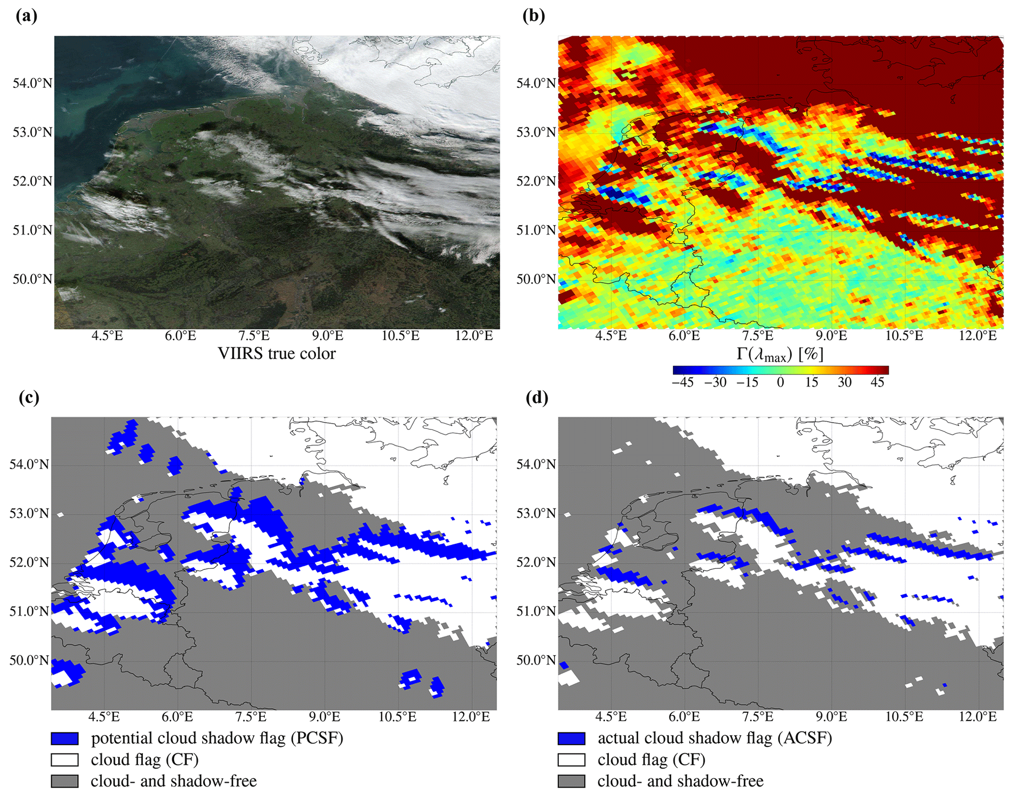
Figure 8 VIIRS-NPP true-colour image (a), SCNLER–DLER contrast parameter Γ at λ_max measured by TROPOMI (b) and TROPOMI Level 2 UVIS ground pixels with raised PCSFs (c) and with raised ACSFs (d), for the Netherlands and Germany on 18 November 2018. In (c, d) white pixels are cloud pixels, and grey pixels do not contain a raised cloud or shadow flag.

With the PCSF, long potential cloud shadows are found extending towards the northeast. Here, all clouds that produce shadows are relatively high (h∼10 km or higher). Note that at the location of the small isolated clouds above the sea at ∼54^∘ N latitude and 4.5–6^∘ E longitude, the Sun is almost directly located in the south. The eastward component of the potential shadow at these longitudes is caused by the parallax effect (see Fig. 2): the southwestward-looking instrument projects the cloud as a cloud pixel onto the surface southwestward from the cloud's actual nadir location. Although the path from the cloud's nadir location to the actual shadow is strictly northward, the path from the cloud pixel to the actual shadow is northeastward.

The majority of the cloud shadows in this example are found above land surface. The main land surface types in this part of Europe are grassland and forest, with in general a higher vegetation density than for the steppe land in the example shown in Sect. 3.1. Consequently, the red edge is more pronounced in this example, resulting in a stronger surface reflectance in the near-infrared. Hence, we find that λ_max=772 nm for all pixels over land. The relatively high surface reflectance in the near-infrared results in a clear shadow signature in Γ(λ_max) (see Fig. 8b): in the cloud- and shadow-free regions Γ(λ_max) equals 0 or is slightly positive, while strong negative Γ(λ_max) values are confined to cloud shadows (see Fig. 8a).

Figure 8d shows the TROPOMI Level 2 UVIS ground pixels with raised PCSFs for this example. Comparing the shadows detected with the ACSF to the true-colour image of Fig. 8a shows that ACSF shadows are detected where they can be expected. The small high isolated clouds above the sea do not produce dark enough shadows for an ACSF to be raised, similar to the small high isolated clouds above land at ∼49.5^∘ N latitude and ∼10.5 to 11^∘ E longitude.

3.3 Sahara, 18 January 2021

Figure 9 is equivalent to Fig. 8, but then for an example above the Sahara on 18 January 2021. The area of this example covers most of the orbit swath of TROPOMI travelling north-northwestward: θ ranges from 66.5^∘ in the west-southwest to −58.1^∘ in the east-northeast. Although the latitudes in this example are relatively small, the local winter season causes the Sun not to be located directly overhead (θ₀ ranges from 28.4^∘ in the south to 59.3^∘ in the north, and φ₀ ranges from −178.7^∘ in the west to −140.3^∘ in the east).

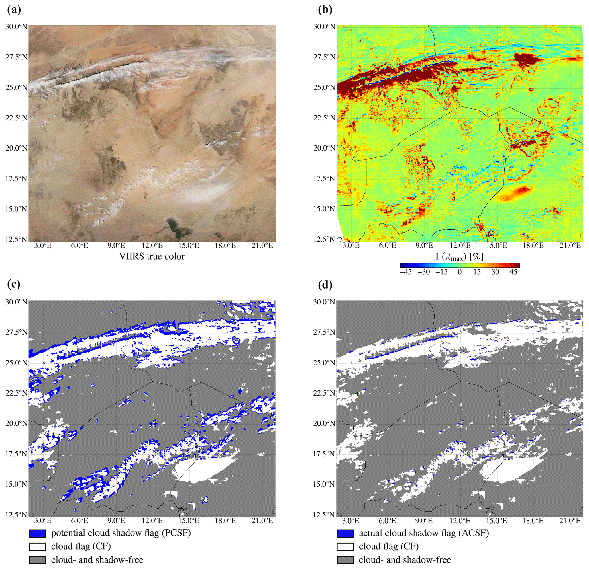
Figure 9 Similar to Fig. 8, but for the Sahara on 18 January 2021.

With the PCSF, northward shadows of longitudinally elongated cirrostratus clouds between 25 and 28^∘ N latitude and of cirrocumulus clouds between 13 and 22.5^∘ N latitude are detected. For both cloud types, h>10 km. The vertical location of the detected foggy patch at 15–17.5^∘ N latitude and 14–19^∘ E longitude is just above the surface, hence the absence of the potential shadow (see Fig. 9c). This example is a clear demonstration of the parallax effect: on the west side of the area, TROPOMI looks westward, projecting the clouds as cloud pixels onto the surface “too far” westward, resulting in an eastward component of the potential shadow locations with respect to the cloud pixels. Similarly, on the east side of the area, TROPOMI looks eastward, and potential shadows tend to be located westward of the cloud pixels.

With the ACSF, the detected shadows are a more accurate approximation of the shadows observed in the true-colour image (see Fig. 9d and a). The most distinctive shadow signature in the true-colour image, which is the northward shadow of the longitudinally elongated cirrostratus cloud between 25 and 27^∘ N latitude, is indeed also detected by the ACSF. Although, geometrically, many other clouds in this example are high enough to produce potential cloud shadows, some of those clouds are too small and/or too thin to produce actual cloud shadows. This can be seen in Fig. 9b: for example, the cirrocumulus clouds near 13.5^∘ N latitude and 4.5^∘ E longitude are not able to decrease Γ(λ_max) significantly enough for an ACSF to be raised.

The spectral reflectance of desert surface does not contain a red edge but is relatively strong already at λ<700 nm and further increases with increasing wavelength (see e.g. Fig. 7 of Tilstra et al., 2017). We find that for almost all pixels in this example, λ_max=772 nm. Comparing Fig. 9b with the false colour image of Fig. 9a shows that strong negative Γ(λ_max) values are strictly confined to cloud shadows (except for a few pixels near 12.7^∘ N latitude and 17.8^∘ E longitude). The cloud- and shadow-free area yield Γ(λ_max)∼0 or are slightly positive. That is, dark surface features in the Sahara are not falsely detected as cloud shadows.

4 Validation

In this section, we validate DARCLOS by comparing the computed PCSFs and ACSFs to the shadows visually found at similar locations and time in VIIRS-NPP true-colour images. For the visual inspection of the true-colour images, we have developed an interactive Python tool which plots the TROPOMI Level 2 UVIS grid on top of the true-colour image. The software allows for the manual selection and de-selection of TROPOMI pixels containing VIIRS shadows by clicking on the image, after which the row and scanline numbers of the selected TROPOMI pixels are saved.

Figure 11a shows a VIIRS-NPP true-colour image of cloud shadows found at the Taklamakan Desert at Xinjiang, China, on 22 December 2019. The red lines represent the TROPOMI Level 2 UVIS grid, and the blue crosses indicate the TROPOMI pixels with a raised ACSF. If, also, a VIIRS shadow is visually found at the TROPOMI pixel with a raised shadow flag, we speak of a true positive (TP) shadow detection. Similarly, we register the false positive (FP), false negative (FN), and true negative (TN) shadow detections (see Fig. 10).

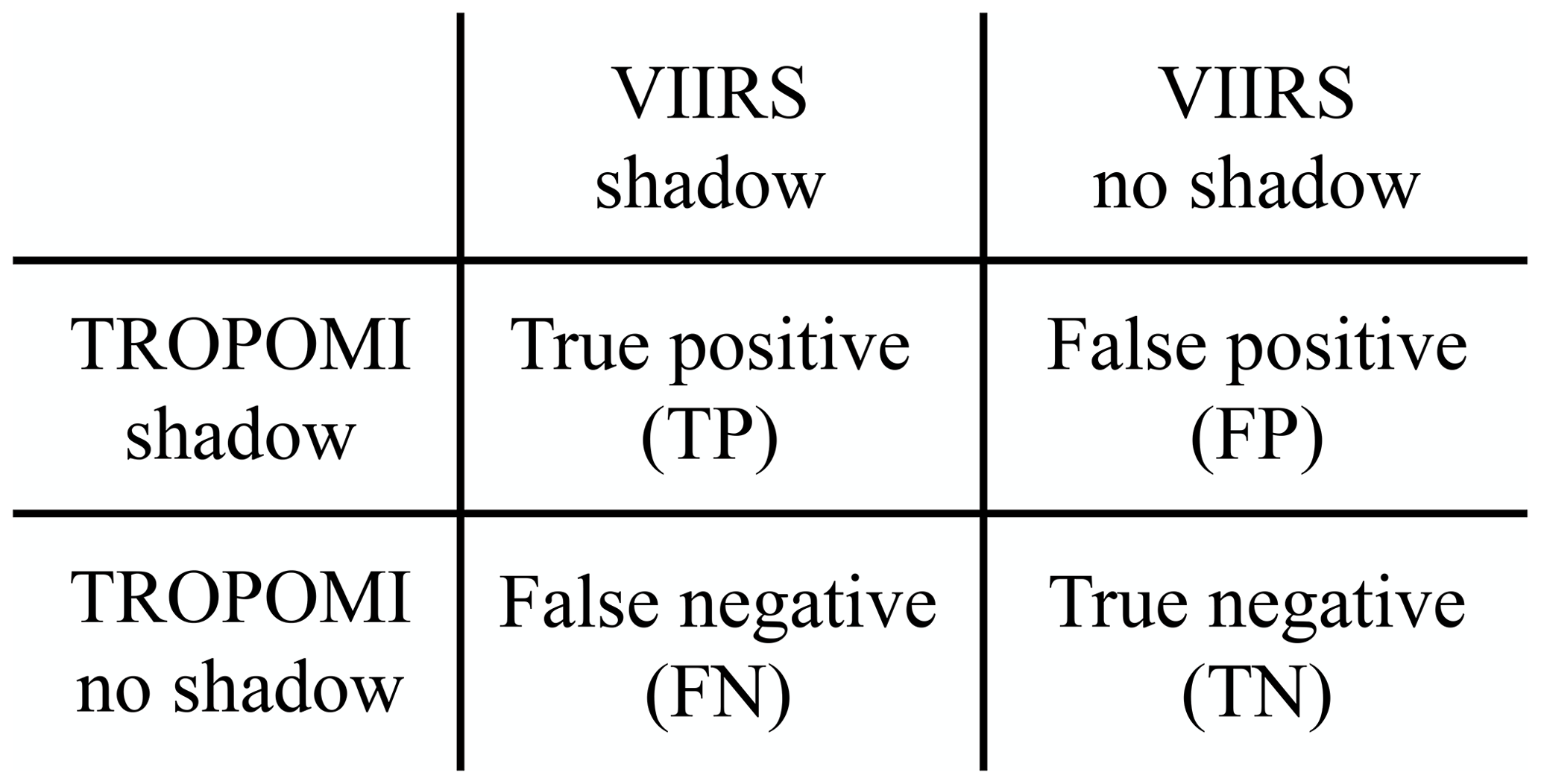
Figure 10 Confusion matrix of the shadow detection on the TROPOMI Level 2 UVIS grid. TROPOMI shadows are detected with the PCSF or ACSF of DARCLOS. VIIRS shadows are manually determined by visual inspection of VIIRS true-colour images.

Figure 11 VIIRS-NPP true-colour image of the Taklamakan Desert at Xinjiang, China, 22 December 2019, with the TROPOMI Level 2 UVIS grid plotted on top (in red) and the detected ACSF by DARCLOS (blue crosses), uncorrected (a) and at the VIIRS measurement times (b). Panels (c, d) show respectively the eastward and northward atmospheric movement at the cloud height during the TROPOMI–VIIRS measurement time difference, computed using ERA5 reanalysis wind data.

The overestimation of the VIIRS shadow by DARCLOS can be expressed by the commission error, ϵ_C (see also e.g. Candra et al., 2016):

$$\begin{array}{}\text{(14)}& {\mathit{ϵ}}_{\mathrm{C}}={\displaystyle \frac{N_{\mathrm{FP}}}{N_{\mathrm{TP}}+N_{\mathrm{FP}}}},\end{array}$$

where N_FP and N_FN are the number of false positive detections and the number of false negative detections respectively. The underestimation of the VIIRS shadow by DARCLOS can be expressed by the omission error, ϵ_O:

$$\begin{array}{}\text{(15)}& {\mathit{ϵ}}_{\mathrm{O}}={\displaystyle \frac{N_{\mathrm{FN}}}{N_{\mathrm{TP}}+N_{\mathrm{FN}}}},\end{array}$$

where N_FN are the number of false negative detections. For the definition of the VIIRS shadows, we distinguish between TROPOMI pixels that are totally shadowed (with geometrical shadow fractions ≳0.75) and partly shadowed (with geometrical shadow fractions ≳0 and ≲0.75). For the computation of ϵ_O, we use only the totally shadowed pixels, while for the computation of ϵ_C, we use both the totally and partly shadowed pixels. That is, we consider the underestimation of the totally shadowed pixels, and the overestimation of the totally and partly shadowed pixels, to be erroneous. The overall performance of the algorithm can be assessed with the F₁ score, which combines ϵ_C and ϵ_O as follows (see e.g. Fernández et al., 2018):

$$\begin{array}{}\text{(16)}& F_{\mathrm{1}}={\displaystyle \frac{\mathrm{2}\left(\mathrm{1}-{\mathit{ϵ}}_{\mathrm{C}}\right)\left(\mathrm{1}-{\mathit{ϵ}}_{\mathrm{O}}\right)}{\left(\mathrm{2}-{\mathit{ϵ}}_{\mathrm{C}}-{\mathit{ϵ}}_{\mathrm{O}}\right)}}.\end{array}$$

In the hypothetical case of a perfect shadow detection, we would obtain ϵ_O=0, ϵ_C=0, and F₁ score =1. For the ACSF in a slightly larger area than shown in Fig. 11a (36.5–43.0^∘ N, 76.0–88.0^∘ E), the results are ϵ_O=0.27, ϵ_C=0.21 and F₁ score =0.76.

It can be observed that the TROPOMI pixels with a raised ACSF in Fig. 11a are consistently located slightly eastwards of the shadows found in the VIIRS true-colour image. The eastward shift can be explained by the motion of the clouds during the measurement time difference of TROPOMI and VIIRS. In the example of Fig. 11, the VIIRS measurements were on average taken 4.33 min ahead of the TROPOMI measurements, with a 1σ of 0.07 min⁴. We interpolate ERA5 data (Hersbach et al., 2018) of hourly eastward and northward wind speed components, provided at 37 vertical pressure levels on a $\mathrm{0.25}{}^{\circ }\times \mathrm{0.25}{}^{\circ }$ latitude–longitude grid, onto the FRESCO cloud pressure on the TROPOMI Level 2 UVIS grid (i.e. without manually raising the cloud height such as in Eq. 1). The cloud deck in the southwest in Fig. 11 is relatively high (the cloud pressure is ∼400 hPa), where eastward wind speeds between 20 and 40 m s⁻¹ are found. The eastward and northward cloud displacements are shown in Fig. 11c and d respectively. The cloud displacements from ∼6 to ∼9 km are significant enough to shift some clouds, and hence some cloud shadows, at least one TROPOMI ground pixel in the eastward direction.⁵

In Fig. 11b we have corrected the locations of the TROPOMI cloud and cloud shadow pixels for the eastward and northward movement of the clouds during the TROPOMI–VIIRS measurement time difference. Note the much better agreement between the ACSF and the VIIRS shadows compared to Fig. 11a. Indeed, using the corrected ACSF, the errors decreased and the F₁ score increased: ϵ_O=0.08, ϵ_C=0.02, and F₁ score =0.95. It should be noted that the validation may suffer from an imperfect correction of the cloud movement during the TROPOMI–VIIRS measurement time difference, because the cloud evolution is ignored and because of the relatively coarse resolution of the wind product. Therefore, we expect the true shadow detection performance at the TROPOMI measurement time to be even better than the performance presented with this validation.

The last three columns of Table 1 show the results for ϵ_O, ϵ_C, and the F₁ score of the ACSF for the three examples discussed in this paper, and three additional examples (on 22 December 2019, 9 October 2018, and 21 December 2020) not shown in this paper. The F₁ score is 0.84 or higher for all examples. The F₁ score is highest (0.94 and 0.95 respectively) for southern Chile and Argentina, 3 August 2019, and for the Taklamakan Desert, 22 December 2019. The shadows in those examples are caused by relatively large and thick cloud decks and are therefore relatively distinctive. The examples with the lowest F₁ scores (0.84 and 0.86 respectively) are the Sahara, 18 January 2021, and the Netherlands, Belgium, and Luxembourg, 9 October 2018. The shadows in those examples are caused by relatively thin and small clouds and are therefore relatively subtle. Subtle shadows lead to less distinctive shadow signatures in Γ, leading to more false negative shadow detections and a higher ϵ_O of the ACSF. Also, thin and/or small clouds are sometimes not detected by the cloud product because the cloud fraction is too low to raise a CF, resulting in false negative PCSFs and ACSFs. Moreover, we speculate that thinner and/or smaller clouds are more likely to appear and disappear during the TROPOMI–VIIRS measurement time difference, complicating the cloud movement correction and validation of these examples.

Table 1 Results of the validation of the PCSF and ACSF by inspection of VIIRS-NPP true-colour images. The final results are shown in bold.

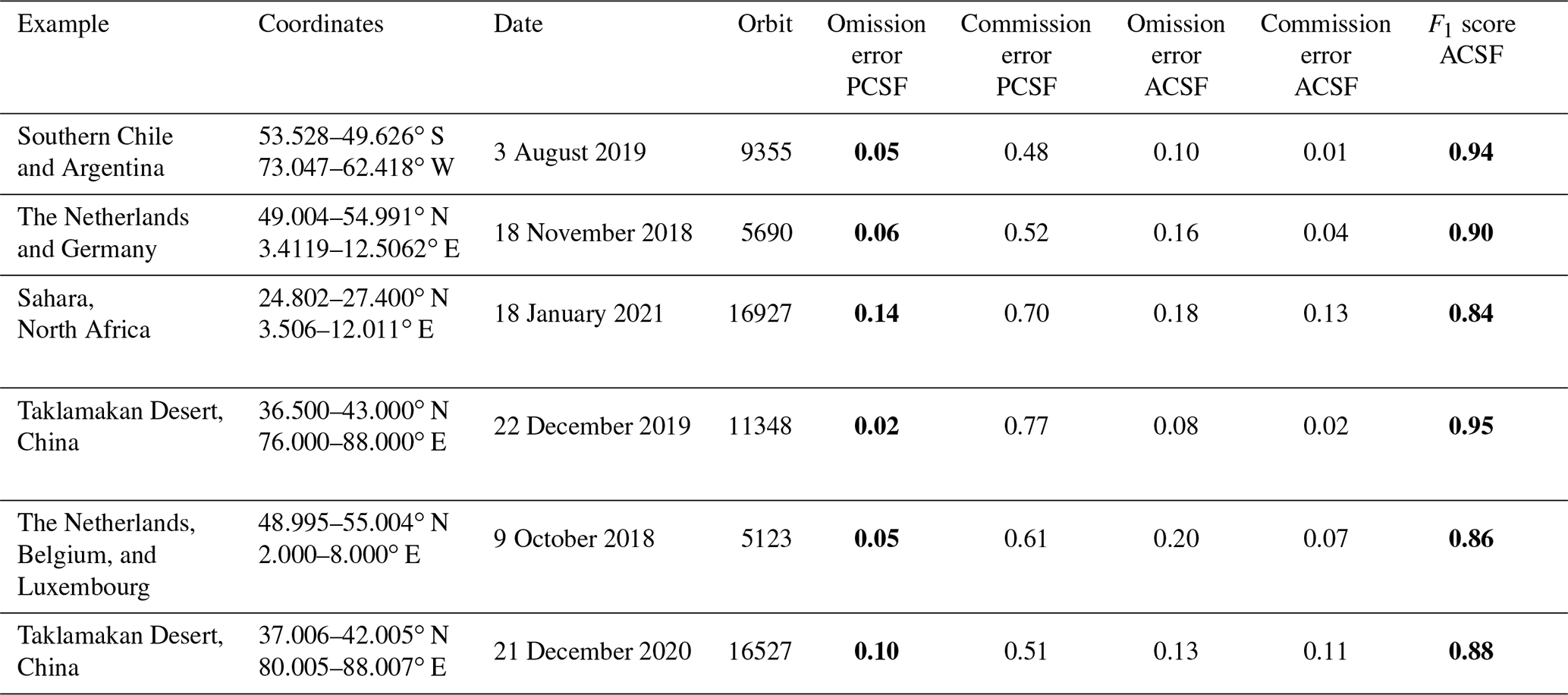
The fourth and fifth columns of Table 1 show ϵ_O and ϵ_C respectively of the PCSF. The value of ϵ_C of the PCSF is higher than 0.48 and higher than that of the ACSF, since the shadow in the PCSF is, by definition, an overestimation of the actual shadow. Because the PCSF is intended to be useful for excluding any cloud shadow contamination from TROPOMI Level 2 data, ϵ_O of the PCSF should be minimized. The value of ϵ_O for all examples is 0.14 or lower. Also here, we attribute the nonzero ϵ_O to the imperfect correction of the cloud movement during the TROPOMI–VIIRS measurement time difference and to thin and/or small clouds resulting in false negative CF. Again, the best performances are found for southern Chile and Argentina, 3 August 2019, and for the Taklamakan Desert, 22 December 2019, with an ϵ_O of 0.05 and 0.02 respectively.

In order to put the validation results in perspective, we note that the state-of-the-art imager cloud and cloud shadow detection code Fmask version 4.0 (Qiu et al., 2019) reports shadow detection commission errors of 0.49 for Landsat 4–7 and 0.38 for Landsat 8 and omission errors of 0.27 for Landsat 4–7 and 0.31 for Landsat 8. Using multi-temporal reference images of specific regions, Candra et al. (2019) achieved omission and commission errors ranging from 0.001 to 0.084 and 0 to 0.058 respectively, depending on the region. The PCSF omission errors and ACSF commission errors in Table 1 are lower than those of Fmask 4.0 and are of the same order of magnitude as those achieved by Candra et al. (2019). Of course, because of the much higher spatial resolution of Landsat than that of TROPOMI, the error values for Landsat actually refer to a much larger number of pixels.

5 Discussion

Here, we discuss some limitations and points of attention for the usage of the DARCLOS cloud shadow flags. Also, we point out the possible spectral dependence of cloud shadow extents and present the (unvalidated) spectral cloud shadow flag as an auxiliary product of DARCLOS.

5.1 Limitations of the ACSF and PCSF

The PCSF depends on the CF, which is determined by the effective cloud fraction. As discussed in Sect. 3.1, false negative cloud detections in the CF can result in falsely detected gaps in cloud decks, resulting in false positive PCSFs inside the gaps (Fig. 7a). Note that false negative cloud detections in the CF can also result in false negative shadow detections in the PCSF and ACSF, since there is no shadow to be detected in the absence of a cloud detection. The surface albedo input for the effective cloud fraction calculation in the NO₂ product is the LER climatology made by the Ozone Monitoring Instrument (OMI) at 440 nm available at a $\mathrm{0.5}{}^{\circ }\times \mathrm{0.5}{}^{\circ }$ latitude–longitude grid (Kleipool et al., 2008). With a future implementation of the TROPOMI DLER climatology, which uses a $\mathrm{0.125}{}^{\circ }\times \mathrm{0.125}{}^{\circ }$ latitude–longitude grid instead (see Sect. 2.2.2), in the effective cloud fraction algorithm, the accuracy of the CF, PCSF, and ACSF is expected to further increase.

DARCLOS has not been tested at regions covered by ice and/or snow, or at sunglint geometries over ocean. In these circumstances, the performance of the current effective cloud fraction is limited, often resulting in false positive CFs. For the ACSF, we have discarded the cloud pixels (and corresponding shadows) that contain a raised sunglint flag and/or snow/ice flag. For the PCSF, these pixels are not discarded, such that they are removed from the data when the PCSF and CF are used together to both remove cloud and cloud shadow contaminations. With future potential improvements of FRESCO above glint and snow/ice regions, DARCLOS could be tested above glint and snow/ice regions. Then, the DLER for snow/ice conditions (see Tilstra, 2022) should be employed in DARCLOS, and possibly an ocean surface reflectance calculation can help distinguish between clouds and then glint.

The performance of the ACSF depends on the quality of the DLER climatology. Although the DLER takes into account monthly surface reflectivity changes throughout the year, temporary deviations from this climatology (e.g. agricultural land usage changes, forest fires, precipitation, flooding, and snow cover) are measured by the SCNLER and may affect Γ and possibly the ACSF. In addition, the spatial resolution of the DLER of $\mathrm{0.125}{}^{\circ }\times \mathrm{0.125}{}^{\circ }$ is somewhat coarser than the spatial resolution of the TROPOMI Level 2 UVIS grid at which the SCNLER is measured. Dark small-scale surface features not captured by the DLER may, theoretically, give too low Γ and may result in false positive ACSF. In the examples treated in this paper, however, dark small-scale forest (Sect. 3.2) and desert (Sect. 3.3) features did not convincingly deteriorate the ACSF performance.

Both the irradiance and radiance measurements by TROPOMI have degraded during its operational lifetime. The irradiance measurements are known to degrade faster than the radiance measurements (and most significantly at the shortest wavelengths), leading to an increasing derived reflectance over time (Tilstra et al., 2020; Ludewig et al., 2020). Since the release of the version 2.0.0 TROPOMI level 1b processor on 5 July 2021, the irradiance degradation is being corrected. The thresholds used in this paper for clouds and cloud shadows, which were set at an effective cloud fraction of 0.05 and $\mathrm{\Gamma }=-\mathrm{15}$ % respectively, may have to be adjusted for the corrected data.

5.2 Spectral cloud shadow flag (SCSF)

In Sect. 4, the ACSF has been validated by visual inspection of true-colour images of the VIIRS instrument. Hence, the shadows found with the ACSF can be interpreted as the shadows that could be observed from space by the human eye. We find, however, a significant wavelength dependency of the contrast parameter Γ in the UV part of the spectrum. For example, Fig. 12a shows Γ at 340 nm for the example above the Netherlands and Germany on 18 November 2018. Comparing to Γ at λ_max (Fig. 8b), where λ_max=772 nm over land, the negative Γ related to cloud shadows between 52 and 53^∘ N latitude and 9 and 12^∘ E longitude have disappeared. Also, the locations of some pixels with significant negative Γ have changed. Although these shadows have not been validated (they could possibly not be observed by the human eye) or could be a result of noisy Γ in dark scenes (see Eq. 11), they may be relevant for studying shadow effects on TROPOMI air quality products retrieved at particular UV wavelengths, such as the absorbing aerosol index (AAI) at λ=340 nm and λ=380 nm (see de Graaf et al., 2005; Stein Zweers et al., 2018; Kooreman et al., 2020) or the NO₂ column at λ=440 nm (see van Geffen et al., 2021). Therefore, DARCLOS also outputs the spectral cloud shadow flag (SCSF), which is raised at PCSF pixels for which

$$\begin{array}{}\text{(17)}& \mathrm{\Gamma }\left(\mathit{\lambda }\right)<q,\end{array}$$

where q is again set at −15 %. Contrary to the ACSF (Eq. 13), the SCSF is by definition wavelength dependent. The SCSF is computed at 328, 335, 340, 354, 367, 380, 388, 402, 416, 425, 440, 463, and 494 nm.

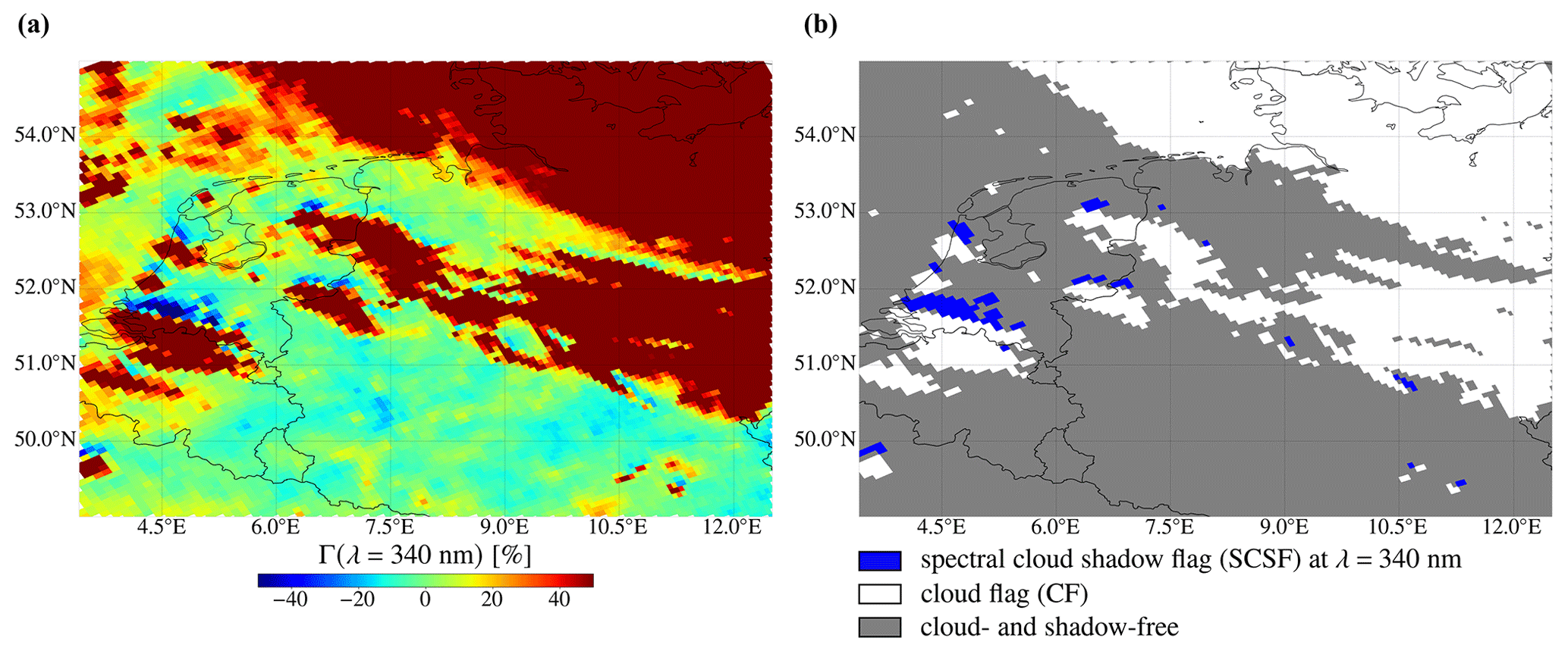
Figure 12 SCNLER–DLER contrast parameter Γ at λ=340 nm measured by TROPOMI (a) and TROPOMI Level 2 UVIS ground pixels with raised SCSFs at λ=340 nm (b), for the Netherlands and Germany on 18 November 2018. In (b), white pixels are cloud pixels, and grey pixels do not contain a raised cloud or shadow flag.

Figure 12b shows the SCSF at λ=340 nm for the example above the Netherlands and Germany on 18 November 2018. Comparing to Fig. 8d shows that part of the shadow flags have disappeared or have changed location. For example, the cloud shadow detected with the SCSF at $\sim \mathrm{49.5}{}^{\circ }$ N latitude and $\sim \mathrm{11.3}{}^{\circ }$ E longitude has shifted closer to the cloud compared to the corresponding ACSF shadow. We speculate that the wavelength dependence of shadow locations in the UV can be explained by the wavelength dependence of the molecular scattering optical thickness of the atmosphere: at shorter wavelengths, the molecular scattering optical thickness is higher such that higher atmospheric layers are probed from space, decreasing the observed shadow extents with TROPOMI. The explanation and validation of the wavelength dependence of observed cloud shadow extents in the UV are subject to future research.

6 Summary and conclusions

In this paper, we have demonstrated DARCLOS, a cloud shadow detection algorithm for TROPOMI. DARCLOS provides a potential cloud shadow flag (PCSF) based on geometric variables stored in TROPOMI Level 2 data and an actual cloud shadow flag (ACSF) based on the contrast of the measured scene reflectivity with the climatological surface reflectivity. For each TROPOMI pixel, this contrast is computed at the wavelength where the DLER is largest. The ACSFs are a subset of the PCSFs.

Three case studies with different spectral surface albedo and cloud types have been discussed in detail. We have shown that the PCSF vastly overestimates the shadows observed in true-colour images of the VIIRS-NPP instrument, as expected. The shadows detected with the ACSF are better approximations of these true shadows, but they may miss some shadows that are produced by thin and/or small clouds. We showed that the shadow signatures in the contrast between the scene reflectivity and the climatological surface reflectivity can, for almost all pixels, only be attributed to cloud shadows. That is, dark surface features are not falsely detected as cloud shadows in the ACSF.

The PCSF and ACSF are validated by visual inspection of true-colour images made by the VIIRS-NPP instrument for, in total, six cases. We found that the cloud motion during the measurement time difference between TROPOMI and VIIRS complicates this validation strategy. We showed that a cloud movement correction using the wind speed vectors at the cloud height significantly improves the validation results. The best detection scores were achieved for the cases with relatively thick and horizontally large cloud decks (ACSF F₁ score ≥0.94 and PCSF omission error ≤0.05). After the cloud movement correction, the validation may still suffer from cloud evolution and the relatively coarse resolution of the wind product. Hence, the true shadow detection performance at the TROPOMI measurement times may be expected to be even better than presented with the validation in this paper.

At UV wavelengths, we have found cloud shadow signatures at different locations than determined with the ACSF, potentially indicating a wavelength-dependence of cloud shadow extents. Because TROPOMI's air quality products are retrieved at specific wavelengths or wavelength ranges, DARCLOS also outputs the spectral cloud shadow flag (SCSF), which is a wavelength dependent alternative for the ACSF. Such a cloud shadow detection at the precise wavelengths of TROPOMI's air quality products is unique for DARCLOS and cannot be done with data from an imager.

The shadow flags of DARCLOS are planned for implementation in the TROPOMI L2 SCNLER product. DARCLOS is, to the best of our knowledge, the first cloud shadow detection algorithm for a spaceborne spectrometer instrument. In principle, DARCLOS can also be used for other spectrometer instruments than TROPOMI which have a spatial resolution high enough to observe cloud shadows. An effective cloud fraction and climatological surface albedo are prerequisites for DARCLOS and should therefore be available at the ground pixel grid of the instrument. It should be noted that, when computing the ACSF using UVIS and NIR wavelengths from different detectors, a co-registration of the SCNLER measurements from one detector ground pixel grid to the other has to be performed. Ideally, true-colour images are available of the scenes with approximately the same measurement times, in order to validate the PCSF and ACSF by visual inspection and to optimize the cloud and cloud shadow thresholds.

We conclude that the PCSF can be used to remove cloud-shadow-contaminated pixels from TROPOMI Level 2 UVIS data, and that the ACSF can be used to select pixels for further analysis of cloud shadow effects. If both cloud and cloud shadow effects are to be removed, the PCSF and CF can be used together. Also, the ACSF can be used to demonstrate and/or count the true shadows that would be observed from space by the human eye. However, at UV wavelengths, we have found indications of the wavelength dependence of cloud shadow signatures, and a spectrally dependent cloud shadow flag such as the SCSF could possibly be more suitable when selecting shadow pixels in air quality products retrieved at UV wavelengths. Further research is needed to explain and validate the spectral dependence of these cloud shadow signatures. The detection of shadows with the ACSF and SCSF allows users to perform this analysis and is a first step towards the understanding and correction of cloud shadow effects on satellite spectrometer air quality measurements.