the Creative Commons Attribution 4.0 License.
the Creative Commons Attribution 4.0 License.
 | 20 May 2022
Measurement of the vertical atmospheric density profile from the X-ray Earth occultation of the Crab Nebula with Insight-HXMT
Daochun Yu
Haitao Li
Baoquan Li
Mingyu Ge
Youli Tuo
Xiaobo Li
Wangchen Xue
Yaning Liu
Aoying Wang
Yajun Zhu
Bingxian Luo
X-ray Earth occultation sounding (XEOS) is an emerging method for measuring the neutral density in the lower thermosphere. In this paper, the X-ray Earth occultation (XEO) of the Crab Nebula is investigated using the Hard X-ray Modulation Telescope (Insight-HXMT). The pointing observation data on the 30 September 2018 recorded by the low-energy X-ray telescope (LE) of Insight-HXMT are selected and analysed. The extinction light curves and spectra during the X-ray Earth occultation process are extracted. A forward model for the XEO light curve is established, and the theoretical observational signal for light curve is predicted. The atmospheric density model is built with a scale factor to the commonly used Mass Spectrometer Incoherent Scatter Radar Extended model (MSIS) density profile within a certain altitude range. A Bayesian data analysis method is developed for the XEO light curve modelling and the atmospheric density retrieval. The posterior probability distribution of the model parameters is derived through the Markov chain–Monte Carlo (MCMC) algorithm with the NRLMSISE-00 model and the NRLMSIS 2.0 model as basis functions, and the respective best-fit density profiles are retrieved. It is found that in the altitude range of 105–200 km, the retrieved density profile is 88.8 % of the density of NRLMSISE-00 and 109.7 % of the density of NRLMSIS 2.0 by fitting the light curve in the energy range of 1.0–2.5 keV based on the XEOS method. In the altitude range of 95–125 km, the retrieved density profile is 81.0 % of the density of NRLMSISE-00 and 92.3 % of the density of NRLMSIS 2.0 by fitting the light curve in the energy range of 2.5–6.0 keV based on the XEOS method. In the altitude range of 85–110 km, the retrieved density profile is 87.7 % of the density of NRLMSISE-00 and 101.4 % of the density of NRLMSIS 2.0 by fitting the light curve in the energy range of 6.0–10.0 keV based on the XEOS method. Goodness-of-fit testing is carried out for the validation of the results. The measurements of density profiles are compared to the NRLMSISE-00 and NRLMSIS 2.0 model simulations and the previous retrieval results with NASA's Rossi X-ray Timing Explorer (RXTE) satellite. For further confirmation, we also compare the measured density profile to the ones by a standard spectrum retrieval method with an iterative inversion technique. Finally, we find that the retrieved density profile from Insight-HXMT based on the NRLMSISE-00 and NRLMSIS 2.0 models is qualitatively consistent with the previous retrieved results from RXTE. The results of light curve fitting and standard energy spectrum fitting are in good agreement. This research provides a method for the evaluation of the density profiles from MSIS model predictions. This study demonstrates that the XEOS from the X-ray astronomical satellite Insight-HXMT can provide an approach for the study of the upper atmosphere. The Insight-HXMT satellite can join the family of the XEOS. The Insight-HXMT satellite with other X-ray astronomical satellites in orbit can form a space observation network for XEOS in the future.
- Article
(6252 KB) - Full-text XML
- BibTeX
- EndNote


The middle and upper atmosphere is affected by both solar activity and geomagnetic disturbance, so it is of great significance to study the density of the middle and upper atmosphere for further understanding solar–terrestrial relationships (Rhoden et al., 2000; Prölss, 2011). The middle and upper atmosphere is the passage area of re-entry vehicles. In addition, the middle and upper atmosphere density is extremely important as an input of aerodynamic force and heating design of re-entry vehicles (Riley and Dejarnette, 1992; Davis and White, 2008), although it is very thin. In addition, manoeuver planning, precise orbit determination and satellite lifetime predictions are limited by the accuracy of neutral density in the thermosphere (Doornbos and Klinkrad, 2006; Kalafatoglu Eyiguler et al., 2019).
However, the measured data of the density in the middle and upper atmosphere are scarce, especially in the upper mesosphere and lower thermosphere (60–200 km), due to the limitation of detection methods (Russell et al., 1999; Baron et al., 2020; Zeitler et al., 2021). With the increasing demand for the density of the Earth's middle and upper atmosphere, various semi-empirical atmosphere models have been developed, such as the Jacchia Reference Atmosphere (Jacchia, 1970, 1977), the Drag Temperature Model (DTM) (Berger et al., 1998; Bruinsma et al., 2003) and the Mass Spectrometer Incoherent Scatter Radar Extended model (MSIS) (Hedin, 1987; Picone et al., 2002) from the Naval Research Laboratory. Generally, there are still errors of around 30 % rms and peak errors of 100 % or more in these semi-empirical models due to the complex changes in the middle and upper atmosphere (Doornbos et al., 2008). Some new methods have been developed to detect the density of the Earth's middle and upper atmosphere.
Originally, in situ measurements were used to obtain the density of the middle and upper atmosphere, which is a way to obtain the atmosphere density directly by payloads from sounding rockets. In situ measurements of atmospheric density near orbit can be achieved by using satellites. As an in situ measurement method, falling sphere measurements can also provide the vertical atmospheric density profiles (Bartman et al., 1956; Faire and Champion, 1965; Faucher et al., 1967; Haycock et al., 1968). The nitric oxide density profile between 60 and 96 km was deduced from measurements by a sounding rocket (Pearce, 1969). The local-noon mean ozone distribution was obtained by analysing the data from 21 sounding rockets carrying the Arcas optical ozonesondes up to 52 km (Krueger, 1973). Direct measurements of atmospheric density at high altitudes, especially above 100 km, using sounding rocket methods are difficult because of the short duration of rocket flights and their high cost (Watanabe, 1958). China completed the atmospheric density detection and precise orbit determination (APOD) mission with four CubeSats, which was designed to estimate atmospheric density below 520 km using in situ sounding and precision orbit products and to demonstrate the link between geomagnetic storms and density enhancements (Tang et al., 2020). In order to obtain the spatiotemporal variation characteristics of atmospheric density on a global scale, the remote sensing by satellites is gradually developed. As a scientific instrument of Thermosphere Ionosphere Mesosphere Energetics and Dynamics (TIMED) that is the initial mission under NASA's Solar Terrestrial Probes programme, Sounding of the Atmosphere Using Broadband Emission Radiometry (SABER) can obtain vertical profiles of several atmospheric constituents, such as O3, H2O, and CO2, as well as neutral atmospheric density in the altitude range of ∼10–140 km (Russell et al., 1999; Meier et al., 2015; Rezac et al., 2015).
In addition to the direct measurements of atmospheric density by sounding rockets, satellites, and falling sphere measurements, retrieval of atmospheric density can also be carried out by an indirect method that usually refers to the method of occultation sounding. Stellar occultation has a long history as an atmospheric diagnostic method. The technique of retrieval of atmospheric density by occultation has gradually been developed. There are some previous studies on the retrieval of atmospheric density of specific species by stellar occultation in the ultraviolet band. Hays and Roble (1973) obtained the night-time vertical distribution of ozone number density in an altitude range of 60–100 km at low latitudes by analysing the results of approximately 12 stellar occultations in the ultraviolet band near 2500 Å. Aikin et al. (1993) measured the molecular oxygen densities in the altitude range of 140–220 km based on the solar occultation data obtained from the ultraviolet spectrometer/polarimeter (UVSP) on the Solar Maximum Mission (SMM) spacecraft. The density profiles of ozone and nitrogen dioxide were inverted and evaluated by an optimal estimation algorithm using solar occultation data from SCanning Imaging Absorption spectroMeter for Atmospheric CHartographY (SCIAMACHY) in the UV–Vis wavelength range (Meyer et al., 2005). Lumpe et al. (2007) used an optimal estimation algorithm to obtain the O2 density profiles between 110 and 240 km by analysing solar occultation data at three nominal wavelengths (144, 161, and 171 nm). In addition to relevant studies in the ultraviolet band, occultation in the infrared and radio band has also been extensively studied. The water vapour number density profiles in the altitude range of 15–45 km were retrieved from the solar occultation data by SCIAMACHY in the wavelength region around 940 nm (Noël et al., 2010). The radio occultation technique can often be used to retrieve the electron density in the ionospheric by the Abel integral equations (Hajj and Romans, 1998; Lei et al., 2007; Chou et al., 2017). There are also occultation measurements that retrieve atmospheric density for specific species, such as SOFIE/AIM (McHugh et al., 2008; Rong et al., 2016), GOMOS/Envisat (Renard et al., 2008; Kyrölä et al., 2010), SAGE series (Degenstein et al., 2018; McCormick et al., 2020), and POAM series (Rusch et al., 2001; Lumpe et al., 2002).
The study of the atmosphere by X-ray occultation is a new interdisciplinary study. The atmospheric extent of Titan was measured by the transit of the Crab Nebula in the X-ray band on 5 January 2003, observed by the Chandra X-Ray Observatory (Mori et al., 2004). Rahmati et al. (2020) obtained the neutral density of the atmosphere of Mars in the altitude range of 50–100 km by the Martian atmosphere occultation of 10 keV Scorpius X–1 X-rays using the SEP instrument on the MAVEN satellite. The X-ray Earth occultation technique is also a unique method to retrieve the neutral atmospheric density in the upper mesosphere and lower thermosphere. Based on the X-ray occultation of the Crab Nebula with ARGOS/USA and the X-ray occultation of Cygnus X–2 with RXTE/PCA, Determan et al. (2007) obtained the Earth's atmospheric density in the altitude ranges of 100–120 km and 70–90 km. Very recently, the Earth's average atmospheric density at low latitudes in the altitude range of 70–200 km was measured by analysing 219 X-ray Earth occultation data of the Crab Nebula with Suzaku and Hitomi (Katsuda et al., 2021). However, the retrieved atmospheric densities are significantly lower than the model density in some altitude ranges, and the difference between the measured values and the model values may result from the long-term accumulation of greenhouse gases, imperfect climatological estimates of solar and geomagnetic effects, temperature profile differences, or gravity waves (Determan et al., 2007; Katsuda et al., 2021). Therefore, it is very important to cross-check the density structure of Earth's atmosphere using observations from other X-ray satellites like Insight-HXMT, to further verify the difference between retrieved results and model density.
X-ray Earth occultation sounding (XEOS) has many advantages as an atmospheric diagnostic method. X-ray photons are absorbed directly by the K-shell and L-shell electrons of atoms, including atoms within molecules, in the extinction process. Therefore, the ionized states, electronic states, and chemical bonds within the molecules of atmospheric components have no effect on the absorption of X-rays. XEOS can retrieve the neutral atmospheric density in the upper mesosphere and lower thermosphere. In addition, the global distribution of the neutral atmosphere in the upper mesosphere and lower thermosphere can be obtained by analysing a large number of X-ray Earth occultation data from X-ray satellites, and the temporal evolution characteristics of neutral atmosphere density in this altitude range can also be studied. In this work, we use Insight-HXMT observational data to study the X-ray Earth occultation of the Crab Nebula in order to demonstrate the capability of Insight-HXMT as an atmospheric diagnostic instrument. In addition, the retrieved results of Insight-HXMT and RXTE are used to cross-check the density structure of Earth's atmosphere, so as to confirm the existence of differences between retrieved results and model values. Here, the theoretical model of the light curve is established by simulating the observations of the low-energy X-ray telescope (LE) (Chen et al., 2020) to the Earth occultation of the Crab Nebula. A Bayesian data analysis framework is developed for the XEO light curve modelling and the atmospheric density retrieval. We use the Markov chain–Monte Carlo (MCMC) algorithm to calculate the posterior probability distribution of model parameters, which is a method of inverting model parameters using Bayesian inference (Sharma, 2017). Finally, the Earth's atmospheric density in the altitude range of 85–200 km is retrieved.
The paper is structured as follows. Section 2 describes the observations and data reduction. Section 3 shows light curve modelling and density profile retrieval. The conclusions and discussions are given in Sect. 4.
Insight-HXMT is the first X-ray astronomy satellite in China (Zhang et al., 2018, 2020; Li et al., 2018). It is designed for several main scientific objectives, including the monitoring and studying of galactic plane scanning, X-ray binary observation, gamma-ray bursts, and gravitational wave electromagnetic counterparts (Zhang et al., 2020). The Insight-HXMT mainly carries four scientific payloads, including the high-energy x-ray telescope (HE), the medium-energy X-ray telescope (ME), the low-energy X-ray telescope (LE), and the Space Environment Monitor (SEM) (Zhang et al., 2018, 2020). The quality of calibration directly determines the achievement of the three main scientific objectives. The Crab Nebula is one of the brightest X-ray sources in the sky, with its stable evolution and brightness. Therefore, the Crab Nebula is an excellent calibration source for many X-ray satellites. The Crab Nebula as a standard candle has been widely used for in-flight calibration of space missions in X-ray astronomy (Kirsch et al., 2005; Meyer et al., 2010). In this work, the Crab Nebula is chosen as our observation source. The pointed observation mode is selected for the study of the X-ray Earth occultation.
2.1 Observation geometry
As Crab Nebula sets behind or rises from the limb of Earth as seen by Insight-HXMT, the X-ray flux from the Crab Nebula detected by Insight-HXMT varies due to the absorption of X-ray photons by Earth's atmosphere. The observation geometry of the X-ray Earth occultation of the Crab Nebula with Insight-HXMT is shown in Fig. 1. In the process of the X-ray Earth occultation, the atmosphere reduces the flux of the X-rays detected by Insight-HXMT. As the line of sight moves closer to the Earth's surface (setting), more X-ray photons are absorbed by the atmosphere, and vice versa.
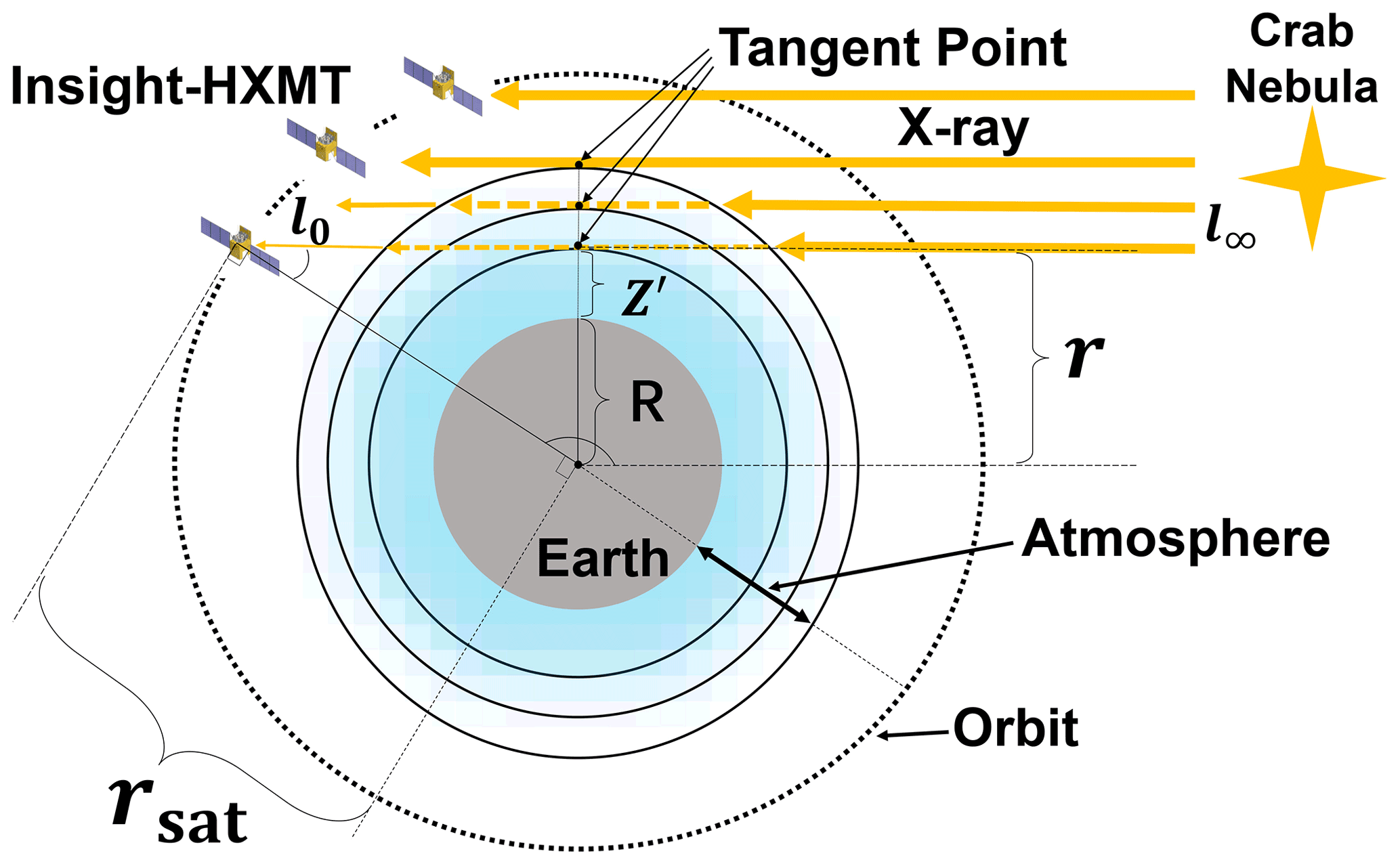
Figure 1The observation geometry of the X-ray Earth occultation of the Crab Nebula with Insight-HXMT. Tangent point altitude (Z′) is the shortest distance from the Earth's surface to the line of sight. The line of sight is defined as the line from the satellite position l0 to the X-ray source position l∞. rsat is the distance from the satellite to the centre of the Earth. r is the distance from the tangent point to the centre of the Earth. R is the radius of the Earth. The dotted line shows the satellite orbit. The extent of the atmosphere is marked by a double-sided arrow. The location of the tangent point is marked. The Insight-HXMT and the Crab Nebula are also marked. For clarity, only three layers of the atmosphere are marked, as shown by the solid black lines. The thick, solid orange lines with arrows show the X-rays before absorption and scattering. The dashed orange lines with arrows show the absorption and scattering of X-rays by the atmosphere. The thin, solid orange lines with arrows show X-rays passing through the atmosphere.
2.2 Data reduction
The observation data of the low-energy X-ray telescope (LE) are used in this study. We select the photons observed by detectors for LE because the extinction effect at a lower energy band during the occultation is obvious due to the larger cross section of the Earth's upper atmospheric compositions (Fig. 2). LE consists of three detector boxes each containing 32 pieces of CCD236 (Chen et al., 2020), which is the second-generation swept charge device (SCD) designed for X-ray spectroscopy (Holland and Pool, 2008; Zhao et al., 2019). The collimators divide each detector box of LE into four kinds of fields of view (FOV). For each detector box, 20 CCD236 devices have small FOVs of 1.6∘ × 6∘, 6 CCD236 devices have wide FOVs of 4∘ × 6∘, 2 CCD236 devices are blind FOVs, and 4 CCD236 devices have large FOVs of about 50–60∘ × 2–6∘ (Zhao et al., 2019; Chen et al., 2020; Zhang et al., 2020). The detector response matrix is generated through the calibration database hxmt CALDB (v2.05) (http://hxmtweb.ihep.ac.cn/caldb/628.jhtml, last access: 7 May 2022). Only observations from the small FOV detectors, excluding the detectors with ID 29 and 87 that are damaged, are used for analysis in order to get an accurate background in this paper.
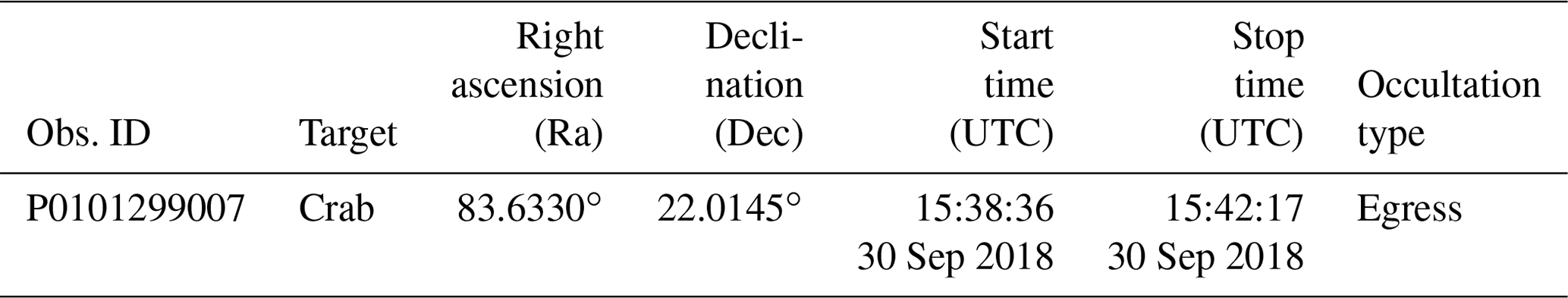
The information of the observation data selected in the data reduction is listed in Table 1, including the observation ID, the start and end time of the observation, the target source, and the right ascension and declination of the source in the coordinate system J2000. In the data reduction process, using HXMTsoft(v2.04) (http://hxmtweb.ihep.ac.cn/software.jhtml, last access: 7 May 2022), we extract the light curves and spectra of the Crab Nebula during Earth occultation recorded with LE. For the LE instrument, the photon counts are recorded by CCD236 detectors. Since we mainly study the occultation process of the Crab Nebula by the Earth atmosphere, the good time interval is screened by the following criteria: ELV (the elevation of the pointing direction above the horizon) less than 10∘.

Figure 2X-ray cross sections for Ar, O, and N. The energy ranges of LE, ME, and HE are indicated by shaded areas in light blue, light red, and light green to better distinguish the cross sections of each energy range. LE, ME, HE, and their respective energy ranges are also marked by bidirectional arrows. The calibrated energy range of LE is shown. A barn is a unit of area where 1 barn = 1 cm−24.
Table 1Summary of X-ray Earth occultation of the Crab Nebula analysed in this study.
2.3 Description of spectra and light curves
The comparison of the X-ray energy spectra during the occultation process is shown in Fig. 3. Five X-ray spectra in different altitude ranges are shown for clarity. These five energy spectra in blue, red, orange, magenta, and green in Fig. 3 are derived from the results of subsamples at altitudes of 160–170, 120–130, 100–110, 90–100, and below 70 km, starting from an unattenuated energy spectrum to the partially attenuated energy spectrum and ending with a fully attenuated energy spectrum. It is shown that the flux of the X-ray energy spectrum attenuates with reducing tangent point altitude during the occultation. Moreover, the absorption of X-ray photons by the atmosphere decreases with increasing energy.
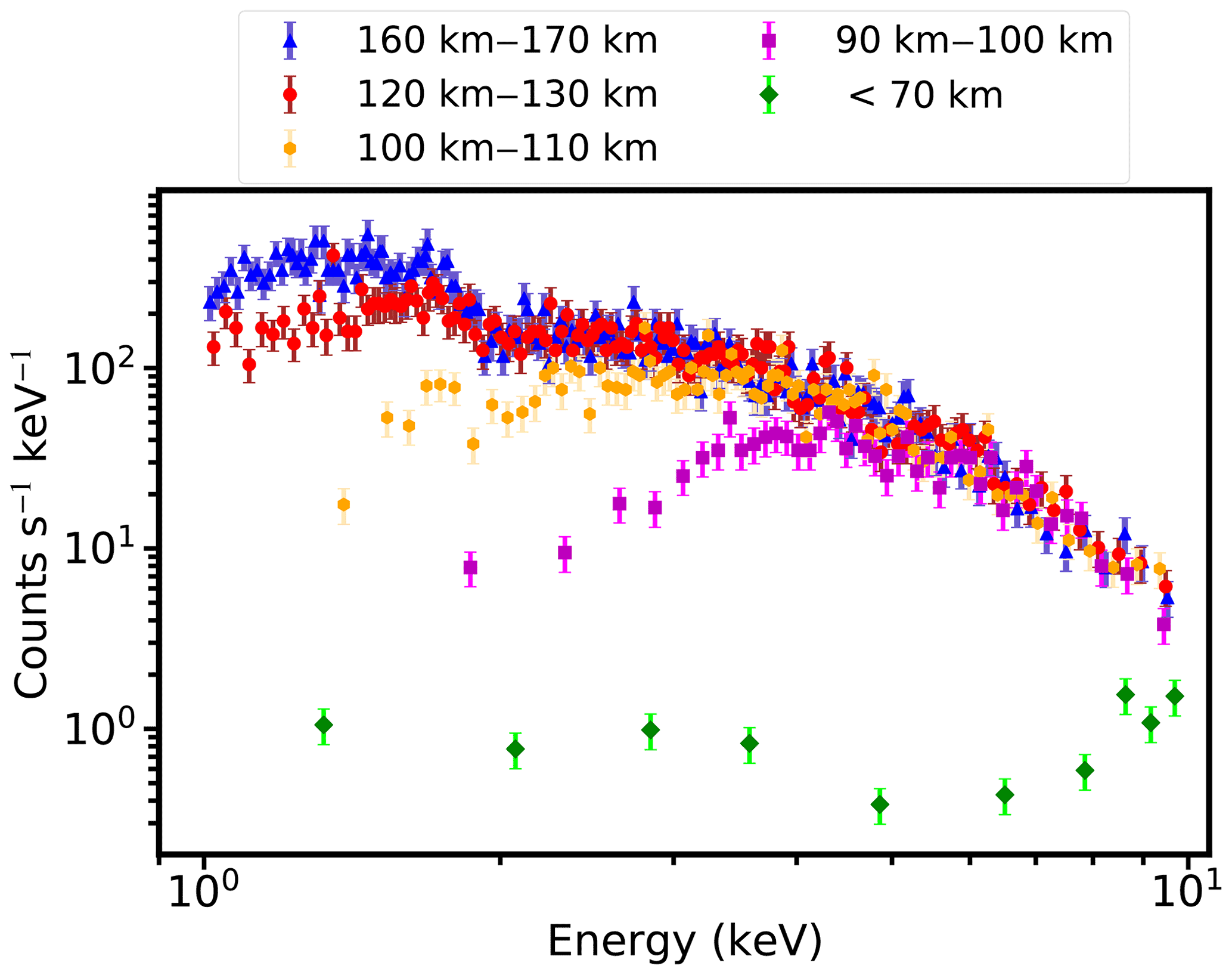
Figure 3The comparison of the X-ray energy spectra during the occultation process. These spectra cover an energy range of 1–10 keV (0.1240–1.2398 nm). The unattenuated X-ray energy spectrum is shown in blue. The red, orange, and purple data points are the attenuated X-ray energy spectra with the decreasing tangent point, respectively. The energy spectrum in green is the fully attenuated X-ray spectrum.
In the process of X-ray Earth occultation of the Crab Nebula, the Crab Nebula and Earth's atmospheric disks are tangent at four contact times tI−tIV, illustrated in Fig. 4. The total duration is , the full duration is , the ingress duration is , and the egress duration is . The occultation depth δ is the X-ray flux attenuation due to the extinction.
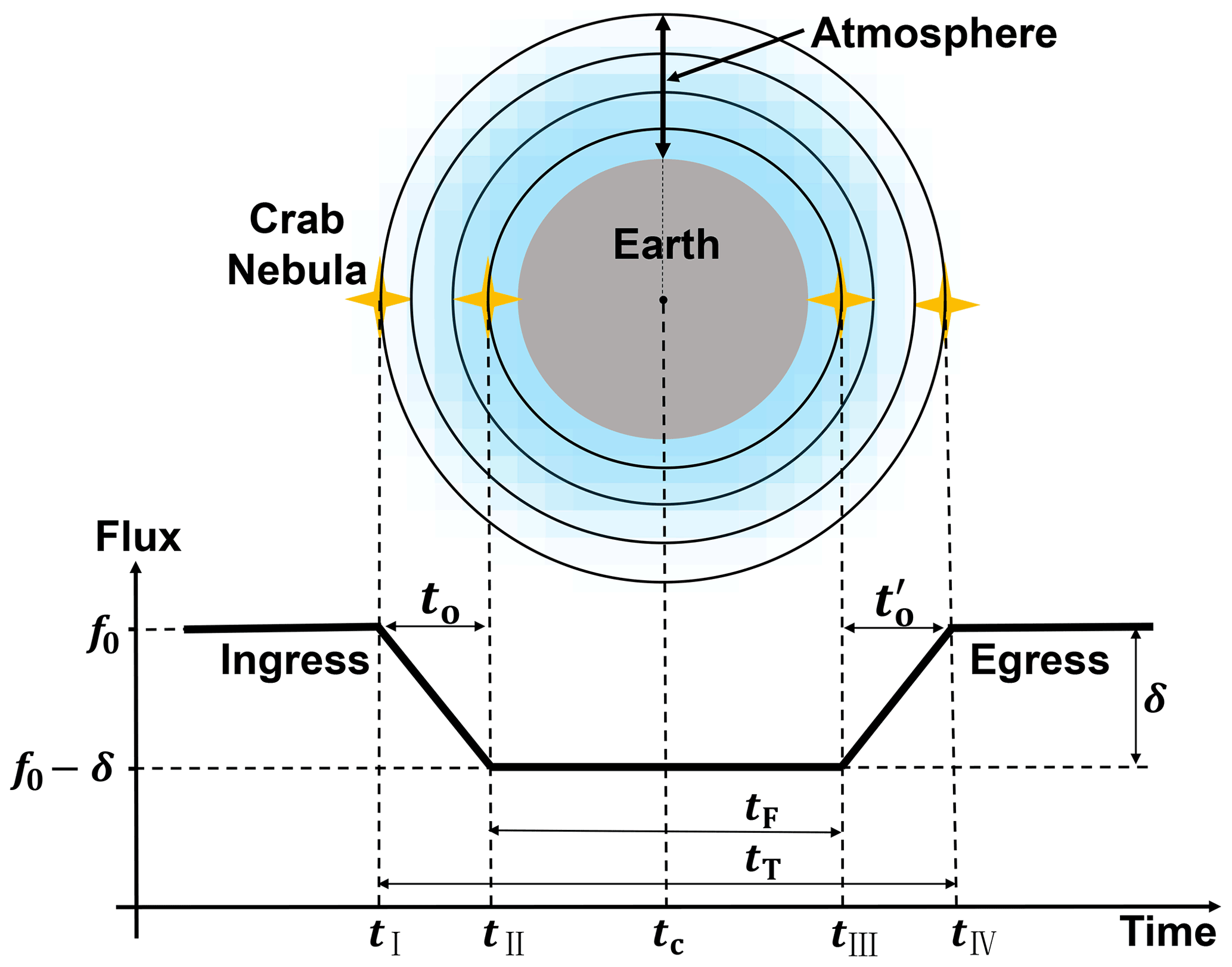
Figure 4Illustration of an X-ray Earth occultation of the Crab Nebula, showing the light curve discussed in Sect. 2.2, the four contact points tI, tII, tIII, and tIV, and the quantities to, tF, t T, tc, and δ defined in Sect. 2.3. As a low-earth orbit (LEO) satellite, Insight-HXMT can observe the Crab Nebula twice in one orbit (egress and ingress). The length of tF is half the orbital period minus the duration of two occultations, and the orbital period of Insight-HXMT is about 96 min.
The egress duration is about 14 s during the occultation process analysed in this study. We divide this duration into 35 bins in order to have good time resolutions and a high signal-to-noise ratio (SNR). The light curves of three different energy bands during the occultation process are shown in Fig. 5. The abscissa time is converted to tangent point altitude. In this study, the maximum height difference between two adjacent tangent points is 836 m, and the mean height difference between two adjacent tangent points is about 673 m. For clarity, the data points in Fig. 5 are displayed by taking 1 point every 10 points from the initial data points. The dashed blue, red, and green lines represent the modelled light curves. The green and blue shaded regions correspond to the extinction process for the occultation in the energy bands of 1.319–1.725 and 7.006–7.412 keV, respectively. For clarity, the height range for occultation between 3.350 and 3.756 keV is not marked. The light curve in the energy range of 1.319–1.725 keV starts to attenuate at 150 km, and it is completely attenuated at 102 km. The light curve in the energy range 7.006–7.412 keV starts to attenuate at 100 km, and it is completely attenuated at 85 km.
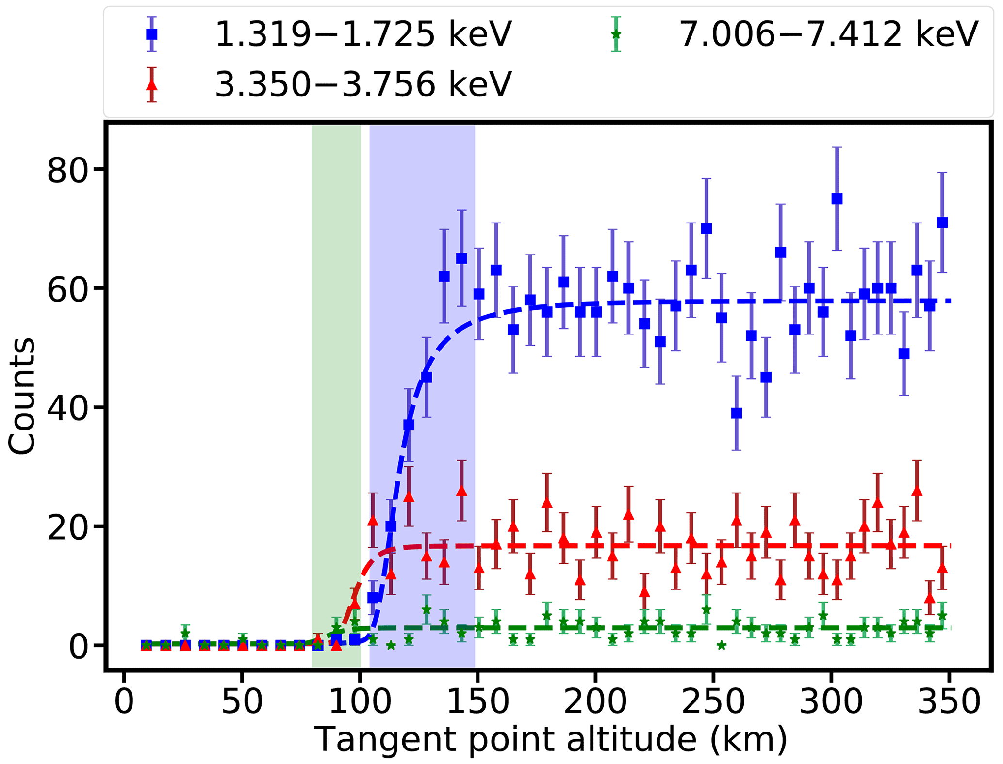
Figure 5The light curves during the occultation process. The points with the error bars are observation data. The dashed blue, red, and green lines represent the modelled light curves. The green shaded region corresponds to the height range for the occultation in the energy bands of 7.006–7.412 keV. The height range for occultation in the energy range of 7.006–7.412 keV is about 85–100 km. The blue shaded region corresponds to the height range for the occultation in the energy bands of 1.319–1.725 keV. The height range for occultation in the energy range of 1.319–1.725 keV is about 102–150 km. For clarity, the height range for occultation between 3.350 and 3.756 keV is not marked. The height range for occultation in the energy range of 3.350–3.756 keV is about 90–110 km. The reason for the relatively large variability of each light curve is the absorption of X-ray photons by atoms of atmospheric constituents.
In this section, we will describe the details of the light curve modelling for the X-ray Earth occultation of the Crab Nebula. In this study, we model the Earth occultation as a measurement method for atmospheric density.
X-rays can be absorbed by the photoelectric effect. The ionized states, electronic states, and chemical bonds within the molecules of atmospheric components have no effect on the absorption of X-rays in the extinction process. X-ray photons are absorbed directly by the K-shell and L-shell electrons of atoms, including atoms within molecules. Therefore, the X-ray Earth occultation can work as an atmospheric diagnostics method. In this case, the source celestial coordinates and the satellite positions are known, whereupon the atmospheric density profile can be treated as the unknown. It is impossible to distinguish atoms from molecules (in the calculation process), although X-ray photons interact directly with the K- and L- shell electrons of atoms (including atoms within molecules). The O2 (or N2) counts as one absorbing “particle” in the calculation, so the total neutral atmospheric density profile can be retrieved by X-ray occultations (Katsuda et al., 2021).
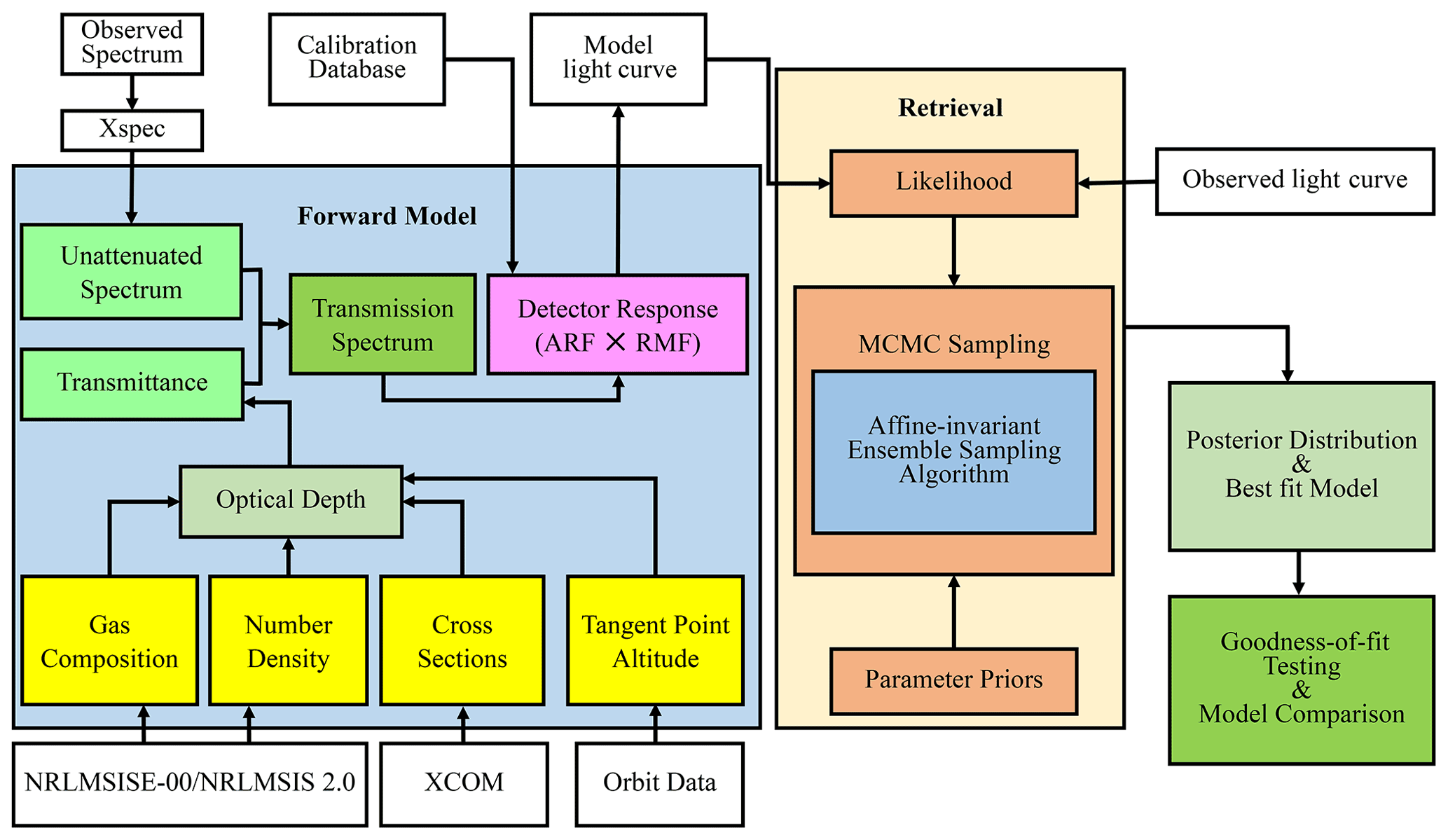
The schematic of light curve modelling of the X-ray Earth occultation is shown in Fig. 6. The attenuation process of the X-ray energy spectrum can be described by the Beer–Lambert law during the occultation. The attenuation energy spectrum is convolved with the detector response matrix to obtain the forward model. Given the data and the forward model, Bayesian inference is used to estimate the model parameters. Given the prior distribution and the likelihood function, the posterior probability distribution of the model parameters is calculated by MCMC. The best-fit model is obtained from the posterior probability distribution of the model parameters. The results will be compared with other measurements and models. The details of the data analysis will be described in the following subsection.
3.1 Forward model
The attenuation process of X-rays in the atmosphere can be described by the Beer–Lambert law:
where I0 is the unattenuated source spectrum, which is a function of energy, e−τ is the transmittance, and τ is the optical depth, which has the form
where s labels the gas components in the Earth's atmosphere, γ is the total correction factor, and ns is the number density of each component of the atmosphere along the line of sight. Based on the spherical symmetry assumption of the Earth atmosphere, the number density is converted to column density by the Abel integral. σs is the X-ray cross section (photoelectric absorption and scattering cross section) of each component in the atmosphere. X-ray photons are absorbed or scattered by atoms, and in the energy range of interest in this paper, the scattering effect can be ignored because it is too small relative to the photoelectric absorption effect. However, the scattering cross section is still included in the calculation.
The modelled light curves with this forward model are shown in Fig. 7 from Insight-HXMT for the X-ray Earth occultation of the Crab Nebula. The normalized flux with the orbital phase is shown. From Fig. 7, we can see that the occultation depths (the difference between the highest and lowest point of the same light curve) for different energy bands are very different. Here, the atmospheric model NRLMSISE-00 (Picone et al., 2002) is chosen as our input data in the light curve calculations in Fig. 7.
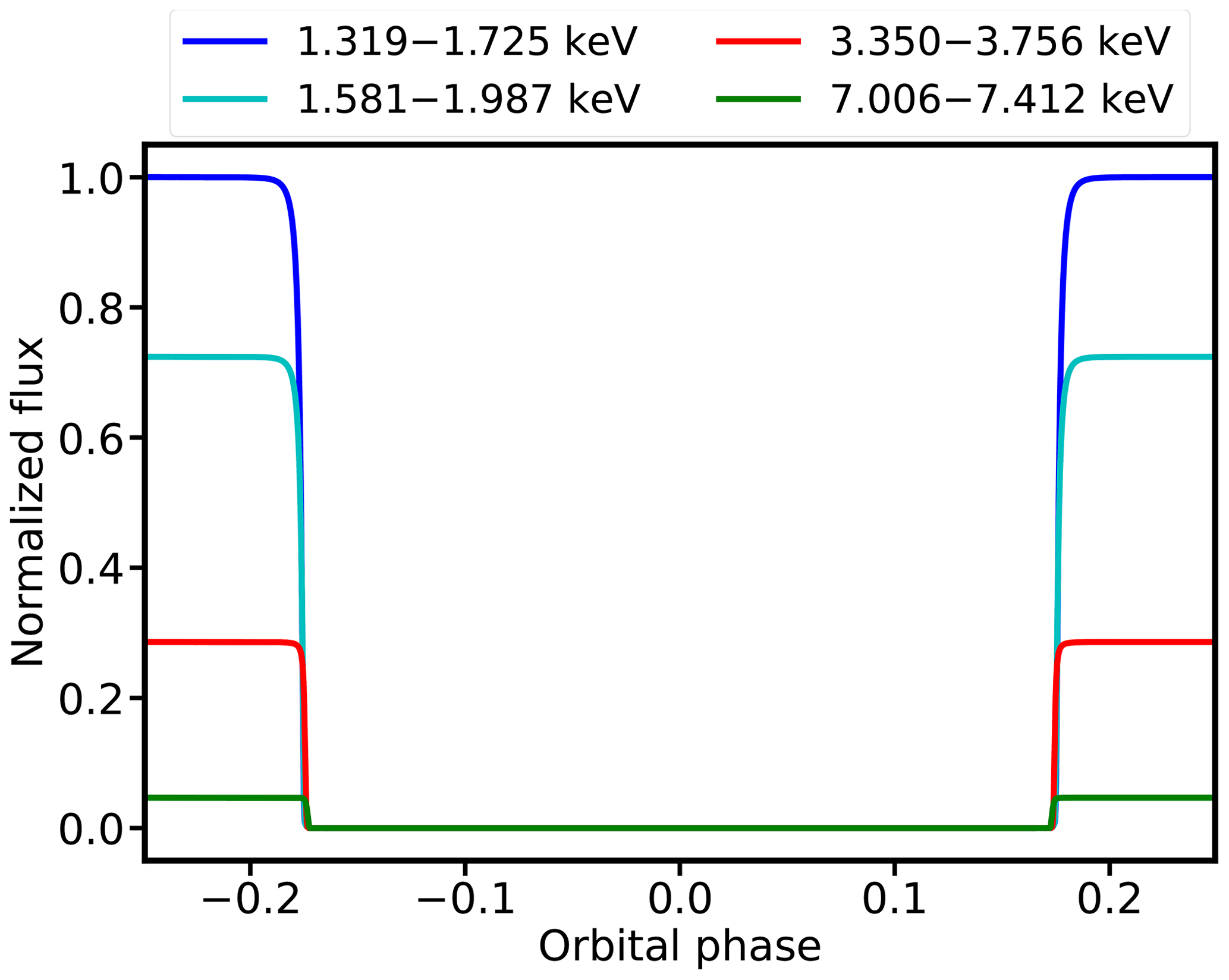
Figure 7The modelled light curves from Insight-HXMT for the X-ray Earth occultation of the Crab Nebula. The blue, cyan, red, and green predicted light curves correspond to four different energy ranges, and these predicted light curves are all calculated based on the input data from the NRLMSISE-00 model. The normalized flux of each predicted light curve is represented with the orbital phase. It is found that the occultation depths (the difference between the highest and lowest point of the same light curve) of different energy segments are very different.
I0 was fitted by using Xspec, a standard software package for spectrum fitting in X-ray astronomy. To fit the unattenuated spectrum of the Crab Nebula, we use the model wabs × powerlaw (Godet et al., 2009; Yan et al., 2018), where “wabs” is the interstellar absorption model in Xspec (Morrison and McCammon, 1983; Arnaud et al., 1999). The model “powerlaw” represents a simple power law shape of spectrum to fit. The data description and fitting result of unattenuated energy spectrum are listed in Table 2. The reduced χ2 value (Mighell, 1999) is 1.06 in this fitting, which indicates that the fit is good. The best-fit model and the unattenuated energy spectrum data are shown in Fig. 8a. The blue dots with the error bars are the unattenuated spectrum of the Crab Nebula observed by LE. The solid red line is the best-fit model. Figure 8b shows the residuals of the fit.
Table 2Data description and fitting results of the unattenuated energy spectrum.
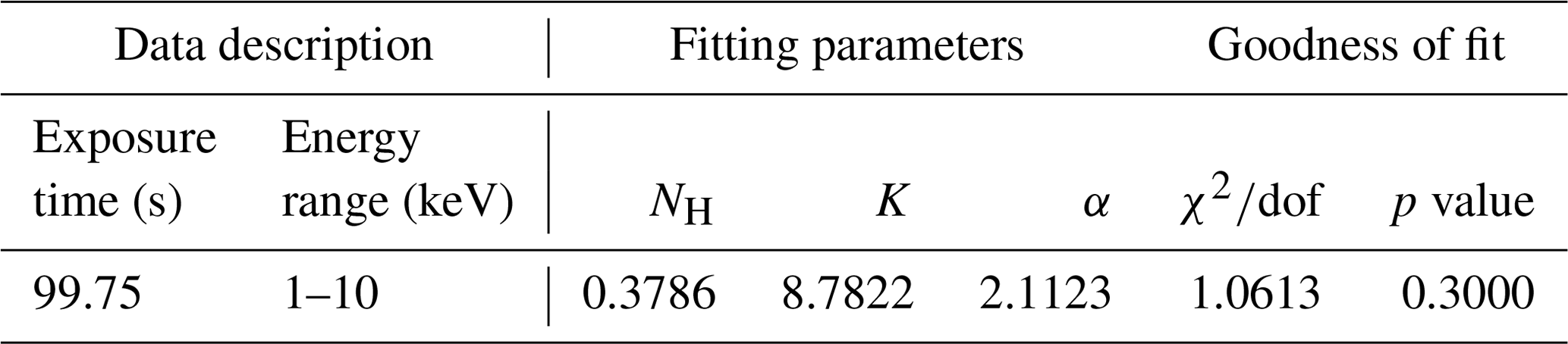
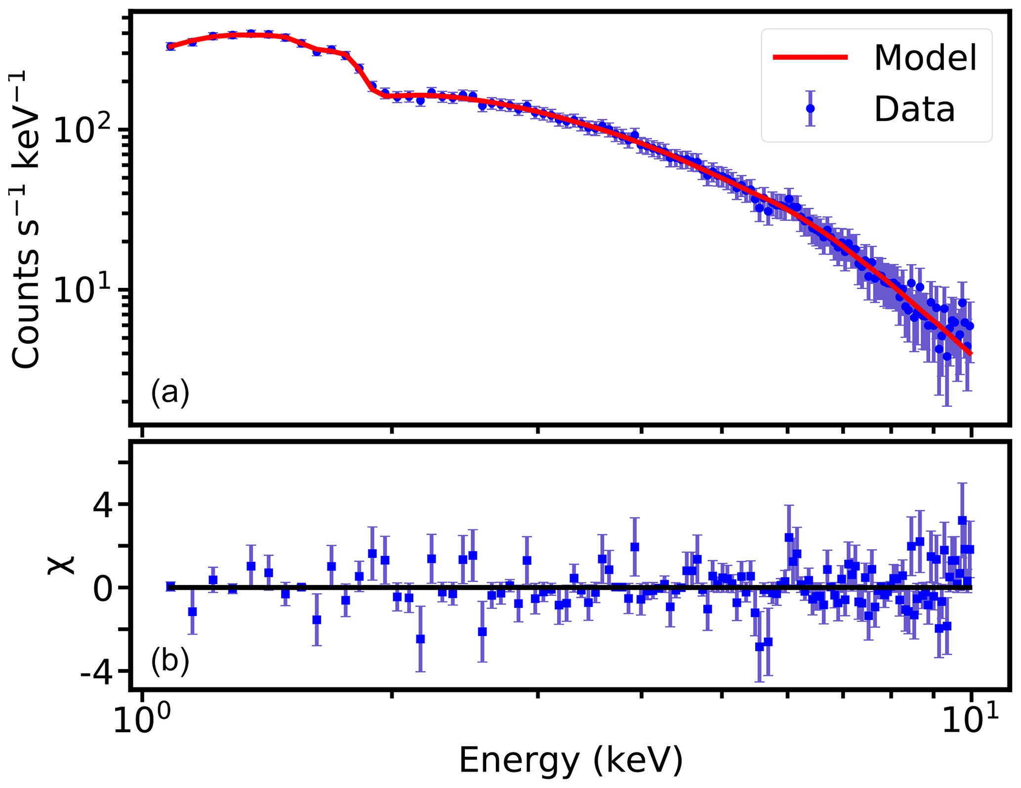
Figure 8(a) The best-fit model and the data of unattenuated spectrum for the Crab Nebula from LE. The blue dots with error bars are observation data, and the solid red line is the best-fit model. (b) The residuals ((data−model) / error) of the fit.
The main atmospheric components causing extinction are oxygen (O, O2), nitrogen (N, N2), and argon during the occultation. The absorption of N and O to X-ray has similar characteristics because the energy dependence of the X-ray cross sections of N and O is similar in our interest energy band (Katsuda et al., 2021). In other words, it is impossible to distinguish N and O through X-ray occultation in our interest energy band, but their total atmospheric density (N + O + O2 + N2) distribution can be calculated. In addition, although X-ray photons interact directly with the K- and L- shell electrons of atoms (including atoms within molecules), the O2 (or N2) counts as one absorbing “particle” in the calculation. Ar is an atmospheric constituent of less content relative to N and O in the Earth's atmosphere. The atmospheric density of Ar is 0.029 %–0.943 % of the total density of N and O according to the NRLMSISE-00 model in the altitude range of 20–200 km. But the X-ray cross section of Ar is larger by almost 1 order of magnitude than that of N and O over the energy range of interest. Therefore, Ar is included in our model.
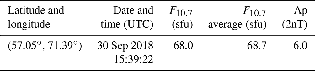
The number density of each atmospheric component needs to be given as input data in the process of density profile retrieval with a forward model (Determan et al., 2007). In the following, the atmospheric models NRLMSISE-00 and NRLMSIS 2.0 (Emmert et al., 2021) are chosen as our input data in the modelling. The NRLMSISE-00 model is one of the most widely used and relatively accurate atmospheric model for the Earth's upper and middle atmosphere. The NRLMSIS 2.0 model is an upgraded version of the NRLMSISE-00 model. The input parameters of NRLMSISE-00 and NRLMSIS 2.0 for the calculation of model atmospheric density are listed in Table 3. In Table 3, the time corresponds to the middle tangent point altitude during occultations. The geographical latitude and longitude are calculated with coordination transformation from the coordination of the tangent point in J2000. F10.7 and Ap are the solar activity index and the geomagnetic activity at this time. The F10.7 index is one of the most widely used indices to characterize the level of solar activity (Tapping, 2013), and the Ap index is used to characterize the geomagnetic activity (Clúa de Gonzalez et al., 1993). These data are obtained from the Space Environment Prediction Center (http://eng.sepc.ac.cn/index.php, last access: 7 May 2022).
The X-ray cross section σs of each component of the gas can be obtained through the photon cross section database XCOM (Berger and Hubbell, 1987; Berger et al., 2010). The X-ray cross sections of Ar, O, and N are shown in Fig. 2.
Table 3The input parameters of NRLMSISE-00 for the calculation of the model atmospheric density profile.
The specific form of the forward model of X-ray occultations is as follows (Determan et al., 2007):
where R is the detector response matrix (Li et al., 2020). In addition, the forward model also contains background noise B. The background noise should be included in the forward model, as shown in Eq. (3).
3.2 Density profile retrieval
Instead of subtracting the background, the background and the source counts can be modelled synchronously using Poisson statistics in the Bayesian framework (Olamaie et al., 2014). Bayes' theorem combines observation data with the prior distribution of the parameter of interest θ from a specific model to obtain the posterior probability distribution of the parameter. In this work, the posterior probability distribution of for the forward model shown in Eq. (3) applied to the data D can be given by Bayes' theorem (Bayes and Price, 1763):
where D is the observation data, M is the forward model, p(θ|M) is the prior distribution, is the likelihood, and p(D|M) is the Bayesian evidence.
Both the X-ray-observed counts and the background data follow Poisson statistics, so that the X-ray likelihood function, ℒ, is given by
where Di is the observation data in the ith bin, and Mi is the ith forward model value. The natural logarithm of the likelihood function can also be used for parameter estimation as the C statistic (Cash, 1979).
In this paper, we analyse the light curve in the energy range of 1.0–2.5, 2.5–6.0, and 6.0–10.0 keV; it is found that these energy ranges are indeed sensitive to the altitude range of 105–200, 95–125, and 85–110 km, respectively, as shown in Fig. 9. The red shading in Fig. 9 indicates the occultation range, and the blue shading in Fig. 9 indicates the energy range.
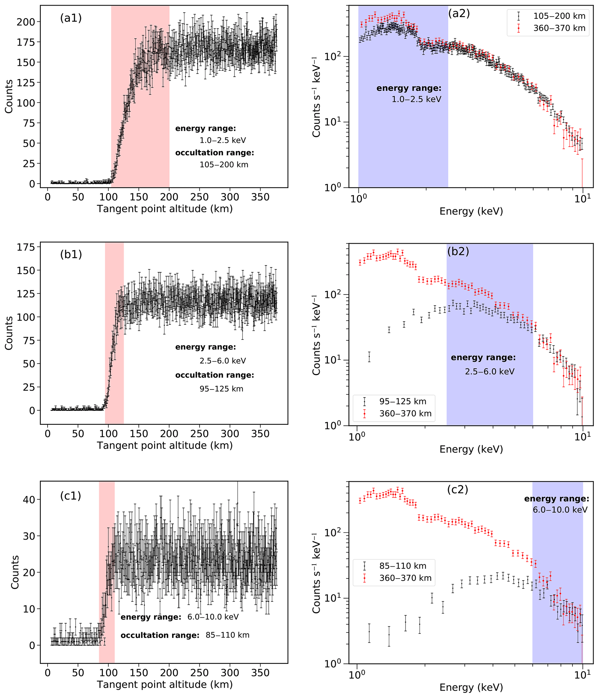
Figure 9Light curve and energy spectrum during occultation. Panel (a1) represents the light curve in the energy range of 1.0–2.5 keV, and it is found that this energy band is indeed sensitive to the altitude range of 105–200 km. Panel (a2) shows the comparison between the energy spectrum in the altitude range of 105–200 km and the unattenuated energy spectrum, and it is found that there is a significant attenuation of the energy spectrum in the altitude range in the range of 1.0–2.5 keV. Panel (b1) represents the light curve in the energy range of 2.5–6.0 keV, and it is found that this energy band is indeed sensitive to the altitude range of 95–125 km. Panel (b2) shows the comparison between the energy spectrum in this altitude range and the unattenuated energy spectrum, and it is found that the energy spectrum in this altitude range has significant attenuation in the energy range of 2.5–6.0 keV. Panel (c1) represents the light curve in the energy range of 6.0–10.0 keV, which is indeed sensitive to the altitude range of 85–110 km. Panel (c2) shows the comparison between the energy spectrum in this altitude range and the unattenuated energy spectrum, and it is found that the energy spectrum in this altitude range has significant attenuation in the energy range of 6.0–10.0 keV. The red shading marks the occultation range, and the blue shading marks the energy range.
The Markov chain–Monte Carlo (MCMC) method is one of the parameter estimation methods used for Bayesian inference (Sharma, 2017).
The density profile retrieval implements the MCMC method, which samples from a probability distribution using Markov chains (Chib and Greenberg, 1995; Dunkley et al., 2005; Hogg and Foreman-Mackey, 2018).
MCMC is implemented by emcee (Foreman-Mackey et al., 2013) that uses an affine-invariant ensemble sampler. A total of 200 000 steps with 10 walkers are used in the sampling process. A 20 000-step MCMC chain for each walker led to 1 standard deviation estimates for the correction factor γs and the background B as [0.871–0.905] and [0.609–0.720], [0.787–0.834] and [0.797–0.924], and [0.811–0.948] and [1.399–1.558] based on NRLMSISE-00 and to 1 standard deviation estimates for the correction factor γs and the background B as [1.075–1.118] and [0.621–0.735], [0.897–0.951] and [0.793–0.919], and [0.936–1.905] and [1.398–1.558] based on NRLMSIS 2.0 in the energy range of 1.0–2.5, 2.5–6.0, and 6.0–10.0 keV, respectively, where the first 1000 steps in each walker are burned.
The posterior probability distribution of the correction factor γs and the background B is obtained, as shown in Fig. 10.
In this corner plot, the vertical dashed black lines are the quantiles 0.16 and 0.84 of the posterior probability distribution respectively. The vertical dashed red line indicates the median for the posterior probability distribution of the correction factor γs and the background B.
The median of the posterior probability distribution and the interval with the quantiles of 0.16 and 0.84 are marked above the histogram. The retrieved results of atmospheric density can be obtained by multiplying γs by the input data. Therefore, γs can be used as an average scaling factor for NRLMSISE-00 and NRLMSIS 2.0 density models.
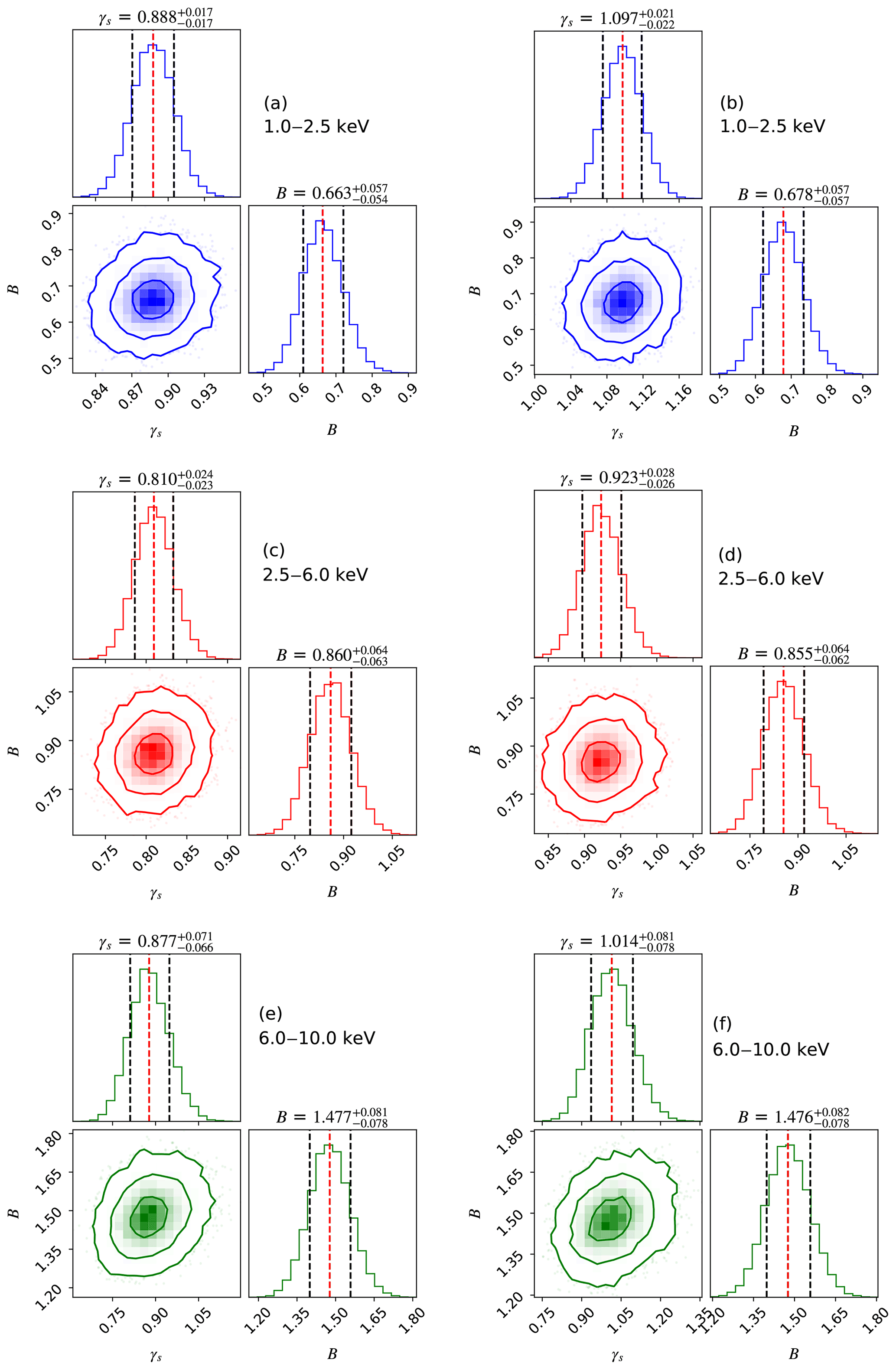
Figure 10Corner plot showing the one- and two-dimensional projections of the posterior probability distributions for the two free parameters. On the 2D plots, blue, red, and green contours represent 1-, 2-, and 3σ confidence intervals. The dashed black lines in each of the 1D histograms represent the quantiles 0.16 and 0.84 of the posterior probability distribution, with the central dashed red line indicating the median value. The median ± the 68 % confidence interval is shown above each histogram. Panels (a) and (b) represent posterior probability distributions based on NRLMSISE-00 and NRLMSIS 2.0, respectively, by fitting the light curves in 1.0–2.5 keV. Panel (c) and (d) represent posterior probability distributions based on NRLMSISE-00 and NRLMSIS 2.0, respectively, by fitting the light curves in 2.5–6.0 keV. Panel (e) and (f) represent posterior probability distributions based on NRLMSISE-00 and NRLMSIS 2.0, respectively, by fitting the light curves in 6.0–10.0 keV.
The comparison for the retrieved density profile with XEOS in the energy range of 1.0–2.5, 2.5–6.0, and 6.0–10.0 keV, the previous retrieval results based on RXTE in the altitude range of 100–120 km (Determan et al., 2007), the NRLMSISE-00 model density profile, and the NRLMSIS 2.0 model density profile are shown in Fig. 11. The density profiles marked by the legend of Insight-HXMT (XEOS-00) and Insight-HXMT (XEOS-2.0) in each panel in Fig. 11 are the retrieved results based on the NRLMSISE-00 model and the NRLMSIS 2.0 model, respectively. There is an obvious gap between the XEO measurement and the model prediction from NRLMSISE-00. The retrieved density profiles from Insight-HXMT based on the NRLMSISE-00 and NRLMSIS 2.0 models by fitting the light curves in the energy range of 1.0–2.5, 2.5–6.0, and 6.0–10.0 keV are qualitatively consistent with the previous retrieved results from RXTE, and there are two intersections between the retrieved density with Insight-HXMT by fitting the light curve in the energy range of 2.5–6.0 keV and the retrieved density from RXTE. The XEO-retrieved density is approximately 88.8 % of the density of the NRLMSISE-00 model and 109.7 % of the density of the NRLMSIS 2.0 model in the altitude range of 105–200 km at the same time and location, respectively. The XEO-retrieved density is approximately 81.0 % of the density of the NRLMSISE-00 model and approximately 92.3 % of the density of the NRLMSIS 2.0 model in the altitude range of 95–125 km at the same time and location, respectively. The XEO-retrieved density is approximately 87.7 % of the density of the NRLMSISE-00 model and 101.4 % of the density of the NRLMSIS 2.0 model in the altitude range of 85–110 km at the same time and location, respectively. The previous retrieval density based on RXTE by XEOS is approximately 50 % of the density of the NRLMSISE-00 model in the altitude range of 100–120 km on 14 November 2005. The latest semi-empirical atmospheric model, NRLMSIS 2.0, which belongs to the MSIS family, has recently been released, and it is a significant upgrade of the previous version, NRLMSISE-00. The density profile from NRLMSIS 2.0 is about 8.5 %–21.9 % lower than the densities from NRLMSISE-00 in the altitude range of 95–125 km. Nevertheless, the gap between the retrieved density profile and the model prediction from NRLMSISE-00 and NRLMSIS 2.0 still needs to be verified further.
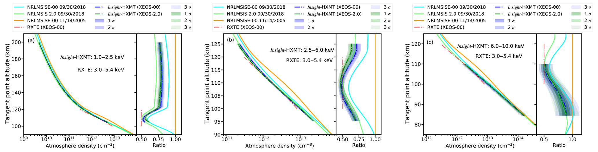
Figure 11Panel (a) shows the comparison between the retrieved density profile in the altitude range of 105–200 km based on the XEOS method and the NRLMSISE-00 and NRLMSIS 2.0 model predictions as well as the previous retrieved results based on PCA/RXTE. Panel (b) shows the comparison between the retrieved density profile in the altitude range of 95–125 km based on the XEOS method and the NRLMSISE-00 and NRLMSIS 2.0 model predictions as well as the previous retrieved results based on PCA/RXTE. Panel (c) shows the comparison between the retrieved density profile in the altitude range of 85–110 km based on the XEOS method and the NRLMSISE-00 and NRLMSIS 2.0 model predictions as well as the previous retrieved results based on PCA/RXTE. Right sub-panel of each panel: all density profiles are normalized to the NRLMSISE-00 density profile on 14 November 2005, in order to visually compare the differences between the various density profiles.
Comparisons between the observed light curve data points and the model light curves based on the best-fit density profiles and model-predicted light curves based on the NRLMSISE-00 and NRLMSIS 2.0 model simulation are shown in Fig. 12. Panels (a), (b), and (c) indicate the light curves in the energy range of 1.0–2.5, 2.5–6.0, and 6.0–10.0 keV, respectively. The residuals between observed light curves and model light curves are also shown in Fig. 12. For clarity, the data points for observed light curve in Fig. 12 are displayed by taking one point every three points from the initial data points, and the residuals corresponding to the four light curves are shifted vertically in the lower sub-panel of each panel. Four extinction curves of each panel are obtained using the forward model based on the four density profiles for comparison with the XEO observation data, among which the density profiles mainly include the two XEOS-retrieved density profiles and the NRLMSISE-00- and NRLMSIS 2.0-model-predicted density profile for approximately the same date, time, and geographic latitude and longitude. In order to show the difference between the light curves, we amplified the observed light curve and the four model light curves in the altitude range of 120–124, 106–109, and 95–100 km in Fig. 12a, b, and c, respectively.
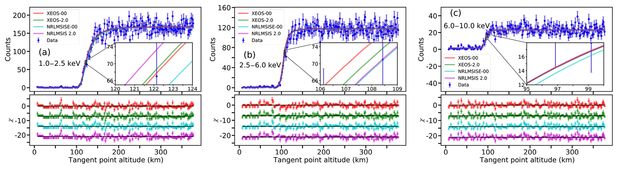
Figure 12Panel (a) represents the comparison between the observed light curve and best-fit light curves from XEOS measurement based on NRLMSISE-00 and NRLMSIS 2.0 as well as the model light curve based on the NRLMSISE-00 and NRLMSIS 2.0 model predictions in the energy range of 1.0–2.5 keV. Panel (b) represents the comparison between the observed light curve and best-fit light curves from XEOS measurement based on NRLMSISE-00 and NRLMSIS 2.0 as well as the model light curve based on the NRLMSISE-00 and NRLMSIS 2.0 model predictions in the energy range of 2.5–6.0 keV. Panel (c) represents the comparison between the observed light curve and best-fit light curves from XEOS measurement based on NRLMSISE-00 and NRLMSIS 2.0 as well as the model light curve based on the NRLMSISE-00 and NRLMSIS 2.0 model predictions in the energy range of 6.0–10.0 keV. Lower sub-panel of each panel: the residuals between the observed light curve and best-fit light curves, model light curves based on NRLMSISE-00 and NRLMSIS 2.0. The colour of residuals corresponds to the colour of the best-fit light curves or model light curves. The residuals corresponding to the four light curves are shifted vertically for clarity.
3.3 Testing results
In this section, Pearson's χ2 test (Pearson, 1900; Cochran, 1952) is used to test the XEO measurements and NRLMSISE-00 and NRLMSIS 2.0 model prediction for the description of the XEO light curve.
In this study, the following null hypotheses are proposed. The light curves predicted by the XEO-measured density profile and the NRLMSISE-00- and NRLMSIS 2.0-model-simulated density profile fit the observed light curve well. It is found that the null hypothesis can not be rejected even at the 84 % and 90 % confidence level for the two XEO measurements in the energy range of 1.0–2.5 keV, the null hypothesis can not be rejected even at the 55 % and 64 % confidence level for the two XEO measurements in the energy range of 2.5–6.0 keV, and the null hypothesis can not be rejected even at the 68 % and 69 % confidence level for the two XEO measurements in the energy range of 6.0–10.0 keV, as shown in Table 4. It is found that the null hypothesis can not be rejected at the 95 % confidence level for both the NRLMSISE-00 and NRLMSIS 2.0 predictions, except for the NRLMSISE-00 predictions by the model light curve in the energy range of 1.0–2.5 keV. Goodness-of-fit testing results between the observed light curve and the extinction curve predictions with XEO-measured density profiles and the NRLMSISE-00- and NRLMSIS 2.0-model-simulated density profiles are also listed in Table 4.
Goodness-of-fit testing is carried out for the observed light curve and four model light curves in the energy range of 1.0–2.5 keV. As shown in Table 4, the and p value between the observed light curve and the extinction curve predicted with the XEO-retrieved density profile based on NRLMSISE-00 are 1.0599 and 0.1604, where dof represents the degrees of freedom, i.e., the number of sample points minus the number of variables. In this paper, 551 sample points are used for fitting, with two variables of correction factor and background noise, so dof = 549. The and p value between the observed light curve and the extinction curve predicted with the XEO-retrieved density profile based on NRLMSIS 2.0 are 1.0756 and 0.1074. The and p value between the observed light curve and the extinction curve predicted with the NRLMSISE-00-predicted density profile are 1.1220 and 0.0249. The and p value between the observed light curve and the extinction curve predicted with the NRLMSIS 2.0-predicted density profile are 1.0783 and 0.0997. The results show that the light curves based on XEO-retrieved density can better describe the observed light curve. Compared with the retrieved results, the atmospheric density predicted by the NRLMSISE-00 model overestimates by 11.2 %, and the atmospheric density predicted by the NRLMSIS 2.0 model underestimates by 9.7 %.
Goodness-of-fit testing is carried out for the observed light curve and four model light curves in the energy range of 2.5–6.0 keV. As shown in Table 4, the and p value between the observed light curve and the extinction curve predicted with the XEO-retrieved density profile based on NRLMSISE-00 are 1.0091 and 0.4540. The and p value between the observed light curve and the extinction curve predicted with the XEO-retrieved density profile based on NRLMSIS 2.0 are 1.0612 and 0.3669. The and p value between the observed light curve and the extinction curve predicted with the NRLMSISE-00-predicted density profile are 1.3321 and 0.0802. The and p value between the observed light curve and the extinction curve predicted with the NRLMSIS 2.0-predicted density profile are 1.3331 and 0.0797. It is found that the light curve predictions based on the XEO-retrieved density profiles can describe the observed light curve better, and gaps between the retrieved density profiles and the model-simulated ones exist. Compared with our retrieved results, the density profile of the NRLMSISE-00 model is overestimated by 19 %, and the density profile of the NRLMSIS 2.0 model is overestimated by 7.7 %.
Goodness-of-fit testing is carried out for the observed light curve and four model light curves in the energy range of 6.0–10.0 keV. As shown in Table 4, the and p value between the observed light curve and the extinction curve predicted with the XEO-retrieved density profile based on NRLMSISE-00 are 1.0936 and 0.3293. The and p value between the observed light curve and the extinction curve predicted with the XEO-retrieved density profile based on NRLMSIS 2.0 are 1.1012 and 0.3193. The and p value between the observed light curve and the extinction curve predicted with the NRLMSISE-00-predicted density profile are 1.2085 and 0.1967. The and p value between the observed light curve and the extinction curve predicted with the NRLMSIS 2.0-predicted density profile are 1.0955 and 0.3268. The results show that the light curves based on XEO-retrieved density and the NRLMSIS 2.0-predicted density can better describe the observed light curve. The retrieved results based on the light curve in the energy range of 6.0–10.0 keV are basically consistent with the model density of NRLMSIS 2.0, but the density profile of NRLMSISE-00 is overestimated by about 12.3 %.
From the above results, it is found that the altitude ranges that correspond to the light curve attenuations are indeed sensitive to different energy ranges, and they often overlap. For example, the energy band of 1.0–2.5 keV is sensitive to the altitude range of 105–200 km, and the energy band of 6.0–10.0 keV is sensitive to the altitude range of 85–110 km. Therefore, the overlap range between the sensitive altitude ranges for the two energy bands is 105–110 km. But the retrieved density profiles of different energy bands are different in the overlap altitude range. This is because the XEOS retrieval by light curve fitting is an altitude-dependent method, different energy bands have different sensitive altitude ranges, and the retrieved results can be different, even if there are overlapping altitude areas. The retrieved results are a simple scaling of MSIS density. The occultation data of X-ray detectors with larger effective area or stronger detection ability can be used to retrieve atmospheric density to reduce the influence of energy integration.
Table 4Hypothesis testing results for the extinction curve predictions with XEO-measured density profiles and NRLMSISE-00- and NRLMSIS 2.0-model-simulated density profiles (during the occultation).


Figure 13Comparison of the observed data and forward model light curves under extreme solar activity, very low solar activity, severe geomagnetic storm, and quiet geomagnetic activity. The NRLMSISE-00 density profiles are used as input data for those simulations. For clarity, the data points are displayed by taking one point every five points from the initial data points. The energy range of the light curves in panel (a), (b), and (c) is 1–2.5, 2.5–6.0, and 6.0–10.0 keV, respectively. Furthermore, local magnification of the light curves in the altitude range of 105–150, 95–125, and 85–110 km is carried out to show the influence of solar and geomagnetic activities on the shape of the model light curves in panel (a), (b), and (c), respectively.
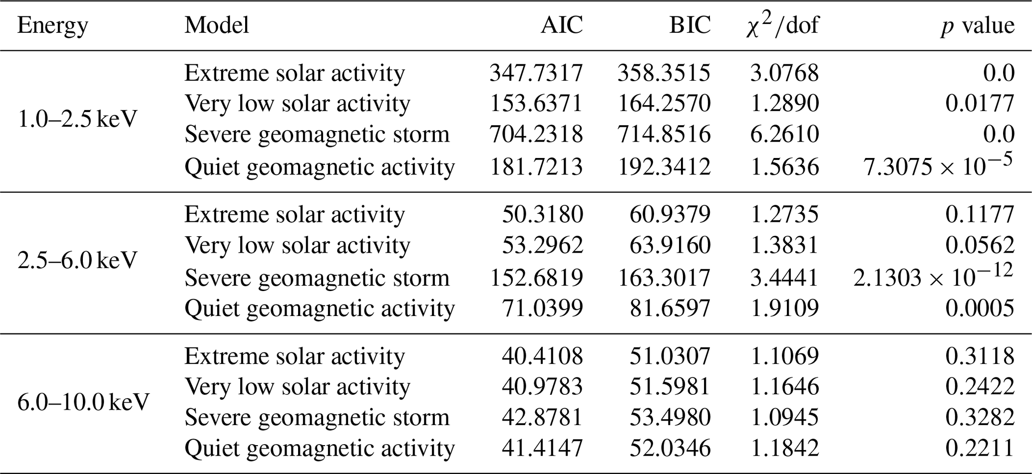
Since the Earth's middle and upper atmosphere is greatly affected by solar activity and geomagnetic activity, it will also have an impact on the density of the Earth's upper and middle atmosphere, so the possible systematic uncertainty of the predicted XEO light curve due to variations of solar and geomagnetic activity is discussed. Common solar activity includes sunspots, flares, and corona. Here, the effects can be demonstrated by the predicted XEO light curve with the NRLMSISE-00 density profile for the changing solar activity index F10.7 and geomagnetic activity index Ap. The values of the model light curves under extreme solar activity, very low solar activity (Licata et al., 2020), a severe geomagnetic storm, and quiet geomagnetic activity (Palacios et al., 2018) are calculated, as shown in Fig. 13. The energy range of the light curve in Fig. 13a–c is 1.0–2.5, 2.5–6.0, and 6.0–10.0 keV, respectively. For clarity, the data points are displayed by taking one point every five points from the initial data points in Fig. 13. In order to show the difference between the light curves under the different solar activities and geomagnetic activities, the observed light curve and the model light curves in the altitude range of 105–150, 95–125, and 85–110 km are locally amplified in Fig. 13a, b, and c, respectively. The Akaike information criterion (AIC) and the Bayesian information criterion (BIC) are calculated for these model comparisons, and the results are listed in Table 5. AIC and BIC are used for model selection and can also be used to compare models. Usually, we choose the model with the smallest AIC and BIC. However, the values of AIC and BIC in this paper show that solar and geomagnetic activity has a great influence on model shape. because AIC and BIC values vary greatly under different solar and geomagnetic activity in a relatively low energy range. Goodness of fit between the observed light curve and the model light curves under the different solar activities and geomagnetic activities is also evaluated by the and p value in Table 5. It can be shown that the solar activity and the geomagnetic activity have great influence on the shape of model light curves. In addition, with the increase of altitude, solar and geomagnetic activities have a greater impact on the model light curves. The effects of solar activities and geomagnetic storms on the XEO light curve modelling and density retrieval will be further investigated in the future.
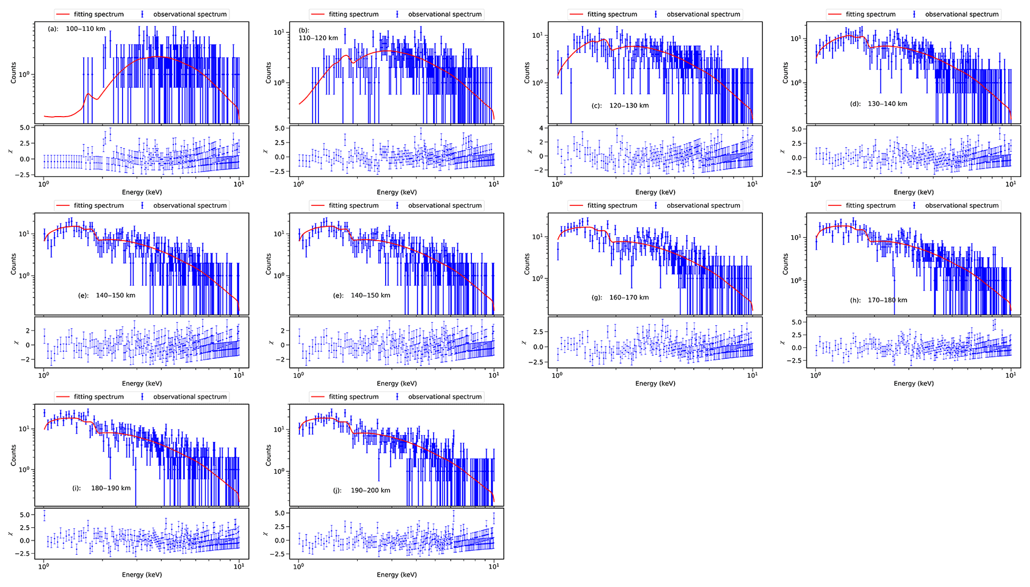
Figure 14Comparison of best-fit spectrum model and observational spectrum data. In the upper space of each panel, blue dots with error bars represent data points, solid red lines represent best-fit spectrum models, and the lower space of each panel represents residuals between the best-fit model and observational spectrum data.
3.4 Comparison to the results from an altitude-independent method by spectrum fitting
Based on the energy spectrum fitting method during X-ray occultation (Katsuda et al., 2021; Yu et al., 2022), the altitude-independent atmospheric-density-retrieved results can be obtained, and the overlap of the tangent point altitude can be effectively avoided. In order to prove the reliability of our retrieved results in the paper, we compare our results with the results of energy spectrum fitting (Yu et al., 2022). The optical depth of the forward model based on energy spectrum fitting is given by the following equation:
where γh represents correction factors in different altitudes ranges. By combining Eqs. (3) and (6), the forward model of the energy spectrum fitting for different altitude ranges is given. By fitting the energy spectrum data in different altitude ranges, the correction factors in corresponding altitude ranges can be obtained, namely γh. So multiplying γh with the input data from the NRLMSIS 2.0 model, the atmospheric density in different altitude ranges can be retrieved independently.
In the paper, by fitting the energy spectrum data in the energy range of 1–10 keV, we obtain the atmospheric density values in the altitude range of 100–200 km and extract the energy spectrum data every 10 km. The comparison between the best-fit model and energy spectrum observational data is shown in Fig. 14. The retrieved results based on energy spectrum fitting and the results with light curve fitting are shown in Fig. 15, where the solid blue line represents the retrieved results of spectrum fitting, the solid red line represents the model density profile of NRLMSIS 2.0, and the solid green line represents the retrieved results with light curve fitting in the energy range of 1.0–2.5 keV. It is found that the retrieved results based on the light curve fitting are qualitatively consistent with the retrieved results of the energy spectrum fitting method. In the altitude range of 180–200 km, because the number of X-ray photons absorbed by the Earth's atmosphere is less than the X-ray photon counting error, the retrieved results based on energy spectrum fitting have large uncertainty. However, the reliability of the results based on light curve fitting is proved to be consistent with that by the altitude-independent method by spectrum fitting.
In this paper, we have studied the X-ray Earth occultation of the Crab Nebula with the pointing observation data from Insight-HXMT. We have presented a detailed Bayesian data analysis method for the extinction light curve modelling from the X-ray Earth occultation process. The theoretical predicted XEO observational light curve is calculated with the light curve forward model. The data recorded by the low-energy X-ray telescope (LE) of Insight-HXMT are analysed, and the density profile is retrieved. The results are tested and validated with the measurements from the RXTE satellite and the retrieval results with the altitude-independent method by spectrum fitting.
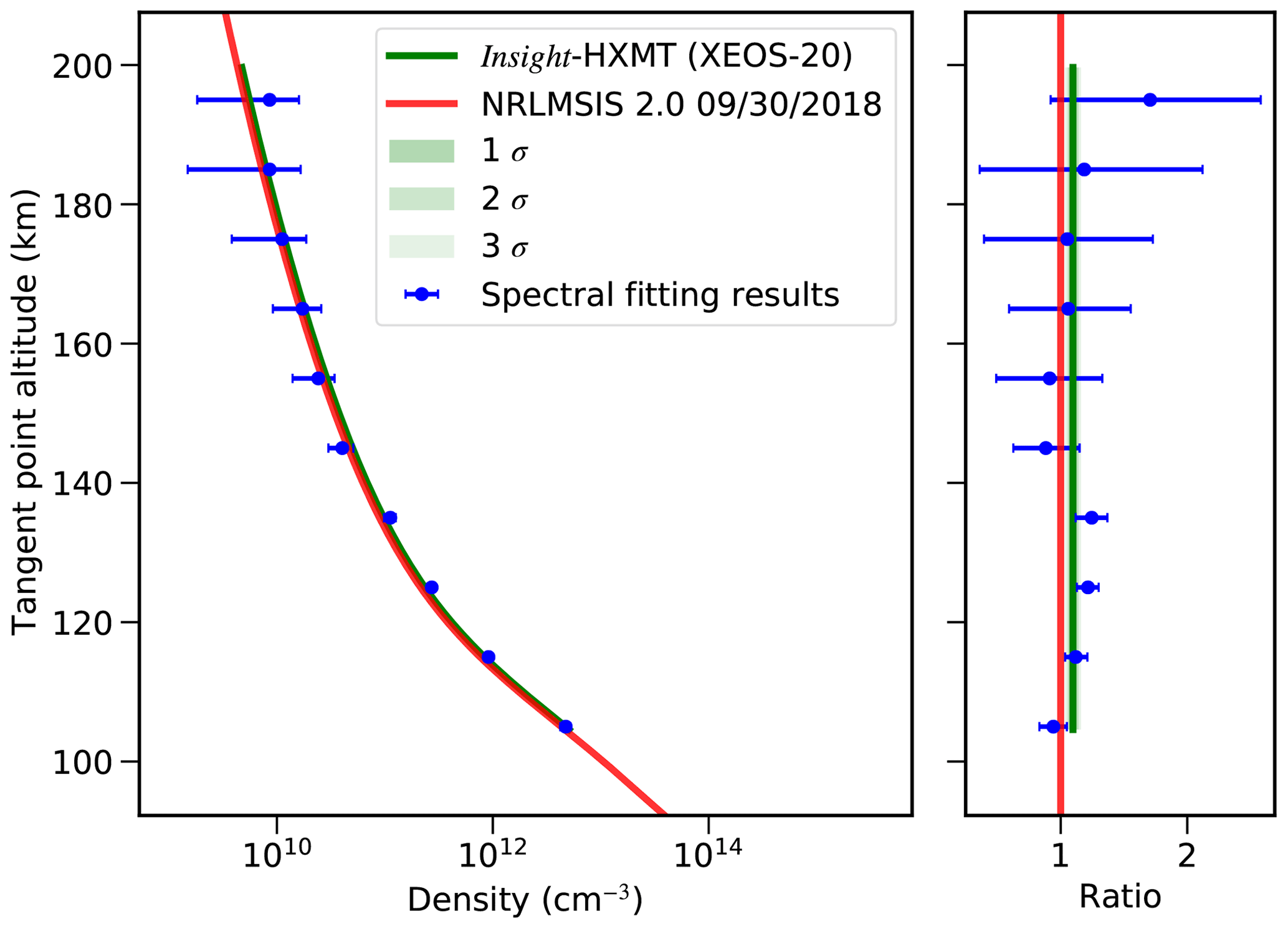
Figure 15Comparison of retrieved results based on energy spectrum fitting and light curve fitting. The solid blue line represents the retrieved results of spectrum fitting, the solid red line represents the model density profile of NRLMSIS 2.0, and the solid green line represents the retrieved results of the light curve in the energy range of 1.0–2.5 keV. Right panel: all density profiles are normalized to the NRLMSISE 2.0 density profile on 30 September 2018.
We have shown from the XEO extinction light curve modelling that the X-ray astronomical satellite Insight-HXMT can be used to retrieve atmospheric density by the X-ray Earth occultation of celestial sources. The XEO-retrieved density profile in the altitude range of 105–200 km by fitting the light curves in the energy range of 1.0–2.5 keV is lower than the density of NRLMSISE-00 and larger than the density of NRLMSIS 2.0 for the same date, time, and geographical location. The results show that the retrieved density profiles are 88.8 % of the NRLMSISE-00 density and 109.7 % of the NRLMSIS 2.0 density in the altitude range of 105–200 km. The XEO-retrieved density profile in the altitude range of 95–125 km by fitting the light curves in the energy range of 2.5–6.0 keV is lower than the NRLMSISE-00- and NRLMSIS 2.0-model-predicted density profile for the same date, time, and geographical location. It is found that the retrieved density profile is 81.0 % of the density prediction by NRLMSISE-00, and the retrieved density profile is 92.3 % of the density prediction by NRLMSISE 2.0 in an altitude range of 95–125 km, respectively. The XEO-retrieved density profile in the altitude range of 85–110 km by fitting the light curves in the energy range of 6.0–10.0 keV is lower than the NRLMSISE-00 density but almost consistent with the density of the NRLMSIS 2.0 model. Moreover, the XEO-retrieved density profiles and the NRLMSIS 2.0 density can better describe the light curve than the density of NRLMSISE-00 for the same time, date, and location. The results show that the XEO-retrieved density profiles are 87.7 % of the NRLMSISE-00 density and 101.4 % of the NRLMSIS 2.0 density. The retrieved density profiles with LE/Insight-HXMT are qualitatively consistent with the retrieved density with RXTE, especially in the altitude range of 95–125 km, and there are two intersections between the XEO-retrieved density and the measurement of RXTE. This shows that the Insight-HXMT, as an atmospheric diagnostic instrument, further validates the difference between the measurements from the X-ray satellite and the model density. The Insight-HXMT satellite with other X-ray astronomical satellites in orbit can form a space observation network for XEOS in the future (https://heasarc.gsfc.nasa.gov/, last access: 7 May 2022). In addition, it is found that the sensitive altitude ranges of different energy bands often overlap, and the retrieved atmospheric densities of the overlapping regions obtained by fitting the light curves of different energy ranges are often different. The light curve fitting method is an altitude-dependent method. Different energy bands have different sensitive altitude ranges, and the retrieved results are different, even if there is an overlapping altitude range. In other words, an averaged scale factor for density profile in an altitude range is obtained by the light curve fitting method. We confirmed the measured density profile from light curve fitting through comparison to the ones by a standard spectrum retrieval method with an iterative inversion technique. The occultation data from larger effective areas can be used to retrieve atmospheric density to reduce the influence of energy integration. A more detailed description of this problem will be discussed in the future.
The difference between the measured and model values may result from the long-term accumulation of greenhouse gases, imperfect climatological estimates of solar and geomagnetic effects, differences in temperature profiles, and the influence of gravity waves (Determan et al., 2007; Katsuda et al., 2021). And the differences can also be due to model errors and/or retrieval errors. In order to further clarify and explain the difference, a large number of X-ray occultation data from past, present, and future X-ray satellites will be required for further analysis. However, the atmospheric density retrieval method in this study depends on atmospheric models. The retrieved results vary with the shape of density profiles for different atmospheric models. Therefore, model-independent retrieval methods needs to be developed, and we will consider this kind of XEOS method in the future.
X-ray photons with higher energy can penetrate deeper into the Earth's atmosphere. The observation data of HE and ME (Liu et al., 2020; Cao et al., 2020) will be analysed in our future work. In addition, we will investigate the factors for affecting the XEO light curve modelling and density retrieval, such as the extended X-ray source effects and the energy spectra variations. These effects for the XEO light curve modelling and density retrieval will be analysed in the next work.
Datasets related to the paper are available from http://archive.hxmt.cn/proposal (HXMT, 2022; last access: 7 May 2022).
BL and HL were responsible for conceptualization. HL was responsible for funding acquisition and supervision. HL was responsible for the forward model building, the retrieval algorithm, and the original software development. DY and YT were responsible for the data reduction. DY, HL, and YL were involved in the software update and data analysis. HL and MG were responsible for the design of the observations. XL and WX were responsible for the validation of the results. DY prepared the original draft. All co-authors reviewed and edited the paper.
The contact author has declared that neither they nor their co-authors have any competing interests.
Publisher's note: Copernicus Publications remains neutral with regard to jurisdictional claims in published maps and institutional affiliations.
Haitao Li thanks Viktoria Sofieva (Finnish Meteorological Institute) and Xiaocheng Wu (National Space Science Center, CAS) for discussion and help with the treatment of the Abel integral. This work was supported by the Youth Innovation Promotion Association CAS (grant no. 2018178), the National Natural Science Foundation of China (grant nos. 41604152, U1938111, U1938109, U1838104, and U1838105), and the National Key Research and Development Program of China (grant nos. 2017YFB0503300 and 2016YFA0400800). This work made use of the data from the HXMT mission, a project funded by the China National Space Administration (CNSA) and the Chinese Academy of Sciences (CAS). We greatly appreciate the anonymous referees for the insightful comments that helped improve the quality of this work.
This research has been supported by the Youth Innovation Promotion Association of the Chinese Academy of Sciences (grant no. 2018178), the National Natural Science Foundation of China (grant nos. 41604152, U1938111, U1938109, U1838104, and U1838105), and the National Key Research and Development Program of China (grant nos. 2017YFB0503300 and 2016YFA0400800).
This paper was edited by Alyn Lambert and reviewed by two anonymous referees.
Aikin, A. C., Hedin, A. E., Kendig, D. J., and Drake, S.: Thermospheric molecular oxygen measurements using the ultraviolet spectrometer on the Solar Maximum Mission spacecraft, J. Geophys. Res.-Space Phys., 98, 17607–17614, https://doi.org/10.1029/93JA01468, 1993. a
Arnaud, K., Dorman, B., and Gordon, C.: XSPEC: An X-ray spectral fitting package, Astrophysics Source Code Library, record ascl:9910.005, 1999. a
Baron, P., Ochiai, S., Dupuy, E., Larsson, R., Liu, H., Manago, N., Murtagh, D., Oyama, S., Sagawa, H., Saito, A., Sakazaki, T., Shiotani, M., and Suzuki, M.: Potential for the measurement of mesosphere and lower thermosphere (MLT) wind, temperature, density and geomagnetic field with Superconducting Submillimeter-Wave Limb-Emission Sounder 2 (SMILES-2), Atmos. Meas. Tech., 13, 219–237, https://doi.org/10.5194/amt-13-219-2020, 2020. a
Bartman, F. L., Chaney, L. W., Jones, L. M., and Liu, V. C.: Upper-Air Density and Temperature by the Falling-Sphere Method, J. Appl. Phys., 27, 706–712, https://doi.org/10.1063/1.1722470, 1956. a
Bayes, T. and Price, R.: An Essay towards Solving a Problem in the Doctrine of Chances, By the Late Rev. Mr. Bayes, F. R. S. Communicated by Mr. Price, in a Letter to John Canton, A. M. F. R. S., Phil. Trans., 53, 370–418, 1763. a
Berger, C., Biancale, R., Barlier, F., and Ill, M.: Improvement of the empirical thermospheric model DTM: DTM94 – a comparative review of various temporal variations and prospects in space geodesy applications, J. Geod., 72, 161–178, https://doi.org/10.1007/s001900050158, 1998. a
Berger, M. J. and Hubbell, J. H.: XCOM: Photon cross sections on a personal computer, National Bureau of Standards, Washington, DC (USA). Center for Radiation Research, https://doi.org/10.2172/6016002, 1987. a
Berger, M. J., Hubbell, J., Seltzer, S., Chang, S. M., Coursey, J., Sukumar, J. S., Zucker, D., and Olsen, K.: XCOM: Photon Cross Section Database (version 1.5), https://doi.org/10.18434/T48G6X, 2010. a
Bruinsma, S., Thuillier, G., and Barlier, F.: The DTM-2000 empirical thermosphere model with new data assimilation and constraints at lower boundary: accuracy and properties, J. Atmos. Sol. Terr. Phys., 65, 1053–1070, https://doi.org/10.1016/S1364-6826(03)00137-8, 2003. a
Cao, X., Jiang, W., Meng, B., Zhang, W., Luo, T., Yang, S., Zhang, C., Gu, Y., Sun, L., Liu, X., Yang, J., Li, X., Tan, Y., Liu, S., Du, Y., Lu, F., Xu, Y., Guan, J., Zhang, S., Wang, H., Li, T., Zhang, C., Wen, X., Qu, J., Song, L., Li, X., Ge, M., Zhou, Y., Xiong, S., Zhang, S., Zhang, Y., Cheng, Z., Zhang, F., Li, M., Liang, X., Gao, M., Yang, E., Liu, X., Liu, H., Yang, Y., and Zhang, F.: The Medium Energy X-ray telescope (ME) onboard the Insight-HXMT astronomy satellite, Sci. China-Phys. Mech. Astron., 63, 249504, https://doi.org/10.1007/s11433-019-1506-1, 2020. a
Cash, W.: Parameter estimation in astronomy through application of the likelihood ratio., Astrophys. J., 228, 939–947, https://doi.org/10.1086/156922, 1979. a
Chen, Y., Cui, W., Li, W., Wang, J., Xu, Y., Lu, F., Wang, Y., Chen, T., Han, D., Hu, W., Zhang, Y., Huo, J., Yang, Y., Li, M., Lu, B., Zhang, Z., Li, T., Zhang, S., Xiong, S., Zhang, S., Xue, R., Zhao, X., Zhu, Y., Zhu, Y., Liu, H., Yang, Y., and Zhang, F.: The Low Energy X-ray telescope (LE) onboard the Insight-HXMT astronomy satellite, Sci. China-Phys. Mech. Astron., 63, 249505, https://doi.org/10.1007/s11433-019-1469-5, 2020. a, b, c
Chib, S. and Greenberg, E.: Understanding the Metropolis-Hastings Algorithm, Am. Stat., 49, 327–335, https://doi.org/10.1080/00031305.1995.10476177, 1995. a
Chou, M. Y., Lin, C. C. H., Tsai, H. F., and Lin, C. Y.: Ionospheric electron density inversion for Global Navigation Satellite Systems radio occultation using aided Abel inversions, J. Geophys. Res., 122, 1386–1399, 2017. a
Clúa de Gonzalez, A. L., Gonzalez, W. D., Dutra, S. L. G., and Tsurutani, B. T.: Periodic variation in the geomagnetic activity: A study based on the Ap index, J. Geophys. Res.-Space Phys., 98, 9215–9232, https://doi.org/10.1029/92JA02200, 1993. a
Cochran, W. G.: The χ2 Test of Goodness of Fit, Ann. Math. Stat., 23, 315–345, 1952. a
Davis, M. C. and White, J. T.: X-43A Flight-Test-Determined Aerodynamic Force and Moment Characteristics at Mach 7.0, J. Spacecr. Rockets, 45, 472–484, https://doi.org/10.2514/1.30413, 2008. a
Degenstein, D. A., Bourassa, A. E., Roth, C., Zawada, D., and Rieger, L. A.: Comparing coincident SAGE III ISS measurements of stratospheric trace species with those measured by OSIRIS, in: AGU Fall Meeting Abstracts, vol. 2018, pp. A41I–3065, 2018. a
Determan, J. R., Budzien, S. A., Kowalski, M. P., Lovellette, M. N., Ray, P. S., Wolff, M. T., Wood, K. S., Titarchuk, L., and Bandyopadhyay, R.: Measuring atmospheric density with X-ray occultation sounding, J. Geophys. Res.-Space Phys., 112, A06323, https://doi.org/10.1029/2006JA012014, 2007. a, b, c, d, e, f
Doornbos, E. and Klinkrad, H.: Modelling of space weather effects on satellite drag, Adv. Space Res., 37, 1229–1239, https://doi.org/10.1016/j.asr.2005.04.097, 2006. a
Doornbos, E., Klinkrad, H., and Visser, P.: Use of two-line element data for thermosphere neutral density model calibration, Adv. Space Res., 41, 1115–1122, https://doi.org/10.1016/j.asr.2006.12.025, 2008. a
Dunkley, J., Bucher, M., Ferreira, P. G., Moodley, K., and Skordis, C.: Fast and reliable Markov chain Monte Carlo technique for cosmological parameter estimation, Mon. Not. R. Astron. Soc., 356, 925–936, https://doi.org/10.1111/j.1365-2966.2004.08464.x, 2005. a
Emmert, J. T., Drob, D. P., Picone, J. M., Siskind, D. E., Jones, M., Mlynczak, M. G., Bernath, P. F., Chu, X., Doornbos, E., Funke, B., Goncharenko, L. P., Hervig, M. E., Schwartz, M. J., Sheese, P. E., Vargas, F., Williams, B. P., and Yuan, T.: NRLMSIS 2.0: A Whole Atmosphere Empirical Model of Temperature and Neutral Species Densities, Earth Space Sci., 8, e01321, https://doi.org/10.1029/2020EA001321, 2021. a
Faire, A. C. and Champion, K. S. W.: Falling sphere measurements of atmospheric density temperature and pressure up to 115 km, in: Space Research Conference, p. 1039, 1965. a
Faucher, G. A., Morrissey, J. F., and Stark, C. N.: Falling sphere density measurements, J. Geophys. Res., 72, 299–305, https://doi.org/10.1029/JZ072i001p00299, 1967. a
Foreman-Mackey, D., Hogg, D. W., Lang, D., and Goodman, J.: emcee: The MCMC Hammer, Pub. Astro. Soc. Pacific, 125, 306, https://doi.org/10.1086/670067, 2013. a
Godet, O., Beardmore, A. P., Abbey, A. F., Osborne, J. P., Cusumano, G., Pagani, C., Capalbi, M., Perri, M., Page, K. L., Burrows, D. N., Campana, S., Hill, J. E., Kennea, J. A., and Moretti, A.: Modelling the spectral response of the Swift-XRT CCD camera: experience learnt from in-flight calibration, Astron. Astrophys., 494, 775–797, https://doi.org/10.1051/0004-6361:200811157, 2009. a
Hajj, G. A. and Romans, L. J.: Ionospheric electron density profiles obtained with the Global Positioning System: Results from the GPS/MET experiment, Radio Sci., 33, 175–190, 1998. a
Haycock, O. C., Westlund, C. D., Pound, E. F., and Woolley, R. H.: Falling Sphere for Measuring Atmospheric Density, Rev. Sci. Instrum., 39, 1094–1099, https://doi.org/10.1063/1.1683591, 1968. a
Hays, P. and Roble, R.: Observation of mesospheric ozone at low latitudes, Planet Space Sci., 21, 273–279, https://doi.org/10.1016/0032-0633(73)90011-1, 1973. a
Hedin, A. E.: MSIS-86 thermospheric model, J. Geophys. Res.-Space Phys., 92, 4649–4662, https://doi.org/10.1029/JA092iA05p04649, 1987. a
Hogg, D. W. and Foreman-Mackey, D.: Data Analysis Recipes: Using Markov Chain Monte Carlo, Astrophys. J. Suppl. Ser., 236, 11, https://doi.org/10.3847/1538-4365/aab76e, 2018. a
Holland, A. and Pool, P.: A new family of swept charge devices (SCDs) for x-ray spectroscopy applications, in: High Energy, Optical, and Infrared Detectors for Astronomy III, edited by Dorn, D. A. and Holland, A. D., vol. 7021 of Society of Photo-Optical Instrumentation Engineers (SPIE) Conference Series, p. 702117, https://doi.org/10.1117/12.797077, 2008. a
HXMT: Proposal, HXMT [data set], http://archive.hxmt.cn/proposal, last access: 7 May 2022. a
Jacchia, L. G.: New Static Models of the Thermosphere and Exosphere with Empirical Temperature Profiles, SAO Special Report, 313, 1970. a
Jacchia, L. G.: Thermospheric Temperature, Density, and Composition: New Models, SAO Special Report, 375, 1977. a
Kalafatoglu Eyiguler, E. C., Shim, J. S., Kuznetsova, M. M., Kaymaz, Z., Bowman, B. R., Codrescu, M. V., Solomon, S. C., Fuller-Rowell, T. J., Ridley, A. J., Mehta, P. M., and Sutton, E. K.: Quantifying the Storm Time Thermospheric Neutral Density Variations Using Model and Observations, Space Weather, 17, 269–284, https://doi.org/10.1029/2018SW002033, 2019. a
Katsuda, S., Fujiwara, H., Ishisaki, Y., Yoshitomo, M., Mori, K., Motizuki, Y., Sato, K., Tashiro, M. S., and Terada, Y.: New Measurement of the Vertical Atmospheric Density Profile From Occultations of the Crab Nebula With X Ray Astronomy Satellites Suzaku and Hitomi, J. Geophys. Res.-Space Phys., 126, e28886, https://doi.org/10.1029/2020JA028886, 2021. a, b, c, d, e, f
Kirsch, M. G., Briel, U. G., Burrows, D., Campana, S., Cusumano, G., Ebisawa, K., Freyberg, M. J., Guainazzi, M., Haberl, F., Jahoda, K., Kaastra, J., Kretschmar, P., Larsson, S., Lubiński, P., Mori, K., Plucinsky, P., Pollock, A. M., Rothschild, R., Sembay, S., Wilms, J., and Yamamoto, M.: Crab: the standard x-ray candle with all (modern) x-ray satellites, in: UV, X-Ray, and Gamma-Ray Space Instrumentation for Astronomy XIV, edited by: Siegmund, O. H. W., vol. 5898 of Society of Photo-Optical Instrumentation Engineers (SPIE) Conference Series, 22–33, https://doi.org/10.1117/12.616893, 2005. a
Krueger, A.: The mean ozone distribution from several series of rocket soundings to 52 km at latitudes from 58∘ S to 64∘ N, Pure Appl. Geophys., 106–108, 1272–1280, 1973. a
Kyrölä, E., Tamminen, J., Sofieva, V., Bertaux, J. L., Hauchecorne, A., Dalaudier, F., Fussen, D., Vanhellemont, F., Fanton d'Andon, O., Barrot, G., Guirlet, M., Fehr, T., and Saavedra de Miguel, L.: GOMOS O3, NO2, and NO3 observations in 2002–2008, Atmos. Chem. Phys., 10, 7723–7738, https://doi.org/10.5194/acp-10-7723-2010, 2010. a
Lei, J., Syndergaard, S., Burns, A. G., Solomon, S. C., Wang, W., Zeng, Z., Roble, R. G., Wu, Q., Kuo, Y. H., Holt, J. M., Zhang, S. R., Hysell, D. L., Rodrigues, F. S., and Lin, C. H.: Comparison of COSMIC ionospheric measurements with ground-based observations and model predictions : Preliminary results, J. Geophys. Res., 112, A07308, https://doi.org/10.1029/2006JA012240, 2007. a
Li, T., Xiong, S., Zhang, S., Lu, F., Song, L., Cao, X., Chang, Z., Chen, G., Chen, L., Chen, T., Chen, Y., Chen, Y., Chen, Y., Cui, W., Cui, W., Deng, J., Dong, Y., Du, Y., Fu, M., Gao, G., Gao, H., Gao, M., Ge, M., Gu, Y., Guan, J., Guo, C., Han, D., Hu, W., Huang, Y., Huo, J., Jia, S., Jiang, L., Jiang, W., Jin, J., Jin, Y., Li, B., Li, C., Li, G., Li, M., Li, W., Li, X., Li, X., Li, X., Li, Y., Li, Z., Li, Z., Liang, X., Liao, J., Liu, C., Liu, G., Liu, H., Liu, S., Liu, X., Liu, Y., Liu, Y., Lu, B., Lu, X., Luo, T., Ma, X., Meng, B., Nang, Y., Nie, J., Ou, G., Qu, J., Sai, N., Sun, L., Tan, Y., Tao, L., Tao, W., Tuo, Y., Wang, G., Wang, H., Wang, J., Wang, W., Wang, Y., Wen, X., Wu, B., Wu, M., Xiao, G., Xu, H., Xu, Y., Yan, L., Yang, J., Yang, S., Yang, Y., Zhang, A., Zhang, C., Zhang, C., Zhang, F., Zhang, H., Zhang, J., Zhang, Q., Zhang, S., Zhang, T., Zhang, W., Zhang, W., Zhang, W., Zhang, Y., Zhang, Y., Zhang, Y., Zhang, Y., Zhang, Z., Zhang, Z., Zhao, H., Zhao, J., Zhao, X., Zheng, S., Zhu, Y., Zhu, Y., and Zou, C.: Insight-HXMT observations of the first binary neutron star merger GW170817, Sci. China-Phys. Mech. Astron., 61, 31011, https://doi.org/10.1007/s11433-017-9107-5, 2018. a
Li, X., Li, X., Tan, Y., Yang, Y., Ge, M., Zhang, J., Tuo, Y., Wu, B., Liao, J., Zhang, Y., Song, L., Zhang, S., Qu, J., nan Zhang, S., Lu, F., Xu, Y., Liu, C., Cao, X., Chen, Y., Nie, J., Zhao, H., and Li, C.: In-flight calibration of the Insight-Hard X-ray Modulation Telescope, J. High Energy Astrophys., 27, 64–76, https://doi.org/10.1016/j.jheap.2020.02.009, 2020. a
Licata, R. J., Tobiska, W. K., and Mehta, P. M.: Benchmarking Forecasting Models for Space Weather Drivers, Space Weather, 18, e02496, https://doi.org/10.1029/2020SW002496, 2020. a
Liu, C., Zhang, Y., Li, X., Lu, X., Chang, Z., Li, Z., Zhang, A., Jin, Y., Yu, H., Zhang, Z., Fu, M., Chen, Y., Ji, J., Xu, Y., Deng, J., Shang, R., Liu, G., Lu, F., Zhang, S., Dong, Y., Li, T., Wu, M., Li, Y., Wang, H., Wu, B., Zhang, Y., Zhang, Z., Xiong, S., Liu, Y., Zhang, S., Liu, H., Yang, Y., and Zhang, F.: The High Energy X-ray telescope (HE) onboard the Insight-HXMT astronomy satellite, Sci. China-Phys. Mech. Astron., 63, 249503, https://doi.org/10.1007/s11433-019-1486-x, 2020. a
Lumpe, J., Fromm, M., Hoppel, K., Bevilacqua, R., Randall, C., Browell, E., Grant, W., McGee, T., Burris, J., Twigg, L., Richard, E., Toon, G., Margitan, J., Şen, B., Pfeilsticker, K., Boesch, H., Fitzenberger, R., Goutail, F., and Pommereau, J.-P.: Comparison of POAM III ozone measurements with correlative aircraft and baloon data during SOLVE, J. Geophys. Res.-Atmos., 107, SOL 59–1, https://doi.org/10.1029/2001JD000472, 2002. a
Lumpe, J. D., Floyd, L. E., Herring, L. C., Gibson, S. T., and Lewis, B. R.: Measurements of thermospheric molecular oxygen from the Solar Ultraviolet Spectral Irradiance Monitor, J. Geophys. Res.-Atmos., 112, D16308, https://doi.org/10.1029/2006JD008076, 2007. a
McCormick, M. P., Lei, L., Hill, M. T., Anderson, J., Querel, R., and Steinbrecht, W.: Early results and validation of SAGE III-ISS ozone profile measurements from onboard the International Space Station, Atmos. Meas. Tech., 13, 1287–1297, https://doi.org/10.5194/amt-13-1287-2020, 2020. a
McHugh, M., Gordley, L., Hervig, M., and Russell, J.: Initial Results from SOFIE/AIM, in: 10th Biennial HITRAN Conference, p. 30, 22–24 June 2008, Harvard-Smithsonian Center for Astrophysics in Cambridge, Massachusetts, https://doi.org/10.5281/zenodo.17543, 2008. a
Meier, R. R., Picone, J. M., Drob, D., Bishop, J., Emmert, J. T., Lean, J. L., Stephan, A. W., Strickland, D. J., Christensen, A. B., Paxton, L. J., Morrison, D., Kil, H., Wolven, B., Woods, T. N., Crowley, G., and Gibson, S. T.: Remote Sensing of Earth's Limb by TIMED/GUVI: Retrieval of thermospheric composition and temperature, Earth Space Sci., 2, 1–37, https://doi.org/10.1002/2014EA000035, 2015. a
Meyer, J., Bracher, A., Rozanov, A., Schlesier, A. C., Bovensmann, H., and Burrows, J. P.: Solar occultation with SCIAMACHY: algorithm description and first validation, Atmos. Chem. Phys., 5, 1589–1604, https://doi.org/10.5194/acp-5-1589-2005, 2005. a
Meyer, M., Horns, D., and Zechlin, H. S.: The Crab Nebula as a standard candle in very high-energy astrophysics, Astron. Astrophys., 523, A2, https://doi.org/10.1051/0004-6361/201014108, 2010. a
Mighell, K. J.: Parameter Estimation in Astronomy with Poisson-distributed Data. I.The Statistic, Astrophys. J., 518, 380–393, https://doi.org/10.1086/307253, 1999. a
Mori, K., Tsunemi, H., Katayama, H., Burrows, D. N., Garmire, G. P., and Metzger, A. E.: An X-Ray Measurement of Titan's Atmospheric Extent from Its Transit of the Crab Nebula, Astrophys. J., 607, 1065–1069, https://doi.org/10.1086/383521, 2004. a
Morrison, R. and McCammon, D.: Interstellar photoelectric absorption cross sections, 0.03–10 keV, Astrophys. J., 270, 119–122, https://doi.org/10.1086/161102, 1983. a
Noël, S., Bramstedt, K., Rozanov, A., Bovensmann, H., and Burrows, J. P.: Water vapour profiles from SCIAMACHY solar occultation measurements derived with an onion peeling approach, Atmos. Meas. Tech., 3, 523–535, https://doi.org/10.5194/amt-3-523-2010, 2010. a
Olamaie, M., Feroz, F., Grainge, K. J. B., Hobson, M. P., Sanders, J. S., and Saunders, R. D. E.: bayes-x: a Bayesian inference tool for the analysis of X-ray observations of galaxy clusters, Mon. Not. R. Astron. Soc., 446, 1799–1819, https://doi.org/10.1093/mnras/stu2146, 2014. a
Palacios, J., Guerrero, A., Cid, C., Saiz, E., and Cerrato, Y.: Defining scale thresholds for geomagnetic storms through statistics, Nat. Hazards Earth Syst. Sci. Discuss. [preprint], https://doi.org/10.5194/nhess-2018-92, 2018. a
Pearce, J. B.: Reply [to “Discussion of paper by J. B. Pearce, “Rocket measurement of nitric oxide between 60 and 96 kilometers””], J. Geophys. Res.-Space Phys., 74, 4805–4805, https://doi.org/10.1029/JA074i019p04805, 1969. a
Pearson, K.: X. On the criterion that a given system of deviations from the probable in the case of a correlated system of variables is such that it can be reasonably supposed to have arisen from random sampling, Phil. Mag., 50, 157–175, https://doi.org/10.1080/14786440009463897, 1900. a
Picone, J. M., Hedin, A. E., Drob, D. P., and Aikin, A. C.: NRLMSISE-00 empirical model of the atmosphere: Statistical comparisons and scientific issues, J. Geophys. Res.-Space Phys., 107, 1468, https://doi.org/10.1029/2002JA009430, 2002. a, b
Prölss, G. W.: Density Perturbations in the Upper Atmosphere Caused by the Dissipation of Solar Wind Energy, Surv. Geophys., 32, 101–195, https://doi.org/10.1007/s10712-010-9104-0, 2011. a
Rahmati, A., Larson, D. E., Cravens, T. E., Lillis, R. J., Lee, C. O., and Dunn, P. A.: MAVEN SEP Observations of Scorpius X-1 X-Rays at Mars: A Midatmosphere Occultation Analysis Technique, Geophys. Res. Lett., 47, e88927, https://doi.org/10.1029/2020GL088927, 2020. a
Renard, J.-B., Brogniez, C., Catoire, V., Fussen, D., Goutail, F., Oelhaf, H., Pommereau, J.-P., Roscoe, H., Wetzel, G., Chartier, M., and Robert, C.: Validation of GOMOS-Envisat vertical profiles of O3, NO2, NO3, and aerosol extinction using balloon-borne instruments and analysis of the retrievals, J. Geophys. Res., 113, A02302, https://doi.org/10.1029/2007JA012345, 2008. a
Rezac, L., Kutepov, A., Russell, J. M., Feofilov, A. G., Yue, J., and Goldberg, R. A.: Simultaneous retrieval of T(p) and CO2 VMR from two-channel non-LTE limb radiances and application to daytime SABER/TIMED measurements, J. Atmos. Sol. Terr. Phys., 130, 23–42, https://doi.org/10.1016/j.jastp.2015.05.004, 2015. a
Rhoden, E., Forbes, J., and Marcos, F.: The influence of geomagnetic and solar variabilities on lower thermosphere density, J. Atmos. Sol.-Terr. Phys., 62, 999–1013, https://doi.org/10.1016/S1364-6826(00)00066-3, 2000. a
Riley, C. J. and Dejarnette, F. R.: Engineering Aerodynamic Heating Method for Hypersonic Flow, J. Spacecr. Rock., 29, 327–334, https://doi.org/10.2514/3.26355, 1992. a
Rong, P., Russell III, J., Marshall, B., Siskind, D., Hervig, M., Gordley, L., Bernath, P., and Walker, K.: Version 1.3 AIM SOFIE measured methane (CH4): Validation and Seasonal Climatology: SOFIE CH4 validation, J. Geophys. Res.-Atmos., 121, https://doi.org/10.1002/2016JD025415, 2016. a
Rusch, D. W., Randall, C. E., Bevilacqua, R. M., Hoppel, K. W., Lumpe, J. D., and Shettle, E.: Validation of POAM III ozone: Comparisons with ozonesondes and satellite data, in: AGU Fall Meeting Abstracts, 2001, A42A–0092, 2001. a
Russell, J. M., Mlynczak, M. G., Gordley, L. L., Tansock, J. J., and Esplin, R. W.: Overview of the SABER experiment and preliminary calibration results, in: Optical Spectroscopic Techniques and Instrumentation for Atmospheric and Space Research III, edited by: Larar, A. M., vol. 3756 of Society of Photo-Optical Instrumentation Engineers (SPIE) Conference Series, 277–288, https://doi.org/10.1117/12.366382, 1999. a, b
Sharma, S.: Markov Chain Monte Carlo Methods for Bayesian Data Analysis in Astronomy, Annu. Rev. Astron. Astrophys., 55, 213–259, https://doi.org/10.1146/annurev-astro-082214-122339, 2017. a, b
Tang, G., Li, X., Cao, J., Liu, S., Chen, G., Man, H., Zhang, X., Shi, S., Sun, J., Li, Y., and Calabia, A.: APOD mission status and preliminary results, Sci. China Earth Sci., 63, 257–266, https://doi.org/10.1007/s11430-018-9362-6, 2020. a
Tapping, K. F.: The 10.7 cm solar radio flux (F10.7), Space Weather, 11, 394–406, https://doi.org/10.1002/swe.20064, 2013. a
Watanabe, K.: Ultraviolet Absorption Processes in the Upper Atmosphere, Adv. Geophys., 5, 153–221, https://doi.org/10.1016/S0065-2687(08)60078-3, 1958. a
Yan, L. L., Ge, M. Y., Lu, F. J., Zheng, S. J., Tuo, Y. L., Li, Z. J., Song, L. M., and Qu, J. L.: Time Evolution of the X-Ray and γ-Ray Fluxes of the Crab Pulsar, Astrophys. J., 865, 21, https://doi.org/10.3847/1538-4357/aad911, 2018. a
Yu, D., Li, H., Li, B., Ge, M., Tuo, Y., Li, X., Xue, W., and Liu, Y.: New method for Earth neutral atmospheric density retrieval based on energy spectrum fitting during occultation with LE/Insight-HXMT, Adv. Space Res., 69, 3426–3434, https://doi.org/10.1016/j.asr.2022.02.030, 2022. a, b
Zeitler, L., Corbin, A., Vielberg, K., Rudenko, S., Löcher, A., Bloßfeld, M., Schmidt, M., Kusche, J., and Forootan, E.: Scale factors of the thermospheric neutral density – a comparison of SLR and accelerometer solutions, in: EGU General Assembly Conference Abstracts, EGU General Assembly Conference Abstracts, 19–30 April 2021, EGU21–8310, 2021. a
Zhang, S., Zhang, S. N., Lu, F. J., Li, T. P., Song, L. M., Xu, Y. P., Wang, H. Y., Qu, J. L., Liu, C. Z., Chen, Y., Cao, X. L., Zhang, F., Xiong, S. L., Ge, M. Y., Chen, Y. P., Liao, J. Y., Nie, J. Y., Zhao, H. S., Jia, S. M., Li, X. B., Guan, J., Li, C. K., Zhang, J., Jin, J., Wang, G. F., Zheng, S. J., Ma, X., Tao, L., and Huang, Y.: The insight-HXMT mission and its recent progresses, in: Space Telescopes and Instrumentation 2018: Ultraviolet to Gamma Ray, edited by: den Herder, J.-W. A., Nikzad, S., and Nakazawa, K., vol. 10699 of Society of Photo-Optical Instrumentation Engineers (SPIE) Conference Series, p. 106991U, https://doi.org/10.1117/12.2311835, 2018. a, b
Zhang, S.-N., Li, T., Lu, F., Song, L., Xu, Y., Liu, C., Chen, Y., Cao, X., Bu, Q., Chang, Z., Chen, G., Chen, L., Chen, T., Chen, Y., Chen, Y., Cui, W., Cui, W., Deng, J., Dong, Y., Du, Y., Fu, M., Gao, G., Gao, H., Gao, M., Ge, M., Gu, Y., Guan, J., Gungor, C., Guo, C., Han, D., Hu, W., Huang, Y., Huo, J., Jia, S., Jiang, L., Jiang, W., Jin, J., Jin, Y., Li, B., Li, C., Li, G., Li, M., Li, W., Li, X., Li, X., Li, X., Li, Y., Li, Z., Li, Z., Liang, X., Liao, J., Liu, G., Liu, H., Liu, S., Liu, X., Liu, Y., Liu, Y., Lu, B., Lu, X., Luo, T., Ma, X., Meng, B., Nang, Y., Nie, J., Ou, G., Qu, J., Sai, N., Shang, R., Shen, G., Sun, L., Tan, Y., Tao, L., Tuo, Y., Wang, C., Wang, C., Wang, G., Wang, H., Wang, J., Wang, W., Wang, Y., Wen, X., Wu, B., Wu, B., Wu, M., Xiao, G., Xiong, S., Yan, L., Yang, J., Yang, S., Yang, Y., Yi, Q., Yuan, B., Zhang, A., Zhang, C., Zhang, C., Zhang, F., Zhang, H., Zhang, J., Zhang, Q., Zhang, S., Zhang, S., Zhang, T., Zhang, W., Zhang, W., Zhang, W., Zhang, Y., Zhang, Y., Zhang, Y., Zhang, Y., Zhang, Z., Zhang, Z., Zhang, Z., Zhao, H., Zhao, X., Zheng, S., Zhou, J., Zhu, Y., Zhu, Y., Zhuang, R., and Insight-HXMT Team: Overview to the Hard X-ray Modulation Telescope (Insight-HXMT) Satellite, Sci. China-Phys. Mech. Astron., 63, 249502, https://doi.org/10.1007/s11433-019-1432-6, 2020. a, b, c, d
Zhao, X.-F., Zhu, Y.-X., Han, D.-W., Cui, W.-W., Li, W., Wang, J., Wang, Y.-S., Zhang, Y., Yang, Y.-J., Lu, B., Huo, J., Zhang, Z.-L., Chen, T.-X., Li, M.-S., Lv, Z.-H., and Chen, Y.: Studies on the time response distribution of Insight-HXMT/LE, J. High Energy Astrophys., 23, 23–28, https://doi.org/10.1016/j.jheap.2019.08.002, 2019. a, b