the Creative Commons Attribution 4.0 License.
the Creative Commons Attribution 4.0 License.
 | 09 Jun 2022
Retrieval of greenhouse gases from GOSAT and GOSAT-2 using the FOCAL algorithm
Stefan Noël
Maximilian Reuter
Michael Buchwitz
Jakob Borchardt
Michael Hilker
Oliver Schneising
Heinrich Bovensmann
John P. Burrows
Antonio Di Noia
Robert J. Parker
Hiroshi Suto
Yukio Yoshida
Matthias Buschmann
Nicholas M. Deutscher
Dietrich G. Feist
David W. T. Griffith
Frank Hase
Rigel Kivi
Cheng Liu
Isamu Morino
Justus Notholt
Young-Suk Oh
Hirofumi Ohyama
Christof Petri
David F. Pollard
Markus Rettinger
Coleen Roehl
Constantina Rousogenous
Mahesh Kumar Sha
Kei Shiomi
Kimberly Strong
Ralf Sussmann
Voltaire A. Velazco
Mihalis Vrekoussis
Thorsten Warneke
We show new results from an updated version of the Fast atmOspheric traCe gAs retrievaL (FOCAL) retrieval method applied to measurements of the Greenhouse gases Observing SATellite (GOSAT) and its successor GOSAT-2. FOCAL was originally developed for estimating the total column carbon dioxide mixing ratio (XCO2) from spectral measurements made by the Orbiting Carbon Observatory-2 (OCO-2). However, depending on the available spectral windows, FOCAL also successfully retrieves total column amounts for other atmospheric species and their uncertainties within one single retrieval. The main focus of the current paper is on methane (XCH4; full-physics and proxy product), water vapour (XH2O) and the relative ratio of semi-heavy water (HDO) to water vapour (δD). Due to the extended spectral range of GOSAT-2, it is also possible to derive information on carbon monoxide (XCO) and nitrous oxide (XN2O) for which we also show first results. We also present an update on XCO2 from both instruments.
For XCO2, the new FOCAL retrieval (v3.0) significantly increases the number of valid data compared with the previous FOCAL retrieval version (v1) by 50 % for GOSAT and about a factor of 2 for GOSAT-2 due to relaxed pre-screening and improved post-processing. All v3.0 FOCAL data products show reasonable spatial distribution and temporal variations. Comparisons with the Total Carbon Column Observing Network (TCCON) result in station-to-station biases which are generally in line with the reported TCCON uncertainties.
With this updated version of the GOSAT-2 FOCAL data, we provide a first total column average XN2O product. Global XN2O maps show a gradient from the tropics to higher latitudes on the order of 15 ppb, which can be explained by variations in tropopause height. The new GOSAT-2 XN2O product compares well with TCCON. Its station-to-station variability is lower than 2 ppb, which is about the magnitude of the typical N2O variations close to the surface. However, both GOSAT-2 and TCCON measurements show that the seasonal variations in the total column average XN2O are on the order of 8 ppb peak-to-peak, which can be easily resolved by the GOSAT-2 FOCAL data. Noting that only few XN2O measurements from satellites exist so far, the GOSAT-2 FOCAL product will be a valuable contribution in this context.
- Article
(19128 KB) - Full-text XML
- BibTeX
- EndNote


Global, long-term data sets of atmospheric constituents are essential to improve our understanding of the behaviour of the Earth's atmosphere. Remote sensing by satellite instruments provides a way to derive large-scale information from measurements. In a time of changing climate, reliable remote sensing data products have gained importance, as they are a crucial input, for example, for models used for climate projections and air quality simulations. Information about the global distribution of greenhouse gases and about their sources and sinks plays an important role in this context.
Several retrieval methods exist for the derivation of atmospheric information from satellite measurements. In many cases these approaches are based on spectral information from different wavelength regions, and they concentrate on (and are optimised for) a single product. However, the derivation of a different product usually requires the consideration of various additional atmospheric constituents and processes.
Recently, Noël et al. (2021) presented a first version (v1.0) of an XCO2 data product from GOSAT (Greenhouse gases Observing SATellite; Kuze et al., 2009, 2016) and GOSAT-2 (Suto et al., 2021) measurements in the near-infrared (NIR) and shortwave infrared (SWIR) spectral regions derived with the FOCAL (Fast atmOspheric traCe gAs retrievaL) method (Reuter et al., 2017a, b). FOCAL was originally applied to measurements of the Orbiting Carbon Observatory-2 (OCO-2; Eldering et al., 2017; Crisp et al., 2017) and is based on a full-physics retrieval in which scattering is approximated by a single layer. Noël et al. (2021) focused on the XCO2 results, but the application of FOCAL to the GOSAT instruments includes the determination of various other atmospheric quantities. In the current paper, we present results from an updated version (v3.0) of the GOSAT and GOSAT-2 FOCAL retrieval. Although we will also show the results for the new XCO2 data, the main focus of the paper is on the presentation and initial validation of the additional quantities that can be derived with a single retrieval, thus showing the capabilities of the FOCAL method beyond XCO2. In addition to XCO2, we present the GOSAT and GOSAT-2 FOCAL results for methane (XCH4; full-physics and proxy product), water vapour (XH2O) and semi-heavy water (HDO, respectively its ratio to H2O denoted as δD). The relative amount of water vapour isotopes like HDO provides information about the age and origin of water vapour. For GOSAT-2, we will also show results for carbon monoxide (XCO) and nitrous oxide (XN2O) data. The final FOCAL data products also contain information about the uncertainties for each ground pixel.
A multitude of greenhouse gas products derived from GOSAT measurements are available from a number of independent institutions. The Japanese National Institute for Environmental Studies (NIES) provides operational XCO2, XCH4 (Yoshida et al., 2013) and XH2O products (Dupuy et al., 2016). NASA also released an XCO2 product based on the ACOS v9 retrieval, recently described by Taylor et al. (2022). A precursor of the FOCAL XCO2 product v1.0 from Noël et al. (2021) is the BESD v01.04 product, which is also from the Institute of Environmental Physics (IUP), Bremen (Heymann et al., 2015). This is a near-real-time product produced for the Copernicus Atmospheric Monitoring Service (CAMS, https://atmosphere.copernicus.eu/, last access: 30 July 2020). Copernicus is the Earth observation programme of the EU and ESA. Current plans call for a replacement of BESD with a near-real-time version of the FOCAL XCO2 product described in this paper in the near future. Several GOSAT products are produced for the Copernicus Climate Change Service (C3S, https://climate.copernicus.eu/, last access: 30 July 2020). In this context, the Netherlands Institute for Space Research (SRON) provides XCO2 and XCH4 data (Butz et al., 2011; Schepers et al., 2012). Similar products are also generated by the University of Leicester (Cogan et al., 2012; Parker et al., 2011, 2020). Water vapour results from GOSAT were presented by Trent et al. (2018). The ratio of HDO to H2O (δD) was derived for some case studies by Frankenberg et al. (2013) and Boesch et al. (2013).
For GOSAT-2, operational XCO2, XCH4, XCO and XH2O SWIR products have been released by NIES (see https://prdct.gosat-2.nies.go.jp/, last access: 6 June 2021). There is no XN2O product for GOSAT-2 from NIES available yet. Actually, there are only few measurements of N2O from satellite. There were some attempts to retrieve N2O from GOSAT measurements in the thermal infrared (TIR); see Kangah et al. (2017). Furthermore, Barret et al. (2021) presented results from the Infrared Atmospheric Sounding Interferometer (IASI) instrument on Metop. A dedicated satellite project, the Monitoring Nitrous Oxide Sources (MIN2OS; Ricaud et al., 2021) mission, is currently planned.
The main aim of the current study is to give an overview of the large number of newly available FOCAL data products for GOSAT and GOSAT-2. To get an impression of the quality of these products, we compare them with ground-based measurements from the Total Carbon Column Observing Network (TCCON; Wunch et al., 2011). For GOSAT, we also include comparisons with other available XCO2 and XCH4 GOSAT data sets.
TCCON is a network of Fourier transform spectrometers, which measure spectra in the near-infrared spectral range while viewing directly at the sun. From these measurements, information about the abundance of several atmospheric constituents is obtained, including CO2, CH4, N2O, CO, H2O and HDO. TCCON measurements are very accurate (see Wunch et al., 2010) and thus well suited for the validation of satellite data.
The paper is structured as follows: after this introduction, we present the input data used in this study in Sect. 2. We then describe the updated retrieval algorithm in Sect. 3, followed by the results of the study (including first validation) in Sect. 4. Finally, we summarise everything in the conclusions (Sect. 5). Additional information is given in Appendix A and B.
The input data used in this study are essentially the same as for the v1.0 product described in Noël et al. (2021) with some updates described in the following. As input spectra, we use calibrated GOSAT and GOSAT-2 L1B radiances for both polarisation directions of the three NIR/SWIR bands at around 0.76, 1.6 and 2.0 µm. All data until the end of 2020 are processed. For GOSAT, we use product version V220.220, extended by V230.230 for about the last 2 months of 2020. The GOSAT-2 L1B product version is now V102.102. The instrumental line shape (ILS) data are the same as in Noël et al. (2021).
The solar irradiance and solar-induced fluorescence (SIF) reference spectra are unchanged. The cross sections have been updated; we now use data from HITRAN2016 (Gordon et al., 2017, downloaded on 23 March 2021) in combination with updated cross sections from the NASA (National Aeronautics and Space Administration) ACOS/OCO-2 project, i.e. ABSCO v5.1 data (Payne et al., 2020).
As in Noël et al. (2021), surface properties are obtained from the Global Multi-resolution Terrain Elevation Data (GMTED2010; Danielson and Gesch, 2011) of the U.S. Geological Survey (USGS) and the National Geospatial-Intelligence Agency (NGA). Meteorology is taken from ECMWF (European Centre for Medium-range Weather Forecasts) ERA5 reanalysis data (Hersbach et al., 2020).
There has been a change in the a priori profile data used for XCO2 and XCH4. These are now derived using a Simple cLImatological Model for atmospheric CO2 and CH4, respectively called SLIMCO2 and SLIMCH4 (see Appendix A for details). All other a priori data and the related uncertainties are unchanged compared to v1.0. The SLIMCO2 and SLIMCH4 data are also used in the bias correction for XCO2 and XCH4; see Sect. 3.3.3 below. As “truth”, we use a subset of the SLIM data from 2019 that has been selected based on a comparison with TCCON data (see Noël et al., 2021, for a detailed description).
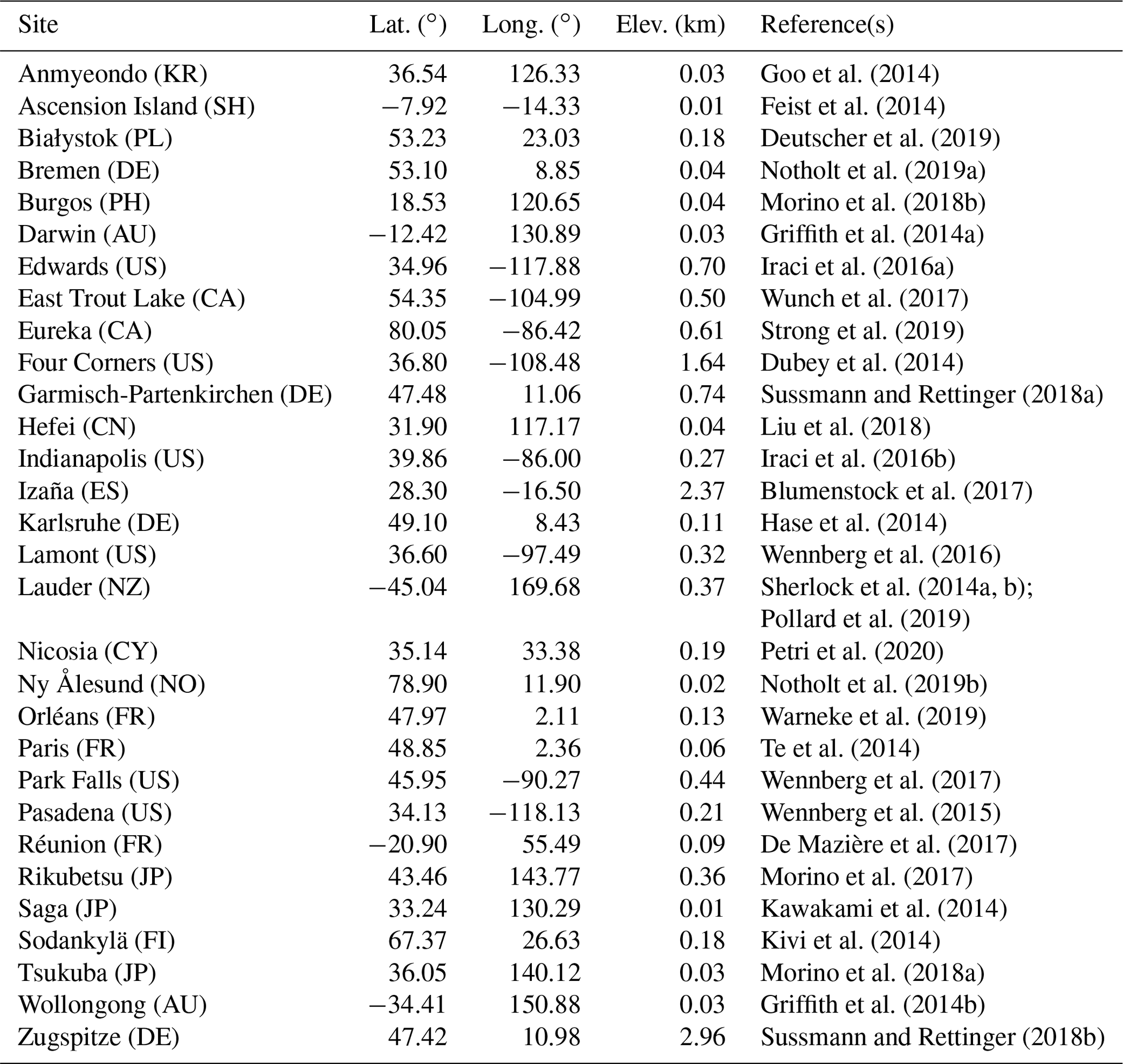
The same TCCON GGG2014 data are used for comparisons as in Noël et al. (2021), but now for the extended time period until the end of 2020. All involved TCCON stations and related references are listed in Table 1.
Goo et al. (2014)Feist et al. (2014)Deutscher et al. (2019)Notholt et al. (2019a)Morino et al. (2018b)Griffith et al. (2014a)Iraci et al. (2016a)Wunch et al. (2017)Strong et al. (2019)Dubey et al. (2014)Sussmann and Rettinger (2018a)Liu et al. (2018)Iraci et al. (2016b)Blumenstock et al. (2017)Hase et al. (2014)Wennberg et al. (2016)Sherlock et al. (2014a, b)Pollard et al. (2019)Petri et al. (2020)Notholt et al. (2019b)Warneke et al. (2019)Te et al. (2014)Wennberg et al. (2017)Wennberg et al. (2015)De Mazière et al. (2017)Morino et al. (2017)Kawakami et al. (2014)Kivi et al. (2014)Morino et al. (2018a)Griffith et al. (2014b)Sussmann and Rettinger (2018b)Table 1TCCON stations used in this study (update of similar table in Noël et al., 2021).
In addition to the validation with ground-based data we also include comparisons with other GOSAT data sets for XCO2 and XCH4, namely the ACOS v9r XCO2 product from NASA (Taylor et al., 2022); the full-physics and proxy products from the University of Leicester (UoL XCO2 and XCH4 FP v7.3, UoL XCH4 proxy v9.0; Cogan et al., 2012); the full-physics and proxy products from SRON (RemoTeC FP XCO2 and XCH4 v2.3.8, RemoTeC XCH4 proxy product v2.3.9; Butz et al., 2011); and the operational bias-corrected GOSAT XCO2 and XCH4 products from NIES v02.9x (Yoshida et al., 2013). The ACOS v9 data set is the “lite” product, downloaded in April 2020, which contains data up to end of 2019. We use only ACOS data with quality flag 0.
The retrieval used in this study is a three-step approach consisting of pre-processing, processing and post-processing. It uses as input the calibrated GOSAT/GOSAT-2 spectral radiances, independently for each polarisation direction. Since the retrieval method is essentially the same as the one described in Noël et al. (2021) for product version 1.0, we will describe in the following only the differences applied for the updated product version (v3.0; v2 was an unreleased internal version). Most relevant changes for the current product version were in the pre-processing and post-processing parts.
The computational speed could be slightly improved in v3.0 compared to v1.0. For GOSAT, the retrieval for one ground pixel is typically done within about 20 s, GOSAT-2 processing takes a few seconds more due to the additional fitting windows. Note that this time is for the simultaneous retrieval for all data products. Times for pre-processing and post-processing are negligible compared to the retrieval.
3.1 Pre-processing
The pre-processing step collects and prepares all data required for the processing. This step especially includes the measured GOSAT and GOSAT-2 spectra, as well as geolocation and matching meteorological and topographic information (from ECMWF ERA5 and GMTED2010). Furthermore, some initial filtering (especially for clouds) is performed. The cloud filtering method is based on the derivation of an effective albedo and a water vapour absorption filter from the spectral data as described in Noël et al. (2021). This makes use of the facts that clouds are usually bright and are located above the surface such that the amount of water vapour above the cloud is low.
For the new FOCAL products, two filter limits of the pre-processing have been relaxed to increase the final data yield: we now use a maximum solar zenith angle (SZA) of 90∘ and also latitudes up to ±90∘. In v1.0, both limits were set to 70∘. Note that these limits are applied for pre-processing; further filtering is done later during post-processing, depending on the different products (see Sect. 3.3). All other filtering (including the cloud filter) is unchanged compared to v1.0. The main difference in pre-processing to v1.0 is, therefore, that for v3.0 high latitudes are not necessarily filtered out before processing. This allows for more flexibility in the definition of product-specific post-processing filters by taking into account different sensitivities of each product. Furthermore, as mentioned above, we now use SLIMCO2 and SLIMCH4 data as a priori data for XCO2 and XCH4.
3.2 Processing
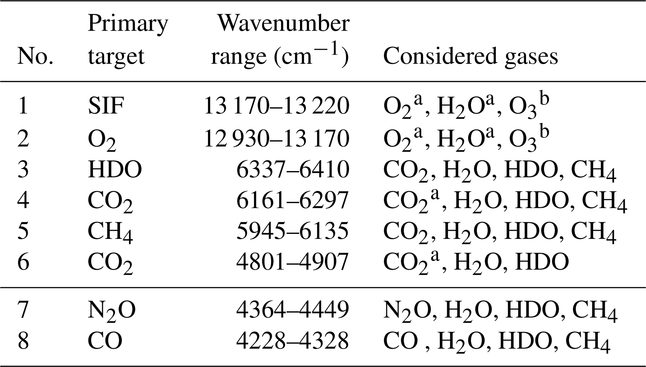
Both v1.0 and v3.0 processing versions use the FOCAL algorithm described in Reuter et al. (2017b). FOCAL is a full-physics retrieval method, which approximates scattering in the atmosphere by a single layer. With this, the forward model to simulate radiation can be expressed as an analytical formula, which allows for a high computational speed. The v3.0 updates to FOCAL include the use of a modified version of FOCAL, which assumes isotropic instead of Lambertian scattering at the scattering layer, and we also fit H2O in the NIR band (see Table 2).
Table 2Definition of GOSAT/GOSAT-2 spectral fit windows (same for S and P polarisation). Windows 7 and 8 are only available for GOSAT-2. Cross sections are from HITRAN2016 except for those marked with “a”, which are from ABSCO v5.1, and those marked with “b”, which are from Gorshelev et al. (2014) and Serdyuchenko et al. (2014).
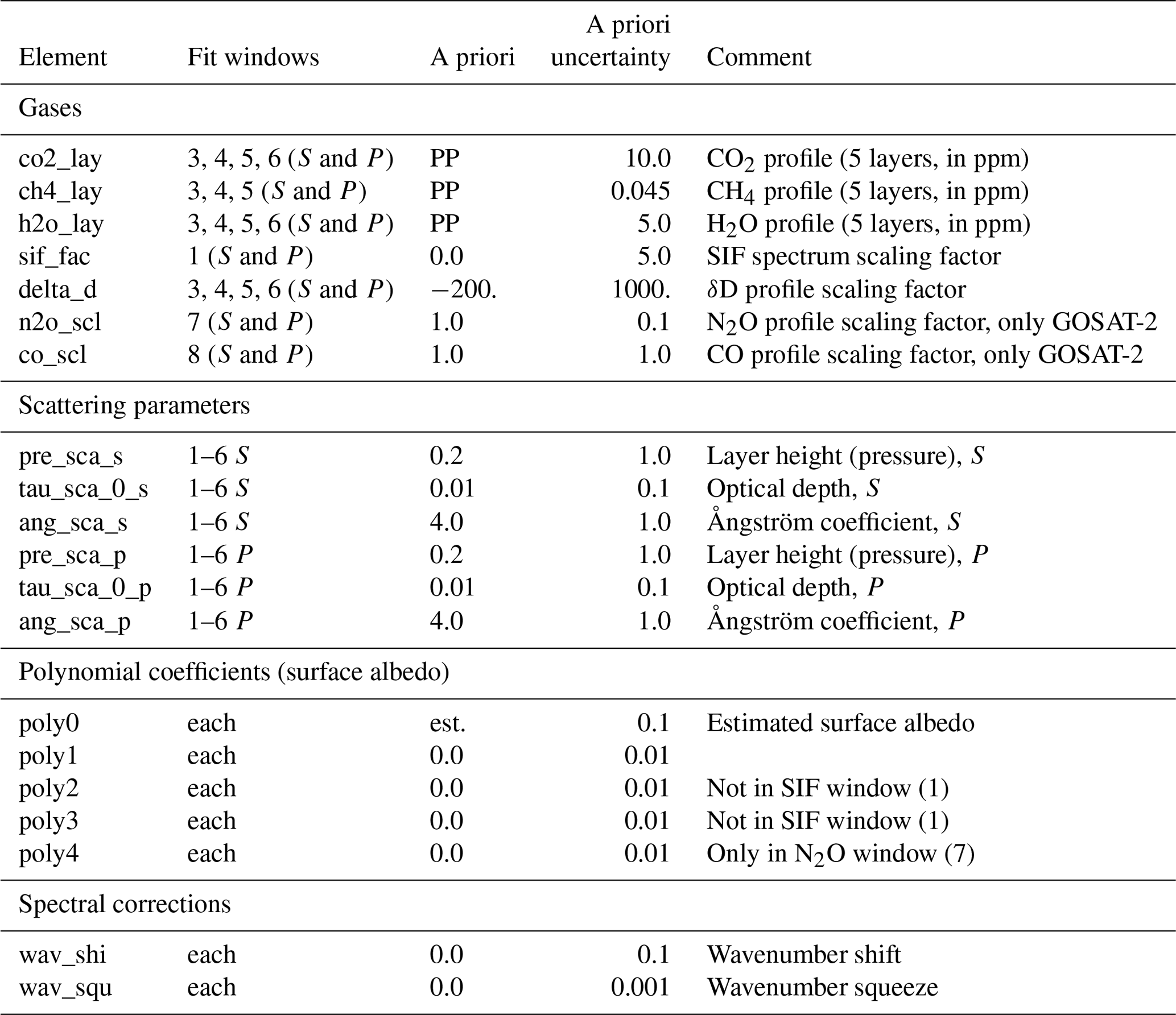
The FOCAL retrieval is based on an optimal estimation algorithm (Rodgers, 2000), taking as main input measured calibrated spectra and their uncertainties. The quantities to be retrieved are collected in the state vector, and secondary inputs to the retrieval algorithm are corresponding a priori values and their uncertainties in the form of an a priori error covariance matrix. The main output of the FOCAL retrieval is the values and uncertainties of the elements of the state vector. The state vector elements of v3.0 (see Table 3) are almost the same as in v1.0; however, we increased the degrees of the background polynomials to improve the fit residuals such that now all fitted polynomials are of degree 3 except for the small solar-induced fluorescence (SIF) windows where we use a degree of 1 and the XN2O window where a degree of 4 is used. The latter is done because the sensitivity of XN2O to surface effects turned out to be larger than for the other products. All quantities in the state vector are retrieved simultaneously. For CO2, CH4 and H2O, we derive profiles on five layers which are then converted to total column averages.
δD, XCO and XN2O are derived via scaling factors. The XCH4 proxy product is derived after the retrieval from these full-physics products (see below). In the case of GOSAT-2, all scattering parameters as well as methane, water vapour and δD are only fitted in windows 1 to 6 (i.e. those spectral ranges which are also available for GOSAT). This is done to provide consistent products for the two sensors.
As in v1.0, for GOSAT – but not GOSAT-2 – we compute a spectral correction factor to account for changes in the spectral calibration with time. In v3.0 the factor is obtained from the spectral difference of Fraunhofer lines in the solar irradiance and measured radiance in the SIF window, which is more stable than the least-squares fitting procedure used in v1.0. This new method only corrects for shifts on the scale of one spectral sampling interval (0.2 cm−1); this, however, is sufficient, as additional spectral shift and squeeze factors are determined in the later retrieval for both versions.
We also use a noise model to correct the uncertainties of the GOSAT and GOSAT-2 spectra estimated during pre-processing and consider possible forward model uncertainties in the retrieval. This noise model is the same as in v1.0, but we recomputed the parameters for all fitting windows based on an input data set consisting of 1 d per month in 2019 for both GOSAT and GOSAT-2. The resulting parameters are, however, similar for v1.0 and v3.0.
3.3 Post-processing
The main changes between v1.0 and v3.0 occur in the post-processing step. The overall concept of our new approach is that we tried to establish a generic, mostly automated, procedure that provides reproducible results and thus can be applied to all gases under consideration. However, it still allows for an optimisation for each product.
The following post-processing steps are in general applied to all products:
-
basic filtering,
-
quality filtering,
-
bias correction (for CO2 and CH4 only).
Note that, in contrast to v1.0, there is no longer a filter on the derived bias applied after the bias correction.
The XCH4 proxy product is computed during post-processing from
This means we normalise the retrieved full-physics XCH4 by the retrieved full-physics XCO2 (both without bias correction) and use as reference the a priori XCO2. Note that this is different to, for example, the SRON XCH4 proxy product (Wu et al., 2021), which is derived from a dedicated non-scattering retrieval using a different wavelength region (6045–6138 cm−1). The uncertainty of the proxy product is then determined via error propagation. The XCH4 proxy product is then treated in post-processing as the other products.
The general advantage of proxy products (see also Parker et al., 2011, 2020; Schepers et al., 2012) is that they are less sensitive to light-path effects like scattering. They therefore usually have a larger coverage. However, they usually depend on a model reference, which is in our case SLIMCO2 (see Appendix A). The uncertainty of the XCH4 proxy product is also larger than for the full-physics product, because it includes the uncertainty of the derived XCO2.
Table 3State vector elements and related retrieval settings. A priori values are also used as first guess. The “Fit windows” column lists the spectral windows (see Table 2) from which the element is determined; “each” means that a corresponding element is fitted in each fit window. A priori values labelled as “PP” are taken from pre-processing; “est.” denotes that they have been estimated from the background signal.
3.3.1 Basic post-processing filters
In contrast to v1.0, the basic filtering does not involve filtering based on external information, e.g. by using pre-described limits of scattering parameters or product uncertainties. This is no longer done as these fixed limits removed too many possibly valid data points, especially in the case of GOSAT-2.
Therefore, the basic filtering now only includes the filtering for good convergence (χ2 smaller than 2) and a maximum residual-to-signal ratio (RSR) as a function of the noise-to-signal ratio (NSR). This is done in the same way as for v1.0 (see Noël et al., 2021) but with the updated noise model parameters mentioned above. This part of the basic filtering is common for all products.
For GOSAT, the RSR filters for all fitting windows (1–6) are applied to all data products. In the case of GOSAT-2, for consistency, we also apply only the RSR filters for windows 1–6 to those products that are also available from GOSAT (i.e. XCO2, methane and water vapour products). For the other two GOSAT-2 products, i.e. XCO and XN2O, we only apply RSR filters from the NIR (windows 1 and 2, which contain the majority of the information related to scattering) and those windows where these gases are retrieved, namely window 8 for XCO and window 7 for XN2O. This is to avoid inadvertently filtering out a valid XCO2 measurement due to, for example, a bad XN2O fit (or vice versa).
In addition to this, we apply a filter on a maximum SZA of 75∘, because we cannot expect good data products at low solar illumination. This is a slightly higher limit than in v1.0, where all data above 70∘ were already filtered out during pre-processing. This SZA filter is applied for all products except for water vapour, because requirements for water vapour are not as strict as, for example, for XCO2. This is why we do not apply this strict filter already in pre-processing (where we only limit the SZA to 90∘; see above).

3.3.2 Quality filtering
The quality filtering is product-specific, but it follows the same strategy for each target gas. In general, we perform independent filtering for water and land surfaces. The final data product contains only the filtered data. The filtering out of low-quality data was done in v1.0 by a random forest filter. However, as explained in Noël et al. (2021), the performance of this method was not ideal as it filtered out fewer data than expected, i.e. less data were filtered out than were marked as “bad” during the training of the random forest filter. Therefore, we replaced this filtering for v3.0 with a filter procedure that has already been successfully used in OCO-2 retrievals; details can be found in Reuter et al. (2017a). This procedure is based on a minimisation of the local variance. This is done by computing, for a subset of the data, the variance of the difference between the retrieved quantity and its median on a 15∘×15∘ grid. Based on this subset, we check which variables from a given list of the candidate variables perform best in reducing the local variance when removing data corresponding to the highest or lowest 1 % of each variable. This action defines a new upper or lower limit for this variable. We repeat this until a prescribed amount of data are removed. The output of this procedure is a list of “best” variables and their new filter limits. This subset has been generated from data of 2019 for GOSAT and GOSAT-2, to which the basic quality filter as described above has been applied. Note that – in contrast to v1.0 – this subset no longer depends on the reference database used in the bias correction. A general problem with this filtering method is that it tends to filter out values from regions with higher noise, which might result in reduced coverage at higher latitudes if too many data are to be filtered out. Therefore, we apply this filtering in two steps. First, using the variance filter method, we determine limits for only the scattering optical depth parameters contained in the state vector in order to filter out a set percentage (Pτ) of the data. After applying this filter, we further reduce the number of data by another percentage (PV) using the variance filter method again but now for an extended list of possible filter candidates. This list of variables has been largely reduced compared to v1.0. It now only comprises results from the retrieval, namely the uncertainties (but not values) of the retrieved target species, χ2, scattering parameters and their uncertainties, the polynomial coefficients and their uncertainties, wavelength shift/squeeze and their uncertainties, and surface roughness. We explicitly no longer include geolocation/viewing geometry parameters or surface elevation to avoid cases where data are filtered out due to, for example, a specific geographical region. The retrieved CO2 gradient at the surface is also not used anymore, as this might result in filtering out scenes with too high CO2 in the boundary layer close to a point source. However, because of the large number of fitting windows this still leaves a list of about 200 possible parameters. To reduce this to a reasonable number, we run this variance filter twice: first with the full list and then with only the 10 best parameters. This number (10 parameters) is only an upper limit, which has been chosen by checking that adding more parameters does not further reduce the variance significantly. Depending on the relevance of individual quantities, even fewer parameters are needed in some cases.
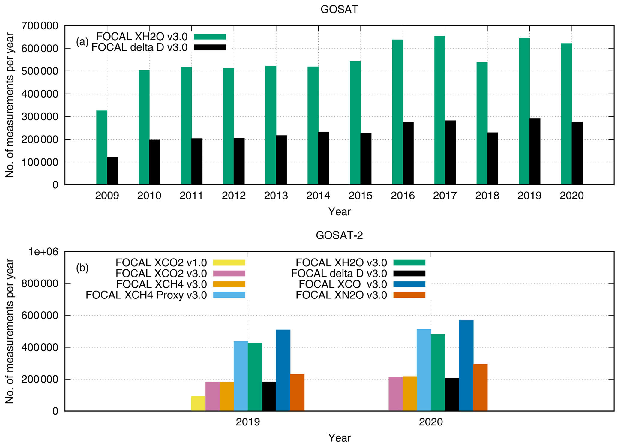
Figure 2Number of FOCAL GOSAT and GOSAT-2 data as a function of time. (a) GOSAT FOCAL XH2O and δD; (b) GOSAT-2 FOCAL products.
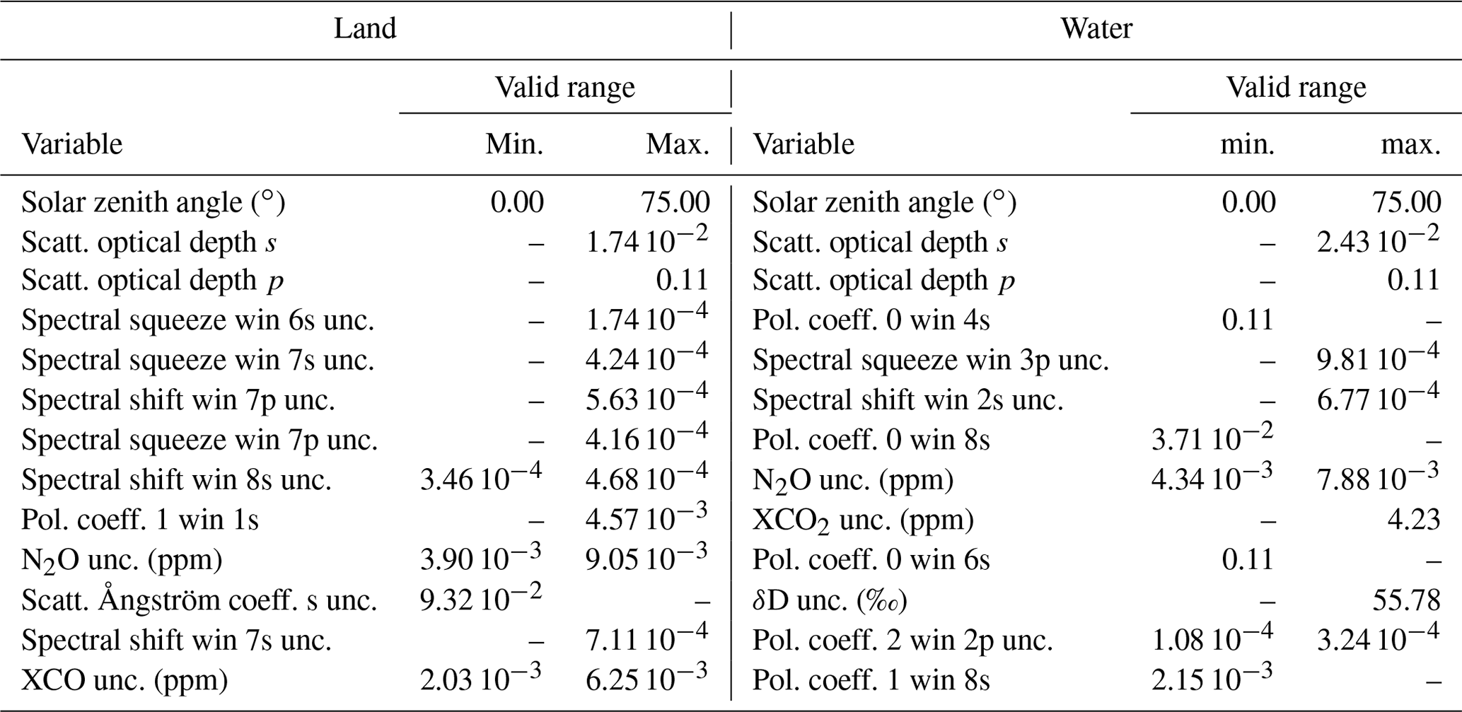
The choice of the number of data to be filtered out is – as always – a trade-off between the remaining number of data points and data quality. For the v3.0 data, we determined suitable numbers for Pτ and PV by looking at the resulting data quality (maps and validation) for different settings. As with the SZA filter, the optical depth filter is not applied for each product. We use the same values for GOSAT and GOSAT-2; these are listed in Table 4. The final set of selected filter variables and their limits is specific to each product, surface and instrument. They are given in Appendix A in Tables A1 to A12.
Table 4Filter settings for all products; “–” denotes that no limit is applied.

Note that the minimisation of the variance is done for the whole test data set, i.e. a year of global data. Small, local sinks or enhancements should have no impact here, as long as there is no clear correlation between, for example, a filter variable and the retrieved value or the geolocation. This is why we only use a very restricted list of possible variables.
3.3.3 Bias correction
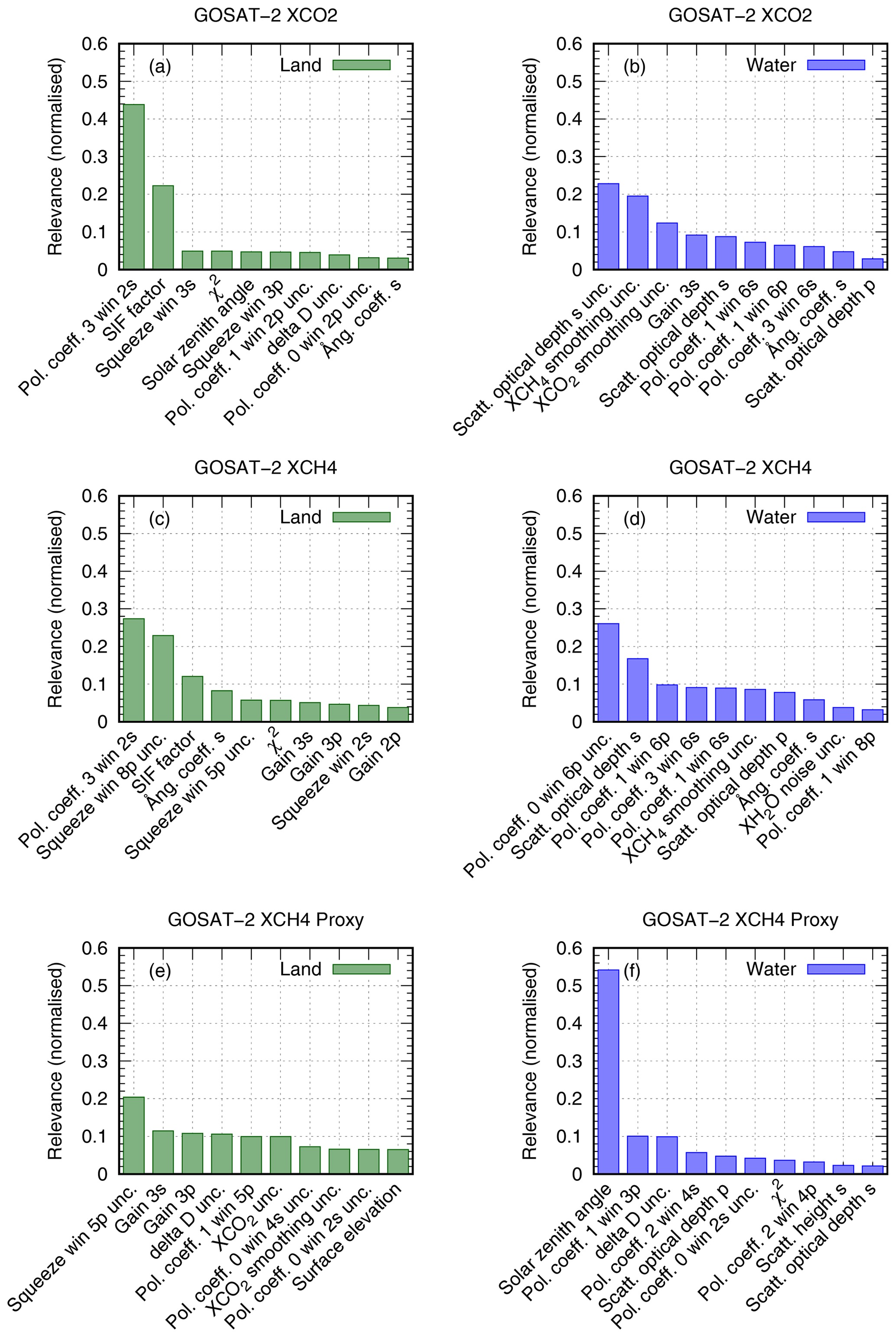
After filtering data as described above, we apply a bias correction to XCO2 and the XCH4 full-physics and proxy products. The overall procedure is the same as described in detail in Noël et al. (2021). The bias correction is based on a random forest regression using, as for v1.0, the 10 most relevant parameters and a random forest database as input. These have been determined as described in Noël et al. (2021), using as input the variance-filtered test subset of data as mentioned above and a reference database giving the “true” XCO2 and XCH4. This reference database has been generated from a subset of daily SLIMCO2 and SLIMCH4 data (see Appendix A) for 2019, which agree within ±0.5 ppm for XCO2 and ±10 ppb for XCH4 with corresponding TCCON data. The best parameters have been chosen from essentially the same list of candidate variables used in the variance filter but now extended with surface elevation and type, solar zenith angle, viewing zenith angle, continuum signal, and flags for quality and instrument gain. The final choice of bias correction parameters and their relevance is shown in Fig. A7 for GOSAT and Fig. A8 for GOSAT-2 (see Appendix B).
We also perform a correction of the retrieved XCO2 and XCH4 uncertainties (ΔXretr) via a linear function:
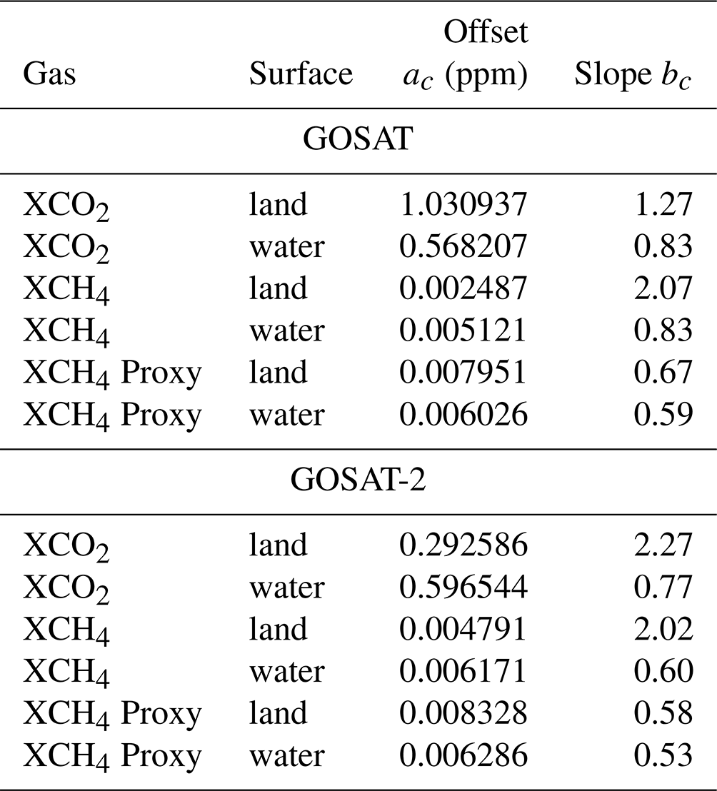
ΔX is the corrected uncertainty with X being either XCO2 or XCH4. The coefficients ac and bc of this function (see Table 5) are determined in a similar way as described in Noël et al. (2021) by comparing the scatter of the data relative to a truth with the retrieved uncertainty, but instead of TCCON data we now use data from the SLIMCO2/SLIMCH4 reference database as true values.
All GOSAT data (from 2009) and GOSAT-2 data (from 2019) until the end of 2020 have been processed. Figs. 1 and 2 show the final number of valid FOCAL data as a function of time for the different products. The numbers are different for each product because of the individual filtering (see above). For comparison, the numbers for the v1.0 XCO2 products are also shown. Fig. 1a compares the number of yearly GOSAT FOCAL XCO2 data with other available GOSAT data products from SRON, the University of Leicester (UoL), NIES and the NASA ACOS v9 product. A similar comparison is shown in Fig. 1b for XCH4 full-physics and proxy products. The resulting amount of data for the GOSAT FOCAL water vapour products is shown in Fig. 2a.
The yield of valid FOCAL products was improved in v3.0 compared to v1.0. The number of valid FOCAL XCO2 and methane results exceeds those of all other GOSAT data sets. Note that the increase in data yield from v1.0 to v3.0 is actually larger over water (about 60 % for 2019) than over land surfaces (about 30 % for 2019). The main reason for this increase is the improved post-processing quality filtering procedure and – especially for water vapour – also relaxations in the latitudinal and solar zenith angle filtering during pre-processing.
In general, the number of GOSAT data increases for all products with time, with typically more data after 2015. As discussed in Noël et al. (2021), this is related to optimised GOSAT operations especially resulting in more data over water.
In principle, GOSAT-2 should provide more valid data than GOSAT, because GOSAT-2 uses an “intelligent pointing” procedure to avoid cloudy scenes. However, although the total number of GOSAT-2 FOCAL products (see Fig. 2b) was also improved, it is still lower than for GOSAT. This is because a larger fraction of data are already removed during the basic filtering due to larger residuals/less convergence. This hints at possible issues with the radiometric calibration or an incomplete instrument model used by FOCAL, neglecting important instrument features, e.g. currently unconsidered effects of remaining polarisation sensitivities of the instrument.
4.1 Global maps
For each of the different data products, an example map comprising a mean for April 2019, gridded to 5∘× 5∘, is shown in Figs. 3 to 8 for GOSAT and GOSAT-2. In all maps, grid points that were only based on a single measurement have been omitted to avoid outliers. The spatial patterns of XCO2, methane, water vapour and δD look very similar for GOSAT and GOSAT-2. GOSAT-2 data show in general fewer gaps over the oceans but with smaller latitudinal coverage. The latter is due to the currently applied RSR filtering for GOSAT-2, which especially removes data over water surfaces. Note that over the year the spatial range of valid data varies according to solar illumination conditions.
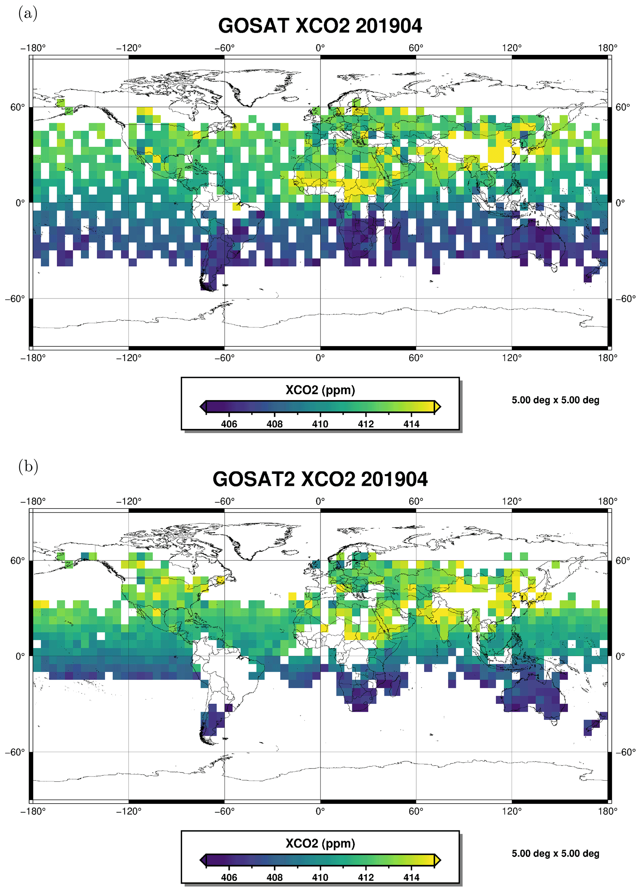
Figure 3Maps of gridded XCO2 data for April 2019: (a) GOSAT; (b) GOSAT-2.
The XCO2 data show higher values in the Northern Hemisphere than in the Southern Hemisphere as expected during springtime. This is because plants absorb more XCO2 during growing season (i.e. hemispheric summer and autumn).
For methane, the known source regions in the USA, Africa and Asia are clearly visible, as well as the inter-hemispheric gradient. The spatial coverage of the proxy product is much larger than for the full-physics product, especially at higher latitudes. This is due to the relaxed filtering for the proxy product.
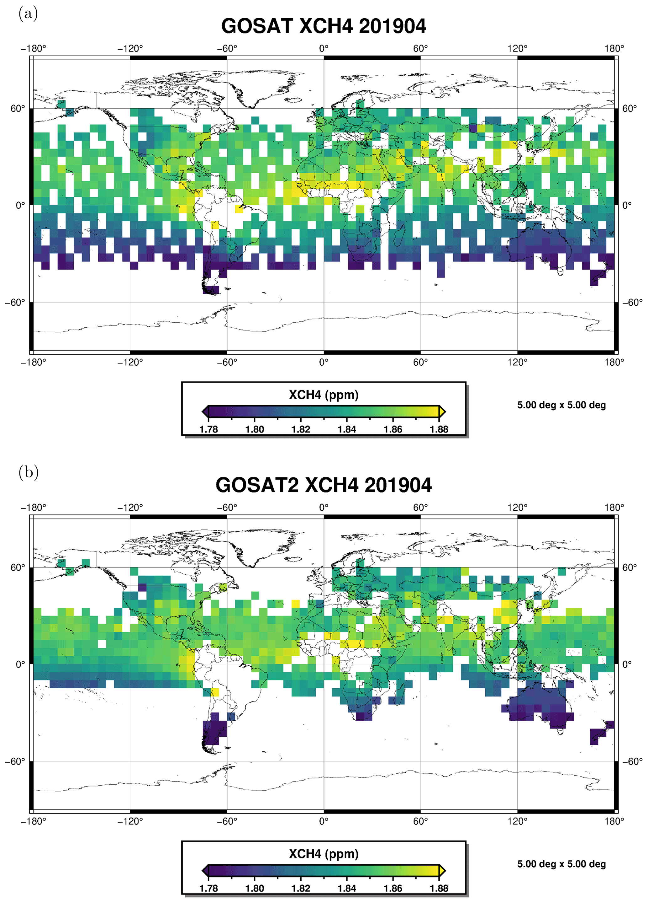
Figure 4Maps of gridded XCH4 data for April 2019: (a) GOSAT; (b) GOSAT-2.
Water vapour (XH2O) also shows the expected behaviour: large values in the tropics and lower values at higher latitudes. The observed spatial distribution of δD is in line with the maps shown in Frankenberg et al. (2013). All δD values are in the expected range (about 0 to −300 ‰); they also decrease from the tropics to higher northern and southern latitudes. This is because water vapour generated in the tropics by strong evaporation is transported to higher latitudes, during which the heavier HDO decreases more rapidly via precipitation than H2O.
For GOSAT-2, there are also data for carbon monoxide (XCO) and XN2O. In the XCO map the expected source regions in China, Indonesia and Africa (fossil fuel combustion, biomass burning) are apparent over the otherwise quite smooth and constant background. The transport of XCO from the equatorial African fire regions to the west over the Atlantic Ocean due to the trade winds is clearly visible, as is some transport from Asia to the Pacific.
The XN2O product shows an overall decrease of the background XN2O from the tropics to higher latitudes on the order of 15 ppb. Such gradients were also observed by the IASI (Infrared Atmospheric Sounding Interferometer) instrument on Metop (Barret et al., 2021); however, we see larger differences. This could be related to the sampling of the XN2O data.
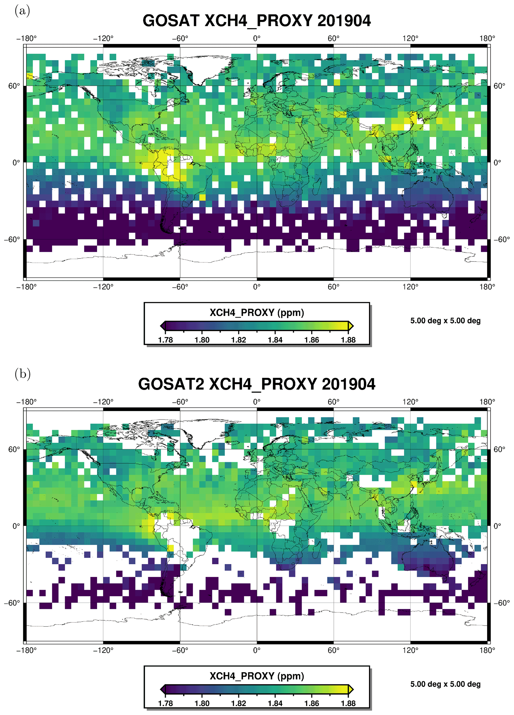
Figure 5Maps of gridded XCH4 Proxy data for April 2019: (a) GOSAT; (b) GOSAT-2.
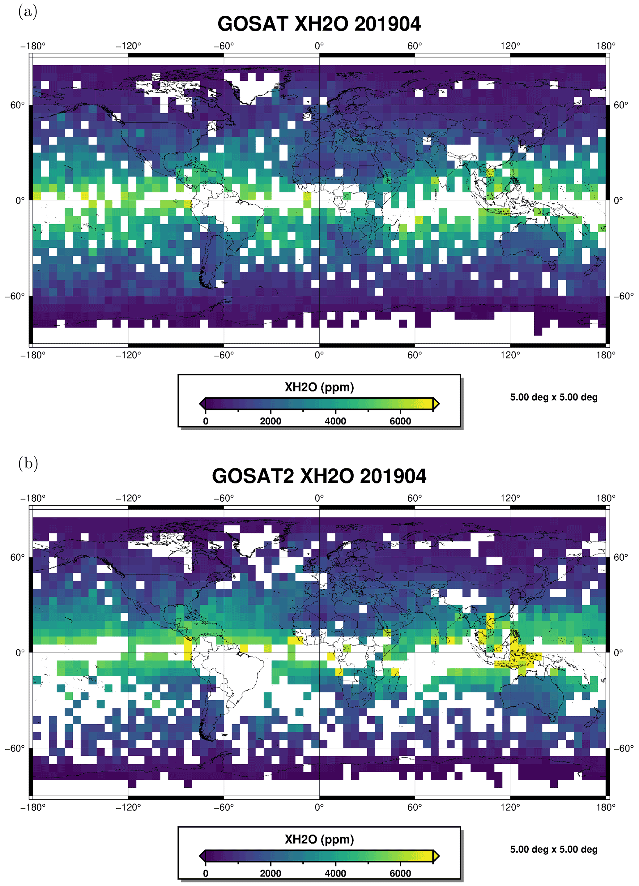
Figure 6Maps of gridded XH2O data for April 2019: (a) GOSAT; (b) GOSAT-2.

Figure 7Maps of gridded δD data for April 2019: (a) GOSAT; (b) GOSAT-2.

Figure 8Maps of gridded GOSAT-2 data for April 2019: (a) XCO; (b) XN2O.
Furthermore, the IASI data shown in Barret et al. (2021) refer to the mid-troposphere over the ocean only, whereas the GOSAT-2 FOCAL data are total column averages over all surfaces. The latitudinal XN2O gradient can, in principle, be explained by the variation of the tropopause height. As most of the XN2O is contained (and well mixed) in the troposphere, the total column average is larger in the tropics (where the tropopause is high) than at higher latitudes. We also see increased XN2O over central Africa. This is also visible in IASI data and probably related to convection (see Ricaud et al., 2009).
4.2 Time series
Time series of all GOSAT FOCAL data products for different latitudinal regions are depicted in Fig. 9. These plots show the expected temporal behaviour: a seasonal cycle is visible in all data sets; amplitudes and/or phase differ for northern and southern latitudes with usually more variability in the north.
The GOSAT FOCAL XCO2 results are shown in Fig. 9a. The overall increase of XCO2 from around 380 ppm in 2009 to about 415 ppm in 2020 is clearly visible, as well as an overlaying seasonal variation, which is most pronounced in the Northern Hemisphere with a minimum in summer due to vegetational growth. In the Southern Hemisphere, the seasonality of XCO2 is shifted by 6 months but much lower since there are less land masses than in the north. The global variation is very similar to the tropical one.
The methane full-physics and proxy products show a similar temporal variation with increasing XCH4 due to larger anthropogenic contributions (about 10 ppb per year, which is in line with recent annual changes from NOAA ground-based measurements; see https://gml.noaa.gov/ccgg/trends_ch4/, last access: 11 January 2022). Small differences between the average XCH4 full-physics and the proxy products can be explained by the broader spatial coverage of the proxy product.
For water vapour (XH2O), the seasonal cycles in the Northern Hemisphere and Southern Hemisphere are shifted by about 6 months, in line with the seasonal shift of the intertropical convergence zone (ITCZ). On the global scale, these seasonal variations largely average out. Some change in the seasonal cycle of XH2O is seen after 2015. This is probably related to the increased number of GOSAT data (especially over ocean) after 2015 (see Fig. 1), which changes the sampling. Taking this into account, no clear trend is visible in the GOSAT water vapour data from 2009 to 2020, although there is some indication for a slow increase with time. This is in line with results from other data sets (see e.g. Borger et al., 2022, and references therein).
Average values of δD vary between about −180 ‰ and −120 ‰. As for water vapour, seasonal variations are small in the global average, but year-to-year variations in the seasonal cycle are larger for δD. Especially note that the peaks in July 2012 in the Southern Hemisphere and in December 2018 in the Northern Hemisphere are due to very few data in these regions in these months.
The GOSAT-2 time series (see Fig. 10) show similar temporal variations to the GOSAT data, but of course, they only cover the years 2019 and 2020.
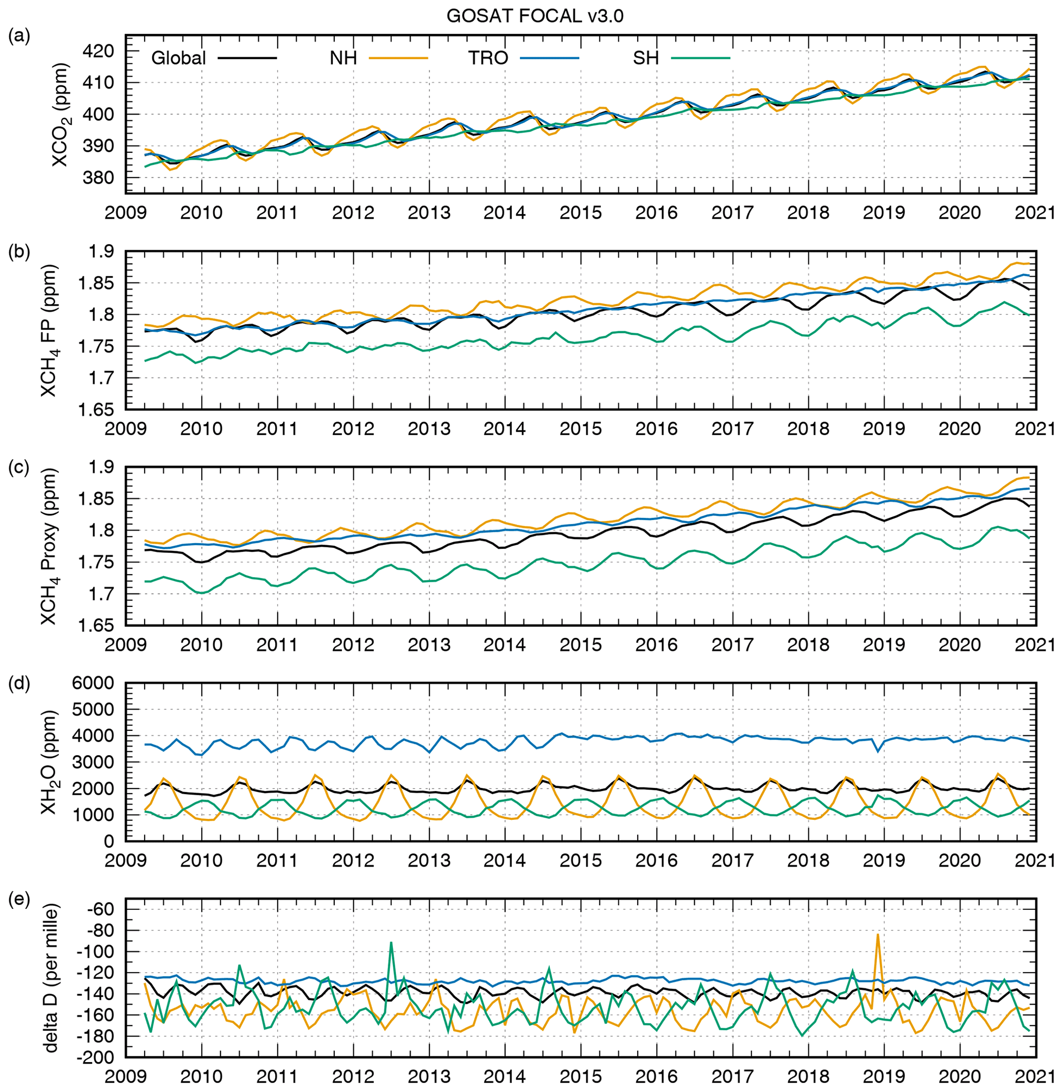
Figure 9GOSAT time series. NH = Northern Hemisphere (> 25∘ N). TRO = tropics (25∘ S–25∘ N). SH = Southern Hemisphere (< 25∘ S). (a) XCO2; (b) XCH4 full-physics product; (c) XCH4 proxy product; (d) XH2O; (e) δD.
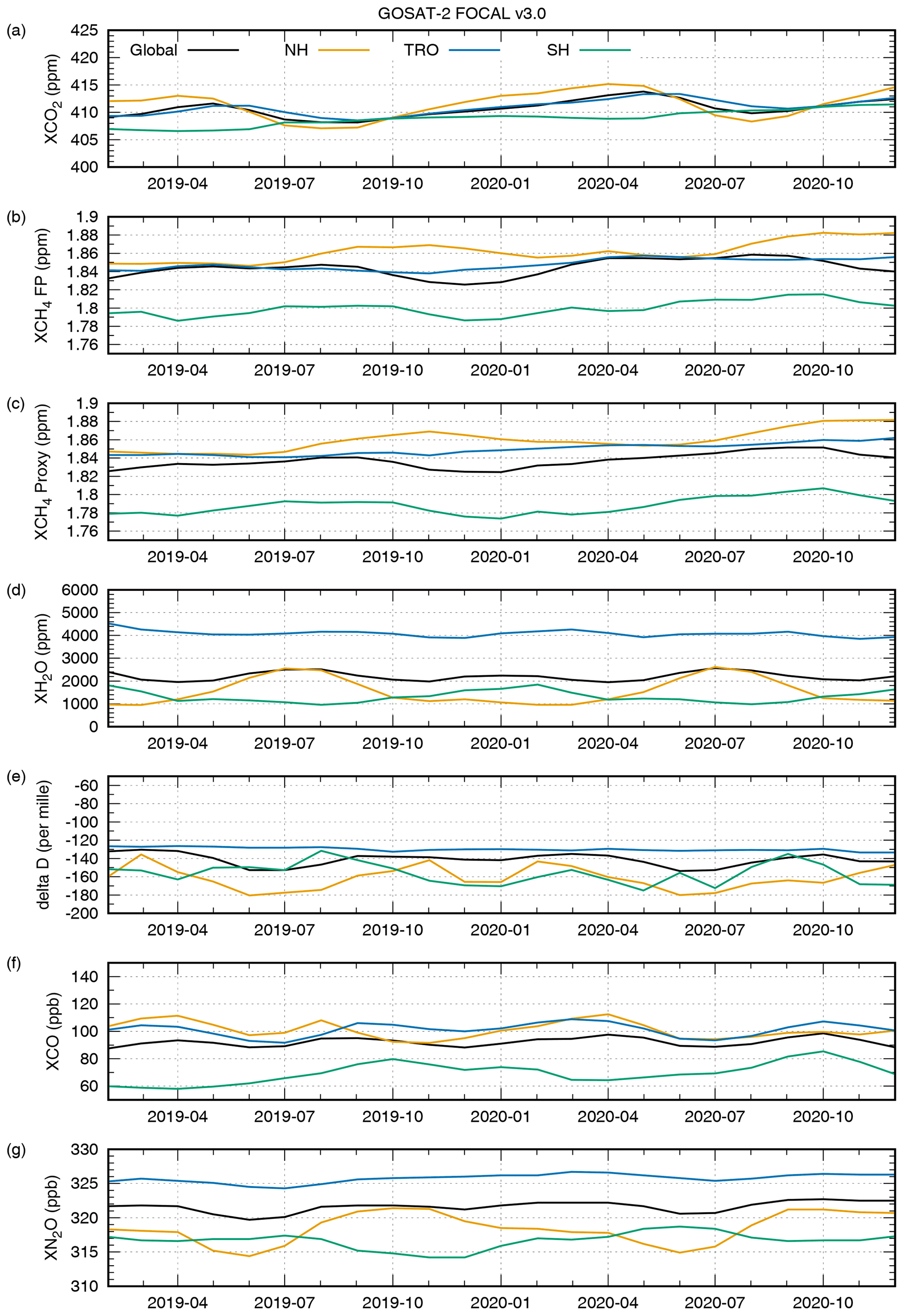
Figure 10GOSAT-2 time series. NH = Northern Hemisphere (> 25∘ N). TRO = tropics (25∘ S–25∘ N). SH = Southern Hemisphere (< 25∘ S). (a) XCO2; (b) XCH4 full-physics product; (c) XCH4 proxy product; (d) XH2O; (e) δD; (f) XCO; (g) XN2O.
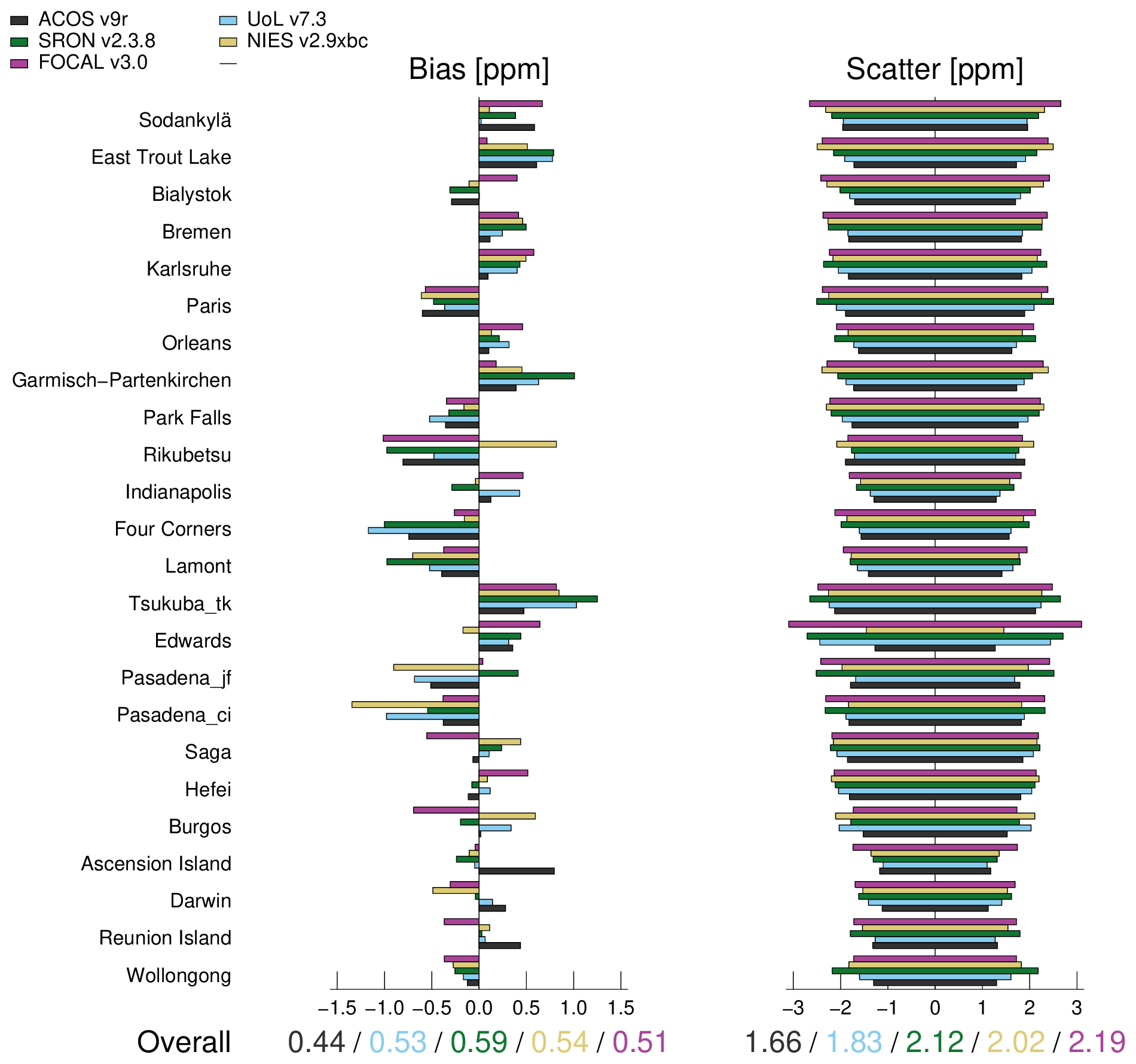
Figure 11Overview of comparison results between different GOSAT XCO2 products and TCCON data: scatter and bias for different TCCON stations. Note that the mean station bias has been subtracted to better illustrate the local station differences. See Table 6 for a summary of all TCCON validation results.
Across different latitudes, GOSAT-2 XCO shows similar values and seasonal variations, except in the Southern Hemisphere where XCO is on average about 30 ppb lower than in the Northern Hemisphere, probably because most sources are around the Equator or in the Northern Hemisphere extra-tropics.
The GOSAT-2 XN2O also shows some seasonal variations of up to about 8 ppb peak-to-peak. However, this seasonality is at least partly a sampling effect. The background XN2O, as shown in Fig. 8b, comprises larger values in the tropics than at higher latitudes. Because of the varying latitudinal coverage of GOSAT-2 ocean data throughout the year, the regions outside the tropics are not covered during all seasons, which introduces an apparent variation in the averages. This effect in principle applies to all data, but it is especially pronounced for XN2O, for which other spatial variations are low. In the tropics, the XN2O data are always high, and the variations are much smaller. In fact, we see a slight increase in XN2O of about 1 ppb per year, which is about what is expected from ground-based measurements (see growth rate plots on the NOAA Global Monitoring Laboratory website; https://gml.noaa.gov/hats/combined/N2O.html, last access: 30 June 2021). This result is also in line with IASI data (Barret et al., 2021).
4.3 TCCON comparisons
To assess the quality of the data, for each GOSAT and GOSAT-2 FOCAL product we perform a comparison with TCCON data using the same procedure as in Noël et al. (2021); see also Reuter et al. (2020) and Reuter and Hilker (2022) for details.
For most gases, we also use the same collocation criteria: a maximum time difference of 2 h, a maximum spatial distance of 500 km and a maximum surface elevation difference of 250 m between satellite and ground-based measurement. However, for water vapour and carbon monoxide these limits are reduced to 1 h time difference and 150 km spatial distance to account for their higher variability. We only include stations with a minimum of 50 data points.
For XCO2 and XCH4, we also perform comparisons with other available GOSAT products from SRON, the University of Leicester, NASA (ACOS v9) and NIES.
From the comparisons, we derive the following main quantities (related formulas are given in Reuter and Hilker, 2022):
-
The first is mean station bias, defined as the mean of all biases at each station; this can be interpreted as a global offset to all stations.
-
The second is station-to-station bias, defined as the standard deviation of the individual station biases. This can be interpreted as regional bias.
-
The third is mean scatter, defined as the square root of the mean of the variances at each station. This is a measure for the single sounding precision.
-
And the fourth is seasonal bias, defined as the standard deviation (rms) of the seasonal variation of the difference FOCAL–TCCON at each station. This is equivalent to a temporal bias.
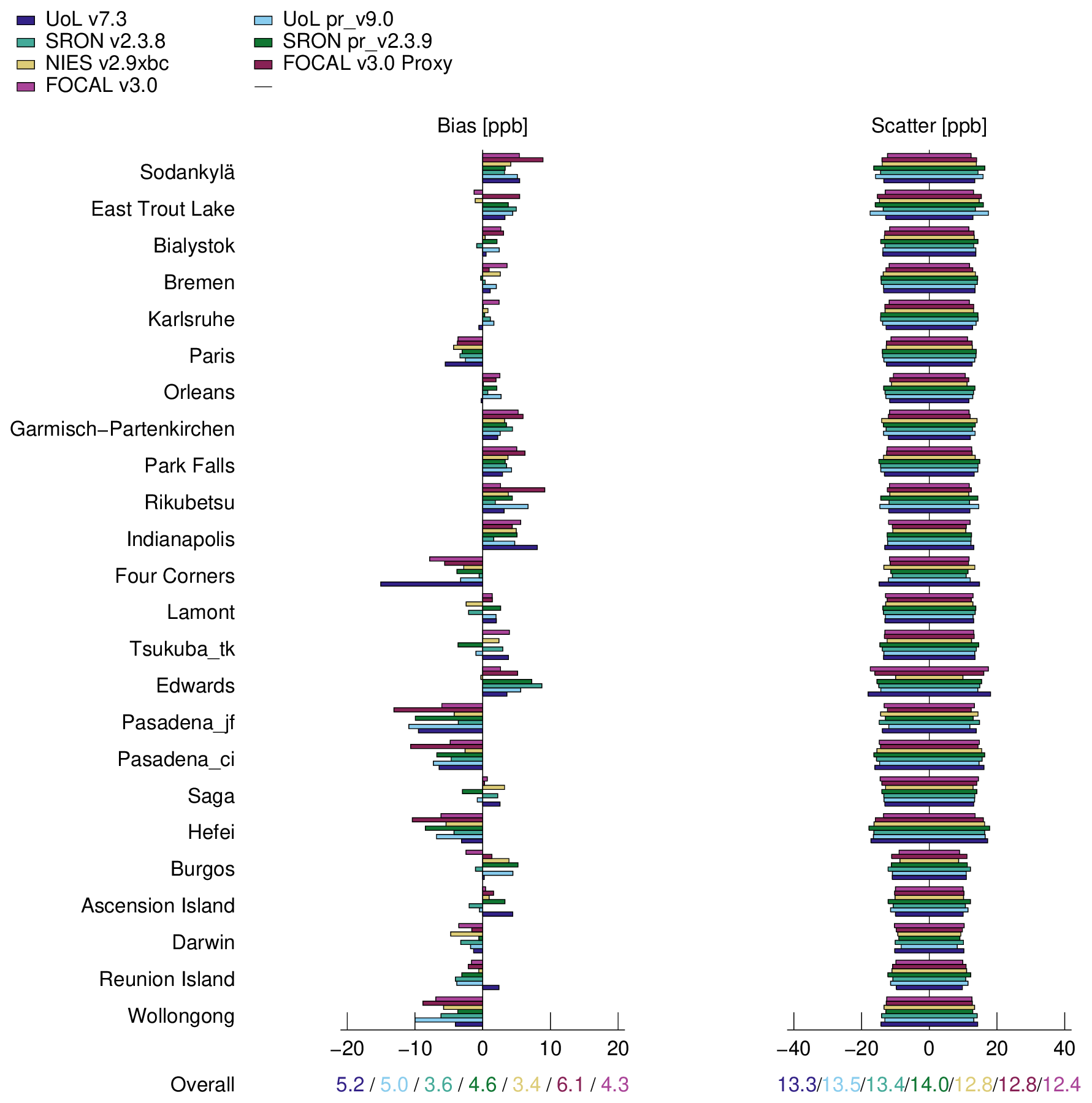
Figures 11 and 12 show the results from the TCCON validation for all GOSAT XCO2 and XCH4 (full-physics and proxy) products from the different retrievals. The validation for these products was performed using the same subset of stations for all data products of each gas, which allows for a direct comparison of the results. In addition, Figs. 13 and 14 show the TCCON validation results (bias and scatter) for each of the FOCAL v3.0 GOSAT and GOSAT-2 products (including the FOCAL data from Figs. 11 and 12). We also use here the same subset of stations for the GOSAT-2 XCH4 full-physics and proxy products. Example time series for the TCCON station Lamont (USA) are shown in Figs. 15 and 16. This station was selected as it provides good temporal coverage of TCCON data also for the GOSAT-2 time frame (2019–2020). All results of the comparisons are summarised in Table 6.
Table 6Results from TCCON comparisons. Nstations denotes the number of TCCON stations involved in the comparison, Ndata is the number of co-located data points. All products are full-physics products except for those marked as “Proxy”.
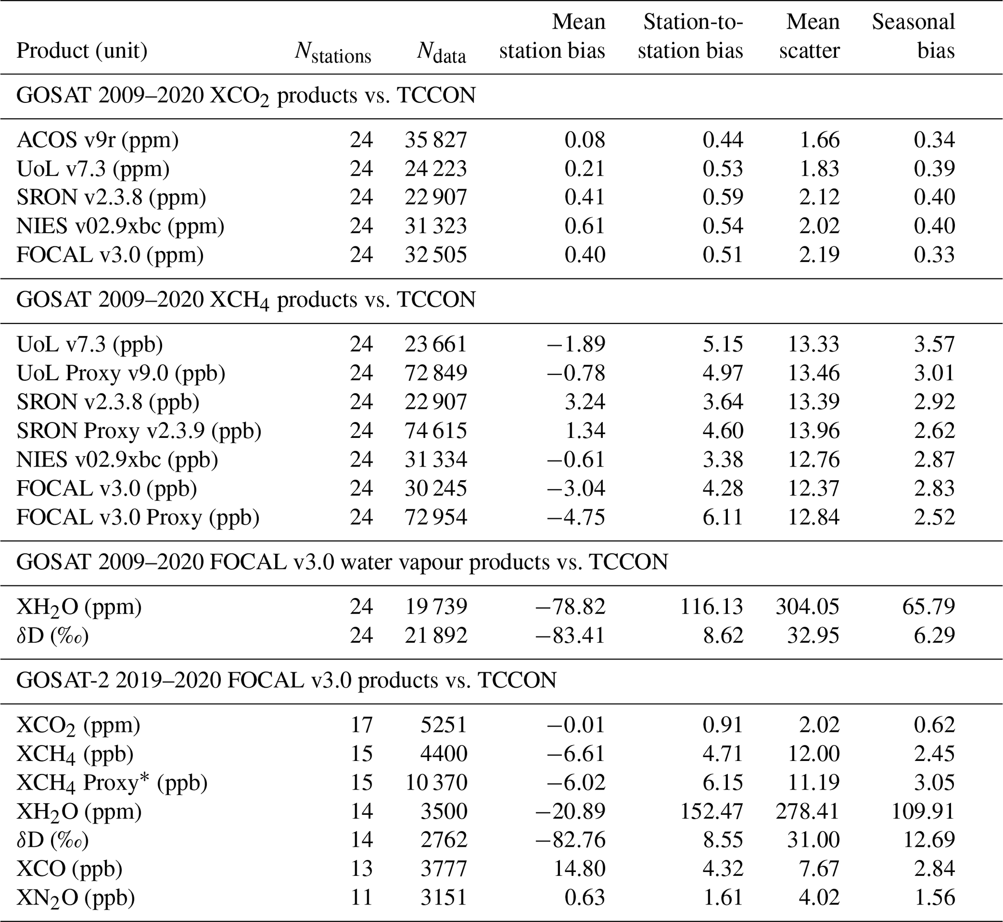
∗ XCH4 Proxy validated together with full-physics product, i.e. for same subset of TCCON stations.
The mean station bias is mainly given for reference, because it is usually not relevant for applications that are only interested in the spatial and temporal gradients of the gas (like for XCO2). The quantities station-to-station bias, seasonal bias and mean scatter are more important as they describe the quality of regional and/or temporal gradients, which are, for example, needed to quantify potential sources and sinks. The seasonal bias is derived from a trend model fit; therefore, the corresponding values for GOSAT-2 are less reliable, because the time interval is only about 2 years. The number of stations and data points used in the comparison depend on the different products, the collocation criteria and the length of the time series. Therefore, there are many fewer collocations for GOSAT-2. The XCH4 proxy products, as well as the XH2O and XCO products, have the largest number of collocations because of the relaxed filtering.
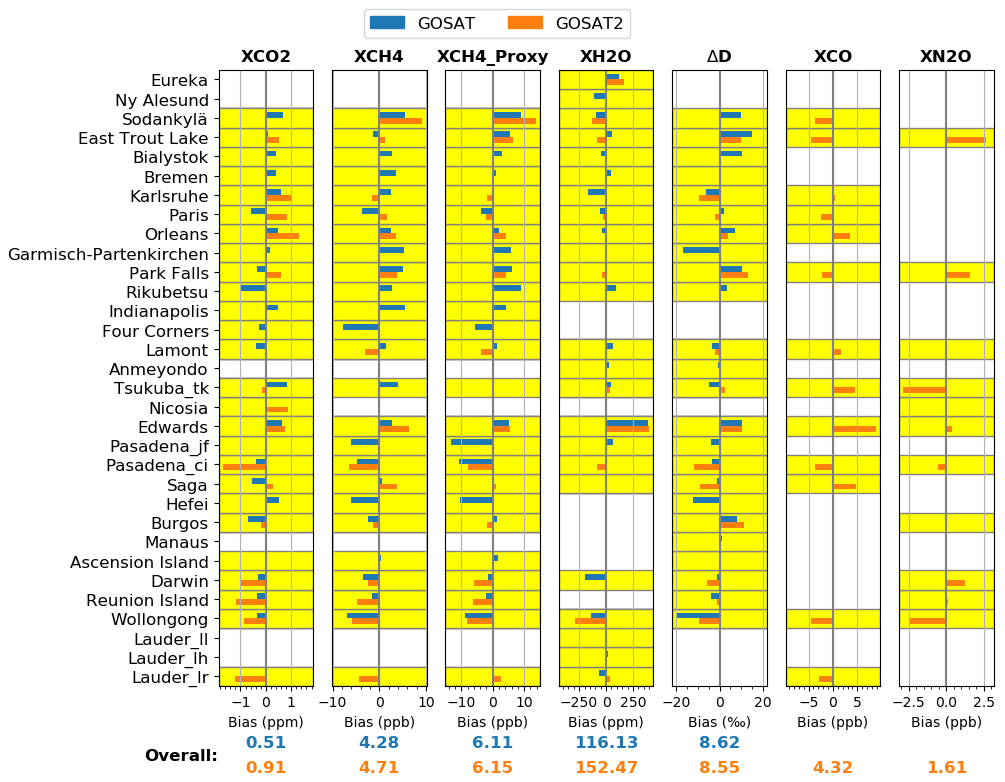
Figure 13Bias of FOCAL data products for GOSAT (blue) and GOSAT-2 (orange) at different TCCON stations. Involved stations for each product are marked by a yellow background. Note that small biases (close to zero) may not be visible in the plot. The mean station bias has been subtracted to better illustrate the local station differences. See Table 6 for a summary of all TCCON validation results.
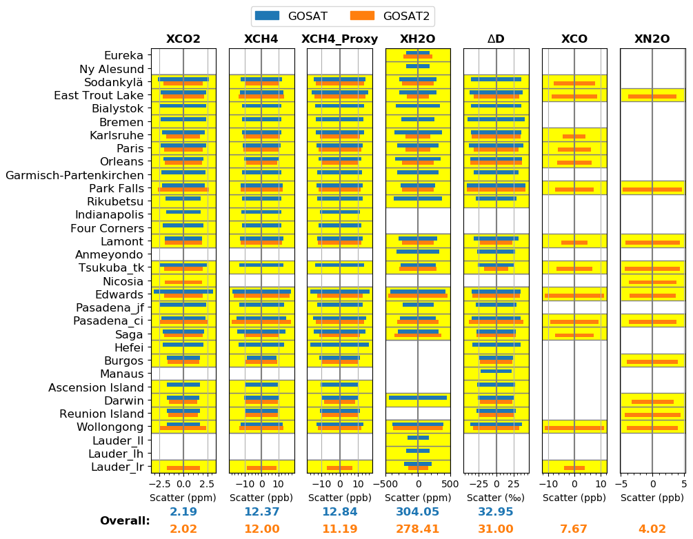
Figure 14Scatter of FOCAL data products for GOSAT (blue) and GOSAT-2 (orange) at different TCCON stations. Involved stations for each product are marked by a yellow background. See Table 6 for a summary of all TCCON validation results.
4.3.1 XCO2 results versus TCCON
For GOSAT FOCAL v3.0, the XCO2 station-to-station bias is 0.51 ppm, and the mean scatter is 2.19 ppm, as given by the pink numbers at the bottom of Fig. 11 and in Table 6.
While the bias is slightly reduced, the scatter is slightly larger than for v1.0 (0.56 ppm, 1.89 ppm; see Noël et al., 2021). This higher scatter is still acceptable, noting the increased number of data points, which always increases the scatter, and an estimated 1σ TCCON uncertainty of 0.4 ppm for XCO2 (Wunch et al., 2010). Note that this relation between scatter and number of data points is due to the filtering, which is based on reducing the local variance by removing data points (see above). The FOCAL values are also in quite good agreement with those from the other data sets but still do not reach the low bias and scatter of the NASA ACOS v9 product (0.44 and 1.66 ppm) as given in dark grey colour at the bottom of Fig. 11.
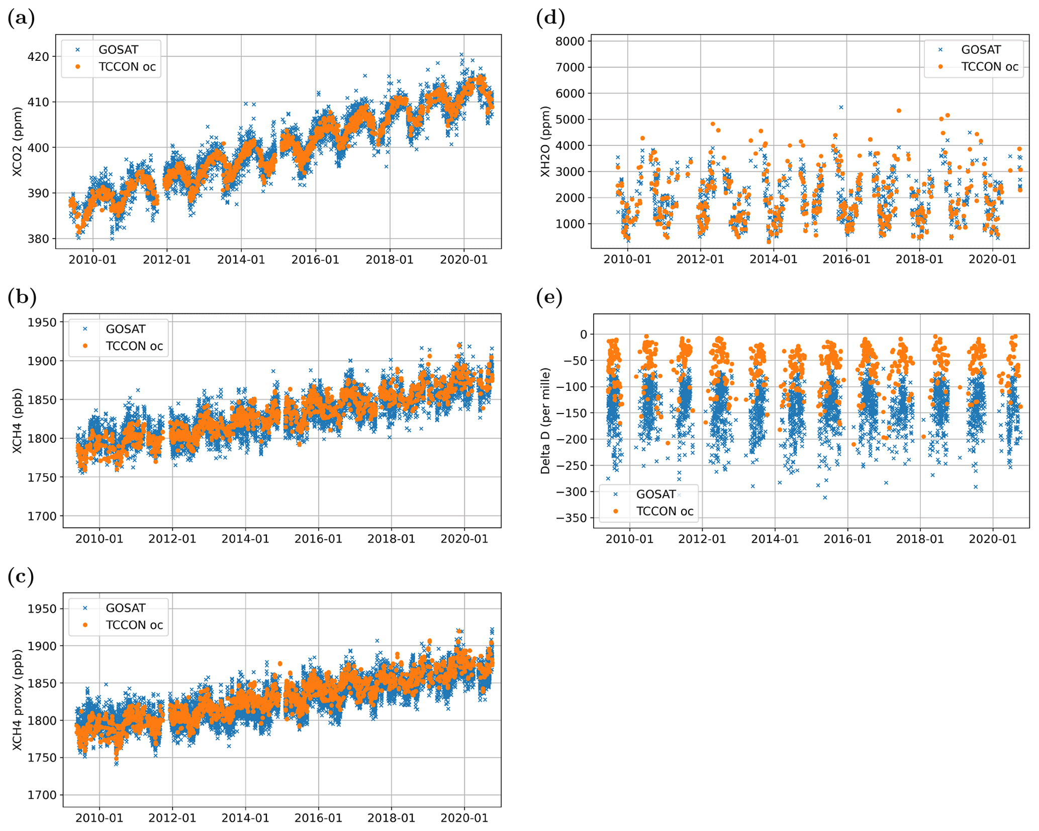
Figure 15Example time series of TCCON and GOSAT FOCAL data at Lamont (station code oc). (a) XCO2; (b) XCH4 full-physics product; (c) XCH4 proxy product; (d) XH2O; (e) δD.
The GOSAT-2 XCO2 comparison results for v1.0 were considered less reliable because of the shortness of the time series (less than 1 year). For v3.0, we now have almost 2 years of data and, due to the updated product version, also a higher data yield, which results in almost 10 times more collocations with TCCON than in v1.0. As can be seen from Table 6, we now get a station-to-station bias of 0.91 ppm, which is still slightly higher compared to GOSAT but lower than in v1.0 (1.14 ppm), For GOSAT-2, the biases are typically negative for southern stations and positive for northern stations (see Fig. 13). The derived mean scatter of 2.02 ppm (see Fig. 14) is somewhat lower than the v3.0 GOSAT value and slightly higher than the v1.0 scatter for GOSAT-2 (1.89 ppm). As mentioned above, this is related to the different number of data points.
The derived seasonal bias is low (0.33 ppm for GOSAT, 0.62 ppm for GOSAT-2; see Table 6). The seasonal variations of the TCCON data at Lamont are well reproduced by the GOSAT and GOSAT-2 FOCAL data with no apparent offset, but the satellite data show a larger scatter (see Figs. 15a and 16a). The lower scatter of TCCON data is expected, because in general satellite instruments measure reflected sunlight as it passes twice through the atmosphere, while TCCON stations perform direct observation of the sun for which scattering is not relevant.
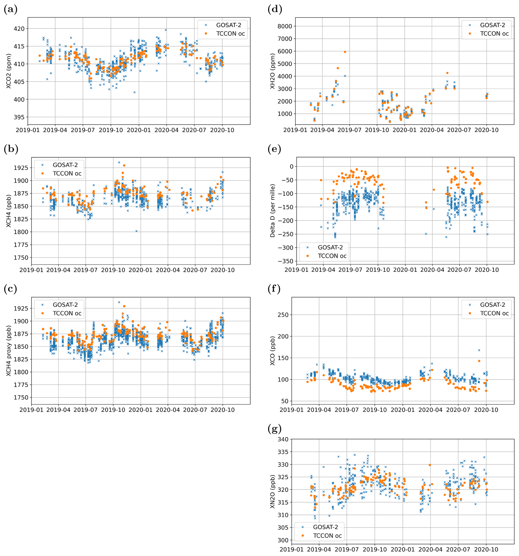
Figure 16Example time series of TCCON and GOSAT-2 FOCAL data at Lamont (station code oc). (a) XCO2; (b) XCH4 full-physics product; (c) XCH4 proxy product; (d) XH2O; (e) δD; (f) XCO; (g) XN2O.
4.3.2 XCH4 results versus TCCON
The FOCAL v3.0 full-physics XCH4 product for GOSAT has a station-to-station bias of 4.3 ppb (as given in pink at the bottom of Fig. 12), which is similar to the estimated 1σ TCCON uncertainty from Wunch et al. (2010) of 3.5 ppb and also compares well to the other data products. The value for the GOSAT FOCAL proxy product is 6.1 ppb, which is about 1–2 ppb higher than all other products but still in an acceptable range as it is better than the Copernicus systematic error threshold requirement of 10 ppb and close to the breakthrough requirement of better than 5 ppb (see Table 3 in Buchwitz et al., 2021). For GOSAT-2, FOCAL v3.0 has a station-to-station bias of 4.7 ppb for the full-physics XCH4 product and 6.2 ppb for the proxy.
The mean scatter of the GOSAT and GOSAT-2 FOCAL XCH4 product versus TCCON is around 12 ppb, which is slightly lower than for the other data products. The seasonal bias for all GOSAT and GOSAT-2 products relative to TCCON is around 3 ppb (Table 6). For both instruments, the temporal variations of the FOCAL full-physics and proxy XCH4 products agree well with the Lamont TCCON data (see Figs. 15b, c and 16b, c). In general, the FOCAL data are systematically lower by a few parts per billion (ppb), which is in line with the observed mean station bias of around −3 to −6 ppb; see Table 6.
4.3.3 XH2O results versus TCCON
Since water vapour is highly variable, the comparison results depend strongly on the involved TCCON stations. Because of the less strict filter criteria for XH2O, there are typically more data (and collocations) at higher latitudes than for the other full-physics products. We get a similar mean scatter of about 300 ppm for GOSAT and GOSAT-2 FOCAL XH2O. The station-to-station bias is 116 ppm for GOSAT and 152 ppm for GOSAT-2, which is even lower than the TCCON uncertainty of 200 ppm estimated by Wunch et al. (2010). The seasonal bias for GOSAT-2 is 110 ppm; for GOSAT, it is even smaller (66 ppm); see Table 6 for all values. The derived station-to-station biases and mean scatter values are in line with results derived for the OCO-2 FOCAL product (206 and 293 ppm, respectively; see Reuter et al., 2017a). As also mentioned there, these high values can at least partly be attributed to the large natural variability of water vapour. This variability can also be seen in the time series at Lamont (Figs. 15d and 16d), which show the same seasonal variations of around 4000 ppm peak-to-peak for all data sets.
4.3.4 δD results versus TCCON
For δD, we get station-to-station biases of only 8.6 ‰ for both instruments; the mean scatter is about 32 ‰ for GOSAT and GOSAT-2. The seasonal bias for GOSAT is 6 ‰; the GOSAT-2 value is 13 ‰ (Table 6). The mean station bias is quite large (around −83 ‰ for GOSAT and GOSAT-2). This is slightly larger than corresponding values between about −20 ‰ and −70 ‰ derived from a GOSAT–TCCON comparison performed by Boesch et al. (2013) for data between April 2009 and June 2011. Note that there is no uncertainty estimate available for the TCCON δD data, so all numbers given here should be treated with caution. The Lamont time series (Figs. 15e and 16e) show a systematic offset between TCCON on GOSAT/GOSAT-2 in line with the mean station bias, but the seasonality is well reproduced, although the satellite data show a larger scatter.
4.3.5 XCO results versus TCCON
The TCCON comparison for XCO reveals a station-to-station bias of 4.3 ppb, a mean scatter of 7.7 ppb and a seasonal bias of 2.8 ppb (Table 6). In fact, the XCO bias and scatter vary strongly between TCCON stations (see Figs. 13 and 14), but the derived values agree quite well with the TCCON uncertainty for carbon monoxide of 2 ppb. The data at Lamont (Fig. 16f) show that the temporal variation of XCO is well captured by the FOCAL product, but there is a systematic offset in line with the mean station bias of about 15 ppb.
4.3.6 XN2O results versus TCCON
The FOCAL XN2O is a new data product that is so far not available from other groups performing retrievals on GOSAT-2 trace gas measurements. For XN2O, we get from the TCCON comparison a station-to-station bias of 1.6 ppb and a mean scatter of 4.0 ppb (Figs. 13 and 14). The seasonal bias is 1.6 ppb (Table 6). Since the corresponding 1σ TCCON uncertainty from Wunch et al. (2010) is 1.5 ppb, we consider this to be reasonable agreement. The values for XN2O are similar to the expected local XN2O variability of a few parts per billion (ppb) (see e.g. García et al., 2018), but it should be considered that the total column average has a larger variability than surface data due to variations in tropopause height. This can be seen from Fig. 16g: both TCCON and GOSAT-2 observe total column seasonal variations with peak-to-peak differences of about 8 ppb, which is in line with the time series results. There is no visible bias between TCCON and GOSAT-2, but the scatter of the GOSAT-2 data is larger.
An updated version (v3.0) of the FOCAL retrieval algorithm has been applied to GOSAT and GOSAT-2 measurements in the NIR and SWIR spectral regions. This results in a variety of trace gas products, all derived within one retrieval and at comparably low computational costs. For both GOSAT instruments, we determine full-physics products for carbon dioxide, methane, water vapour and δD as well as a proxy methane product. For GOSAT-2, also carbon monoxide and a nitrous oxide product are retrieved.
Overall, the yield of valid data is improved in GOSAT and GOSAT-2 FOCAL v3.0. The number of XCO2 full-physics data has increased by about 50 % for GOSAT and has even doubled for GOSAT-2. This is mainly due to relaxations in the filtering of data and improved post-processing. The proxy methane, carbon monoxide and XH2O products even have about 2 times more data than the full-physics products.
The new GOSAT and GOSAT-2 products have been compared with ground-based TCCON data to get a first quality assessment. All FOCAL data agree with TCCON within the uncertainties of both data sets.
The FOCAL XCO2 data product is not only in line with TCCON but also with many other satellite data sets. A near-real-time version of this data set will be used in the Copernicus Atmospheric Monitoring Service (CAMS) as input for meteorological models. The FOCAL XCH4 products fulfil the corresponding requirements of the EU/ESA Copernicus Earth observation programme. The FOCAL data sets also provide useful input for ensemble studies, which have shown that additional information about, for example, sources and sinks of greenhouse gases can be obtained by combination of different data sets (see, for example, Reuter et al., 2013, 2020).
The spatial distribution of all gases and their temporal variation look reasonable. We have presented the first results for a GOSAT-2 XN2O product. We observe an XN2O gradient between the tropics and higher latitudes of about 15 ppb which can be explained by variations in the tropopause height. A similar gradient has been seen in IASI data.
The accuracy of the GOSAT-2 FOCAL XN2O is in the order of a few parts per billion (ppb) for a single sounding. We expect this to be improved by averaging of data such that, for example, monthly or annually gridded products can provide interesting information about XN2O, especially since there are not many global satellite measurements available for this species.
The Simple cLImatological Model for atmospheric CO2 or CH4 (SLIMCO2 or SLIMCH4) has been developed to provide estimates of dry-air mole fraction profiles and column averages of atmospheric CO2 or CH4 with reasonable accuracy at minimum computational costs. A key application of SLIMCO2 or SLIMCH4 is to compute CO2 or CH4 a priori information for remote sensing algorithms, which is why it also provides estimates of the corresponding error covariance matrix which can be used, for example, by optimal estimation frameworks.
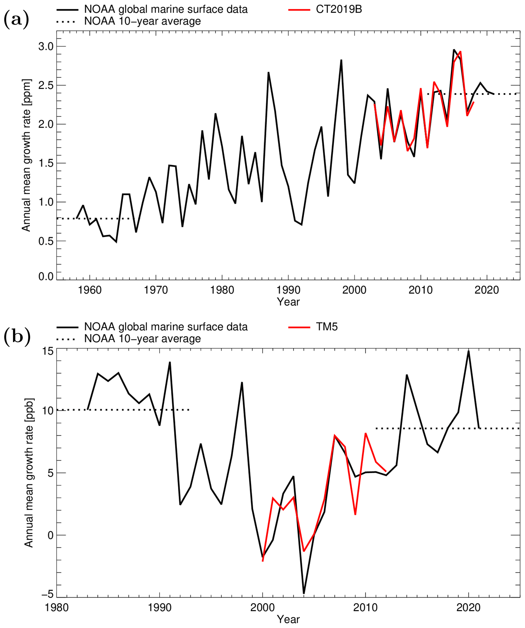
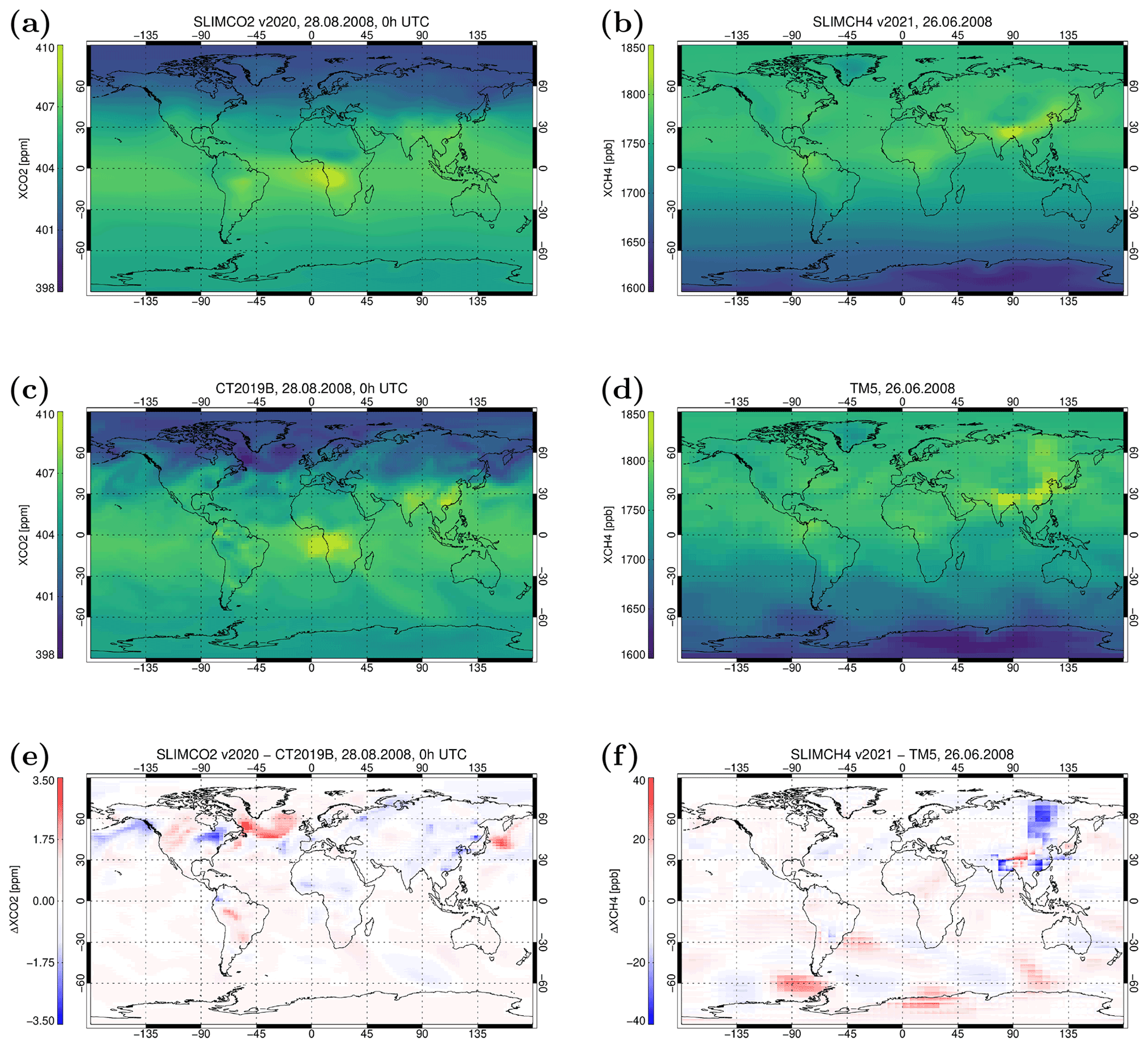
Figure A2Example maps of SLIMCO2 (a) and SLIMCH4 (b) data. Panels (c) and (d) show corresponding data from the underlying models (CT2019B, TM5). The differences between the SLIM results and these model data are shown in panels (e) and (f).
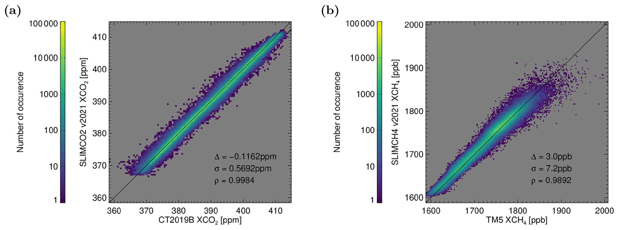
Figure A3Scatter plot of the data shown in Fig. A2. (a) SLIMCO2 data vs. CT2019B; (b) SLIMCH4 vs. TM5. Symbol σ corresponds to the standard deviation of the difference, δ corresponds to the average bias and ρ is the Pearson correlation coefficient.
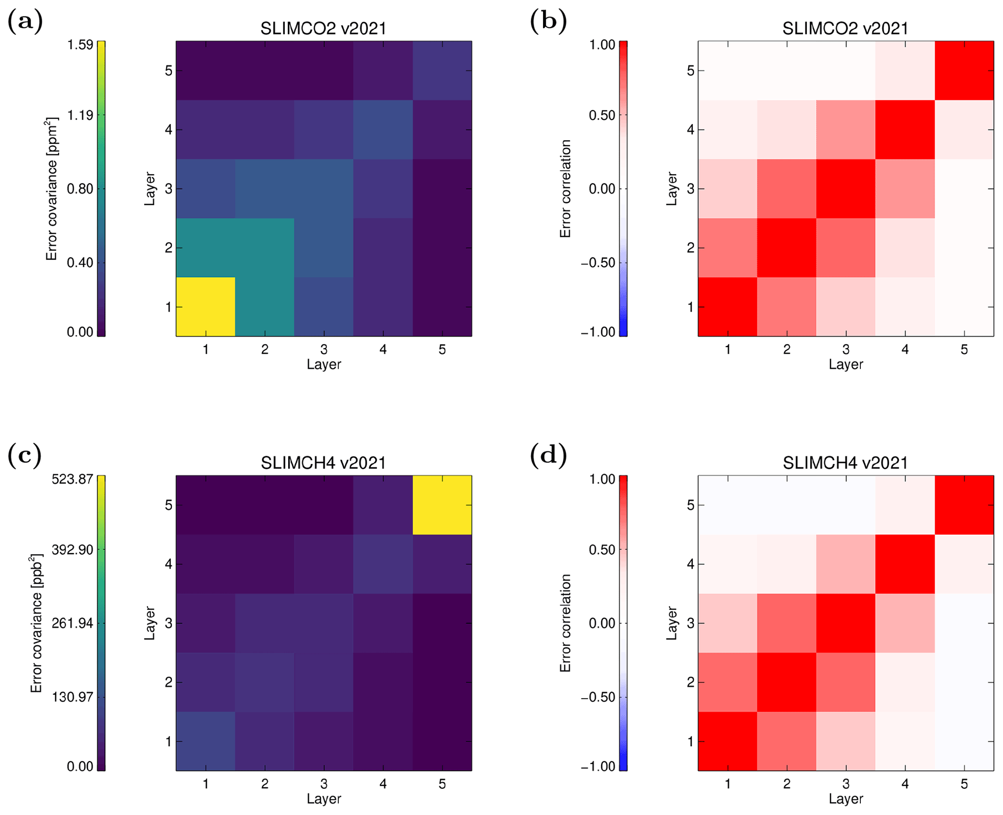
Figure A4Error covariance matrices for SLIMCO2 (a) and SLIMCH4 (c) and corresponding error correlation matrices (b, d).
The climatology database of SLIMCO2 v2021 has been derived from 16 years (2003–2018) of CO2 mole fraction data of NOAA's CarbonTracker model version CT2019B Jacobson et al. (2020). It has the same 3∘ × 2∘ spatial resolution as the used global CarbonTracker model fields. Temporally, it covers 1 year sampled in 36 time steps, corresponding to a grid resolution of about 10 d. The climatology database of SLIMCH4 v2021 has been derived from 13 years (2000–2012) of TM5–4DVAR CH4 mole fraction data (Bergamaschi et al., 2013) with a spatial resolution of 6∘ × 4∘. Temporally, it is sampled in 36 time steps, just as with the climatology database of SLIMCO2 v2021. Both databases feature a height grid with 20 layers. The height gridding is done in a way that each layer consists of the same number of dry-air particles so that the column average can simply be computed by averaging the mole-fraction profile. When reading the climatology database, SLIM allows for either nearest neighbour or trilinear interpolation in longitude, latitude and day of year. Additionally, SLIM is able to convert the height gridding to the one that is used, e.g. for the FOCAL OCO-2 XCO2 retrieval using five height layers for CO2.
First, we computed the global mean XGAS (XCO2 or XCH4) from the corresponding model for each 1 January (00:00 UTC) in the covered time period. In the next step, we went through all model time steps of the analysed period and subtracted the global mean XGAS, assuming linear growth within the years. Finally, we created the climatology databases by incrementally computing the average and standard deviation of the gases mole fraction of all growth-corrected model time steps falling into the 10 d temporal grid cells of the database. In this way, the created databases basically consist of growth-removed seasonal cycle anomalies.
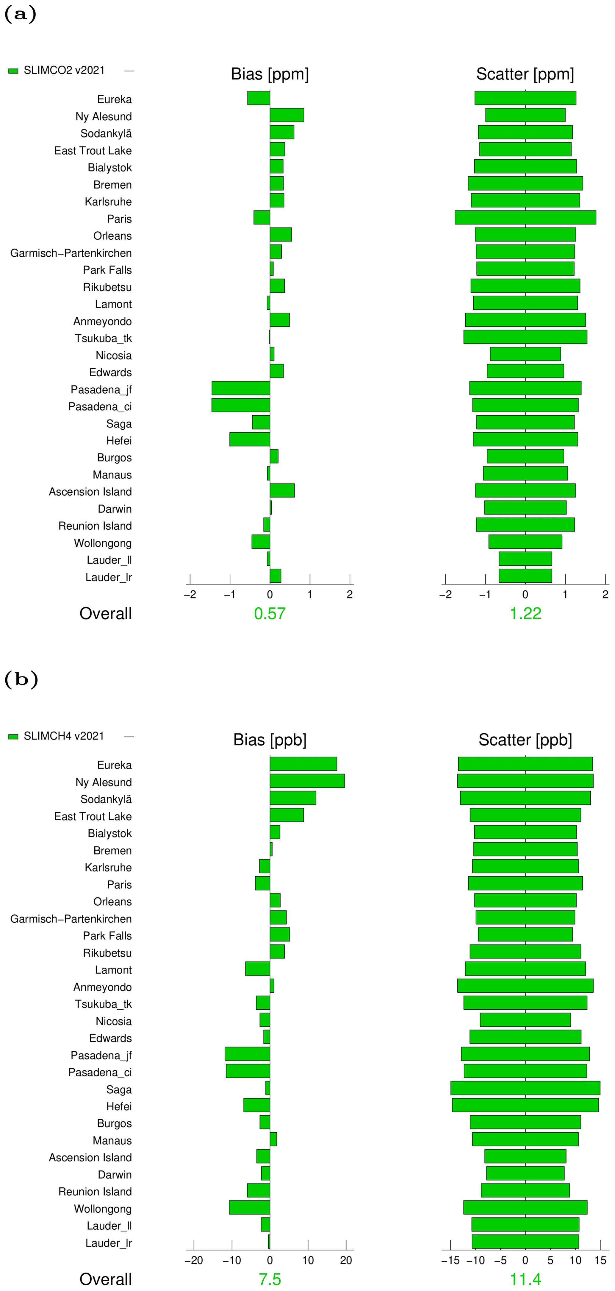
Figure A5Overview of TCCON validation results for SLIMCO2 (a) and SLIMCH4 (b). The mean station bias has been subtracted to better illustrate the local station differences.
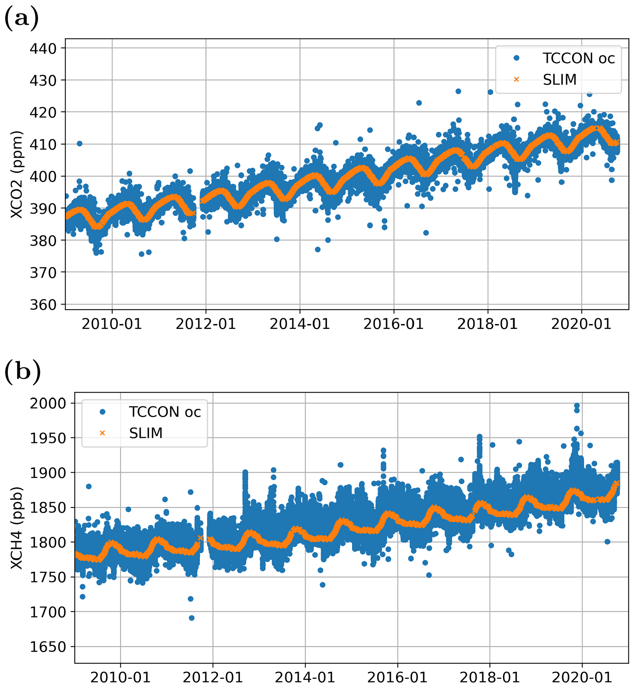
Figure A6Time series of XCO2 (a) and XCH4 (b) from TCCON and SLIM at Lamont (station code oc).
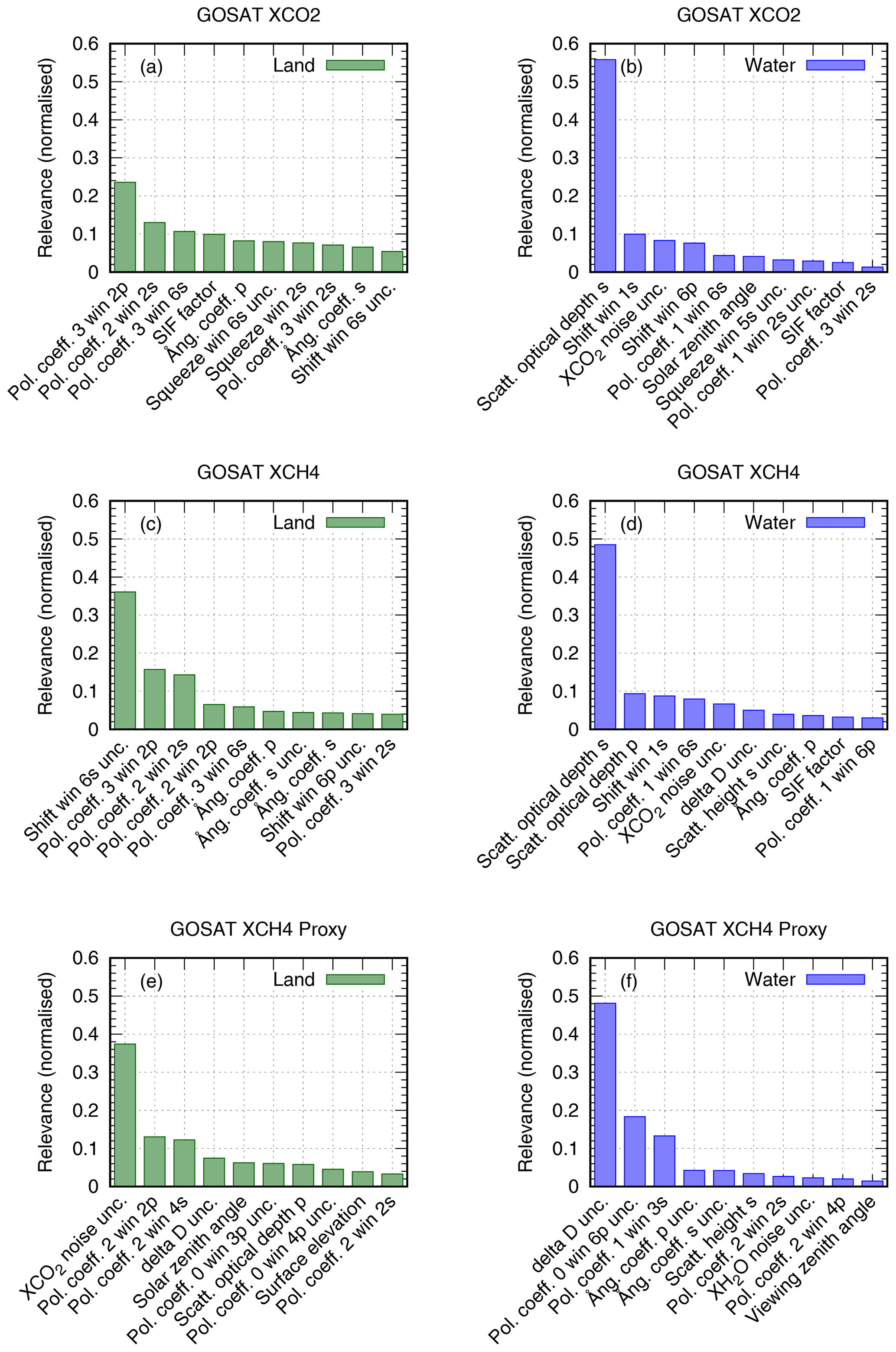
Figure A7Variables selected for the GOSAT random forest bias correction and their relevance. (a, b) XCO2; (c, d) XCH4; (e, f) XCH4 Proxy. Left and right columns are for land and water surfaces, respectively.
In addition to the created 4D data fields, the database contains a table of annual growth rates obtained from NOAA (https://gml.noaa.gov/ccgg/trends/gr.html, last access: 3 July 2021). Currently, the implemented table covers the time periods 1959–2020 for CO2 and 1984–2020 for CH4, but it can be extended if needed to improve the quality of SLIM estimates in years before or after these periods. Fig. A1 shows the NOAA annual mean growth rates for CO2 and CH4 computed from global marine surface data as stored in the database. As visible in the figure, the NOAA growth rate agrees well with the growth computed from the model data as described above.
In the following, we describe how SLIM uses its database to estimate the CO2 or CH4 atmospheric dry-air mole fraction for a given longitude, latitude and time. The database has been generated as follows. First, SLIM computes an estimate of the global average mole fraction by linear interpolation in the accumulated growth rates database. Note that extrapolation to dates outside of the spanned period is done by assuming a 10-year average growth rate (dashed lines in Fig. A1). This global average is added to the mole fraction anomaly interpolated from the corresponding 4D database field for the given longitude, latitude and day of year.
Figure A2 shows examples of a global XCO2 and XCH4 map as read from the models (panels c and d) and in panels (a) and (b) for the corresponding maps of SLIM XGAS values. Since the SLIM layers are defined such that they all contain the same number of dry-air particles, the SLIM XGAS values can be computed as mean of all layer values. As one can also see in the difference maps (panels e and f), the large-scale patterns such as north–south gradient are well reproduced, and differences are mainly due the specific synoptic situation in the model field, which usually changes from year to year and which, therefore, cannot be reproduced by a simple climatology. For the example of CO2, the largest natural surface fluxes occur during the northern hemispheric growing season. Therefore, the largest deviations between CT2019B and SLIMCO2 occur in the Northern Hemisphere in Fig. A2e.
By comparing 1 million randomly selected profiles in the period 2003–2018, we computed that the SLIMCO2 XCO2 is on average 0.1 ppm lower than the corresponding CarbonTracker values, with a standard deviation of 0.57 ppm and a correlation coefficient of 0.998 (see Fig. A3a). The corresponding experiment for SLIMCH4 results in a mean difference of 3 ppb, a standard deviation of the difference of 7.2 ppb and a correlation coefficient of 0.989 (see Fig. A3b).
The error covariance matrix for the 5-layered SLIMCO2 profiles shown in Fig. A4a shows the largest uncertainties in the lowermost layer (approx. 1000–800 hPa), which is influenced strongest by the surface fluxes and the smallest uncertainties in the uppermost layer (approx. 200–0 hPa) including the stratosphere. The largest error correlations exist between layers 1–4, whilst the uncertainties of layer 5 are relatively independent (Fig. A4b). For CH4, the correlation structure is similar (Fig. A4d), but the largest uncertainties are observed in the stratosphere (Fig. A4c).
Also the comparison of SLIM with corresponding TCCON XGAS measurements show good overall agreement (Figs. A5 and A6). Analysed in the same way as done in the validation study by Reuter et al. (2020), we find CO2 biases with a station-to-station standard deviation of 0.57 ppm and an average scatter of 1.14 ppm with respect to TCCON (Fig. A5a). For CH4, we find biases with a station-to-station standard deviation of 7.5 ppb and an average scatter of 10.6 ppb (Fig. A5b). Especially for XCO2, these values are similar to values found for comparisons of satellite retrieval data products with TCCON (e.g. Reuter et al., 2020).
Table A1XCO2 filter variables and limits for GOSAT. “–” means that no limit is applied. Except for the solar zenith angle limits, the variables are ordered by their relevance, i.e. by the number of data filtered out.
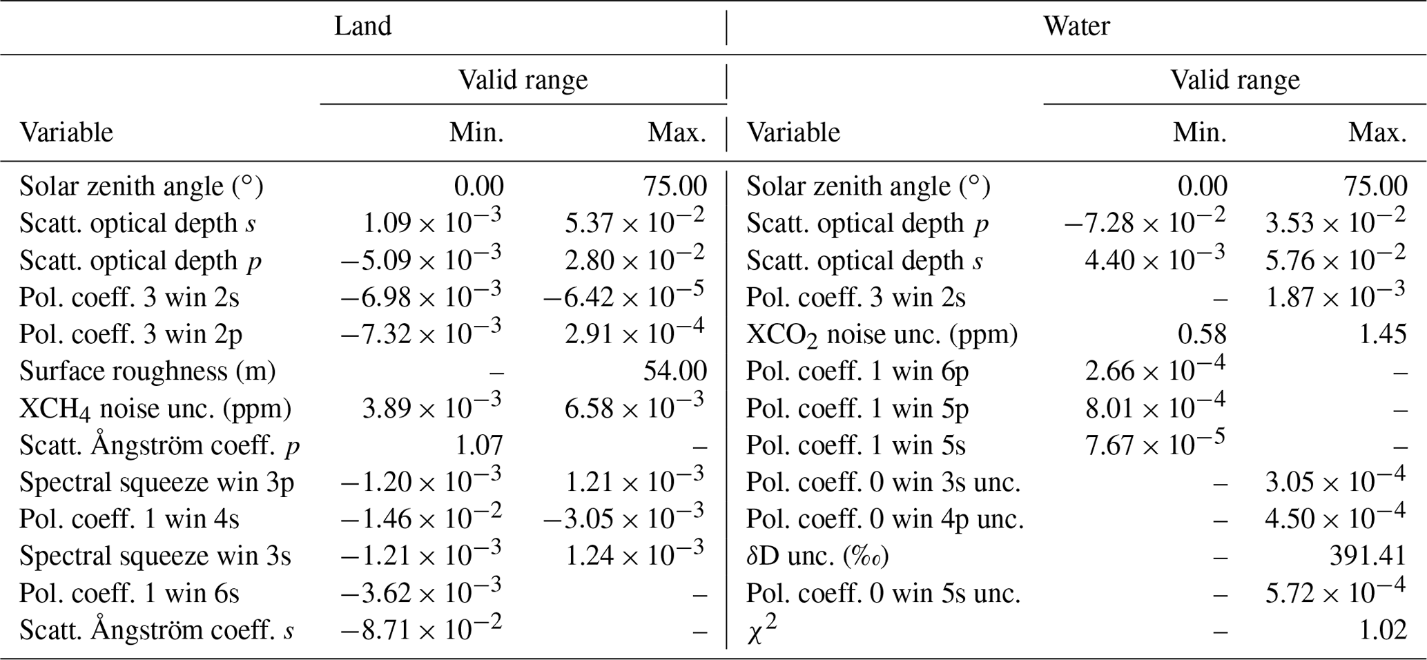
Table A2XCH4 filter variables and limits for GOSAT. “–” means that no limit is applied. Except for the solar zenith angle limits, the variables are ordered by their relevance, i.e. by the number of data filtered out.
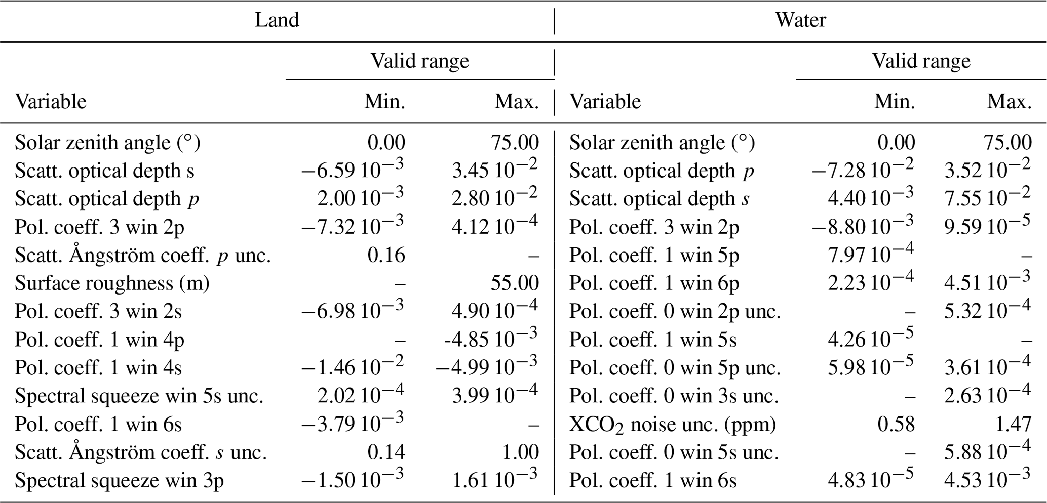
Table A3XCH4 Proxy filter variables and limits for GOSAT. “–” means that no limit is applied. Except for the solar zenith angle limits, the variables are ordered by their relevance, i.e. by the number of data filtered out.
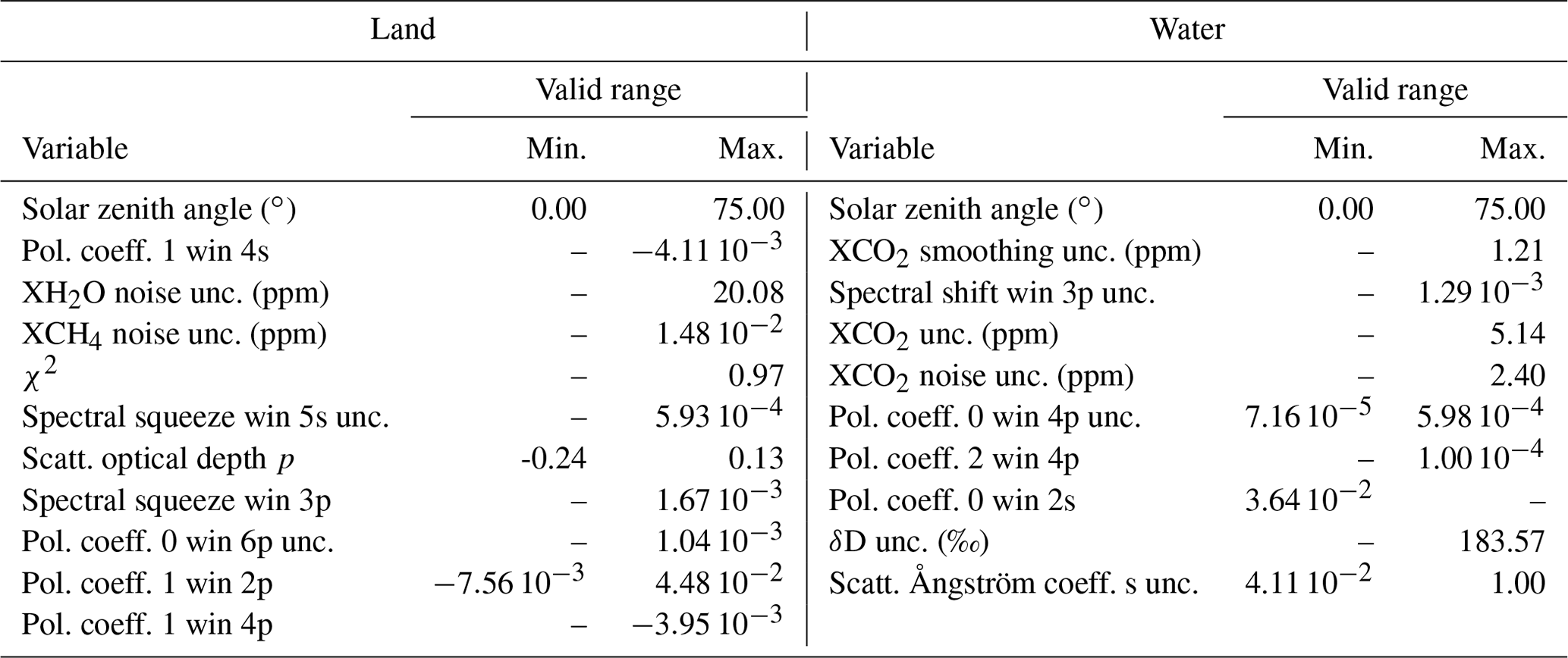
Table A4XH2O filter variables and limits for GOSAT. “–” means that no limit is applied. The variables are ordered by their relevance, i.e. by the number of data filtered out.
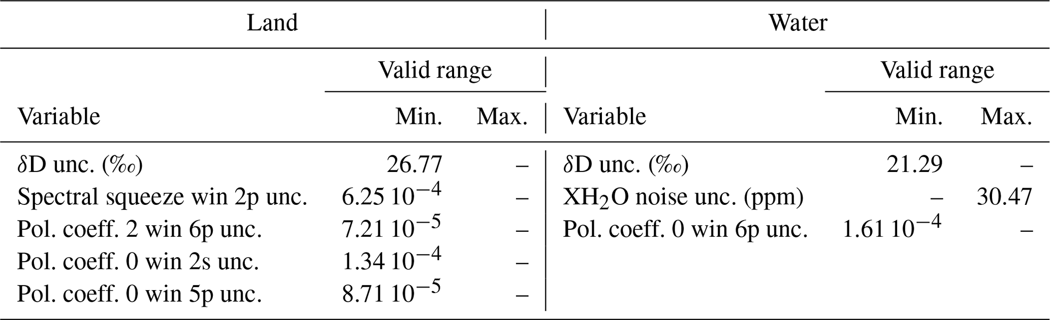
Table A5δD filter variables and limits for GOSAT. “–” means that no limit is applied. Except for the solar zenith angle limits, the variables are ordered by their relevance, i.e. by the number of data filtered out.
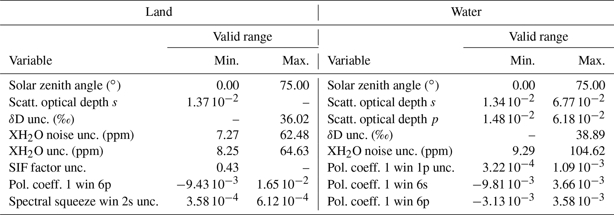
Table A6XCO2 filter variables and limits for GOSAT-2. “–” means that no limit is applied. Except for the solar zenith angle limits, the variables are ordered by their relevance, i.e. by the number of data filtered out.
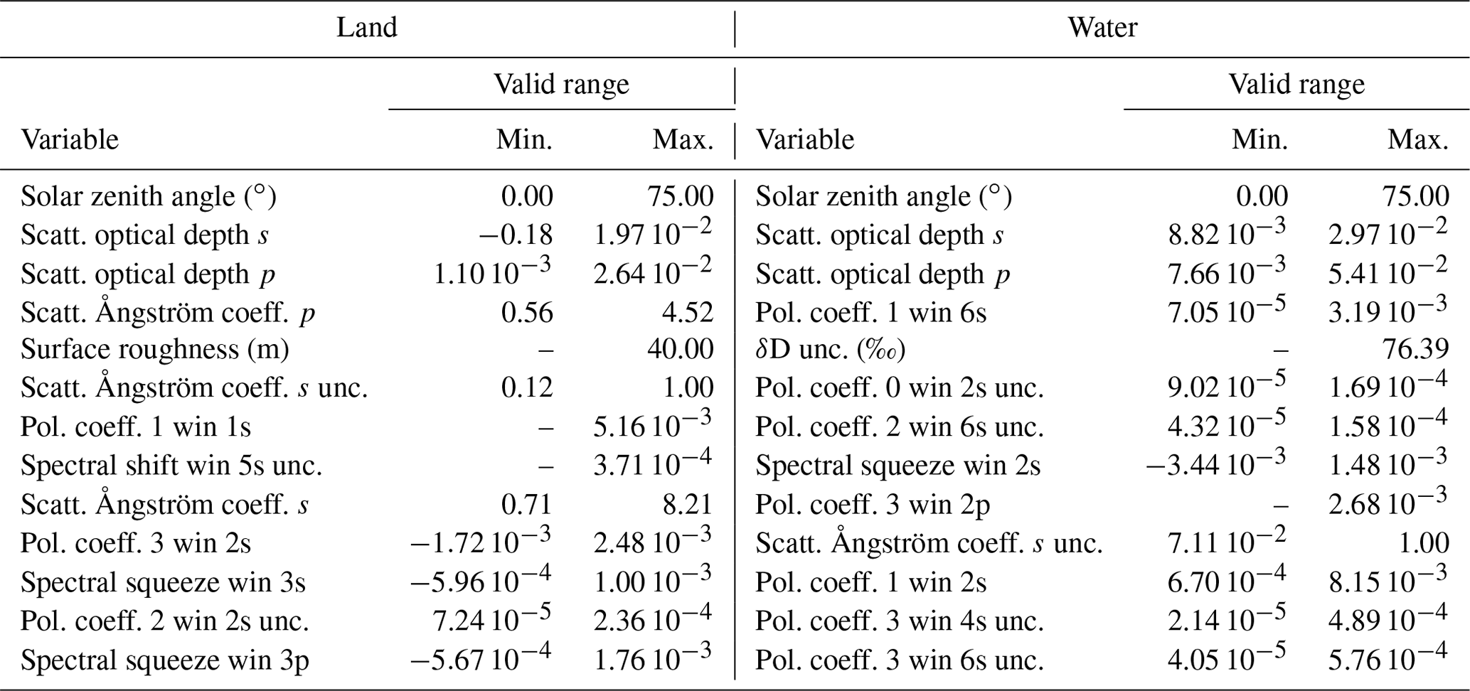
Table A7XCH4 filter variables and limits for GOSAT-2. “–” means that no limit is applied. Except for the solar zenith angle limits, the variables are ordered by their relevance, i.e. by the number of data filtered out.
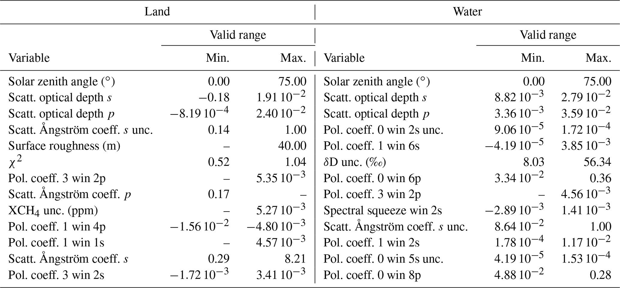
Table A8XCH4 Proxy filter variables and limits for GOSAT-2. “–” means that no limit is applied. Except for the solar zenith angle limits, the variables are ordered by their relevance, i.e. by the number of data filtered out.
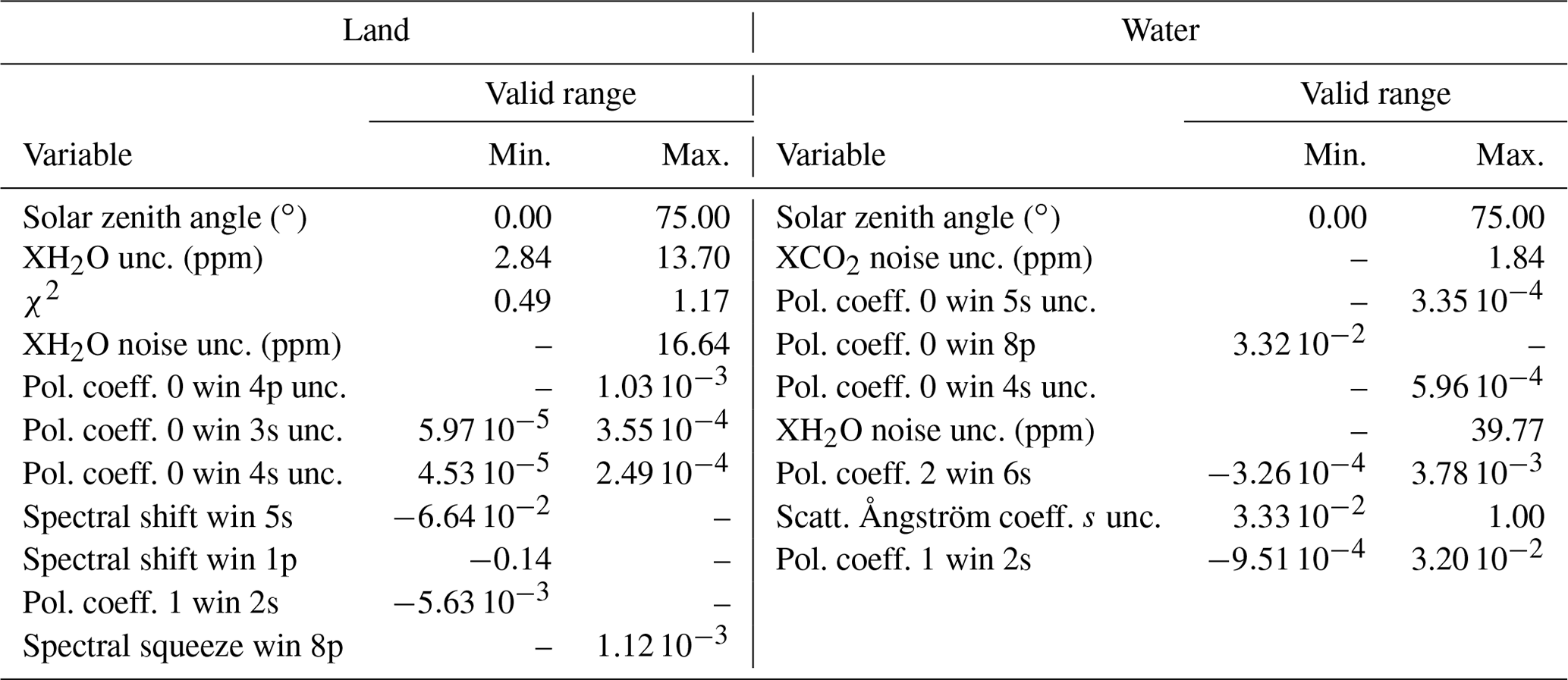
Table A9XH2O filter variables and limits for GOSAT-2. “–” means that no limit is applied. The variables are ordered by their relevance, i.e. by the number of data filtered out.

Table A10δD filter variables and limits for GOSAT-2. “–” means that no limit is applied. Except for the solar zenith angle limits, the variables are ordered by their relevance, i.e. by the number of data filtered out.
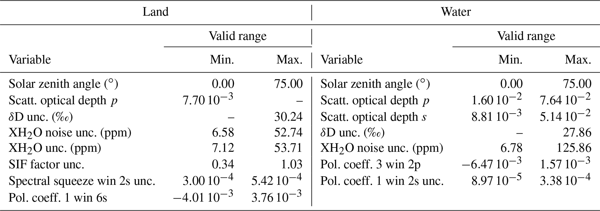
Table A11XCO filter variables and limits for GOSAT-2. “–” means that no limit is applied. Except for the solar zenith angle limits, the variables are ordered by their relevance, i.e. by the number of data filtered out.
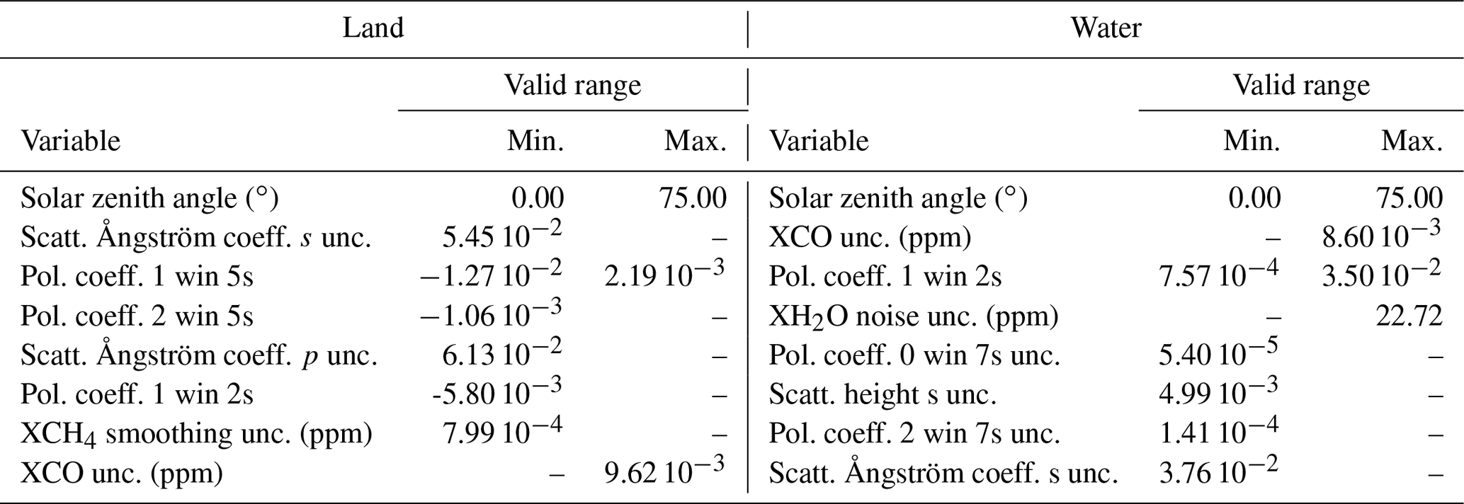
Table A12XN2O filter variables and limits for GOSAT-2. “–” means that no limit is applied. Except for the solar zenith angle limits, the variables are ordered by their relevance, i.e. by the number of data filtered out.
The GOSAT and GOSAT-2 FOCAL v3.0 data sets are available on request from the authors.
SN adapted the FOCAL method to GOSAT and GOSAT-2, generated the updated FOCAL data products and performed the validation. MR developed the FOCAL method and provided the XCO2 and XCH4 reference databases and the TCCON validation tools. JPB provided the used Python implementation for the SLIM XCO2 and methane climatology. MH provided the original Python implementation of FOCAL (OCO-2 version). ADN and RJP provided the UoL data, and YY provided the NIES GOSAT data products. The following co-authors provided TCCON data: MB, NMD, DGF, DWTG, FH, RK, CL, YO, IM, JN, HO, CP, DFP, MR, CR, CR, MKS, KS, KS, RS, YT, VAV, MV and TW. All authors provided support in writing the paper.
At least one of the (co-)authors is a member of the editorial board of Atmospheric Measurement Techniques.
Publisher’s note: Copernicus Publications remains neutral with regard to jurisdictional claims in published maps and institutional affiliations.
GOSAT and GOSAT-2 spectral data have been provided by JAXA and NIES. CarbonTracker CT2019B and CT-NRT.v2020-1 results were provided by NOAA ESRL, Boulder, Colorado, USA, from the website at http://carbontracker.noaa.gov (last access: 2 June 2022). ABSCO cross sections for CO2 were provided by NASA and the ACOS/OCO-2 team. GMTED2010 topography data were provided by the U.S. Geological Survey (USGS) and the National Geospatial-Intelligence Agency (NGA). We thank the European Centre for Medium-Range Weather Forecasts (ECMWF) for providing us with analysed meteorological fields (ERA5 data).
The GOSAT ACOS v9 Level 2 XCO2 product from the NASA/OCO-2 team has been obtained from https://oco2.gesdisc.eosdis.nasa.gov/data/GOSAT_TANSO_Level2/ACOS_L2_Lite_FP.9r/, https://doi.org/10.5067/VWSABTO7ZII4 (last access: 16 October 2020). The UoL and SRON GOSAT data products have been obtained from the Copernicus Climate Data Store (https://cds.climate.copernicus.eu/, last assess: 15 October 2020). GOSAT Level 2 data from NIES have been provided by the GOSAT Data Archive Service (GDAS; https://data2.gosat.nies.go.jp/, last access: 17 January 2022).
RJP is funded via the UK National Centre for Earth Observation (NE/N018079/1). This research used the ALICE High Performance Computing Facility at the University of Leicester for the UoL GOSAT retrievals.
The Paris TCCON site has received funding from Sorbonne Université, the French research centre CNRS, the French space agency CNES and Région Île-de-France. The Réunion station is operated by the Royal Belgian Institute for Space Aeronomy with financial support since 2014 by the EU project ICOS-Inwire and the ministerial decree for ICOS (FR/35/IC1 to FR/35/IC6) as well as local activities supported by LACy/UMR8105 – Université de La Réunion. The TCCON stations at Rikubetsu, Tsukuba and Burgos are supported in part by the GOSAT series project. Local support for Burgos is provided by the Energy Development Corporation (EDC, Philippines). The Eureka measurements were made at the Polar Environment Atmospheric Research Laboratory (PEARL) by the Canadian Network for the Detection of Atmospheric Change (CANDAC), primarily supported by the Natural Sciences and Engineering Research Council of Canada, Environment and Climate Change Canada, and the Canadian Space Agency. The Anmyeondo TCCON station is funded by the Korea Meteorological Administration research and development programme “Development of Monitoring and Analysis Techniques for Atmospheric Composition in Korea” under grant KMA2018-00522. The TCCON Nicosia site has received support from the European Unions’ Horizon 2020 research and innovation programme under grant agreement no. 856612 (EMME-CARE), the Cyprus Government, and by the University of Bremen. NMD is supported by an Australian Research Council (ARC) Future Fellowship (FT180100327). The Darwin and Wollongong TCCON sites have been supported by a series of ARC grants, including DP160100598, DP140100552, DP110103118, DP0879468 and LE0668470, and NASA grants NAG5-12247 and NNG05-GD07G.
Large parts of the calculations reported here were performed on high-performance computing (HPC) facilities of the IUP, University of Bremen, funded under DFG/FUGG grant INST 144/379-1 and INST 144/493-1. The work was supported by the Copernicus Atmosphere Monitoring Service (CAMS) via project CAMS2-52b.
This work has received funding from JAXA (GOSAT and GOSAT-2 support, contracts 19RT000692 and JX-PSPC-527269), EUMETSAT (FOCAL-CO2M study, contract EUM/CO/19/4600002372/RL), ESA (GHG-CCI+ project, contract 4000126450/19/I-NB), and the state and the University of Bremen.
This research has been supported by the Japan Aerospace Exploration Agency (grant nos. 19RT000692 and JX-PSPC-527269), the European Organization for the Exploitation of Meteorological Satellites (grant no. EUM/CO/19/4600002372/RL) and the European Space Agency (grant no. 4000126450/19/I-NB).
The article processing charges for this open-access publication were covered by the University of Bremen.
This paper was edited by Alexander Kokhanovsky and reviewed by T. E. Taylor and three anonymous referees.
Barret, B., Gouzenes, Y., Le Flochmoen, E., and Ferrant, S.: Retrieval of Metop-A/IASI N2O Profiles and Validation with NDACC FTIR Data, Atmosphere, 12, 219, https://doi.org/10.3390/atmos12020219, 2021. a, b, c, d
Bergamaschi, P., Houweling, S., Segers, A., Krol, M., Frankenberg, C., Scheepmaker, R. A., Dlugokencky, E., Wofsy, S. C., Kort, E. A., Sweeney, C., Schuck, T., Brenninkmeijer, C., Chen, H., Beck, V., and Gerbig, C.: Atmospheric CH4 in the first decade of the 21st century: Inverse modeling analysis using SCIAMACHY satellite retrievals and NOAA surface measurements, J. Geophys. Res.-Atmos., 118, 7350–7369, https://doi.org/10.1002/jgrd.50480, 2013. a
Blumenstock, T., Hase, F., Schneider, M., García, O. E., and Sepúlveda, E.: TCCON data from Izana (ES), Release GGG2014.R1, Caltech Library [data set], https://doi.org/10.14291/TCCON.GGG2014.IZANA01.R1, 2017. a
Boesch, H., Deutscher, N. M., Warneke, T., Byckling, K., Cogan, A. J., Griffith, D. W. T., Notholt, J., Parker, R. J., and Wang, Z.: HDO/H2O ratio retrievals from GOSAT, Atmos. Meas. Tech., 6, 599–612, https://doi.org/10.5194/amt-6-599-2013, 2013. a, b
Borger, C., Beirle, S., and Wagner, T.: Analysis of global trends of total column water vapour from multiple years of OMI observations, Atmos. Chem. Phys. Discuss. [preprint], https://doi.org/10.5194/acp-2022-149, in review, 2022. a
Buchwitz, M., Reuter, M., Schneising-Weigel, O., Aben, I., Wu, L., Hasekamp, O. P., Boesch, H., Noia, A. D., Crevoisier, C., and Armante, R.: Target Requirements and Gap Analysis Document: Greenhouse Gases (CO2 & CH4), Tech. Rep. v3.1 19-02-2021, Copernicus Climate Change Service C3S, http://wdc.dlr.de/C3S_312b_Lot2/Documentation/GHG/TRD-GAD/C3S_D312b_Lot2.1.0-2020(GHG)_TRD-GAD_v3.1.pdf (last access: 31 January 2022), 2021. a
Butz, A., Guerlet, S., Hasekamp, O., Schepers, D., Galli, A., Aben, I., Frankenberg, C., Hartmann, J.-M., Tran, H., Kuze, A., Keppel-Aleks, G., Toon, G., Wunch, D., Wennberg, P., Deutscher, N., Griffith, D., Macatangay, R., Messerschmidt, J., Notholt, J., and Warneke, T.: Toward accurate CO2 and CH4 observations from GOSAT, Geophys. Res. Lett., 38, L14812, https://doi.org/10.1029/2011GL047888, 2011. a, b
Cogan, A. J., Boesch, H., Parker, R. J., Feng, L., Palmer, P. I., Blavier, J.-F. L., Deutscher, N. M., Macatangay, R., Notholt, J., Roehl, C., Warneke, T., and Wunch, D.: Atmospheric carbon dioxide retrieved from the Greenhouse gases Observing SATellite (GOSAT): Comparison with ground-based TCCON observations and GEOS-Chem model calculations, J. Geophys. Res.-Atmos., 117, D21301, https://doi.org/10.1029/2012JD018087, 2012. a, b
Crisp, D., Pollock, H. R., Rosenberg, R., Chapsky, L., Lee, R. A. M., Oyafuso, F. A., Frankenberg, C., O'Dell, C. W., Bruegge, C. J., Doran, G. B., Eldering, A., Fisher, B. M., Fu, D., Gunson, M. R., Mandrake, L., Osterman, G. B., Schwandner, F. M., Sun, K., Taylor, T. E., Wennberg, P. O., and Wunch, D.: The on-orbit performance of the Orbiting Carbon Observatory-2 (OCO-2) instrument and its radiometrically calibrated products, Atmos. Meas. Tech., 10, 59–81, https://doi.org/10.5194/amt-10-59-2017, 2017. a
Danielson, J. and Gesch, D.: Global multi-resolution terrain elevation data 2010 (GMTED2010): Open-File Report 2011–1073, Tech. rep., U.S. Geol. Surv., 26 p., https://doi.org/10.3133/ofr20111073, 2011. a
De Mazière, M., Sha, M. K., Desmet, F., Hermans, C., Scolas, F., Kumps, N., Metzger, J.-M., Duflot, V., and Cammas, J.-P.: TCCON data from Réunion Island (RE), Release GGG2014.R1, Caltech Library [data set], https://doi.org/10.14291/TCCON.GGG2014.REUNION01.R1, 2017. a
Deutscher, N. M., Notholt, J., Messerschmidt, J., Weinzierl, C., Warneke, T., Petri, C., and Grupe, P.: TCCON data from Bialystok (PL), Release GGG2014.R2, Caltech Library [data set] https://doi.org/10.14291/TCCON.GGG2014.BIALYSTOK01.R2, 2019. a
Dubey, M., Lindenmaier, R., Henderson, B., Green, D., Allen, N., Roehl, C., Blavier, J.-F., Butterfield, Z., Love, S., Hamelmann, J., and Wunch, D.: TCCON data from Four Corners (US), Release GGG2014R0, TCCON data archive, hosted by CaltechDATA, Caltech Library [data set] https://doi.org/10.14291/tccon.ggg2014.fourcorners01.R0/1149272, 2014. a
Dupuy, E., Morino, I., Deutscher, N. M., Yoshida, Y., Uchino, O., Connor, B. J., De Mazière, M., Griffith, D. W. T., Hase, F., Heikkinen, P., Hillyard, P. W., Iraci, L. T., Kawakami, S., Kivi, R., Matsunaga, T., Notholt, J., Petri, C., Podolske, J. R., Pollard, D. F., Rettinger, M., Roehl, C. M., Sherlock, V., Sussmann, R., Toon, G. C., Velazco, V. A., Warneke, T., Wennberg, P. O., Wunch, D., and Yokota, T.: Comparison of XH2O Retrieved from GOSAT Short-Wavelength Infrared Spectra with Observations from the TCCON Network, Remote Sens., 8, 414, https://doi.org/10.3390/rs8050414, 2016. a
Eldering, A., O'Dell, C. W., Wennberg, P. O., Crisp, D., Gunson, M. R., Viatte, C., Avis, C., Braverman, A., Castano, R., Chang, A., Chapsky, L., Cheng, C., Connor, B., Dang, L., Doran, G., Fisher, B., Frankenberg, C., Fu, D., Granat, R., Hobbs, J., Lee, R. A. M., Mandrake, L., McDuffie, J., Miller, C. E., Myers, V., Natraj, V., O'Brien, D., Osterman, G. B., Oyafuso, F., Payne, V. H., Pollock, H. R., Polonsky, I., Roehl, C. M., Rosenberg, R., Schwandner, F., Smyth, M., Tang, V., Taylor, T. E., To, C., Wunch, D., and Yoshimizu, J.: The Orbiting Carbon Observatory-2: first 18 months of science data products, Atmos. Meas. Tech., 10, 549–563, https://doi.org/10.5194/amt-10-549-2017, 2017. a
Feist, D. G., Arnold, S. G., John, N., and Geibel, M. C.: TCCON data from Ascension Island (SH), Release GGG2014R0, TCCON data archive, CaltechDATA [data set], https://doi.org/10.14291/tccon.ggg2014.ascension01.R0/1149285, 2014. a
Frankenberg, C., Wunch, D., Toon, G., Risi, C., Scheepmaker, R., Lee, J.-E., Wennberg, P., and Worden, J.: Water vapor isotopologue retrievals from high-resolution GOSAT shortwave infrared spectra, Atmos. Meas. Tech., 6, 263–274, https://doi.org/10.5194/amt-6-263-2013, 2013. a, b
García, O. E., Schneider, M., Ertl, B., Sepúlveda, E., Borger, C., Diekmann, C., Wiegele, A., Hase, F., Barthlott, S., Blumenstock, T., Raffalski, U., Gómez-Peláez, A., Steinbacher, M., Ries, L., and de Frutos, A. M.: The MUSICA IASI CH4 and N2O products and their comparison to HIPPO, GAW and NDACC FTIR references, Atmos. Meas. Tech., 11, 4171–4215, https://doi.org/10.5194/amt-11-4171-2018, 2018. a
Goo, T.-Y., Oh, Y.-S., and Velazco, V. A.: TCCON data from Anmeyondo (KR), Release GGG2014R0, TCCON data archive, CaltechDATA [data set], https://doi.org/10.14291/tccon.ggg2014.anmeyondo01.R0/1149284, 2014. a
Gordon, I., Rothman, L., Hill, C., Kochanov, R., Tan, Y., Bernath, P., Birk, M., Boudon, V., Campargue, A., Chance, K., Drouin, B., Flaud, J.-M., Gamache, R., Hodges, J., Jacquemart, D., Perevalov, V., Perrin, A., Shine, K., Smith, M.-A., Tennyson, J., Toon, G., Tran, H., Tyuterev, V., Barbe, A., Császár, A., Devi, V., Furtenbacher, T., Harrison, J., Hartmann, J.-M., Jolly, A., Johnson, T., Karman, T., Kleiner, I., Kyuberis, A., Loos, J., Lyulin, O., Massie, S., Mikhailenko, S., Moazzen-Ahmadi, N., Müller, H., Naumenko, O., Nikitin, A., Polyansky, O., Rey, M., Rotger, M., Sharpe, S., Sung, K., Starikova, E., Tashkun, S., Auwera, J. V., Wagner, G., Wilzewski, J., Wcisło, P., Yu, S., and Zak, E.: The HITRAN2016 molecular spectroscopic database, J. Quant. Spectr. Rad. Transf., 203, 3–69, https://doi.org/10.1016/j.jqsrt.2017.06.038, hITRAN2016 Special Issue, 2017. a
Gorshelev, V., Serdyuchenko, A., Weber, M., Chehade, W., and Burrows, J. P.: High spectral resolution ozone absorption cross-sections – Part 1: Measurements, data analysis and comparison with previous measurements around 293 K, Atmos. Meas. Tech., 7, 609–624, https://doi.org/10.5194/amt-7-609-2014, 2014. a
Griffith, D. W., Deutscher, N. M., Velazco, V. A., Wennberg, P. O., Yavin, Y., Aleks, G. K., Washenfelder, R. A., Toon, G. C., Blavier, J.-F., Murphy, C., Jones, N., Kettlewell, G., Connor, B. J., Macatangay, R., Roehl, C., Ryczek, M., Glowacki, J., Culgan, T., and Bryant, G.: TCCON data from Darwin (AU), Release GGG2014R0, TCCON data archive, CaltechDATA [data set], https://doi.org/10.14291/tccon.ggg2014.darwin01.R0/1149290, 2014a. a
Griffith, D. W., Velazco, V. A., Deutscher, N. M., Murphy, C., Jones, N., Wilson, S., Macatangay, R., Kettlewell, G., Buchholz, R. R., and Riggenbach, M.: TCCON data from Wollongong (AU), Release GGG2014R0, TCCON data archive, CaltechDATA [data set], https://doi.org/10.14291/tccon.ggg2014.wollongong01.R0/1149291, 2014b. a
Hase, F., Blumenstock, T., Dohe, S., Gross, J., and Kiel, M.: TCCON data from Karlsruhe (DE), Release GGG2014R1, TCCON data archive, CaltechDATA [data set], https://doi.org/10.14291/tccon.ggg2014.karlsruhe01.R1/1182416, 2014. a
Hersbach, H., Bell, B., Berrisford, P., Hirahara, S., Horányi, A., Muñoz Sabater, J., Nicolas, J., Peubey, C., Radu, R., Schepers, D., Simmons, A., Soci, C., Abdalla, S., Abellan, X., Balsamo, G., Bechtold, P., Biavati, G., Bidlot, J., Bonavita, M., De Chiara, G., Dahlgren, P., Dee, D., Diamantakis, M., Dragani, R., Flemming, J., Forbes, R., Fuentes, M., Geer, A., Haimberger, L., Healy, S., Hogan, R. J., Hólm, E., Janisková, M., Keeley, S., Laloyaux, P., Lopez, P., Lupu, C., Radnoti, G., de Rosnay, P., Rozum, I., Vamborg, F., Villaume, S., and Thépaut, J.-N.: The ERA5 global reanalysis, Q. J. Roy. Meteorol. Soc., 146, 1999–2049, https://doi.org/10.1002/qj.3803, 2020. a
Heymann, J., Reuter, M., Hilker, M., Buchwitz, M., Schneising, O., Bovensmann, H., Burrows, J. P., Kuze, A., Suto, H., Deutscher, N. M., Dubey, M. K., Griffith, D. W. T., Hase, F., Kawakami, S., Kivi, R., Morino, I., Petri, C., Roehl, C., Schneider, M., Sherlock, V., Sussmann, R., Velazco, V. A., Warneke, T., and Wunch, D.: Consistent satellite XCO2 retrievals from SCIAMACHY and GOSAT using the BESD algorithm, Atmos. Meas. Tech., 8, 2961–2980, https://doi.org/10.5194/amt-8-2961-2015, 2015. a
Iraci, L. T., Podolske, J., Hillyard, P. W., Roehl, C., Wennberg, P. O., Blavier, J.-F., Allen, N., Wunch, D., Osterman, G. B., and Albertson, R.: TCCON data from Edwards (US), Release GGG2014R1, TCCON data archive, CaltechDATA [data set], https://doi.org/10.14291/tccon.ggg2014.edwards01.R1/1255068, 2016a. a
Iraci, L. T., Podolske, J., Hillyard, P. W., Roehl, C., Wennberg, P. O., Blavier, J.-F., Landeros, J., Allen, N., Wunch, D., Zavaleta, J., Quigley, E., Osterman, G. B., Barrow, E., and Barney, J.: TCCON data from Indianapolis (US), Release GGG2014R1, TCCON data archive, CaltechDATA [data set], https://doi.org/10.14291/tccon.ggg2014.indianapolis01.R1/1330094, 2016b. a
Jacobson, A. R., Schuldt, K. N., Miller, J. B., Oda, T., Tans, P., Arlyn Andrews, Mund, J., Ott, L., Collatz, G. J., Aalto, T., Afshar, S., Aikin, K., Aoki, S., Apadula, F., Baier, B., Bergamaschi, P., Beyersdorf, A., Biraud, S. C., Bollenbacher, A., Bowling, D., Brailsford, G., Abshire, J. B., Chen, G., Huilin Chen, Lukasz Chmura, Sites Climadat, Colomb, A., Conil, S., Cox, A., Cristofanelli, P., Cuevas, E., Curcoll, R., Sloop, C. D., Davis, K., Wekker, S. D., Delmotte, M., DiGangi, J. P., Dlugokencky, E., Ehleringer, J., Elkins, J. W., Emmenegger, L., Fischer, M. L., Forster, G., Frumau, A., Galkowski, M., Gatti, L. V., Gloor, E., Griffis, T., Hammer, S., Haszpra, L., Hatakka, J., Heliasz, M., Hensen, A., Hermanssen, O., Hintsa, E., Holst, J., Jaffe, D., Karion, A., Kawa, S. R., Keeling, R., Keronen, P., Kolari, P., Kominkova, K., Kort, E., Krummel, P., Kubistin, D., Labuschagne, C., Langenfelds, R., Laurent, O., Laurila, T., Lauvaux, T., Law, B., Lee, J., Lehner, I., Leuenberger, M., Levin, I., Levula, J., Lin, J., Lindauer, M., Loh, Z., Lopez, M., Luijkx, I. T., Myhre, C. L., Machida, T., Mammarella, I., Manca, G., Manning, A., Manning, A., Marek, M. V., Marklund, P., Martin, M. Y., Matsueda, H., McKain, K., Meijer, H., Meinhardt, F., Miles, N., Miller, C. E., Mölder, M., Montzka, S., Moore, F., Josep-Anton Morgui, Morimoto, S., Munger, B., Jaroslaw Necki, Newman, S., Nichol, S., Niwa, Y., O'Doherty, S., Mikaell Ottosson-Löfvenius, Paplawsky, B., Peischl, J., Peltola, O., Jean-Marc Pichon, Piper, S., Plass-Dölmer, C., Ramonet, M., Reyes-Sanchez, E., Richardson, S., Riris, H., Ryerson, T., Saito, K., Sargent, M., Sasakawa, M., Sawa, Y., Say, D., Scheeren, B., Schmidt, M., Schmidt, A., Schumacher, M., Shepson, P., Shook, M., Stanley, K., Steinbacher, M., Stephens, B., Sweeney, C., Thoning, K., Torn, M., Turnbull, J., Tørseth, K., Bulk, P. V. D., Dinther, D. V., Vermeulen, A., Viner, B., Vitkova, G., Walker, S., Weyrauch, D., Wofsy, S., Worthy, D., Dickon Young, and Miroslaw Zimnoch: CarbonTracker CT2019B, https://doi.org/10.25925/20201008, 2020. a
Kangah, Y., Ricaud, P., Attié, J.-L., Saitoh, N., Hauglustaine, D. A., Wang, R., El Amraoui, L., Zbinden, R., and Delon, C.: Summertime upper tropospheric nitrous oxide over the Mediterranean as a footprint of Asian emissions, J. Geophys. Res.-Atmos., 122, 4746–4759, https://doi.org/10.1002/2016JD026119, 2017. a
Kawakami, S., Ohyama, H., Arai, K., Okumura, H., Taura, C., Fukamachi, T., and Sakashita, M.: TCCON data from Saga (JP), Release GGG2014R0, TCCON data archive, CaltechDATA [data set], https://doi.org/10.14291/tccon.ggg2014.saga01.R0/1149283, 2014. a
Kivi, R., Heikkinen, P., and Kyrö, E.: TCCON data from Sodankyla (FI), Release GGG2014R0, TCCON data archive, CaltechDATA [data set], https://doi.org/10.14291/tccon.ggg2014.sodankyla01.R0/1149280, 2014. a
Kuze, A., Suto, H., Nakajima, M., and Hamazaki, T.: Thermal and near infrared sensor for carbon observation Fourier-transform spectrometer on the Greenhouse Gases Observing Satellite for greenhouse gases monitoring, Appl. Opt., 48, 6716–6733, https://doi.org/10.1364/AO.48.006716, 2009. a
Kuze, A., Suto, H., Shiomi, K., Kawakami, S., Tanaka, M., Ueda, Y., Deguchi, A., Yoshida, J., Yamamoto, Y., Kataoka, F., Taylor, T. E., and Buijs, H. L.: Update on GOSAT TANSO-FTS performance, operations, and data products after more than 6 years in space, Atmos. Meas. Tech., 9, 2445–2461, https://doi.org/10.5194/amt-9-2445-2016, 2016. a
Liu, C., Wang, W., and Sun, Y.: TCCON data from Hefei (PRC), Release GGG2014.R0, CaltechDATA [data set], https://doi.org/10.14291/TCCON.GGG2014.HEFEI01.R0, 2018. a
Morino, I., Yokozeki, N., Matzuzaki, T., and Horikawa, M.: TCCON data from Rikubetsu (JP), Release GGG2014R2, TCCON data archive, CaltechDATA [data set], https://doi.org/10.14291/tccon.ggg2014.rikubetsu01.R2, 2017. a
Morino, I., Matsuzaki, T., and Horikawa, M.: TCCON data from Tsukuba (JP), 125HR, Release GGG2014.R2, CaltechDATA [data set], https://doi.org/10.14291/TCCON.GGG2014.TSUKUBA02.R2, 2018a. a
Morino, I., Velazco, V. A., Akihiro, H., Osamu, U., and Griffith, D. W. T.: TCCON data from Burgos, Ilocos Norte (PH), Release GGG2014.R0, TCCON data archive, CaltechDATA [data set], https://doi.org/10.14291/tccon.ggg2014.burgos01.R0, 2018b. a
Noël, S., Reuter, M., Buchwitz, M., Borchardt, J., Hilker, M., Bovensmann, H., Burrows, J. P., Di Noia, A., Suto, H., Yoshida, Y., Buschmann, M., Deutscher, N. M., Feist, D. G., Griffith, D. W. T., Hase, F., Kivi, R., Morino, I., Notholt, J., Ohyama, H., Petri, C., Podolske, J. R., Pollard, D. F., Sha, M. K., Shiomi, K., Sussmann, R., Té, Y., Velazco, V. A., and Warneke, T.: XCO2 retrieval for GOSAT and GOSAT-2 based on the FOCAL algorithm, Atmos. Meas. Tech., 14, 3837–3869, https://doi.org/10.5194/amt-14-3837-2021, 2021. a, b, c, d, e, f, g, h, i, j, k, l, m, n, o, p, q, r, s
Notholt, J., Petri, C., Warneke, T., Deutscher, N. M., Palm, M., Buschmann, M., Weinzierl, C., Macatangay, R. C., and Grupe, P.: TCCON data from Bremen (DE), Release GGG2014.R1, CaltechDATA [data set], https://doi.org/10.14291/TCCON.GGG2014.BREMEN01.R1, 2019a. a
Notholt, J., Schrems, O., Warneke, T., Deutscher, N., Weinzierl, C., Palm, M., Buschmann, M., and Engineers, A.-P. S.: TCCON data from Ny Ålesund, Spitsbergen (NO), Release GGG2014.R1, CaltechDATA [data set], https://doi.org/10.14291/tccon.ggg2014.nyalesund01.R1, 2019b. a
Parker, R., Boesch, H., Cogan, A., Fraser, A., Feng, L., Palmer, P. I., Messerschmidt, J., Deutscher, N., Griffith, D. W. T., Notholt, J., Wennberg, P. O., and Wunch, D.: Methane observations from the Greenhouse Gases Observing SATellite: Comparison to ground-based TCCON data and model calculations, Geophys. Res. Lett., 38, L15807, https://doi.org/10.1029/2011GL047871, 2011. a, b
Parker, R. J., Webb, A., Boesch, H., Somkuti, P., Barrio Guillo, R., Di Noia, A., Kalaitzi, N., Anand, J. S., Bergamaschi, P., Chevallier, F., Palmer, P. I., Feng, L., Deutscher, N. M., Feist, D. G., Griffith, D. W. T., Hase, F., Kivi, R., Morino, I., Notholt, J., Oh, Y.-S., Ohyama, H., Petri, C., Pollard, D. F., Roehl, C., Sha, M. K., Shiomi, K., Strong, K., Sussmann, R., Té, Y., Velazco, V. A., Warneke, T., Wennberg, P. O., and Wunch, D.: A decade of GOSAT Proxy satellite CH4 observations, Earth Syst. Sci. Data, 12, 3383–3412, https://doi.org/10.5194/essd-12-3383-2020, 2020. a, b
Payne, V. H., Drouin, B. J., Oyafuso, F., Kuai, L., Fisher, B. M., Sung, K., Nemchick, D., Crawford, T. J., Smyth, M., Crisp, D., Adkins, E., Hodges, J. T., Long, D. A., Mlawer, E. J., Merrelli, A., Lunny, E., and O’Dell, C. W.: Absorption coefficient (ABSCO) tables for the Orbiting Carbon Observatories: Version 5.1, J. Quant. Spectr. Rad. Transf., 255, 107217, https://doi.org/10.1016/j.jqsrt.2020.107217, 2020. a
Petri, C., Vrekoussis, M., Rousogenous, C., Warneke, T., Sciare, J., and Notholt, J.: TCCON data from Nicosia, Cyprus (CY), Release GGG2014.R0, CaltechDATA [data set], https://doi.org/10.14291/TCCON.GGG2014.NICOSIA01.R0, 2020. a
Pollard, D. F., Robinson, J., and Shiona, H.: TCCON data from Lauder (NZ), Release GGG2014.R0, CaltechDATA [data set], https://doi.org/10.14291/TCCON.GGG2014.LAUDER03.R0, 2019. a
Reuter, M. and Hilker, M.: End-to-End ECV Uncertainty Budget Version 3 (E3UBv3) for the FOCAL XCO2 OCO-2 Data Product CO2_OC2_FOCA (v10), Tech. Rep. version 3, 6 Feb 2022, ESA Climate Change Initiative “Plus” (CCI+), https://www.iup.uni-bremen.de/carbon_ghg/docs/GHG-CCIplus/CRDP7/E3UBv3_GHG-CCI_CO2_OC2_FOCA_v10.pdf, last access: 27 April 2022. a, b
Reuter, M., Bösch, H., Bovensmann, H., Bril, A., Buchwitz, M., Butz, A., Burrows, J. P., O'Dell, C. W., Guerlet, S., Hasekamp, O., Heymann, J., Kikuchi, N., Oshchepkov, S., Parker, R., Pfeifer, S., Schneising, O., Yokota, T., and Yoshida, Y.: A joint effort to deliver satellite retrieved atmospheric CO2 concentrations for surface flux inversions: the ensemble median algorithm EMMA, Atmos. Chem. Phys., 13, 1771–1780, https://doi.org/10.5194/acp-13-1771-2013, 2013. a
Reuter, M., Buchwitz, M., Schneising, O., Noël, S., Bovensmann, H., and Burrows, J. P.: A Fast Atmospheric Trace Gas Retrieval for Hyperspectral Instruments Approximating Multiple Scattering – Part 2: Application to XCO2 Retrievals from OCO-2, Remote Sens., 9, 1102, https://doi.org/10.3390/rs9111102, 2017a. a, b, c
Reuter, M., Buchwitz, M., Schneising, O., Noël, S., Rozanov, V., Bovensmann, H., and Burrows, J. P.: A Fast Atmospheric Trace Gas Retrieval for Hyperspectral Instruments Approximating Multiple Scattering – Part 1: Radiative Transfer and a Potential OCO-2 XCO2 Retrieval Setup, Remote Sens., 9, 1159, https://doi.org/10.3390/rs9111159, 2017b. a, b
Reuter, M., Buchwitz, M., Schneising, O., Noël, S., Bovensmann, H., Burrows, J. P., Boesch, H., Di Noia, A., Anand, J., Parker, R. J., Somkuti, P., Wu, L., Hasekamp, O. P., Aben, I., Kuze, A., Suto, H., Shiomi, K., Yoshida, Y., Morino, I., Crisp, D., O'Dell, C. W., Notholt, J., Petri, C., Warneke, T., Velazco, V. A., Deutscher, N. M., Griffith, D. W. T., Kivi, R., Pollard, D. F., Hase, F., Sussmann, R., Té, Y. V., Strong, K., Roche, S., Sha, M. K., De Mazière, M., Feist, D. G., Iraci, L. T., Roehl, C. M., Retscher, C., and Schepers, D.: Ensemble-based satellite-derived carbon dioxide and methane column-averaged dry-air mole fraction data sets (2003–2018) for carbon and climate applications, Atmos. Meas. Tech., 13, 789–819, https://doi.org/10.5194/amt-13-789-2020, 2020. a, b, c, d
Ricaud, P., Attié, J.-L., Teyssèdre, H., El Amraoui, L., Peuch, V.-H., Matricardi, M., and Schluessel, P.: Equatorial total column of nitrous oxide as measured by IASI on MetOp-A: implications for transport processes, Atmos. Chem. Phys., 9, 3947–3956, https://doi.org/10.5194/acp-9-3947-2009, 2009. a
Ricaud, P., Attié, J.-L., Chalinel, R., Pasternak, F., Léonard, J., Pison, I., Pattey, E., Thompson, R. L., Zelinger, Z., Lelieveld, J., Sciare, J., Saitoh, N., Warner, J., Fortems-Cheiney, A., Reynal, H., Vidot, J., Brooker, L., Berdeu, L., Saint-Pé, O., Patra, P. K., Dostál, M., Suchánek, J., Nevrlý, V., and Zwaaftink, C. G.: The Monitoring Nitrous Oxide Sources (MIN2OS) satellite project, Remote Sens. Environ., 266, 112688, https://doi.org/10.1016/j.rse.2021.112688, 2021. a
Rodgers, C. D.: Inverse Methods for Atmospheric Sounding: Theory and Practice, World Scientific Publishing, Singapore, ISBN 981-02-2740-X, 258 pp., 2000. a
Schepers, D., Guerlet, S., Butz, A., Landgraf, J., Frankenberg, C., Hasekamp, O., Blavier, J.-F., Deutscher, N. M., Griffith, D. W. T., Hase, F., Kyro, E., Morino, I., Sherlock, V., Sussmann, R., and Aben, I.: Methane retrievals from Greenhouse Gases Observing Satellite (GOSAT) shortwave infrared measurements: Performance comparison of proxy and physics retrieval algorithms, J. Geophys. Res.-Atmos., 117, D10307, https://doi.org/10.1029/2012JD017549, 2012. a, b
Serdyuchenko, A., Gorshelev, V., Weber, M., Chehade, W., and Burrows, J. P.: High spectral resolution ozone absorption cross-sections – Part 2: Temperature dependence, Atmos. Meas. Tech., 7, 625–636, https://doi.org/10.5194/amt-7-625-2014, 2014. a
Sherlock, V., Connor, B. J., Robinson, J., Shiona, H., Smale, D., and Pollard, D.: TCCON data from Lauder (NZ), 120HR, Release GGG2014R0, TCCON data archive, CaltechDATA [data set], https://doi.org/10.14291/tccon.ggg2014.lauder01.R0/1149293, 2014a. a
Sherlock, V., Connor, B. J., Robinson, J., Shiona, H., Smale, D., and Pollard, D.: TCCON data from Lauder (NZ), 125HR, Release GGG2014R0, TCCON data archive, CaltechDATA [data set], https://doi.org/10.14291/tccon.ggg2014.lauder02.R0/1149298, 2014b. a
Strong, K., Roche, S., Franklin, J. E., Mendonca, J., Lutsch, E., Weaver, D., Fogal, P. F., Drummond, J. R., Batchelor, R., and Lindenmaier, R.: TCCON data from Eureka (CA), Release GGG2014.R3, CaltechDATA [data set], https://doi.org/10.14291/TCCON.GGG2014.EUREKA01.R3, 2019. a
Sussmann, R. and Rettinger, M.: TCCON data from Garmisch (DE), Release GGG2014.R2, CaltechDATA [data set], https://doi.org/10.14291/TCCON.GGG2014.GARMISCH01.R2, 2018a. a
Sussmann, R. and Rettinger, M.: TCCON data from Zugspitze (DE), Release GGG2014R1, TCCON data archive, CaltechDATA [data set], https://doi.org/10.14291/tccon.ggg2014.zugspitze01.R1, 2018b. a
Suto, H., Kataoka, F., Kikuchi, N., Knuteson, R. O., Butz, A., Haun, M., Buijs, H., Shiomi, K., Imai, H., and Kuze, A.: Thermal and near-infrared sensor for carbon observation Fourier transform spectrometer-2 (TANSO-FTS-2) on the Greenhouse gases Observing SATellite-2 (GOSAT-2) during its first year in orbit, Atmos. Meas. Tech., 14, 2013–2039, https://doi.org/10.5194/amt-14-2013-2021, 2021. a
Taylor, T. E., O'Dell, C. W., Crisp, D., Kuze, A., Lindqvist, H., Wennberg, P. O., Chatterjee, A., Gunson, M., Eldering, A., Fisher, B., Kiel, M., Nelson, R. R., Merrelli, A., Osterman, G., Chevallier, F., Palmer, P. I., Feng, L., Deutscher, N. M., Dubey, M. K., Feist, D. G., García, O. E., Griffith, D. W. T., Hase, F., Iraci, L. T., Kivi, R., Liu, C., De Mazière, M., Morino, I., Notholt, J., Oh, Y.-S., Ohyama, H., Pollard, D. F., Rettinger, M., Schneider, M., Roehl, C. M., Sha, M. K., Shiomi, K., Strong, K., Sussmann, R., Té, Y., Velazco, V. A., Vrekoussis, M., Warneke, T., and Wunch, D.: An 11-year record of XCO2 estimates derived from GOSAT measurements using the NASA ACOS version 9 retrieval algorithm, Earth Syst. Sci. Data, 14, 325–360, https://doi.org/10.5194/essd-14-325-2022, 2022. a, b
Te, Y., Jeseck, P., and Janssen, C.: TCCON data from Paris (FR), Release GGG2014R0, TCCON data archive, CaltechDATA [data set], https://doi.org/10.14291/tccon.ggg2014.paris01.R0/1149279, 2014. a
Trent, T., Boesch, H., Somkuti, P., and Scott, N. A.: Observing Water Vapour in the Planetary Boundary Layer from the Short-Wave Infrared, Remote Sens., 10, 1469, https://doi.org/10.3390/rs10091469, 2018. a
Warneke, T., Messerschmidt, J., Notholt, J., Weinzierl, C., Deutscher, N. M., Petri, C., and Grupe, P.: TCCON data from Orléans (FR), Release GGG2014.R1, CaltechDATA [data set],https://doi.org/10.14291/TCCON.GGG2014.ORLEANS01.R1, 2019. a
Wennberg, P. O., Wunch, D., Roehl, C. M., Blavier, J.-F., Toon, G. C., and Allen, N. T.: TCCON data from Caltech (US), Release GGG2014.R1, CaltechDATA [data set], https://doi.org/10.14291/TCCON.GGG2014.PASADENA01.R1/1182415, 2015. a
Wennberg, P. O., Wunch, D., Roehl, C., Blavier, J.-F., Toon, G. C., Allen, N., Dowell, P., Teske, K., Martin, C., and Martin., J.: TCCON data from Lamont (US), Release GGG2014R1, TCCON data archive, CaltechDATA [data set], https://doi.org/10.14291/tccon.ggg2014.lamont01.R1/1255070, 2016. a
Wennberg, P. O., Roehl, C. M., Wunch, D., Toon, G. C., Blavier, J.-F., Washenfelder, R., Keppel-Aleks, G., Allen, N. T., and Ayers, J.: TCCON data from Park Falls (US), Release GGG2014.R1, CaltechDATA [data set], https://doi.org/10.14291/TCCON.GGG2014.PARKFALLS01.R1, 2017. a
Wu, L., Buchwitz, M., Aben, I., Wu, L., and Hasekamp, O. P.: Algorithm Theoretical Basis Document (ATBD) – ANNEX C for product CH4_GOS_SRPR (v2.3.9, 2009-mid2020), Tech. Rep. v5.0, 18-12-2021, Copernicus Climate Change Service (C3S, https://www.iup.uni-bremen.de/carbon_ghg/docs/C3S/CDR5_2003-mid2020/C3S_D312b_Lot2.1.3.2-v3.0_ATBD-GHG_ANNEX-C_v5.0.pdf (last access: 31 January 2022), 2021. a
Wunch, D., Toon, G. C., Wennberg, P. O., Wofsy, S. C., Stephens, B. B., Fischer, M. L., Uchino, O., Abshire, J. B., Bernath, P., Biraud, S. C., Blavier, J.-F. L., Boone, C., Bowman, K. P., Browell, E. V., Campos, T., Connor, B. J., Daube, B. C., Deutscher, N. M., Diao, M., Elkins, J. W., Gerbig, C., Gottlieb, E., Griffith, D. W. T., Hurst, D. F., Jiménez, R., Keppel-Aleks, G., Kort, E. A., Macatangay, R., Machida, T., Matsueda, H., Moore, F., Morino, I., Park, S., Robinson, J., Roehl, C. M., Sawa, Y., Sherlock, V., Sweeney, C., Tanaka, T., and Zondlo, M. A.: Calibration of the Total Carbon Column Observing Network using aircraft profile data, Atmos. Meas. Tech., 3, 1351–1362, https://doi.org/10.5194/amt-3-1351-2010, 2010. a, b, c, d, e
Wunch, D., Toon, G. C., Blavier, J.-F. L., Washenfelder, R. A., Notholt, J., Connor, B. J., Griffith, D. W. T., Sherlock, V., and Wennberg, P. O.: The Total Carbon Column Observing Network, Phil. Trans. Roy. Soc. A, 369, 2087–2112, https://doi.org/10.1098/rsta.2010.0240, 2011. a
Wunch, D., Mendonca, J., Colebatch, O., Allen, N., Blavier, J.-F. L., Roche, S., Hedelius, J. K., Neufeld, G., Springett, S., Worthy, D. E. J., Kessler, R., and Strong, K.: TCCON data from East Trout Lake (CA), Release GGG2014R1, TCCON data archive, CaltechDATA [data set], https://doi.org/10.14291/tccon.ggg2014.easttroutlake01.R1, 2017. a
Yoshida, Y., Kikuchi, N., Morino, I., Uchino, O., Oshchepkov, S., Bril, A., Saeki, T., Schutgens, N., Toon, G. C., Wunch, D., Roehl, C. M., Wennberg, P. O., Griffith, D. W. T., Deutscher, N. M., Warneke, T., Notholt, J., Robinson, J., Sherlock, V., Connor, B., Rettinger, M., Sussmann, R., Ahonen, P., Heikkinen, P., Kyrö, E., Mendonca, J., Strong, K., Hase, F., Dohe, S., and Yokota, T.: Improvement of the retrieval algorithm for GOSAT SWIR XCO2 and XCH4 and their validation using TCCON data, Atmos. Meas. Tech., 6, 1533–1547, https://doi.org/10.5194/amt-6-1533-2013, 2013. a, b