the Creative Commons Attribution 4.0 License.
the Creative Commons Attribution 4.0 License.
 | 15 Jun 2022
Evaluation of two common source estimation measurement strategies using large-eddy simulation of plume dispersion under neutral atmospheric conditions
Anja Ražnjević
Chiel van Heerwaarden
Maarten Krol
This study uses large-eddy simulations (LESs) to evaluate two widely used observational techniques that estimate point source emissions. We evaluate the use of car measurements perpendicular to the wind direction and the commonly used Other Test Method 33A (OTM 33A). The LES study simulates a plume from a point source released into a stationary, homogeneous, and neutral atmospheric surface layer over flat terrain. This choice is motivated by our ambition to validate the observational methods under controlled conditions where they are expected to perform well since the sources of uncertainties are minimized. Three plumes with different release heights were sampled in a manner that mimics sampling according to car transects and the stationary OTM 33A. Subsequently, source strength estimates are compared to the true source strength used in the simulation. Standard deviations of the estimated source strengths decay proportionally to the inverse of the square root of the number of averaged transects, showing statistical independence of individual samples. The analysis shows that for the car transect measurements at least 15 repeated measurement series need to be averaged to obtain a source strength within 40 % of the true source strength. For the OTM 33A analysis, which recommends measurements within 200 m of the source, the estimates of source strengths have similar values close to the source, which is caused by insufficient dispersion of the plume by turbulent mixing close to the source. Additionally, the derived source strength is substantially overestimated with OTM 33A. This overestimation is driven by the proposed OTM 33A dispersion coefficients, which are too large for this specific case. This suggests that the conditions under which the OTM 33A dispersion constants were derived were likely influenced by motions with length scales beyond the scale of the surface layer. Lastly, our simulations indicate that, due to wind-shear effects, the position of the time-averaged centerline of the plumes may differ from the plume emission height. This mismatch can be an additional source of error if a Gaussian plume model (GPM) is used to interpret the measurement. In the case of the car transect measurements, a correct source estimate then requires an adjustment of the source height in the GPM.
- Article
(4393 KB) - Full-text XML
- BibTeX
- EndNote


Reducing methane emissions can have a more immediate positive influence on the mitigation of climate change than reducing the emissions of carbon dioxide (e.g., Baker et al., 2015; Zickfield et al., 2017; Caulton et al., 2018). However, methane is emitted by a high variety of activities, which makes the identification and quantification of the sources a complicated endeavor, and as such the methane budget is uncertain (e.g., Saunois et al., 2016). In order to address the urgency in constraining the methane budget, the MEthane goes MObile – MEasurements and MOdelling (MEMO2) project, in which our study is embedded, started in 2017. Reducing the uncertainties has two elements. First, methane sources need to be identified, and second, accurate measurements are needed to quantify the source magnitude. In this paper, we focus on the latter and demonstrate how three-dimensional large-eddy simulations (LESs) can help us in estimating the uncertainty in methods that derive the source strength from field observations and in setting up appropriate measurement strategies.
Before presenting our study, we provide an overview of the state of the art in plume measurement techniques and three-dimensional simulation of dispersion. Observation of plumes can be performed using a wide range of techniques, such as satellite remote sensing (e.g., Houweling et al., 2014; Wunch et al., 2019) and aircraft measurements (Cui et al., 2019), sensors mounted on towers (Röckmann et al., 2016), unmanned aerial vehicles (UAVs) (Berman et al., 2012; Andersen et al., 2018; Shah et al., 2020), and tracer release correlation techniques (Mønster et al., 2015; Mitchell et al., 2015). For the detection and quantification of local sources, techniques using mobile platforms are particularly useful, since they allow for large areas being covered with measurements in relatively short time periods and quick source strength estimations using simple models. In this paper, we will analyze two prominent methods that are widely used: line observations made using driving cars and stationary observations using the Other Test Method 33A (U.S. EPA, 2014). In these methods, the Gaussian plume model is used to translate observations of concentration and wind speed into an expected emission source strength.
The first method, car measurements, has been used for a large variety of sources, i.e., leaks from gas and oil production facilities (e.g., Yacovitch et al., 2015; Atherthon et al., 2017; Baillie et al., 2019), emissions from landfills (e.g., Hensen and Scharff, 2001), urban pipeline leaks (Phillips et al., 2013), and agricultural emissions (Hensen et al., 2006). Drawbacks of this method are its dependency on the available road infrastructure, the necessity to know the exact source location, and the assumption of constant wind speeds that often needs to be made (e.g., Seineld, 1986; Atherthon et al., 2017; Caulton et al., 2018). The second method, the Other Test Method (OTM 33A), combines downwind point measurements of methane concentrations and wind to derive the emission flux employing the Gaussian plume model. OTM 33A has been used in estimation of emissions from oil and gas production facilities (e.g., Brantley et al., 2014; Lan et al., 2015; Foster-Wittig et al., 2015; Robertson et al., 2017), and the method has recently been evaluated by Edie et al. (2020). The advantage of this method is its relatively simple measurement process that relies on wind direction variations that move the plume over the stationary measurement device positioned directly downwind of the source. By averaging over a sufficient amount of time, a one-dimensional Gaussian profile of the plume can be recorded. Drawbacks of this method are its inability to account for buoyant plumes, variation in the emission and measurement heights, and ground reflection of the plume. In particular, the latter requirement demands the observations to be made close to the source at distances of 20–200 m (U.S. EPA, 2014; Edie et al., 2020).
Both measurement techniques, as previously mentioned, rely on the Gaussian plume model to estimate emission rates. The Gaussian model is the solution to the advection–diffusion equation for a point source with the assumption of constant wind and dispersion coefficients that are functions of downwind distance and atmospheric stability (e.g., Seineld, 1986). As such, the methods compare the modeled stationary plume with the measured turbulent plume. Such comparison is bound to lead to estimation errors, unless enough measurements have been collected to average out the atmospheric variability. Therefore, a systematic and controlled study is needed to constrain the influence of turbulence on these measurement techniques. Apart from Caulton et al. (2018), who analyzed the car transect method using LES and concluded that at least 10 transects are needed to average out the variability, such study has not been conducted to the best of our knowledge.
Three-dimensional simulation techniques, such as large-eddy simulation (LES) and direct numerical simulation (DNS), can aid in understanding and quantifying the uncertainties in the two measurement methods. In the past, LES and DNS have been used to study atmospheric dispersion. LES, which parametrizes the smallest scales of turbulence, has been successful in simulating dispersion at close and moderate distances from the source (e.g., Boppana et al., 2010, 2012; Matheou et al., 2016; Ardeshiri et al., 2020). DNS, as it resolves all details of the flow, would be an ideal approach for studying plume dispersion; however, due to unfeasible computing costs involved, it cannot reproduce high-Reynolds-number flows (Pope, 2000). Nevertheless, in recent years DNS is becoming more affordable for atmospheric studies (e.g., Branford et al., 2011; Oskouie et al., 2017) as computers have sufficient power to simulate atmospheric boundary layers with statistics that are slowly becoming Reynolds number independent.
In this study, we evaluate the car method and OTM 33A using LES. Numerous studies have shown that LES is an established tool for studying plume dispersion (e.g., Dosio and de Arellano, 2006; Boppana et al., 2012; Ardeshiri et al., 2020; Cassiani et al., 2020). Due to the high computational costs involved in LES, we limit this study to the lower atmospheric boundary layer under neutral conditions. The neutral atmospheric surface layer can be well represented by a turbulent channel flow and is one of the most canonical and well-studied cases of atmospheric turbulence. Moreover, the two measurement methods are expected to perform well under neutral atmospheric conditions. This study, therefore, provides a baseline test for the two measurement methods. The LES represents the ideal experiment in which all sources of uncertainty are controllable and quantifiable. By using LES we are able to study the influence of turbulent fluctuations on plume dispersion and consequently on the measured plume, which can be used as a benchmark for future measurement campaigns.
This paper is structured as follows: in Sect. 2 we briefly describe the Gaussian plume model since it is the basis for source estimation in the two studied measurement strategies. We also describe in detail the OTM 33A and the car sampling methods. Furthermore, in Sect. 3, details of our numerical simulation setup are presented, as well as the implementation of Gaussian-shaped sources, which proved to be necessary for this study. In Sect. 4 the performance of LES is validated against a wind tunnel experiment, described by Nironi et al. (2015). Furthermore, the similarities of time-averaged LES plumes and Gaussian plumes are discussed, followed by an analysis of the impact of plume averaging on source strength estimations. Finally, Sect. 5 provides an overview and discussion of our findings.
Here, we discuss the two measurement methods: measuring from driving cars and OTM 33A. Before discussing both in detail, we provide a brief overview of the Gaussian plume model as this is the essential model for both methods to convert concentration measurements into a source strength.
2.1 The Gaussian plume model
The simplest approach to describe plume dispersion is the Gaussian plume model, which represents the stationary solution to the advection–diffusion equation (e.g., Seineld, 1986). The solution to the equation with a reflective ground component is given by Eq. (1) (e.g., Csanady, 1973):
Here, the x direction is defined as the direction of the mean wind , y is the horizontal crosswind direction, and z points away from the surface. C is the scalar concentration at the position (); σy(x) and σz(x) are the plume dispersion parameters, which depend on the distance from the source and the atmospheric stability. These parameters are calculated following one of many proposed parametrizations, most of which follow the Pasquill–Gifford stability class scheme (e.g., Seineld, 1986; Briggs, 1973; Korsakissok et al., 2009). Q is the source strength positioned at (). The model has been studied in detail, and advanced versions are currently in use as a fast-response approach to scalar dispersion modeling (e.g., Cimorelli et al., 2005; Korsakissok et al., 2009). One of the main assumptions of this model is the plume stationarity, which deviates greatly from the measured instantaneous plumes, and the model should be interpreted as an average of an infinite number of instantaneous plumes (e.g., Seineld, 1986). Studies suggest that the sufficient averaging time, depending on the distance from the source and the stability, ranges between 2 and 60 min (Fritz et al., 2005). For the neutral stability class D, which corresponds with our study, the averaging time ranges from 2 to 30 min at distances of 100 to 1000 m.
One set of dispersion coefficients σy and σz that is widely used (e.g., Korsakissok et al., 2009) is the Briggs parametrization. This parametrization is appropriate for urban and for rural sites and is given in the following form (Griffiths, 1994):
where and α, β, and γ are coefficients that depend on the dispersion direction, stability class, and orography of the site where measurements are taken and x (m) is the downwind distance from the source. For rural sites and neutral stability, coefficients have values of ; for the y and z directions, respectively; and for both directions.
2.2 OTM 33A measurement method
OTM 33A was developed by the US Environmental Protection Agency (U.S. EPA, 2014). The method consists of two parts: detection of plumes and quantification of emissions. The detection is performed by driving downwind of the likely source, perpendicularly to the mean wind direction, with the goal of detecting the average plume centerline. After the average plume centerline is detected, the car is parked directly downwind of the source, at distance m. The inlet of the measurement device is oriented directly towards the mean wind direction in order to minimize the impact of turbulent eddies generated by the measurement equipment. Subsequently, the methane concentrations, wind speed, wind direction, and temperature are measured continuously for 20 min at the assumed height of the release. Emissions are quantified following the Gaussian plume equation, with the assumptions that (i) the measurement inlet is positioned at the height of the release, (ii) the measurements are taken directly downwind of the source, and (iii) the reflection from the ground is negligible at [20–200] m from the source. Therefore, Qestim (kg s−1) can be estimated from
where σy and σz (m) are dispersion coefficients that are provided in look-up tables. These coefficients depend on the distance from the source and the atmospheric stability. To calculate cmax, methane concentrations are binned in wind direction bins of 10∘, and the average methane concentration in every bin is calculated. cmax (kg m−3) is taken from the bin with the highest averaged concentration. denotes the average wind speed (m s−1) during the measuring period. Note that Eq. (3) does not have a term that accounts for plume reflection at the surface, buoyancy of the plume, and a possible difference between the source height and the measurement height. Equation (3) assumes no background concentrations.
OTM 33A is used for the quantification of small (point-like) sources. Since the distances over which this method is employed are not sufficient for the plume to fully disperse, the plume is still narrow, patchy, and meandering in behavior (Gifford, 1959). Moreover, the method assumes that the terrain over which the plume is dispersing is flat without any obstacles that can distort the shape of the plume.
2.3 Estimating source strength from car measurements using an inverse Gaussian method (IGM)
The car measurement method consists of measurements perpendicular to the mean wind direction, downwind of the source (e.g., Yacovitch et al., 2015). This method, as opposed to OTM 33A, provides the one-dimensional spatial extent of the plume by moving the instrument instead of relying on the wind direction changes to move the plume over the instrument. Usually, the meteorological conditions are measured simultaneously by either instruments placed on site (Caulton et al., 2018) or instruments placed on the car (Atherthon et al., 2017).
The method for estimating the source strength from measured plume transects is based on the ratio of modeled and measured concentrations. If the mean wind is along the x axis and drive-bys are in the cross-plume y direction, then the source strength can be calculated by summing the modeled and measured concentrations Cmeas along the y axis and by scaling the source strength (Caulton et al., 2018):
where CGauss denotes the modeled concentrations. To calculate CGauss, Eq. (1) is used with the referent emission rate Qr, measured mean wind , and dispersion coefficients chosen for the encountered conditions in the field. The estimates rely on the line integral in the y direction. Therefore, the technique is not sensitive to possible misrepresentation of lateral dispersion in the modeled plume but assumes that the vertical dispersion is described correctly. Equation (1) takes into account the reflection from the ground and assumes that the exact location and height of the source are known. In this procedure, no background concentrations are assumed.
Numerical simulations have been performed using MicroHH (http://www.microhh.org, last access: 15 June 2022, van Heerwaarden et al., 2017a).
We study a stationary, homogeneous, turbulent channel flow in which a non-reactive scalar is being released from multiple point sources. The model setup follows the experimental study by Nironi et al. (2015).
Our simulation uses a second-order-accurate finite volume scheme to solve dynamics in the system. For the advection, sixth-order interpolations are applied, and for the advection of scalars, a flux limiter is applied to ensure monotonicity. Time is advanced with a third-order Runge–Kutta time-integration scheme. We use periodic boundary conditions for the three wind components on the lateral boundaries of the domain. The second-order Smagorinsky model is used for the subgrid parametrization of the velocity components. The upper boundary condition is free-slip, and the tangential components of velocity are assumed to be zero . There is no penetration through the upper boundary (w=0). The lower boundary has no-slip () boundary conditions and no penetration through the lower boundary. For the scalar, inflow and outflow conditions were set on all the lateral boundaries to prevent it from re-entering the domain. Dirichlet boundary conditions are set for inflow on the left and upper boundary and Neumann conditions for the outflow on the right and lower boundary.
3.1 Implementation of sources
The MicroHH code has been extended to support placement of point and line sources of scalars at arbitrary positions in the domain. In order to avoid numerical artifacts, which would arise from injecting tracer mass into the simulation at a single grid cell, the implementation of a point source is achieved in the form of a 3-D Gaussian function that spans over , where σi is the standard deviation in the respective coordinate direction (), around the source location (). The value of σi is chosen by the user, depending on the required size of the source. Consequently, the source S that is added to the grid has the shape
Here, Q (kg s−1) is the total source strength that is released in the simulation, distributed over the 3-D Gaussian function . The source S integrates into Q by using a normalization constant:
3.2 Numerical experiment
As previously mentioned, the domain was set up to mimic the experimental study of Nironi et al. (2015), with a domain size of 6144 × 1536 × 1000 m, and sources were placed at 306 × 770 × {0, 60, 190} m. The friction velocity had the value uτ=0.16 m s−1; the eddy viscosity was ν=0.011 m2 s−1, and the wind speed at the top of the domain was u=5 m s−1. The domain was discretized on a 1536 × 384 × 360 grid, with uniform spacing in the horizontal direction ( m), and a stretched grid in the vertical with Δz≈1 m close to the surface and Δz≈6 m at the top. The sources were added into the simulation as a 3-D (elevated sources) or 2-D (ground source) Gaussian (Sect. 3.1) with σsource=4 m, equivalent to one grid box size. Note that the source at 0 m was not part of the Nironi et al. (2015) experiment. Nevertheless, we add this experiment because ground sources are often encountered when measuring in the field. The source strength for all three sources is set to Qsource = 1 × 10⁻³ kg s−1. The simulation was first run for 25 200 s to achieve statistical stability of the flow, after which the three sources were released into the flow and run for an additional 3600 s. The concentrations were recorded every 1 s at multiple downwind distances over various 2-D domain transects (x–y, x–z, or y–z).
3.3 Plume sampling
3.3.1 Simulating plume meandering
Figure 1a shows that, when our simulated plume is sampled according to the OTM 33A protocol, we capture a very narrow plume with a wind direction that spans over [−10∘, 10∘] angles. We hypothesize that this is caused by the absence of large-scale meandering in our simulation. The external forcing of our flow is determined by a large-scale pressure gradient force directed constantly in the x direction of the domain. As a result, our LES only contains meandering motions that are driven by turbulent motions in the domain itself and not by larger-scale flow fluctuations. Close to the emission source, the OTM 33A sampling protocol always samples the plume. Consequently, the sampled concentration variations visible in Fig. 1a are mostly caused by the applied shape of the emission source (see Sect. 3.1). Small-scale turbulent motions did not have time to mix the plume, which consequently still retains the shape of the source. In order to impose the lacking large-scale meandering, we mimicked meandering of the plume by moving the measurement point through the plume, perpendicularly to the mean wind.
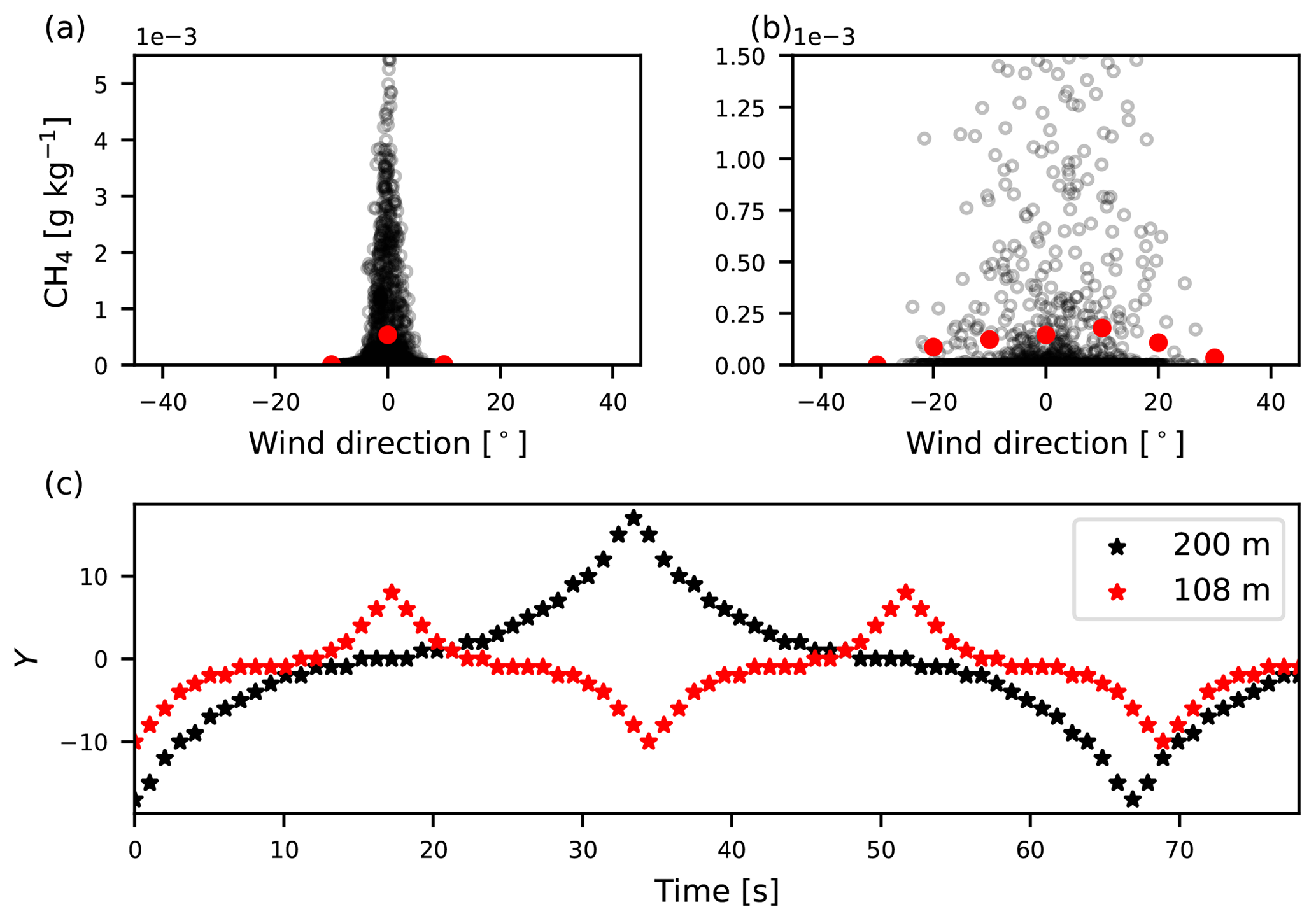
Figure 1(a) Methane concentration plotted against the wind direction according to the OTM 33A protocol for the case where no meandering is imposed. (b) Methane concentrations against the wind direction with imposed meandering. Red circles indicate bin averages. Bins of 10∘ are used. (c) An example of the sampling pattern used to impose meandering for two distances from the source.
The sampling was performed on an angle of around the plume centerline in the y direction. This angle was chosen in order not to sample outside of the plume. The instantaneous wind direction measured at each sampled point was added to the sampling angle. We move the location at which we record the sample back and forth between the plume edges, with a denser sampling close to the centerline, as shown in Fig. 1c (see Appendix A). Note that we impose larger values of Y when we sample further downwind of the source. Figure 1b shows the resulting OTM 33A concentrations after we sampled the plume with the additional meandering.
We have sampled the plume at four downwind distances that fall into the proposed range ( m; Edie et al., 2020). The samples were taken at m from the source. All three plumes were sampled at the height of their release (i.e., [0, 60, 190] m) with the frequency of 1 Hz for a duration of 30 min. Each plume was sampled 20 times with a time delay of 60 s between each sample to achieve reliable statistics.
3.3.2 Simulating car sampling
The sampling of the plume mimicking the car movements was performed in a similar manner to OTM 33A measurements. The concentration measurements were taken perpendicularly to the mean wind over the whole width of the domain (1536 m). The measurements were taken at the height of the release for each of the three emission heights and at eight downwind distances from the source, m.
Firstly, we have recorded instantaneous-plume transects over the y direction, i.e., mimicking an infinitely fast car. These instantaneous samples are used as a benchmark for plume measurements taken with realistic car speeds. We have taken 70 sets of measurements, each consisting of 100 plume transects, to gather statistics. The time delay between each set of measurements was taken as 10 s. The transects have also been sampled with a 10 s delay in between them. Secondly, to study the possible influence of driving speed on the source strength estimations, we have sampled the plume with two different car speeds, m s−1, with a sampling frequency of 1 Hz. The 1 Hz frequency represents the highest temporal resolution available from our simulation. As with the instantaneous-plume transects, we recorded 70 sets of 100 plumes, with a time delay of 10 s between sets and individual plumes.
To study the influence of atmospheric variability on the source strength estimation when using the Gaussian plume model, we averaged plumes in each of the 70 sets for each sampling strategy. The averaging was performed such that the resulting plume ( is the position on the y axis) is an average of t () previous plumes. In this way, we transformed each set of turbulent plumes into a set of averaged plumes. The first element is a single, non-averaged plume, and the last plume is an average of 100 plumes.
3.4 Statistical properties of the plumes
To further our understanding of the processes that govern plume dispersion close to and far from the source, plume dispersion can be subdivided into two processes. The first process (relative dispersion) is mixing by the turbulent eddies with a size smaller than or comparable to the size of the plume. The second process (meandering) is the displacement of the plume center of mass by the turbulent eddies that are larger than the size of the plume (e.g., Dinger et al., 2018).
To separate the influence of plume meandering from the influence of relative dispersion on the total plume growth, we can define relevant plume metrics in an absolute coordinate system (i.e., in relation to the ground) and a relative coordinate system (i.e., dispersion around an instantaneous center of mass). First, the center of mass of the instantaneous plume relative to the surface, zm, on its y–z transect is defined as
An ensemble average over many such instantaneous plumes will be equal to the center of mass of the time-averaged plume . Next, different metrics that measure plume displacement from its center of mass are defined. First, the absolute fluctuation z′ is the displacement of an in-plume particle from the mean center of mass . Second, the relative fluctuation is the displacement of an in-plume particle from the instantaneous-plume center of mass zm. Third, is the displacement of the instantaneous-plume centerline from the mean plume center of mass. These three metrics relate to each other as
Now the vertical plume widths, stemming from the two dispersion processes σz,meand (meandering) and σz,mix (mixing) are defined as
A similar expression applies to the total plume spread σz,tot around the mean center of mass zm:
where
Similar expressions apply to dispersion in the y direction.
4.1 Velocity and mean plume statistics
As a first step, the velocity statistics from the LES are validated against wind tunnel measurements presented in Nironi et al. (2015). The statistics are obtained as time (60 samples over 1 h of simulation) and horizontal (over the whole domain) averages. Figure 2a shows discrepancies between the non-dimensional wind speeds in the experiment and the LES. The wind speed at the top of the boundary layer in the LES is 4.9 m s−1, which is very close to the value of 5 m s−1 presented in Nironi et al. (2015). However, the friction velocities, u*, have values of 0.163 and 0.185 m s−1 in the LES and the experiment, respectively. As a result, the mean wind speeds differ when normalization with u* is used. Another possible reason for the discrepancies is the so-called overshoot of the mean wind in LES, which has been addressed previously (e.g., Brasseur and Wei, 2010; Ardeshiri et al., 2020). Overshoot in LES has been found to depend on the subgrid-scale (SGS) model, grid aspect ratio, grid resolution, and wall model. Despite the slight discrepancy in the mean wind, very good agreement is found between the wind speed variances (Fig. 2b) and covariances (Fig. 2c). Very good agreement is found for the triplet correlations as well (Fig. 2d). Ardeshiri et al. (2020) also reproduced the Nironi et al. (2015) case using LES and presented very similar results.
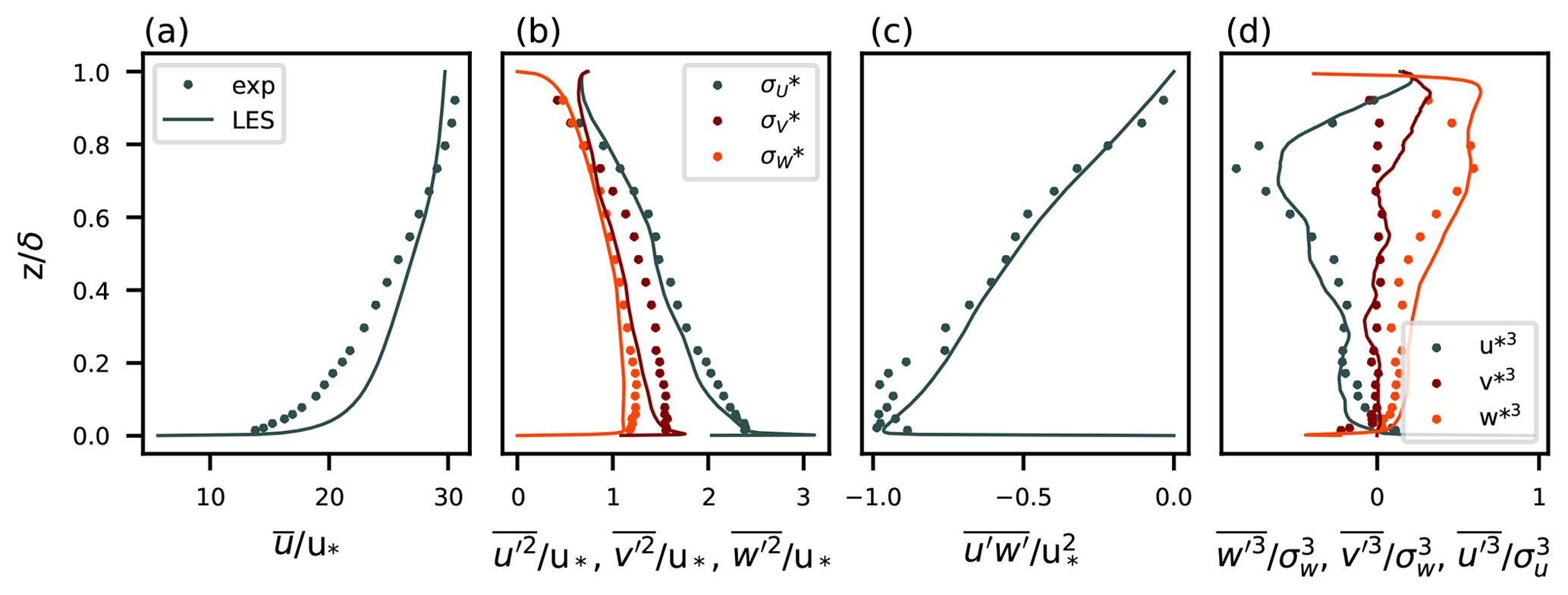
Figure 2Vertical profiles of non-dimensional velocity statistics and comparison with the Nironi et al. (2015) data. (a) Mean longitudinal wind speed. (b) Variances of three wind components. (c) Reynolds stress. (d) Triplet correlations.
Following the good agreement of the higher-order velocity statistics, we expect that the mixing of the plume in the cross-wind directions is well represented in the LES. The longitudinal mean wind affects the advection of the plume, i.e., the time the plume spent in the atmosphere being mixed by the turbulent eddies. Consequently, the statistics of the Nironi et al. (2015) plumes and the LES plumes cannot be compared at the same downwind distances. They can, however, be compared at the same effective distances from the source x*, defined as the downwind distance x scaled with one eddy overturn distance X:
where T is the characteristic eddy overturn time, is the mean wind speed, u* is the friction velocity, and δ is the boundary layer height. The downwind distance xLES at which the LES plume has spent an equal amount of “mixing time” compared to the Nironi et al. (2015) plume (xN) is
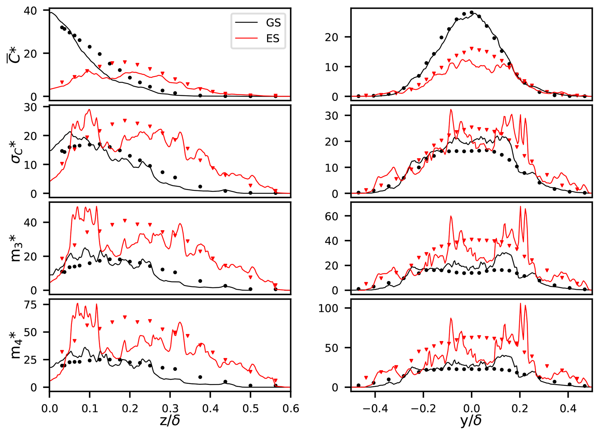
Figure 3Vertical (left column) and horizontal (right column) profiles of the first four statistical moments of plume concentration. Lines denote LES results, and symbols are corresponding results from Nironi et al. (2015). GS (black) denotes the source emitted at 0.06δ and ES (red) the source at 0.19δ. The transects are taken at xN = 2.5δ for the experiments. The corresponding values for xLES are 4.5 and 4.2δ for GS and ES, respectively.
Figure 3 shows a comparison of the first four statistical moments of the mean plume concentrations at the distance xN = 2.5δ. The moments are calculated over the horizontal and vertical plume transects at the height of the release and the y position of the source, respectively. The comparison is shown for the plumes released at 0.06δ and 0.19δ. The moments have been normalized (denoted by superscript *) with the plume emission rate Q (g s−1), free-stream velocity u∞ (m s−1), and the height of the boundary layer δ; e.g., is the normalized mean plume concentration. The mean plume profiles (Fig. 3 first row) show very good agreement over both transects: peaks of concentration and the plume width are well captured in the LES. The variances for the sources at 0.19δ (Fig. 3 second row) also show very good agreement. For the plume emitted closer to the ground, the variances agree well with the experiment at the edges of the plume but are higher in the LES at the plume centerline. The same can be observed for the other two moments shown here, the skewness and kurtosis (Fig. 3 bottom two rows). Note here that, for higher moments, LES curves do not show the same smoothness that is visible in the experiment despite the 600 samples used to calculate the average.
To give the reader an intuitive understanding of the spatial distribution of the plumes, Fig. 4 shows instantaneous x–z cross-sections of the three simulated plumes at the y position of the source (ys). The lowest plume stays relatively close to the surface and slowly mixes upwards with the increasing distance from the source. The middle plume stays compact around the emission height for a relatively short time before it is transported towards the surface. In contrast, the highest plume stays elevated for a considerable distance from its source (≈ 3000 m) before it is transported to the surface. While elevated, the highest plume exhibits highly meandering behavior: the spread of the plume around its instantaneous center of mass is narrow and is transported and broken up by larger eddies.
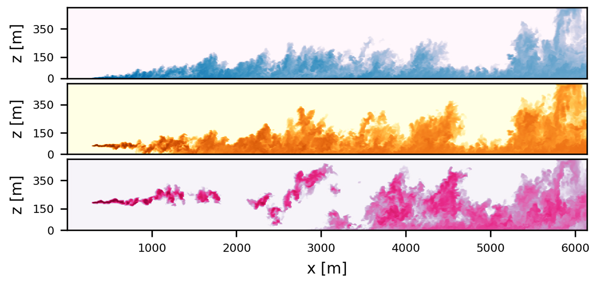
Figure 4Snapshot of x–z transects of the three plumes taken through the plume centerline. Blue, orange, and pink correspond to emission heights of 0, 60, and 190 m, respectively.
To illustrate these meandering motions, Fig. 5 shows 100 instantaneous y transects taken at emission height for each plume, separated by 24 s and at 1248 m from the source. Clearly, enhanced variability is found for the highest plume. Large eddies do not cause mixing close to the surface, and dispersion at this level is predominantly caused by diffusive processes. Furthermore, the lowest plume exhibits higher mean concentrations, which can be attributed to the lower mean wind speed close to the ground (Fig. 2a).
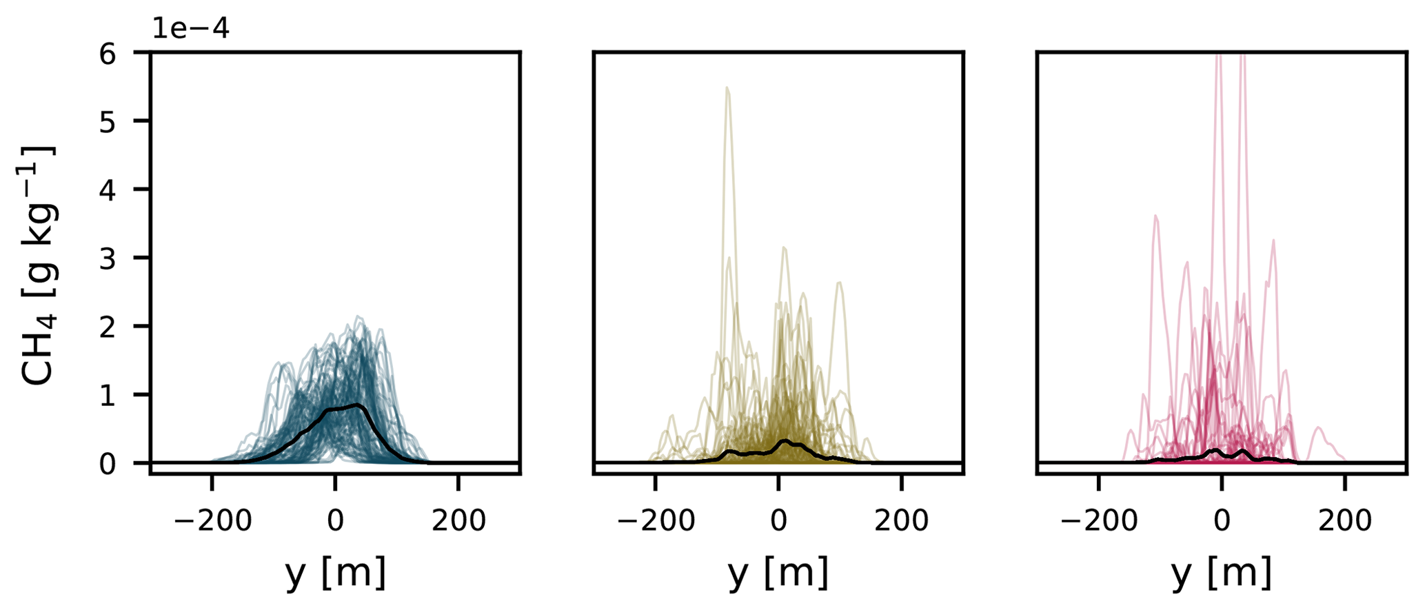
Figure 5Example of 100 instantaneous transects from three plumes, taken at the emission height of the respective plumes, at a distance of 1248 m from the source. The mean of the 100 plumes is shown in black. Blue, brown, and pink correspond to emission heights of 0, 60, and 190 m, respectively.
4.2 Structure of the time-averaged LES plume
The Gaussian plume model is a solution to the stationary advection–diffusion equation (Seineld, 1986) and can be interpreted as a time average of an infinite number of plume realizations. Therefore, by time averaging the LES plume over a large number of time steps, a Gaussian plume shape is expected. Figure 6 shows the time-averaged LES plumes in the x–z plane at the y position of the releases (ys = 0 m). Figure 6 also shows the edges of the plumes and the plume centerline (see Sect. 3.4). For comparison, the edges of a Gaussian plume σz,Briggs for stability class D defined by Eq. (2) are given.
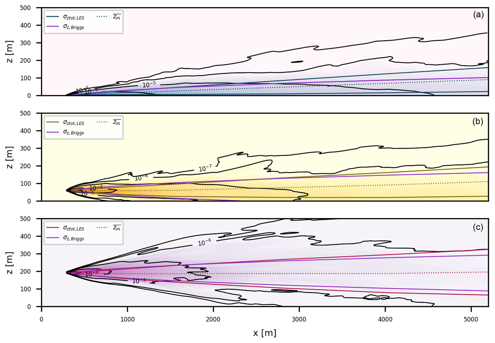
Figure 6Time-averaged x–z cross-section of the LES plume at (a) 0 m, (b) 60 m, and (c) 190 m height. The concentration fields are averaged over half an hour. The isolines connect the areas with the same concentration shown here (in g kg−1). Also plotted are the plume edges of the Gaussian plume (assuming Briggs diffusion coefficients) and the LES plumes. Centerlines are plotted as dashed lines.

Figure 7(a) Horizontal and (b) vertical plume width as a function of downwind distance from the source. Plume widths are shown for all three release heights as well as plume widths calculated using Briggs (Eq. 2).
Firstly, it can be observed that mean plume centerlines behave differently depending on the release height. For the highest release height (Fig. 6 bottom) the mean plume centerline stays at the emission height irrespective of the downwind distance from the source. Conversely, the plume centerline is lifted from the surface for the source at 0 m (Fig. 6 top) and at 60 m (Fig. 6 middle). This is a consequence of the vertical velocity field that is positively skewed at the lower heights (not shown). As a result, there are large areas of slowly sinking motions with occasionally strong upward ejections lifting the mean centerline position. Secondly, the lowest plume shows clear discrepancies in the lines that outline the plume edges in the Gaussian plume model and the LES. The Gaussian plume model only accounts for the effects of vertical mixing through the vertical dispersion coefficient, σz. Consequently, the plume centerline always remains at the emission height. Lastly, for the highest emission height, the widths of the Gaussian plume and the highest LES plume only start to diverge far from the source. For the two lower emission heights, the differences between the plume widths are larger. This is better illustrated in Fig. 7b. Here, σz values from Briggs and the 190 m release height are similar to those approximately 1000 m downwind of the source before they start to diverge. The slower vertical dispersion of the two lower plumes is also clearly visible. LES therefore indicates that vertical dispersion coefficients should be height dependent to capture changes in the wind regime with height. In contrast, horizontal dispersion coefficients (Fig. 7a) show very little variation with changing release height but are much smaller than the Briggs Gaussian plume coefficients. The small dispersion in the y direction can be attributed to the lack of the large-scale forcing in our simulation or the absence of eddies larger than the domain size (1536 m). We dictated the meandering part of dispersion in the horizontal direction (see Sect. 3.3.1).
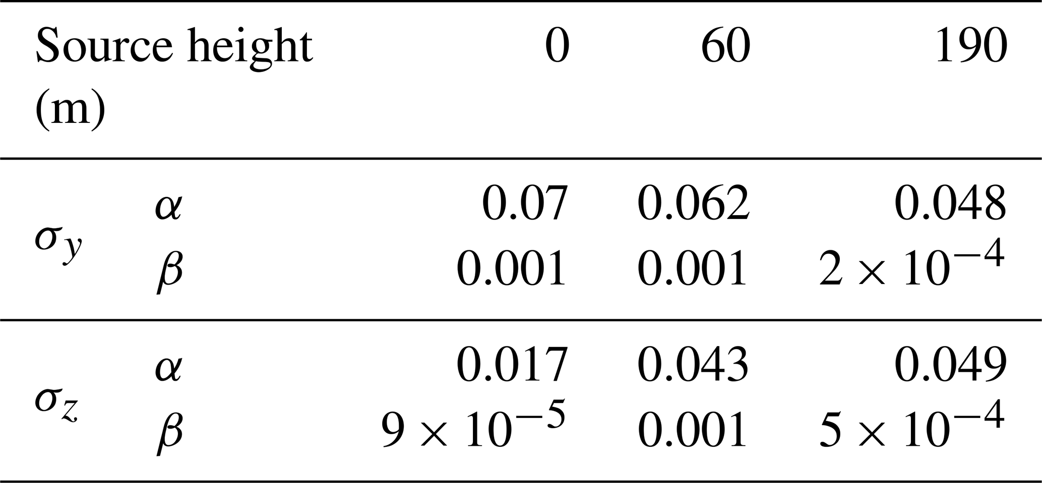
To mimic the Gaussian plume growth in both directions with Eq. (2), Table 1 gives the optimized coefficients that lead to a match with the LES plumes. These coefficients will be used in Sect. 4.3.1 for comparison to the dispersion coefficients from the look-up tables used in OTM 33A.
Table 1Coefficients of horizontal and vertical plume dispersion (Eq. 2) fitted for LES plumes with different source heights. remains unchanged from Eq. (2).
Now we move on to use the LES results to evaluate two techniques to infer the source strength from downwind concentration measurements: OTM 33A and the inverse Gaussian model using drive-bys.
4.3 OTM 33A
In order to obtain Gaussian profiles of mean concentrations (see Fig. 1), we followed the sampling procedure described in Sect. 3.3.1 to mimic plume meandering. Source strength estimates using OTM 33A at four different distances from the source ( m) are shown in Fig. 8. The tracer concentrations were recorded over 20 min (1200 data points). To obtain measurement ensembles, the sampling was repeated 20 times, as described in Sect. 3.3.1.
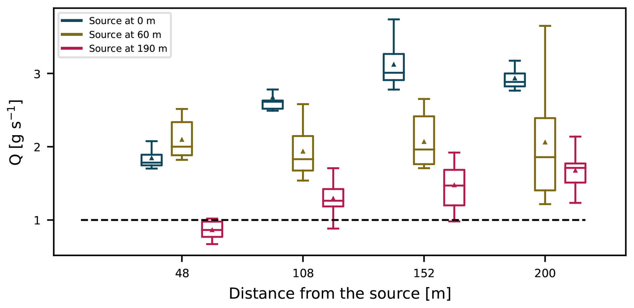
Figure 8Estimates of the source strength using OTM 33A for the emission heights 190, 60, and 0 m at four different distances. Boxes show the interquartile range, while the whiskers span from the 5th to 95th percentile of the data and show the mean and median. The dashed line refers to the true source strength used in the LES.
The most striking result is that for nearly all emission heights OTM 33A overestimates the source strength. Uncertainties generally increase slightly with increasing distance from the source. Only for the 190 m source is the estimated source strength at the downwind distance of 48 m close to the true source strength. We found that this effect is caused by the way we introduce the source into the atmosphere. Instead of emitting the tracer as a point source, we use a Gaussian distribution to pre-disperse the source (see Sect. 3.1 and 3.2). In combination with the implemented meandering (Sect. 3.3.1), sampling close to the source coincidentally leads to plume dispersion similar to the dispersion of the OTM 33A-imposed Gaussian plume. Following this, we expect the different source sizes to have a different effect on the source strength estimation at distances very close to source. In future studies, it is recommended to quantify the effect of the prescribed source size on the source estimation using OTM 33A.

Figure 9Probability density functions of the instantaneous-plume centerline positions with respect to the plume emission positions (blue: 0 m; yellow: 60 m; pink: 190 m) in the y (left column) and z (right column) directions. Bins of 1.5 m are used.
Further away from the source and with lower emission heights, a general overestimation is found. The estimated source strengths using OTM 33A depend linearly on the dispersion parameters (Eq. 3). Consequently, too large dispersion parameters automatically lead to overestimated source strengths. The dispersion parameters used here were taken from the recommended look-up table (U.S. EPA, 2014). These values are based on the Pasquill–Gifford dispersion curves, just like the Briggs coefficients. As we have shown (Fig. 7a), these values are too large in the y direction compared to our LES dispersion calculation, explaining the overestimates. We have also shown that dispersion parameters in the z direction depend on the height of the source. While the differences in the z direction are not so pronounced, especially for the highest source (Fig. 7b), they also contribute to the error in estimates. At the closest distance from the source, the estimates for the two lower sources have larger errors compared to the highest source. There are several causes for this. Firstly, as previously discussed, the vertical dispersion coefficient for the highest plume has a better agreement with the Briggs dispersion coefficient at distances close to the source. Secondly, according to the OTM 33A protocol, the concentrations should be recorded at the plume centerline, which is assumed to be at emission height. However, we found that for different emission heights the instantaneous plumes' centerline positions behave differently. Figure 9 shows the probability density functions (pdf's) of instantaneous=plume centerline positions relative to the y and z position of the source (ys,zs). In the z direction, the pdf's have longer tails for values above the emission height (positive skewness). In contrast, the lowest plume lifts off the ground with distance from the source. With downwind distance, the displacements from the emission height grow as do the errors in the source strength estimates. In the y direction, the highest and the lowest plumes have slightly positively skewed pdf's relative to the emission point. The skewness in the middle plume is even more pronounced. This, in combination with the plumes still being very narrow, results in plumes being sampled at their edges, which leads to high estimation errors. The error also depends on the distance from the source as the height of the plume median is not constant. Further downwind this effect is less pronounced since the plumes become wider and sampling slightly out of the plume's median position still characterizes the plume well.
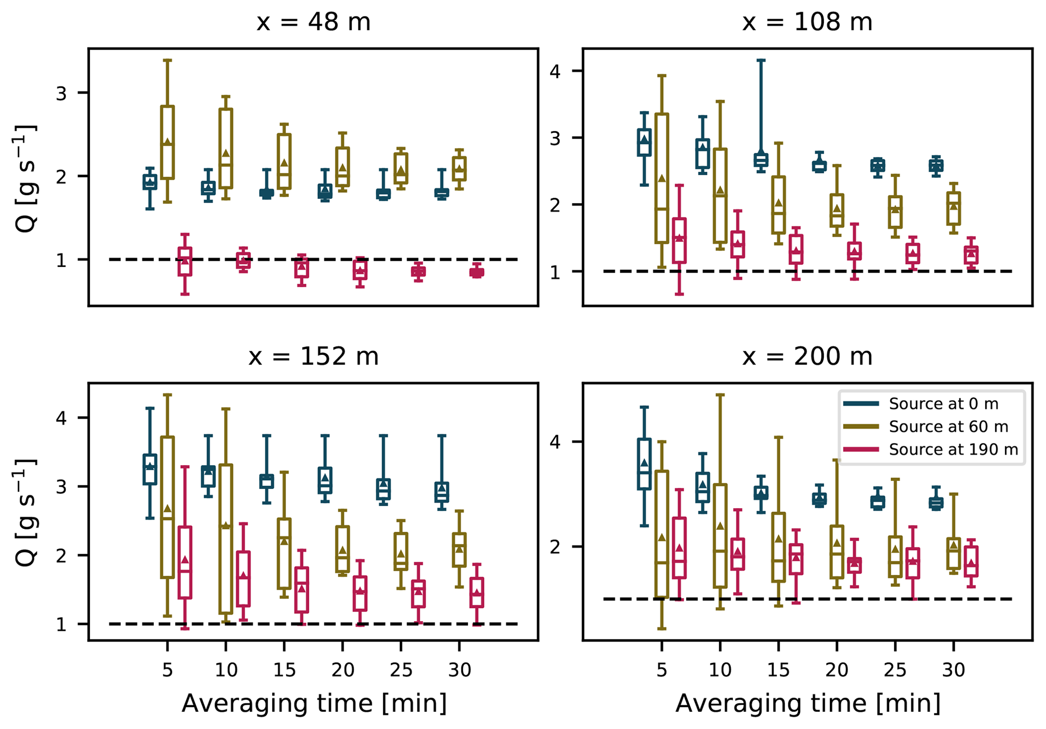
Figure 10Source estimation using OTM 33A for four different distances from the source and for different averaging times. Boxes show the interquartile range, while the whiskers span from the 5th to 95th percentile of the data and show the mean and median. The dashed lines refer to the true source strength used in the LES.
Next, we study the influence of the averaging time on the source estimation. In Fig. 10 we show source estimates for six different averaging times at four sampling distances. The estimates for all emission heights show similar behavior. Averaging for 20 min leads to smaller estimation errors for all three sources. Convergence of the error becomes slower with increasing distance from the source for the two higher sources. The lowest source had a small estimation error even for short averaging times at most downwind distances. From Fig. 5 it is visible that the lowest plume shows little variability even when measured much further from the source (1248 m in Fig. 5) than OTM 33A suggests.
Lower variability in estimations closer to the source can be attributed to a short dispersion time. As previously mentioned, the plume's dispersion is a combination of relative dispersion around the instantaneous center of mass and the meandering motions. At very short distances from the source the plume will retain the initial source shape until it is sufficiently mixed by the relative motions. Even with the added meandering that we implement (see Sect. 3.3, Fig. 1), the sampled plume resembles the shape of the source. Consequently, until the plume is sufficiently mixed by smaller eddies, the variability between OTM 33A experiments used to produce the boxplots in Fig. 10 is not large. The increase in uncertainty with distance is related to the increase in the plume size.
4.3.1 Structure of the plume close to the source
To study the structure of the plumes close to the source, we analyze the plume statistics following the approach described in Sect. 3.4. To that end, we investigate the two processes responsible for plume dispersion (mixing and meandering) separately. The effect of turbulent mixing on the plume (σmix, as defined in Sect. 3.4, Eq. 9) is isolated by averaging the 3600 plumes after aligning them according to their (displaced) center of mass in the y and z directions. Figure 11 shows these time-averaged plumes, both aligned and non-aligned (meandering included) in the y direction at four distances from the source for the largest emission height. The figure also depicts Gaussian functions fitted to the aligned and non-aligned plumes, calculated according to Eq. (9) (σmix) and Eq. (10), respectively. For reference, the recommended OTM 33A Gaussian dispersion is also plotted.
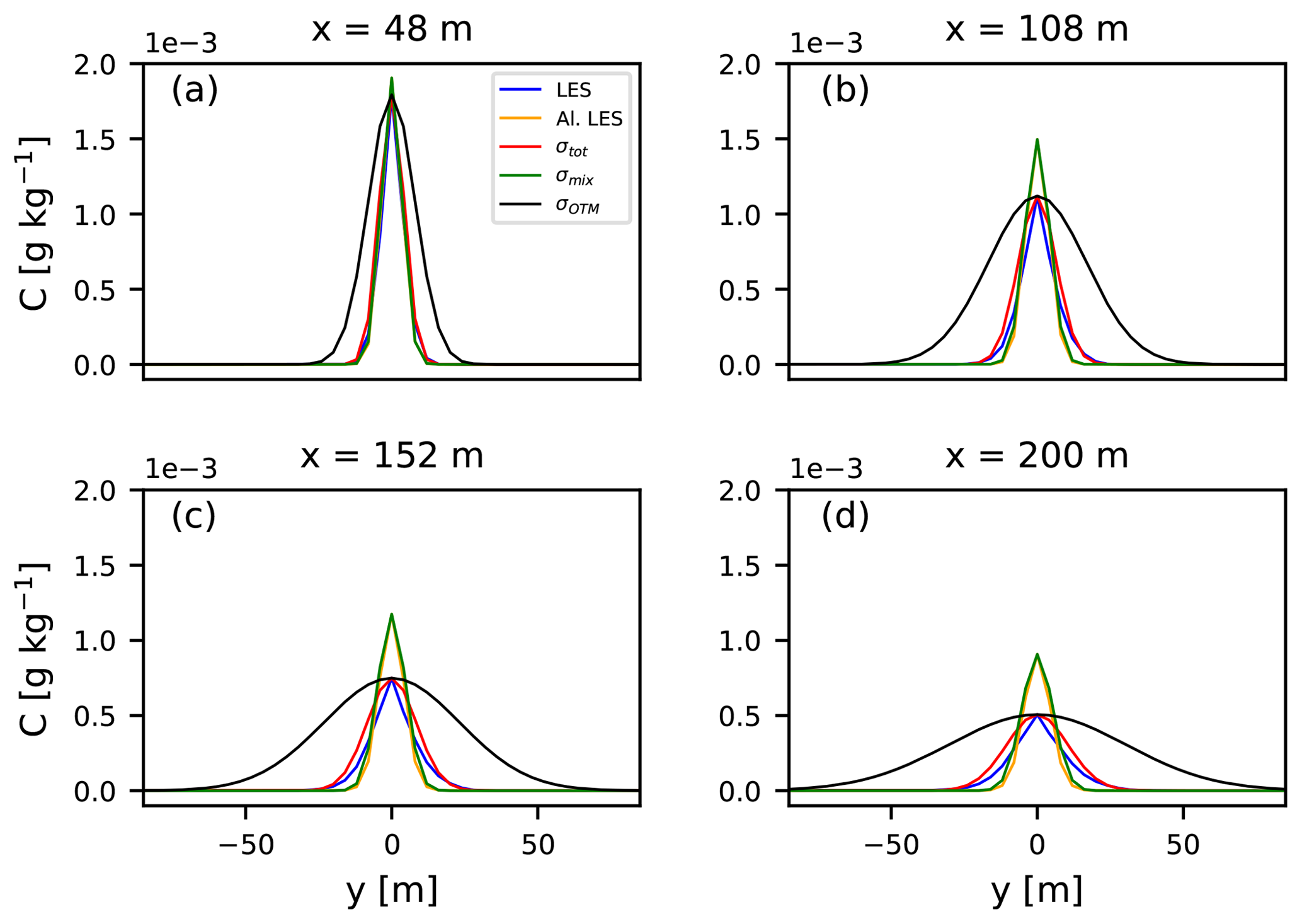
Figure 11Time averages of instantaneous plumes (blue) on the plume centerline and the instantaneous plumes aligned according to their centers of mass (orange), in the y direction. Fitted through them are Gaussian functions with 1 standard deviation of their width σi (m) (green: mixing; red: total). For reference, we show Gaussian functions fitted to the maximum of the non-aligned plume with σ taken from OTM 33A (black). Emission and sampling heights are 190 m.
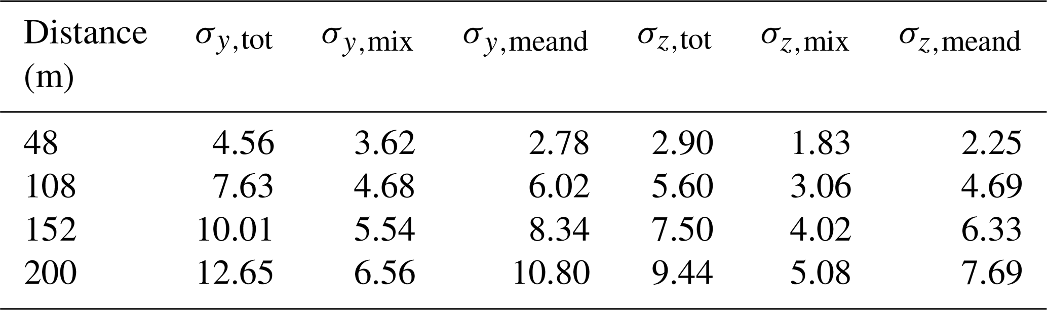
In general, the non-aligned Gaussian functions are wider due to the meandering effect of the larger eddies that has been implemented (Eq. 9, σmeander). As before, we find that the OTM 33A dispersion coefficients are significantly larger than the time-averaged plumes. For the closest transect at 48 m, the tails of the non-aligned plume are very short and very similar to those of the aligned plume. This supports the observation that close to the source the plume is still very narrow and is not moved much by the larger-sized eddies or dispersed around its centerline by the smaller ones. The shape of the plume at 48 m is determined by the shape of the sources (Sect. 3.1). Further downwind the difference between the aligned and non-aligned plumes grows, which indicates that the plume is being moved around significantly by larger eddies. At 200 m from the source, the aligned plume is still compact, which indicates that dispersion by small eddies is a slow process. The same behavior can be observed for the z direction (not shown). The values of the derived dispersion coefficients are given in Table 2.
Table 2Dispersion coefficients σ (in m), obtained by using the definitions presented in Sect. 3.4, for the plume emitted at 190 m.
We tested OTM 33A with the dispersion coefficients derived from the LES. Understandably, the source estimates improve considerably compared to OTM 33A, but we still find estimation errors of up to ≈ 40 % (not shown). We argue that these errors are caused by the vertical displacement of the plume during transport (see Fig. 6). As previously mentioned, one of the assumptions of OTM 33A is that the measurements are taken at the emission height. However, very close to the source the mean plume position, emission height, and the mode of the instantaneous-plume positions do not necessarily coincide (Fig. 9). This is a likely consequence of the skewed vertical velocity field discussed previously in Sect. 4.2. On top of that, we found that the pdf of the instantaneous-plume positions is also slightly skewed in the y direction (Fig. 9), which contributes to the overall error.
In conclusion, we find that the errors associated with OTM 33A are sizable. One source of errors is associated with the assumed dispersion coefficients, which were found to be too large compared to LES. Other sources of errors are related to assumptions made in the Gaussian plume model.
4.4 Source strength estimation from car measurements
Now we move to the analysis of more dispersed plumes that are sampled further away from the source (>200 m). Figure 12 shows results of car measurements taken perpendicularly to the mean wind and at plume emission height for all three sources. Estimates were made following the inverse Gaussian method described in Sect. 2.3. The Gaussian plume model employed (Sect. 2.1) uses Briggs dispersion coefficients and the mean wind speed in the x direction at the height of the release. Estimates are shown for transects taken by an infinitely fast car. The transects are taken according to the sampling procedure described in Sect. 3.3.2. If only one transect is made, the estimated source strength shows a large spread for all distances, with estimates being up to 4 times larger than the real source strength. The medians show a negative bias, indicating that a large fraction of the plumes have relatively low concentrations, and a few plumes exhibit (very) large concentrations. This result is expected, since the most concentrated part of the plume is moving over a 2-D (y–z) plane (e.g., Fig. 5). The probability of sampling this part of the plume with a 1-D transect is less likely. When the source strength is calculated using averaged plumes (see Sect. 3.3.2), it becomes more likely to estimate the emission strength accurately. This is due to turbulent fluctuations in the plumes being averaged out. As a result, the averaged plume becomes more Gaussian as more transects are included in the average. For instance, the spread drops by ≈ 50 % if 10 transects are averaged. These results are in line with the findings of Caulton et al. (2018), who proposed averaging over at least 10 transects. As opposed to the estimations from the two higher plumes, the estimations from the lowest plume exhibit very little variability. As we have discussed in relation to Fig. 5, large eddies do reach the surface but merely displace the plume, and plume dispersion at this level is predominantly caused by small-eddy processes.
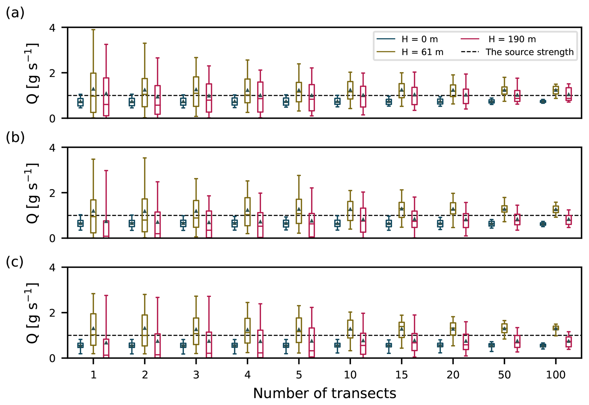
Figure 12Estimates of the source strength from instantaneous-plume transects for all three emission heights. Boxes show the interquartile range, while the whiskers span from the 5th to 95th percentile of the data and show the mean and median. Distances from the source are (a) 200 m, (b) 624 m, and (c) 1248 m.
In contrast to OTM 33A, the estimated source strengths converge to the true value with sufficient averaging time using car transects. This is due to the fact that the car transect method calculates the mass flux of the tracer by integrating over the (assumed) Gaussian profile. The flux of the mass through any given y–z plane in both models is conserved and equal, irrespective of the width of the actual plumes. Note here that the LES plume in our analysis is still much narrower in the y direction compared to the Gaussian plume. In the vertical direction, the LES plume width is comparable to the Gaussian one (Fig. 7). If this were not the case, the analysis would give incorrect source estimates since a different displacement of mass in the vertical would lead to a different horizontal line integral.
It can be seen that the estimations, depending on their distance from source, converge to a slightly different value than the true source strength. This can be related to the position of the plume centerline and the plume mode discussed in Sect. 4.2 and 4.3. For the LES plumes the position of the mode varies with the distance from the source, while in the Gaussian plume model the plume centerline does not diverge from the emission height. This mismatch in the two models effectively means that two plumes with different emission heights are being compared. When the emission height in the Gaussian plume model is adjusted to match the height of the LES plume mode for a certain downwind distance, the estimation error disappears.
Lastly, we have repeated the analysis of source strength estimations sampled outside of the plume centerline (not shown). Notably, the closer the plume is sampled to its edge, the more transects are needed for the estimates to converge to the true value. This was an expected result since at its edge the plume shows the greatest variability, as shown in previous studies (e.g., Dosio and de Arellano, 2006; Gailis et al., 2007; Ardeshiri et al., 2020).
To study the convergence of the results, Fig. 13 shows standard deviations of the source strength estimation for the plume emitted at 190 m. The standard deviations are shown for the first 40 plumes at eight different distances from the source. After ≈ 10 transects, the standard deviation decays with the inverse square root of the number of averaged plumes. This confirms that all transects through the plume are independent and that the time difference between the samples was not too short. We also studied the influence of driving speed through the plume for cars driving slowly (4 m s−1) and fast (12 m s−1) but found no significant difference in results from transects taken by infinitely fast cars.
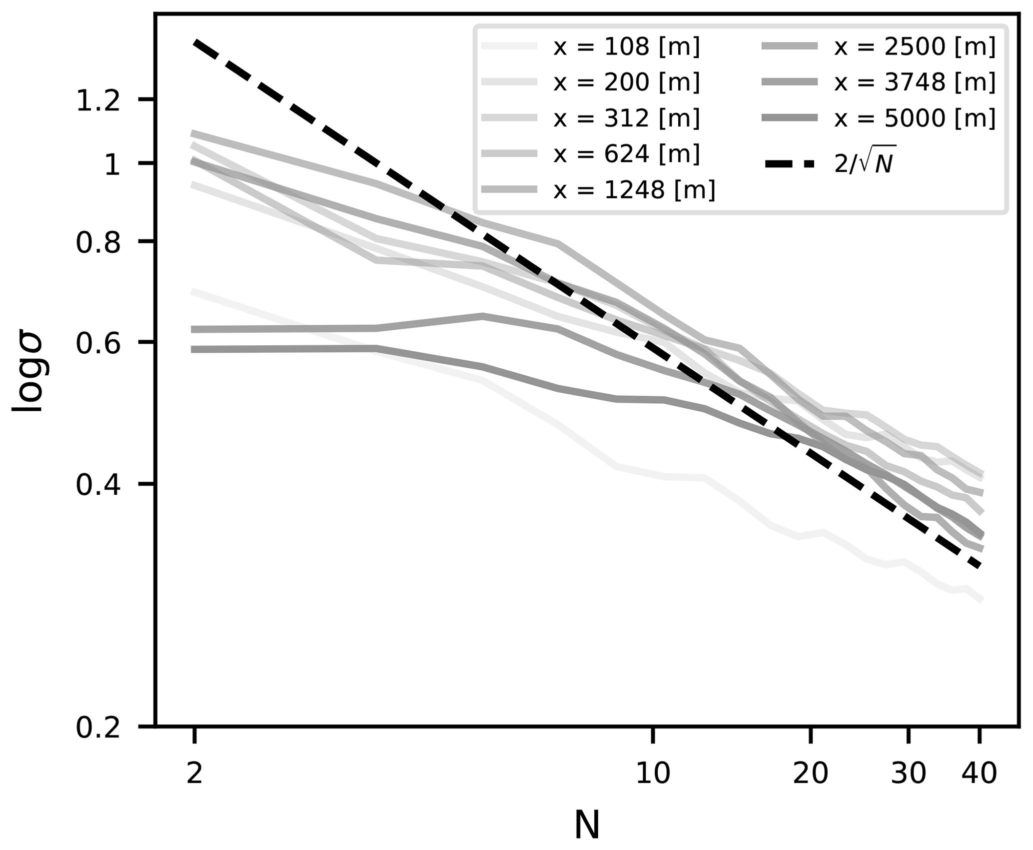
Figure 13Standard deviation of the source strength estimates with increasing sample size for eight different distances from the source. The emission and sampling heights are 190 m.
In this study, we performed a large-eddy simulation (LES) of point source plumes released into a neutrally stable, homogeneous, and statistically stationary turbulent flow over a flat terrain. Simulations were performed following the laboratory experiment by Nironi et al. (2015) of point source plume dispersion in a turbulent channel flow. Point sources were placed at three altitudes, m. We sampled our numerical plumes according to two measurement protocols that aim to estimate point source strengths with the aid of the Gaussian plume formalism. The aim was to quantify the uncertainties in the drive-through method and OTM 33A.
We found that the time-averaged LES plume has a Gaussian shape but that the dispersion rate of the plume in the y direction is slower compared to a Gaussian plume with the Briggs dispersion coefficients representative of a neutral boundary layer (e.g., Griffiths, 1994). One of the reasons why our y dispersion is smaller might be the lack of large-scale variability in our simulation, which is instead forced by a constant gradient pressure force. In the vertical, the discrepancies between the Briggs coefficients and the LES plumes were less pronounced. However, for smaller release heights, the mean plume centerline is displaced in the vertical, a feature that is not captured in the standard Gaussian plume dispersion coefficients. The rise of the plume centerline downwind of the source is caused by the nature of the boundary layer turbulence, which has large areas of slow sinking motions and small areas with stronger upward motions.
Application of OTM 33A to our simulated plumes showed that we tend to overestimate the source strength by ≈ 50 %–200 %. Previous studies (Edie et al., 2020) showed a 2σ uncertainty in the source strength of ±70 % but without a bias. The significant overestimation in our results is a direct consequence of the OTM 33A formalism in which the derived source strength depends linearly on the dispersion coefficients. Coefficients based on Pasquill–Gifford dispersion curves (e.g., U.S. EPA, 2014; Seineld, 1986) and Briggs coefficients (Griffiths, 1994) are both too dispersive compared to the LES simulation.
By aligning and averaging the plumes according to their center of mass, we were able to show that, at distances smaller than ∼ 150 m from the source, the plume shows a shape that is similar to the source shape, i.e., a very narrow Gaussian shape. The aligned and non-aligned plumes are similar, indicating that the plume is moved very little from its center of mass by larger eddies (meandering) even though OTM 33A accounts for that. From Fig. 3 this is most obvious for the plume at 48 m. Further downwind the height of the aligned plume peak becomes smaller, indicating the dispersion in the z direction also plays an important role. Nevertheless, if the dispersion coefficients derived for the individual LES plumes are used in combination with OTM 33A, significantly smaller errors are found. Another source of the errors in OTM 33A is the position of the plume in relation to its centerline. The method assumes that the plume centerline position, emission height, and the mode of the centerline position coincide. We were able to show that this is not necessarily true and that this mismatch leads to additional uncertainties in the source estimation.
We also simulated drive-bys at distances of up to 1248 m from the source. The plumes were sampled simulating different car speeds with a sampling frequency of 1 Hz to mimic realistic field conditions. We used the inverse Gaussian model (IGM) method to derive the source strength, with the mean wind taken from the LES at release height and using Briggs dispersion coefficients. We found that the correct source strength is estimated if the result is averaged over a sufficient number of different realizations. To estimate the source strength within ≈ 40 %, we recommend averaging over at least 15 drive-bys. This supports the findings from Caulton et al. (2018), who recommended at least 10 transects. Our results show no significant influence of the driving speed on the source strength estimation. The IGM method is insensitive to errors in y dispersion because the method depends on the line integral in the y direction. We found, however, that a mismatch between the vertical centerline position of the plume and the emission height does produce an error in the source estimation. This error can be corrected by adjusting the height of the Gaussian plume to match the simulated plume centerline.
The plumes studied here were emitted into the neutral channel flow as this is the most canonical case of the atmospheric turbulence. A similar study should be performed for unstable and stable conditions. Based on our findings, we expect additional variance of the plume under unstable conditions because of buoyancy effects producing additional turbulence. Conversely, for a stable atmosphere, we expect that a shorter averaging time (fewer plume transects) would be needed to achieve 40 % accuracy.
Our study has shown some of the advantages and drawbacks of two commonly used measurement techniques for source strength estimations. To arrive at our conclusions, we used the neutral channel flow experiment that resembles the purely shear-driven turbulence in an atmospheric surface layer. In this setting, the possible errors in the estimations are expected to be minimized since the turbulence is well understood and the Gaussian plume model is logically derived. A next step would be to repeat this study for different stability conditions in an idealized setting such as this, as in for example the LES experiment performed by Xiao et al. (2021) of plume dispersion in a stable boundary layer, or to re-create real field conditions (Ražnjević et al., 2022). With constantly improving numerical techniques, LES is capable of reproducing real meteorological conditions encountered in the field. Combined with improving observational techniques, this approach is expected to lead to better estimates of source strengths.
Here we describe the plume sampling procedure used to mimic the large-scale plume meandering necessary for OTM 33A.
If we define 0 as the left edge of the plume and 1 as the right edge, we can define a function of time, ζ, that oscillates between 0 and 1 with a uniform step, essentially mimicking forward and backward motions through the plume. In order to achieve denser sampling around the centerline, we re-define our sampling function in a way that gives us the relative position between −0.5 and 0.5, , as
where is the grid point at which the sample was taken at the time step i. Factor A determines the density of the sampling points around the centerline, and we have set it to A=3. We can then convert this array into dimensional units to find the position, Yi, at which the sample is taken by adapting the relative position, , to the actual plume width, L, as is shown in Eq. (A2):
The acquired sampling pattern for two distances from the source is shown in Sect. 3.3.1, Fig. 1a. We applied the sampling strategy at m from the source. With the assumed θ=15∘, the width over which plumes were sampled was m for each of the distances from the source, respectively.
The simulations were performed using the MicroHH model available at https://doi.org/10.5281/zenodo.822842 (van Heerwaarden et al., 2017b).
Data used in this paper came either from the simulations themselves (description of setup and sampling in the text) or from the experiment published in Nironi et al. (2015).
AR, CvH, and MK designed the research. AR performed the simulations and all analyses and wrote the manuscript in close collaboration with CvH and MK.
The contact author has declared that neither they nor their co-authors have any competing interests.
Publisher’s note: Copernicus Publications remains neutral with regard to jurisdictional claims in published maps and institutional affiliations.
This project is part of the MEthane goes MObile – MEasurements and MOdelling (MEMO2) project. The authors acknowledge and thank Pietro Sallizoni and Massimo Marro for sharing their experimental data.
This project has received funding from the European Union’s Horizon 2020 research and innovation program (Marie Skłodowska-Curie grant agreement no. 722479). Maarten Krol received funding from the European Research Council (ERC) under the European Union’s H2020 research and innovation program (grant agreement no. 742798).
This paper was edited by Cléo Quaresma Dias-Junior and reviewed by two anonymous referees.
Andersen, T., Scheeren, B., Peters, W., and Chen, H.: A UAV-based active AirCore system for measurements of greenhouse gases, Atmos. Meas. Tech., 11, 2683–2699, https://doi.org/10.5194/amt-11-2683-2018, 2018. a
Ardeshiri, H., Cassiani, M., Park, S. Y., Stohl, A., Pisso, I., and Dinger, A. S.: On the Convergence and Capability of the Large-Eddy Simulation of Concentration Fluctuations in Passive Plumes for a Neutral Boundary Layer at Infinite Reynolds Number, Bound.-Lay. Meteorol., 176, 291–327, https://doi.org/10.1007/s10546-020-00537-6, 2020. a, b, c, d, e
Atherton, E., Risk, D., Fougère, C., Lavoie, M., Marshall, A., Werring, J., Williams, J. P., and Minions, C.: Mobile measurement of methane emissions from natural gas developments in northeastern British Columbia, Canada, Atmos. Chem. Phys., 17, 12405–12420, https://doi.org/10.5194/acp-17-12405-2017, 2017. a, b, c
Baillie, J., Risk, D., Atherton, E., O'Connell, E., Fougére, C., Bourlon, E., and MacKay, K.: Methane emissions from conventional and unconventional oil and gas production sites in southeastern Saskatchewan, Canada, Environmental Research Communications, 1, 011003, https://doi.org/10.1088/2515-7620/ab01f2, 2019. a
Baker, L. H., Collins, W. J., Olivié, D. J. L., Cherian, R., Hodnebrog, Ø., Myhre, G., and Quaas, J.: Climate responses to anthropogenic emissions of short-lived climate pollutants, Atmos. Chem. Phys., 15, 8201–8216, https://doi.org/10.5194/acp-15-8201-2015, 2015. a
Berman, E. S., Fladeland, M., Liem, J., Kolyer, R., and Gupta, M.: Greenhouse gas analyzer for measurements of carbon dioxide, methane, and water vapor aboard an unmanned aerial vehicle, Sensor. Actuat. B-Chem., 169, 128–135, https://doi.org/10.1016/j.snb.2012.04.036, 2012. a
Boppana, V. B. L., Xie, Z.-T., and Castro, I. P.: Large-eddy simulation of dispersion from surface sources in arrays of obstacles, Bound.-Lay. Meteorol. 135, 433–454, https://doi.org/10.1007/s10546-010-9489-9, 2010. a
Boppana, V. B. L., Xie, Z. T., and Castro, I. P.: Large-eddy simulation of dispersion from line sources in a turbulent channel flow, Flow Turbul. Combust., 88, 311–342, https://doi.org/10.1007/s10494-011-9356-x, 2012. a, b
Branford, S., Coceal, O., Thomas, T. G., and Belcher, S. E.: Dispersion of a point-source release of a passive scalar through an urban-like array for different wind directions, Bound.-Lay. Meteorol. 139, 367–394, https://doi.org/10.1007/s10546-011-9589-1, 2011. a
Brantley, H. L., Thoma, E. D., Squier, W. C., Guven, B. B., and Lyon, D.: Assessment of methane emissions from oil and gas production pads using mobile measurements, Environ. Sci. Technol., 48, 14508–14515, https://doi.org/10.1021/es503070q 2014. a
Brasseur, J. G., and Wei, T.: Designing large-eddy simulation of the turbulent boundary layer to capture law-of-the-wall scaling, Phys. Fluids, 22, 021303, https://doi.org/10.1063/1.3319073, 2010. a
Briggs, G.: Diffusion estimation of small emissions, NOAA, Atmospheric Turbulence and Diffusion Laboratory Contribution No. 79, 83–145, https://doi.org/10.2172/5118833, 1973. a
Cassiani, M., Bertagni, M. B., Marro, M., and Salizzoni, P.: Concentration Fluctuations from Localized Atmospheric Releases, Bound.-Lay. Meteorol., 177, 461–510, https://doi.org/10.1007/s10546-020-00547-4, 2020. a
Caulton, D. R., Li, Q., Bou-Zeid, E., Fitts, J. P., Golston, L. M., Pan, D., Lu, J., Lane, H. M., Buchholz, B., Guo, X., McSpiritt, J., Wendt, L., and Zondlo, M. A.: Quantifying uncertainties from mobile-laboratory-derived emissions of well pads using inverse Gaussian methods, Atmos. Chem. Phys., 18, 15145–15168, https://doi.org/10.5194/acp-18-15145-2018, 2018. a, b, c, d, e, f, g
Cimorelli, A. J., Perry, S. G., Venkatram, A., Weil, J. C., Paine, R. J., Wilson, R. B., Leeg, R. F., Peters, W. D., and Brode, R. W.: AERMOD: A dispersion model for industrial source applications. Part I: General model formulation and boundary layer characterization, J. Appl. Meteorol., 44, 682–693, https://doi.org/10.1175/JAM2227.1, 2005. a
Csanady, G. T.: Turbulent Diffusion in the Environment, D. Reidel Publishing Company, Dordrecht, 248 pp., https://doi.org/10.1007/978-94-010-2527-0, 1973. a
Cui, Y. Y., Henze, D. K., Brioude, J., Angevine, W. M., Liu, Z., Bousserez, N., Guerrette, J., McKeen, S. A., Peischl, J., Yuan, B., Ryerson, T., Frost, G., and Trainer, M.: Inversion Estimates of Lognormally Distributed Methane Emission Rates From the Haynesville-Bossier Oil and Gas Production Region Using Airborne Measurements, J. Geophys. Res.-Atmos., 124, 3520–3531, https://doi.org/10.1029/2018JD029489, 2019. a
Dinger, A. S., Stebel, K., Cassiani, M., Ardeshiri, H., Bernardo, C., Kylling, A., Park, S.-Y., Pisso, I., Schmidbauer, N., Wasseng, J., and Stohl, A.: Observation of turbulent dispersion of artificially released SO2 puffs with UV cameras, Atmos. Meas. Tech., 11, 6169–6188, https://doi.org/10.5194/amt-11-6169-2018, 2018. a
Dosio, A. and de Arellano, J. V. G.: Statistics of absolute and relative dispersion in the atmospheric convective boundary layer: a large-eddy simulation study, J. Atmos. Sci., 63, 1253–1272, https://doi.org/10.1175/JAS3689.1, 2006. a, b
Edie, R., Robertson, A. M., Field, R. A., Soltis, J., Snare, D. A., Zimmerle, D., Bell, C. S., Vaughn, T. L., and Murphy, S. M.: Constraining the accuracy of flux estimates using OTM 33A, Atmos. Meas. Tech., 13, 341–353, https://doi.org/10.5194/amt-13-341-2020, 2020. a, b, c, d
Foster-Wittig, T. A., Thoma, E. D., and Albertson, J. D.: Estimation of point source fugitive emission rates from a single sensor time series: A conditionally-sampled Gaussian plume reconstruction, Atmos. Environ., 115, 101–109, https://doi.org/10.1016/j.atmosenv.2015.05.042, 2015. a
Fritz, B. K., Shaw, B. W., and Parnell, C. B.: Influence of meteorological time frame and variation on horizontal dispersion coefficients in gaussian dispersion modeling, T. ASAE, 48, 1185–1196, https://doi.org/10.13031/2013.18501, 2005. a
Gailis, R. M., Hill, A., Yee, E., and Hilderman, T.: Extension of a fluctuating plume model of tracer dispersion to a sheared boundary layer and to a large array of obstacles, Bound.-Lay. Meteorol., 122, 577–607, https://doi.org/10.1007/s10546-006-9118-9, 2007. a
Gifford, F.: Statistical properties of a fluctuating plume dispersion model, Adv. Geophys., 6, 117–137, https://doi.org/10.1016/S0065-2687(08)60099-0, 1959. a
Griffiths, R. F.: Errors in the use of the Briggs parameterization for atmospheric dispersion coefficients, Atmos. Environ., 28, 2861–2865, https://doi.org/10.1016/1352-2310(94)90086-8, 1994. a, b, c
Hensen, A. and Scharff, H.: Methane emission estimates from landfills obtained with dynamic plume measurements, Water Air Soil Poll., 1, 455–464, https://doi.org/10.1023/A:1013162129012, 2001. a
Hensen, A., Groot, T. T., Van den Bulk, W. C. M., Vermeulen, A. T., Olesen, J. E., and Schelde, K.: Dairy farm CH4 and N2O emissions, from one square metre to the full farm scale, Agr. Ecosyst. Environ., 112, 146–152, https://doi.org/10.1016/j.agee.2005.08.014, 2006. a
Houweling, S., Krol, M., Bergamaschi, P., Frankenberg, C., Dlugokencky, E. J., Morino, I., Notholt, J., Sherlock, V., Wunch, D., Beck, V., Gerbig, C., Chen, H., Kort, E. A., Röckmann, T., and Aben, I.: A multi-year methane inversion using SCIAMACHY, accounting for systematic errors using TCCON measurements, Atmos. Chem. Phys., 14, 3991–4012, https://doi.org/10.5194/acp-14-3991-2014, 2014. a
Korsakissok, I. and Mallet, V.: Comparative study of Gaussian dispersion formulas within the Polyphemus platform: evaluation with Prairie Grass and Kincaid experiments, J. Appl. Meteorol. Clim., 48, 2459–2473, https://doi.org/10.1175/2009JAMC2160.1, 2009. a, b, c
Lan, X., Talbot, R., Laine, P., and Torres, A.: Characterizing fugitive methane emissions in the Barnett Shale area using a mobile laboratory, Environ. Sci. Technol., 49, 8139–8146, https://doi.org/10.1021/es5063055, 2015. a
Matheou, G. and Bowman, K. W.: A recycling method for the large-eddy simulation of plumes in the atmospheric boundary layer, Environ. Fluid Mech., 16, 69–85, https://doi.org/10.1007/s10652-015-9413-4, 2016. a
Mitchell, A. L., Tkacik, D. S., Roscioli, J. R., Herndon, S. C., Yacovitch, T. I., Martinez, D. M., Vaughn, T. L., Williams, L. L., Sullivan, M. R., Floerchinger, C., Omara, M., Subramanian, R., Zimmerle, D., Marchese, A. J., and Robinson, A. L.: Measurements of methane emissions from natural gas gathering facilities and processing plants: Measurement results, Environ. Sci. Technol., 49, 3219–3227, https://doi.org/10.1021/es5052809, 2015. a
Mønster, J., Samuelsson, J., Kjeldsen, P., and Scheutz, C.: Quantification of methane emissions from 15 Danish landfills using the mobile tracer dispersion method, Waste Manage., 35, 177–186, https://doi.org/10.1016/j.wasman.2014.09.006, 2015. a
Nironi, C., Salizzoni, P., Marro, M., Mejean, P., Grosjean, N., and Soulhac, L.: Dispersion of a passive scalar fluctuating plume in a turbulent boundary layer. Part I: velocity and concentration measurements, Bound.-Lay. Meteorol., 156, 415–446, https://doi.org/10.1007/s10546-015-0040-x, 2015. a, b, c, d, e, f, g, h, i, j, k, l, m
Oskouie, S. N., Wang, B. C., and Yee, E.: Numerical study of dual-plume interference in a turbulent boundary layer, Bound.-Lay. Meteorol., 164, 419–447, https://doi.org/10.1007/s10546-017-0256-z, 2017. a
Phillips, N. G., Ackley, R., Crosson, E. R., Down, A., Hutyra, L. R., Brondfield, M., Karrd, J. D., Zhao, K., and Jackson, R. B.: Mapping urban pipeline leaks: Methane leaks across Boston, Environ. Pollut., 173, 1–4, https://doi.org/10.1016/j.envpol.2012.11.003, 2013. a
Pope, S. B.: Turbulent flows, Cambridge University Press, Cambridge, ISBN 9780521598866, 2000. a
Ražnjević, A., van Heerwaarden, C., van Stratum, B., Hensen, A., Velzeboer, I., van den Bulk, P., and Krol, M.: Technical note: Interpretation of field observations of point-source methane plume using observation-driven large-eddy simulations, Atmos. Chem. Phys., 22, 6489–6505, https://doi.org/10.5194/acp-22-6489-2022, 2022. a
Robertson, A. M., Edie, R., Snare, D., Soltis, J., Field, R. A., Burkhart, M. D., Bell, C.S., Zimmerle, D., and Murphy, S. M.: Variation in methane emission rates from well pads in four oil and gas basins with contrasting production volumes and compositions, Environ. Sci. Technol., 51, 8832–8840, https://doi.org/10.1021/acs.est.7b00571, 2017. a
Röckmann, T., Eyer, S., van der Veen, C., Popa, M. E., Tuzson, B., Monteil, G., Houweling, S., Harris, E., Brunner, D., Fischer, H., Zazzeri, G., Lowry, D., Nisbet, E. G., Brand, W. A., Necki, J. M., Emmenegger, L., and Mohn, J.: In situ observations of the isotopic composition of methane at the Cabauw tall tower site, Atmos. Chem. Phys., 16, 10469–10487, https://doi.org/10.5194/acp-16-10469-2016, 2016. a
Saunois, M., Bousquet, P., Poulter, B., Peregon, A., Ciais, P., Canadell, J. G., Dlugokencky, E. J., Etiope, G., Bastviken, D., Houweling, S., Janssens-Maenhout, G., Tubiello, F. N., Castaldi, S., Jackson, R. B., Alexe, M., Arora, V. K., Beerling, D. J., Bergamaschi, P., Blake, D. R., Brailsford, G., Brovkin, V., Bruhwiler, L., Crevoisier, C., Crill, P., Covey, K., Curry, C., Frankenberg, C., Gedney, N., Höglund-Isaksson, L., Ishizawa, M., Ito, A., Joos, F., Kim, H.-S., Kleinen, T., Krummel, P., Lamarque, J.-F., Langenfelds, R., Locatelli, R., Machida, T., Maksyutov, S., McDonald, K. C., Marshall, J., Melton, J. R., Morino, I., Naik, V., O'Doherty, S., Parmentier, F.-J. W., Patra, P. K., Peng, C., Peng, S., Peters, G. P., Pison, I., Prigent, C., Prinn, R., Ramonet, M., Riley, W. J., Saito, M., Santini, M., Schroeder, R., Simpson, I. J., Spahni, R., Steele, P., Takizawa, A., Thornton, B. F., Tian, H., Tohjima, Y., Viovy, N., Voulgarakis, A., van Weele, M., van der Werf, G. R., Weiss, R., Wiedinmyer, C., Wilton, D. J., Wiltshire, A., Worthy, D., Wunch, D., Xu, X., Yoshida, Y., Zhang, B., Zhang, Z., and Zhu, Q.: The global methane budget 2000–2012, Earth Syst. Sci. Data, 8, 697–751, https://doi.org/10.5194/essd-8-697-2016, 2016. a
Seinfeld, J. H.: Atmospheric Chemistry and Physics of Air Pollution, John Wiley and Sons, New York, 738 pp., https://doi.org/10.1021/es00151a602, 1986. a, b, c, d, e, f, g
Shah, A., Pitt, J. R., Ricketts, H., Leen, J. B., Williams, P. I., Kabbabe, K., Gallagher, M. W., and Allen, G.: Testing the near-field Gaussian plume inversion flux quantification technique using unmanned aerial vehicle sampling, Atmos. Meas. Tech., 13, 1467–1484, https://doi.org/10.5194/amt-13-1467-2020, 2020. a
U.S. EPA: Other Test Method (OTM) 33 and 33A GeospatialMeasurement of Air Pollution-Remote Emissions Quantification-Direct Assessment (GMAP-REQ-DA), U.S. EPA, https://www.epa.gov/emc (last access: 15 June 2022), 2014. a, b, c, d, e
van Heerwaarden, C. C., van Stratum, B. J. H., Heus, T., Gibbs, J. A., Fedorovich, E., and Mellado, J. P.: MicroHH 1.0: a computational fluid dynamics code for direct numerical simulation and large-eddy simulation of atmospheric boundary layer flows, Geosci. Model Dev., 10, 3145–3165, https://doi.org/10.5194/gmd-10-3145-2017, 2017a. a
van Heerwaarden, C. C., van Stratum, B. J. H., and Heus, T.: microhh/microhh: 1.0.0, Zenodo [code], https://doi.org/10.5281/zenodo.822842, 2017b. a
Wunch, D., Jones, D. B. A., Toon, G. C., Deutscher, N. M., Hase, F., Notholt, J., Sussmann, R., Warneke, T., Kuenen, J., Denier van der Gon, H., Fisher, J. A., and Maasakkers, J. D.: Emissions of methane in Europe inferred by total column measurements, Atmos. Chem. Phys., 19, 3963–3980, https://doi.org/10.5194/acp-19-3963-2019, 2019. a
Xiao, S., Peng, C., and Yang, D.: Large-eddy simulation of bubble plume in stratified crossflow, Phys. Rev. Fluids, 6, 044613, https://doi.org/10.1103/PhysRevFluids.6.044613, 2021. a
Yacovitch, T. I., Herndon, S. C., Pétron, G., Kofler, J., Lyon, D., Zahniser, M. S., and Kolb, C. E.: Mobile laboratory observations of methane emissions in the Barnett Shale region, Environ. Sci. Technol., 49, 7889–7895, https://doi.org/10.1021/es506352j, 2015. a, b
Zickfeld, K., Solomon, S., and Gilford, D. M.: Centuries of thermal sea-level rise due to anthropogenic emissions of short-lived greenhouse gases, P. Natl. Acad. Sci. USA, 114, 657–662, https://doi.org/10.1073/pnas.1612066114, 2017. a
- Abstract
- Introduction
- Measurement methods
- Case setup and numerical simulation
- Results
- Discussion and conclusion
- Appendix A: Plume sampling procedure to mimic large-scale-induced plume meandering
- Code availability
- Data availability
- Author contributions
- Competing interests
- Disclaimer
- Acknowledgements
- Financial support
- Review statement
- References