A statistically optimal analysis of systematic differences between Aeolus horizontal line-of-sight winds and NOAA's Global Forecast System

The European Space Agency Aeolus mission launched a first-of-its-kind spaceborne Doppler wind lidar in August 2018. To optimize the assimilation of the Aeolus Level-2B (B10) horizontal line-of-sight (HLOS) winds, significant systematic differences between the observations and numerical weather prediction (NWP) background winds should be removed. Total least squares (TLS) regression is used to estimate speed-dependent systematic differences between the Aeolus HLOS winds and the National Oceanic and Atmospheric Administration (NOAA) Finite-Volume Cubed-Sphere Global Forecast System (FV3GFS) 6 h forecast winds. Unlike ordinary least squares regression, TLS regression optimally accounts for random errors in both predictors and predictands. Large, well-defined, speed-dependent systematic differences are found in the lower stratosphere and troposphere in the tropics and Southern Hemisphere. Correction of these systematic differences improves the forecast impact of Aeolus data assimilated into the NOAA global NWP system.

1 Introduction

The spaceborne Doppler wind lidar onboard the European Space Agency (ESA) Aeolus mission measures both Mie (i.e., clouds and aerosols) and Rayleigh (i.e., molecular) backscatter to derive wind profiles along the sensor's horizontal line of sight (HLOS) throughout the troposphere and lower stratosphere (Straume-Lindner, 2018; Straume et al., 2020). The Aeolus HLOS Level-2B (L2B) winds have demonstrated positive impacts on global weather forecasts (Rennie et al., 2021; Cress, 2020; Garrett et al., 2020, 2022).

To optimize the positive impact of Aeolus HLOS winds on weather forecasts, large systematic differences between Aeolus winds and numerical weather prediction (NWP) model background winds should be corrected (Daley, 1991). Therefore, it is important to identify potential systematic differences between Aeolus winds and their NWP model background counterparts (Liu et al., 2020, 2021). The systematic differences may come from both the NWP model background and the Aeolus winds. First, current operational global NWP background winds still have larger errors or uncertainty in regions where conventional wind observations are sparse or absent. For example, the 6 h forecast zonal winds from the ECMWF model (https://www.ecmwf.int/en/forecasts, last access: 19 December 2019) and the NOAA Finite-Volume Cubed-Sphere Global Forecast System (FV3GFS) model (Kleist et al., 2021) show large systematic differences in the upper troposphere and lower stratosphere of the tropics, the Southern Hemisphere (SH), and poleward of 70^∘ N, with maxima of the order of 2.0, −0.5, and 0.5 m s⁻¹, respectively (Fig. 1). Such systematic differences in regions where conventional data are sparse may be due in part to differences in the assimilation of satellite radiances at the NWP centers. Second, although corrections to several substantial sources of systematic differences in the Aeolus HLOS winds (baseline B10) have been implemented, including corrections to the dark current signal anomalies of single pixels (so-called hot pixels) on the accumulation charge-coupled devices (ACCDs), to the linear drift in the illumination of the Mie and Rayleigh spectrometers, and to the telescope M1 mirror temperature variations (Reitebuch et al., 2020; Weiler et al., 2021), uncorrected systematic differences due to potential calibration issues might remain in Aeolus HLOS winds and may contribute to potential systematic differences between Aeolus and the NWP background HLOS winds. The residual systematic differences may lead to suboptimal assimilation of Aeolus HLOS winds in NWP systems.

Figure 1 Zonal and time mean difference of ECMWF minus FV3GFS backgrounds (defined as 6 h forecasts) for analysis times 00:00, 06:00, 12:00, and 18:00 UTC) for zonal wind (m s⁻¹). Note that the sample in Figs. 1–15 is for 1–7 September 2019.

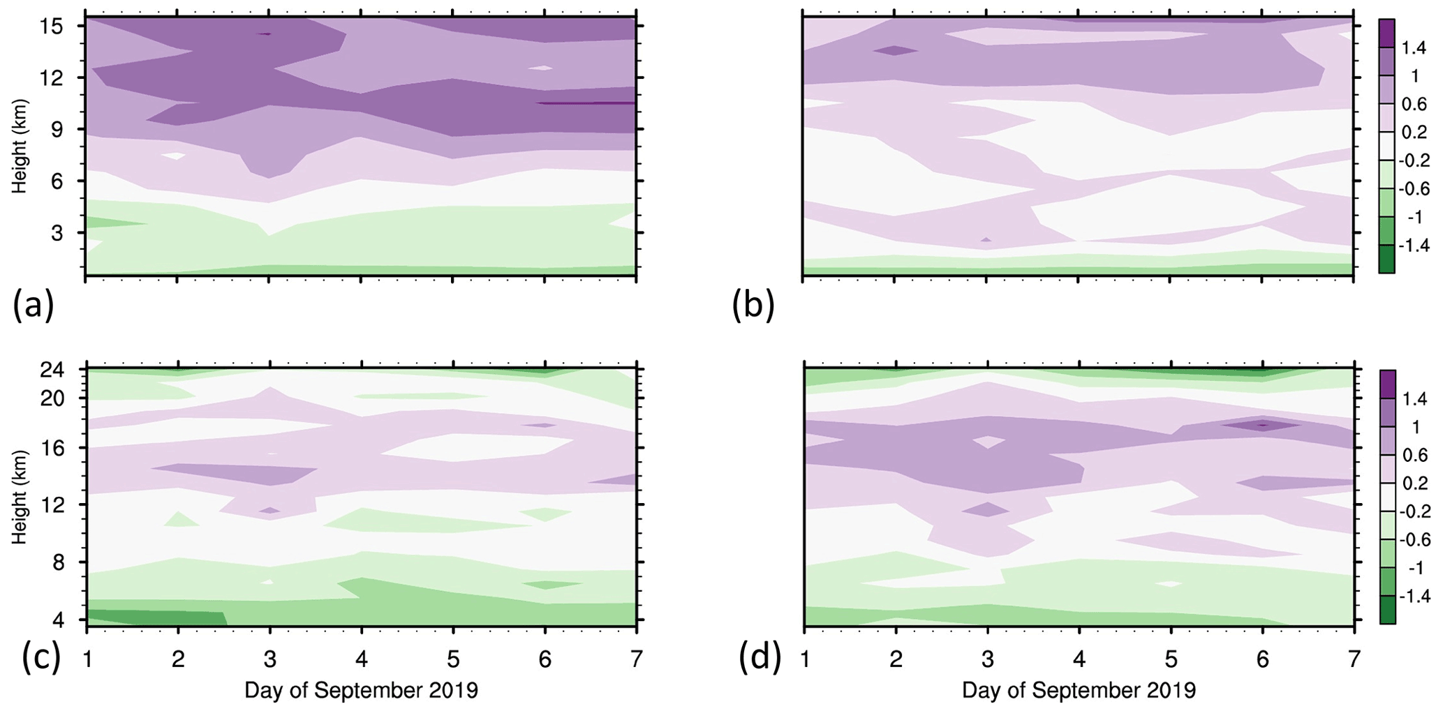
Figure 2 Vertical and daily variations in global horizontal biases (m s⁻¹) for Mie winds (a, b) and Rayleigh winds (c, d) in ascending (a, c) and descending (b, d) orbits.

For clarity in the remainder of this article, certain words and phrases are assigned specific definitions. Thus, throughout this article, the phrase “Aeolus winds” specifically means the observations of Aeolus Level-2B (B10) HLOS winds. Similarly, the phrase “FV3GFS winds” specifically means the numerical weather prediction (NWP) background HLOS winds evaluated from the FV3GFS 6 h forecasts at the observation location and time. (In discussions of winds that are not HLOS winds, terms like u wind, v wind, or wind vector are used.) Further, the phrase “Mie winds” specifically means Aeolus winds derived from Mie backscatter observations, and the phrase “Rayleigh winds” specifically means Aeolus winds derived from Rayleigh backscatter observations. Also, throughout this article, the word “innovations” without further qualification specifically refers to the differences between these Aeolus and FV3GFS winds, and the word “bias” (and the phrases “Mie bias” and “Rayleigh bias”) without further qualification specifically refers to the mean of these innovations, where the sample mean is over some specified space–time volume for either the Mie or Rayleigh winds.

Speed-dependent biases identified and estimated using ordinary least squares (OLS) are subject to contamination from random errors in Aeolus and/or FV3GFS winds (Frost and Thompson, 2000), since OLS assumes no errors in the predictor or independent variable, which in this case would be either the Aeolus or FV3GFS winds or a combination of the two. In contrast, total least squares (TLS) regression accounts for errors in both dependent and independent variables and generates a statistically optimal analysis of the biases (Deming, 1943; Ripley and Thompson, 1987; Markovsky and Van Huffel, 2007). For the case of Aeolus and FV3GFS winds, the use of linear TLS regression (Ripley and Thompson, 1987) finds an optimal estimate of the true (assumed linear) relationship between Aeolus and FV3GFS winds.

In this study, the TLS regression approach is used to estimate biases that depend linearly on wind speed. The suboptimality of OLS bias estimates is demonstrated by comparison to the TLS bias estimates, which are treated as the “truth” in this study. A bias correction based on the TLS bias analysis is proposed to optimize Aeolus wind assimilation by the FV3GFS model and thus improve the impact of Aeolus winds on FV3GFS forecasts. Section 2 describes the Aeolus and FV3GFS winds, the TLS bias analysis method, and the estimation of the ratio of error variances of Aeolus to FV3GFS winds, for which the ratio is used in the TLS regression. Section 3 describes the variations in the TLS bias estimates with height, latitude, and wind speed. Section 4 demonstrates the substantial differences between the TLS and OLS bias estimates. Section 5 proposes a TLS bias correction for Aeolus data assimilation. The forecast impact of the TLS bias correction is presented in Sect. 6. Section 7 presents a summary of the findings and conclusions.

2 Data and methodology

2.1 Aeolus L2B and FV3GFS background wind data

The Aeolus L2B cloudy-sky Mie winds and clear-sky Rayleigh winds are examined for the period 1–7 September 2019. This 1-week period provides a sufficient sample to estimate the biases. The Aeolus winds were obtained from the Aeolus dataset (baseline B10) reprocessed by ESA (Rennie et al., 2021, Weiler et al., 2021). The reprocessing includes the M1 bias correction, which removes most of the globally and vertically averaged biases of both Mie and Rayleigh winds (Weiler et al., 2021). The Aeolus winds are reported at a standard set of vertical layers (de Kloe, 2020). This study examines Mie and Rayleigh winds within height ranges of 0–22 km that include nearly all Aeolus winds. The height is defined relative to the EGM96 geoid for the L2B winds (Tan et al., 2008).

The Aeolus and FV3GFS winds are obtained from a data assimilation experiment (hereafter the BASE experiment), where the Aeolus winds are monitored, and the Aeolus wind observation operator (H_i) is applied to the FV3GFS background (x^b) to obtain the value of FV3GFS wind ($y_i^{\mathrm{b}}=H_i(x^{\mathrm{b}}$)) corresponding to each Aeolus wind $\left(y_i^{\mathrm{o}}\right)$. This experiment employs the FV3GFS data assimilation system, called Global Statistical Interpolation (GSI; Kleist et al., 2009), configured for the 4DEnVar algorithm, with 64 vertical levels and horizontal resolutions of C384 (∼25 km) for the deterministic analysis and forecast and C192 (∼50 km) for the 80 ensemble members (Wang and Lei, 2014).

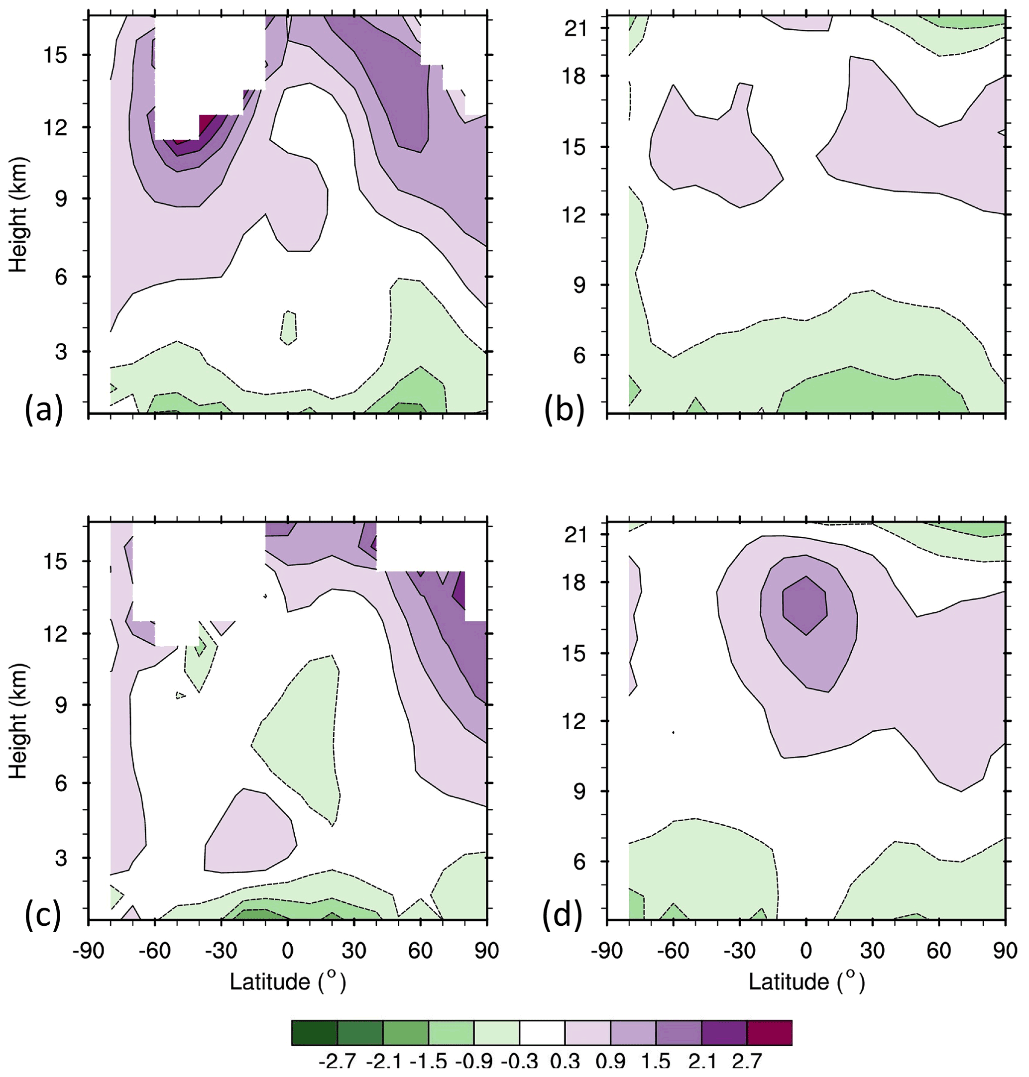
Figure 3 Latitudinal and height distributions of Mie biases (a, c) and Rayleigh biases (b, d) (color scale; m s⁻¹) in ascending (a, b) and descending (c, d) orbits.

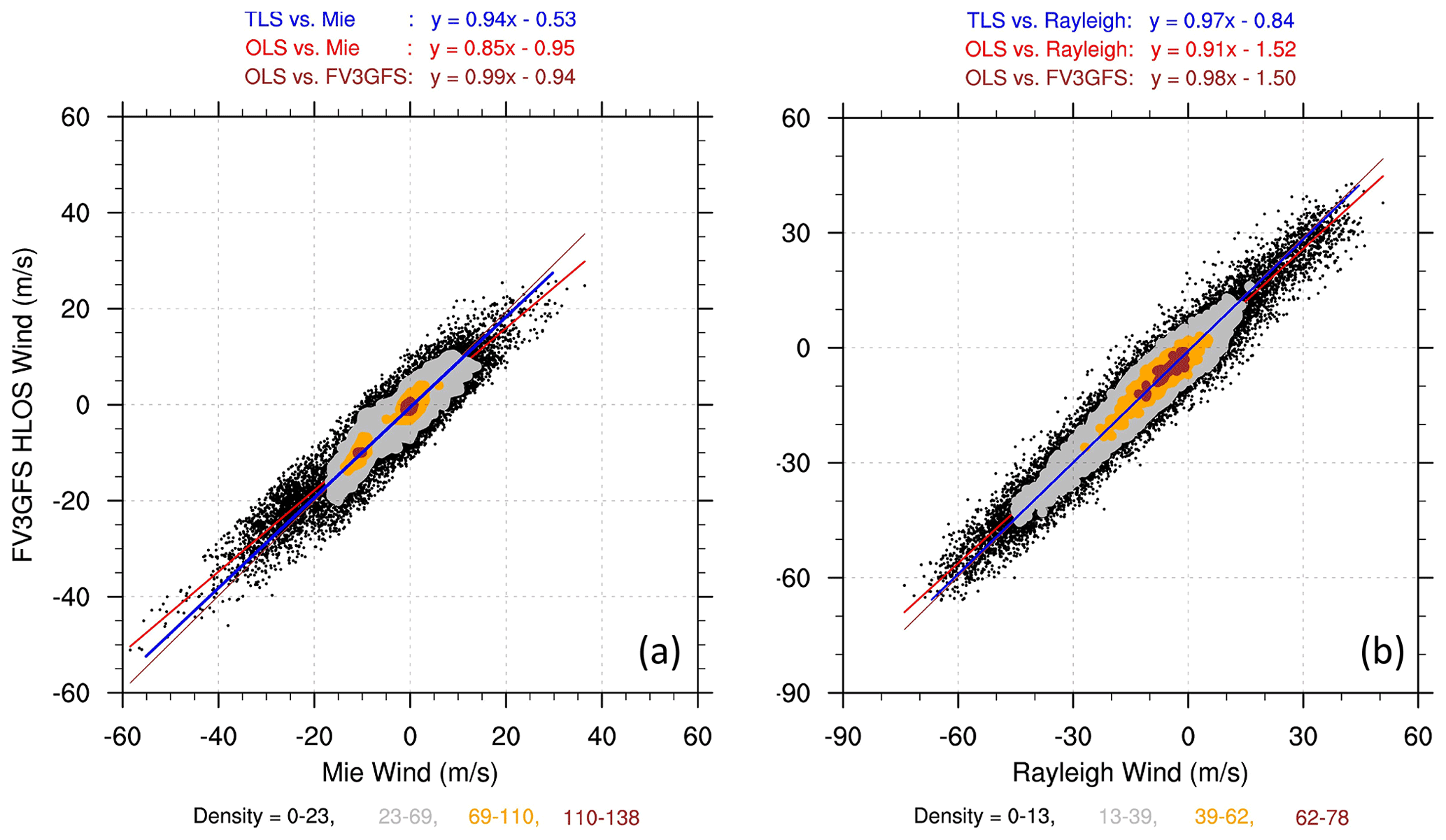
Figure 4 Density plots of global collocated (a) Mie and FV3GFS winds in the layer at ∼3.5 km altitude and (b) Rayleigh and FV3GFS winds in the layer at ∼15 km altitude in descending orbits. The TLS analysis lines (blue), the OLS regression lines of FV3GFS winds on Aeolus winds (red), and the OLS regression lines of Aeolus winds on FV3GFS winds (transformed and plotted as a function of Aeolus winds in brown) are shown, with the corresponding regression coefficients displayed above each panel.

Figure 5 Density plots of global (a) Mie–FV3GFS winds in the layer at ∼3.5 km altitude and (b) Rayleigh–FV3GFS winds in the layer at ∼15 km altitude in descending orbits. The average innovation (brown dots), the OLS regression lines of the innovations on Aeolus winds (brown), and TLS analysis lines (blue) are shown.

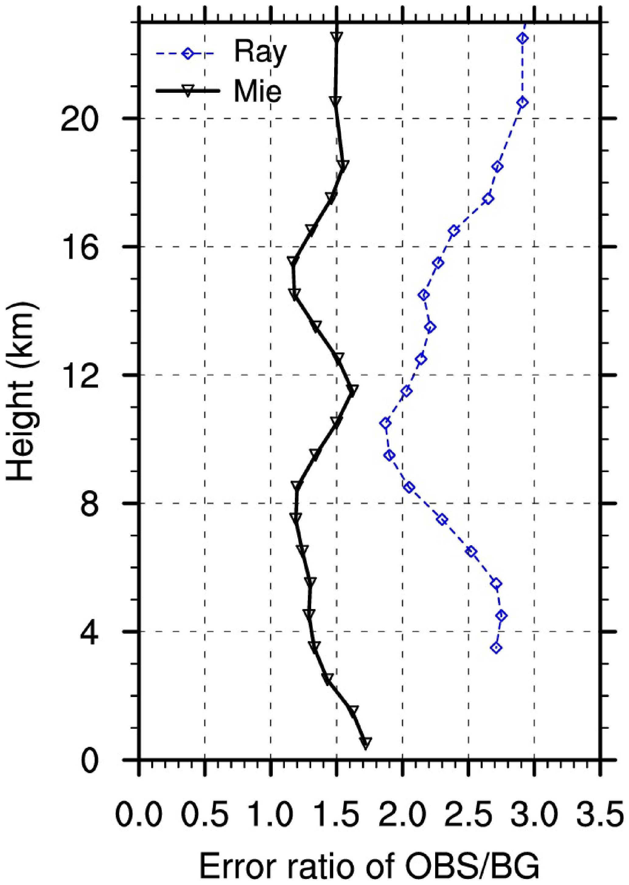
Figure 6 Vertical variation in the square root of the ratio of random error variance in Mie (solid black) and Rayleigh (dashed blue) winds versus FV3GFS winds. Results are based on global innovations from the BASE experiment using the Hollingsworth–Lonnberg method. The symbols are plotted at the average height of the observations in each layer.

Figure 7 Vertical variations in TLS bias coefficients for Mie (a–c), and Rayleigh (d–f) winds. Each point plotted represents a separate TLS analysis for all observations in each layer for all latitudes and for either ascending (black solid) or descending (blue dashed) orbits. The symbols are plotted at the average height of the observations in each layer.

Figure 8 Vertical distributions of average TLS estimated biases (color scale; m s⁻¹) for Mie (a, c) and Rayleigh (b, d) winds as a function of observed Aeolus winds (m s⁻¹) in ascending (a, b) and descending (c, d) orbits for all latitudes. The TLS estimated biases are obtained from the TLS fits displayed in Fig. 7.

Similar Aeolus data quality control procedures, as recommended by ESA and ECMWF (Rennie et al., 2021), were implemented to reject the following observations: the HLOS L2B confidence flag “invalid”, Rayleigh winds at layers below 850 hPa, L2B uncertainties greater than 12 m s⁻¹, accumulation lengths less than 60 km, and atmospheric pressure within 20 hPa of topographic surface pressure, and Mie winds with L2B uncertainties greater than 5 m s⁻¹ and accumulation lengths less than 5 km. Further, a standard outlier check rejects any Aeolus wind for which $|y_i^{\mathrm{o}}-y_i^{\mathrm{b}}|$ is greater than 4 times the estimated errors for Aeolus winds prescribed by the data assimilation system.

When examining Aeolus wind statistics, we stratify the Aeolus data by orbital phase, either ascending when the spacecraft is moving northward or descending when the spacecraft is moving southward. The vertical and daily variations in Mie and Rayleigh biases for global horizontal samples are consistent throughout the period (Fig. 2). For ascending orbits, the Mie biases are positive above 6 km and negative below 6 km and are as large as +1.8 and −0.5 m s⁻¹, respectively. The Mie biases are smaller and positive at most levels in descending orbits. In descending orbits, the Rayleigh biases are as positive as +1.2 m s⁻¹ above 10 km and as negative as −1.2 m s⁻¹ below 8 km. The positive biases in ascending orbits are smaller. The results indicate that the biases vary substantially with height and orbit phase for both Mie and Rayleigh winds. The Mie and Rayleigh biases also vary considerably with latitude (Fig. 3). Mie biases are as positive as +1.5 m s⁻¹ in the upper troposphere, and Rayleigh biases are as positive as +2.0 m s⁻¹ in the tropical upper troposphere. Both Mie and Rayleigh biases are as negative as −1.0 m s⁻¹ in the lowest layers.

The statistical relationship between Aeolus and FV3GFS winds is illustrated by the density plots in Fig. 4. There is a strong correlation of 0.93 between Mie and FV3GFS winds and of 0.96 between Rayleigh and FV3GFS winds. The average and OLS regression of the innovations as a function of Aeolus wind suggest considerable speed-dependent biases with both linear and nonlinear components (Fig. 5). In this study, we focus on the estimation and correction of the linear part of the biases using the TLS linear regression.

2.2 TLS linear regression

In this section, we review the TLS linear regression method (Ripley and Thompson, 1987) in the context of estimating potential speed-dependent biases. The TLS estimate for each collocated pair of Aeolus and FV3GFS winds ($y_i^{\mathrm{o}}$, $y_i^{\mathrm{b}})$ is defined by the following:

$$\begin{array}{}\text{(1)}& y_i^{\mathrm{o}}={\widehat{y}}_i^{\mathrm{o}}+{\mathit{\epsilon }}_i^{\mathrm{o}}\mathrm{and}{y}_i^{\mathrm{b}}={\widehat{y}}_i^{\mathrm{b}}+{\mathit{\epsilon }}_i^{\mathrm{b}}(i=\mathrm{1},N),\end{array}$$

where ${\widehat{y}}_i^{\mathrm{o}}$ and ${\widehat{y}}_i^{\mathrm{b}}$ are the TLS estimates of the true Aeolus and FV3GFS winds, ${\mathit{\epsilon }}_i^{\mathrm{o}}$ and ${\mathit{\epsilon }}_i^{\mathrm{b}}$ are random errors, and N is the number of Aeolus/FV3GFS wind collocations in the sample. The sample might be defined by a vertical layer or a latitude band. In OLS regression, since it is assumed that there are no errors in the predictor, the predictor can be used directly to estimate the predictand. The situation is a little more complicated in TLS regression, where (${\widehat{y}}_i^{\mathrm{b}}$, ${\widehat{y}}_i^{\mathrm{o}})$, the most probable true state, is the point on the regression line that is closest in a statistical sense to the point $(y_i^{\mathrm{b}}$, $y_i^{\mathrm{o}})$.

Here it is assumed that ${\mathit{\epsilon }}_i^{\mathrm{o}}$ and ${\mathit{\epsilon }}_i^{\mathrm{b}}$ are independent and that the random error variance ratio $\mathit{\delta }=\left({\mathit{\sigma }}^{\mathrm{o}}/{\mathit{\sigma }}^{\mathrm{b}}\right){}^{\mathrm{2}}=E\left[{\mathit{\epsilon }}_i^{\mathrm{o}}{\mathit{\epsilon }}_i^{\mathrm{o}}\right]/E\left[{\mathit{\epsilon }}_i^{\mathrm{b}}{\mathit{\epsilon }}_i^{\mathrm{b}}\right]$ is known. The error variance ratio δ is a crucial parameter in determining the TLS bias analysis and is estimated as described in the next section. Furthermore, the true relationship between the Aeolus and FV3GFS winds is assumed to be described by a linear function (as seen in Fig. 5) as follows:

$$\begin{array}{}\text{(2)}& {\widehat{y}}_i^{\mathrm{o}}=c_{\mathrm{0}}+c_{\mathrm{1}}{\widehat{y}}_i^{\mathrm{b}}(i=\mathrm{1},N),\end{array}$$

where c₀ is an offset or constant coefficient, and c₁ is a speed-dependent coefficient.

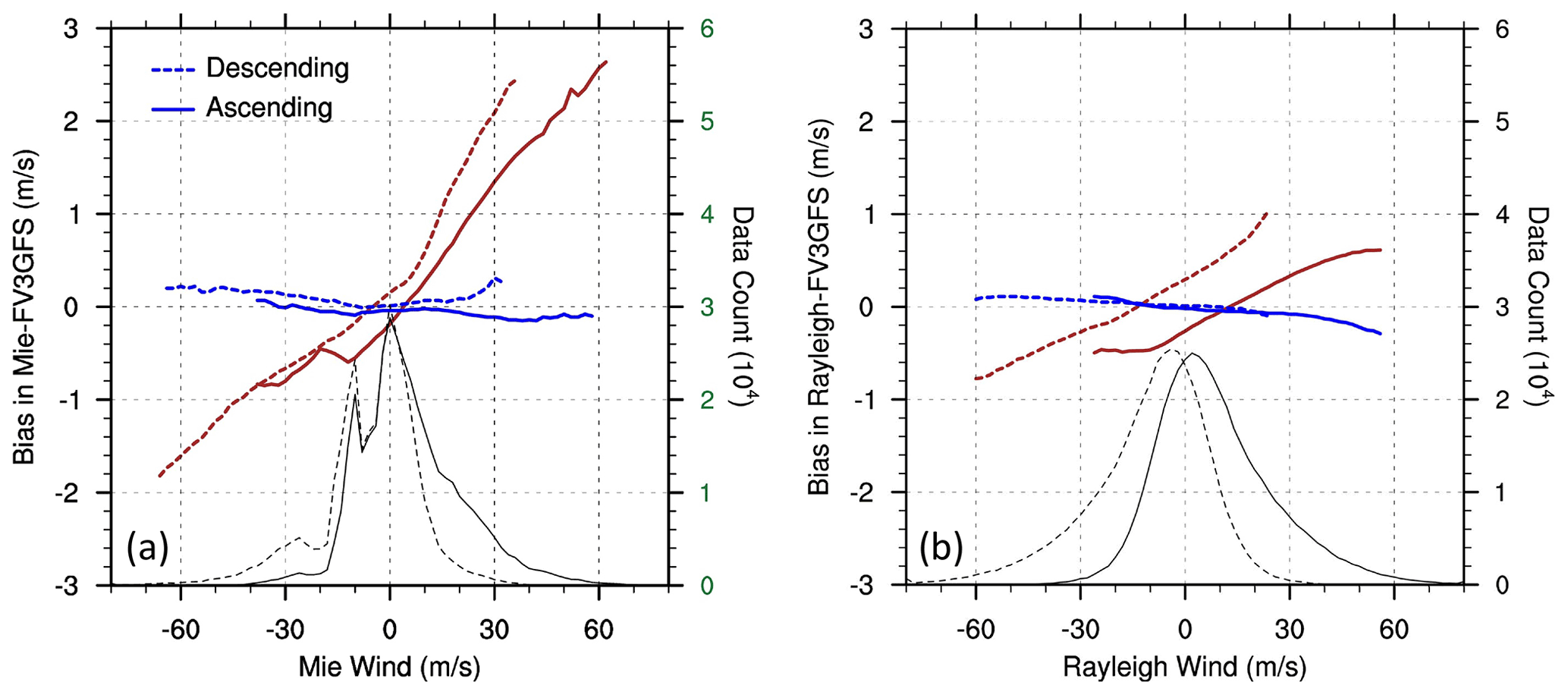
Figure 9 TLS estimated biases (m s⁻¹) before (brown lines) and after (blue lines) TLS bias correction for Mie (a) and Rayleigh (b) winds as a function of the observed Aeolus winds (m s⁻¹), vertically averaged for all latitudes of Aeolus winds. The solid and dashed lines are for ascending and descending orbits, respectively. The black lines report the number of Aeolus winds in each 2 m s⁻¹ bin.

The TLS regression finds an optimal estimate of the ${\widehat{y}}_i^{\mathrm{b}}$, c₀, and c₁ by minimizing the cost function J, as follows:

$$\begin{array}{}\text{(3)}& \begin{array}{rl}J& ={\sum }_{i=\mathrm{1}}^N\left({\left({\mathit{\epsilon }}_i^{\mathrm{o}}/{\mathit{\sigma }}^{\mathrm{o}}\right)}^{\mathrm{2}}+{\left({\mathit{\epsilon }}_i^{\mathrm{b}}/{\mathit{\sigma }}^{\mathrm{b}}\right)}^{\mathrm{2}}\right)\\ & ={\displaystyle \frac{\mathrm{1}}{{\left({\mathit{\sigma }}^{\mathrm{o}}\right)}^{\mathrm{2}}}}{\sum }_{i=\mathrm{1}}^N\left({\left(y_i^{\mathrm{o}}-c_{\mathrm{0}}-c_{\mathrm{1}}{\widehat{y}}_i^{\mathrm{b}}\right)}^{\mathrm{2}}\right.\\ & \left.+\mathit{\delta }{\left(y_i^{\mathrm{b}}-{\widehat{y}}_i^{\mathrm{b}}\right)}^{\mathrm{2}}\right).\end{array}\end{array}$$

To determine the ${\widehat{y}}_i^{\mathrm{b}}$, the derivative of J with respect to ${\widehat{y}}_i^{\mathrm{b}}$ is set to zero, resulting in the following:

$$\begin{array}{}\text{(4)}& {\widehat{y}}_i^{\mathrm{b}}=\left(c_{\mathrm{1}}\left(y_i^{\mathrm{o}}-c_{\mathrm{0}}\right)+\mathit{\delta }{y}_i^{\mathrm{b}}\right)/\left(c_{\mathrm{1}}^{\mathrm{2}}+\mathit{\delta }\right)(i=\mathrm{1},N).\end{array}$$

Equation (4) thereby reduces the problem to a minimization in terms of c₀ and c₁. A similar equation holds even if the error variances vary with i, but then there is no closed form solution for c₀ and c₁ as there is in the current case, which is known as the Deming problem (Ripley and Thompson, 1987). When the coefficients c₀ and c₁ are obtained, the TLS estimate for the new or within-sample observation is given by Eq. (4). Finally, the estimate of the bias for the kth observation, either for a new or within-sample observation, is given by the following:

$$\begin{array}{}\text{(5)}& {\widehat{d}}_k={\widehat{y}}_k^{\mathrm{o}}-{\widehat{y}}_k^{\mathrm{b}}=c_{\mathrm{0}}+(c_{\mathrm{1}}-\mathrm{1}){\widehat{y}}_k^{\mathrm{b}}.\end{array}$$

Given the form of Eq. (5), we will refer to c₀ and (c₁−1) as the offset and speed-dependent bias coefficients, respectively, hereafter.

2.3 Estimation of the random error variance ratio

In this study, errors of Aeolus winds are estimated by the Hollingsworth–Lonnberg method (Hollingsworth and Lonnberg, 1986; Garrett et al., 2022), which include Aeolus instrument errors and forward modeling error and representativeness errors of the FV3GFS background at the specific 25 km horizontal resolution. The random error variance ratio $\mathit{\delta }=({\mathit{\sigma }}^{\mathrm{o}}/{\mathit{\sigma }}^{\mathrm{b}}{)}^{\mathrm{2}}$ in the TLS bias analysis is estimated from the innovations from the BASE experiment for 1–7 September 2019. It is assumed that there are no correlations between the random errors of the Aeolus and FV3GFS winds and no horizontal correlations between the random errors of Aeolus winds separated by more than 90 km. These assumptions are justified a posteriori by the reasonable error estimate of FV3GFS background winds (Garrett et al., 2022).

Global error estimates are calculated for all Mie and Rayleigh winds in each layer as follows. First, the spatial covariance of the innovations is calculated. Since these are innovations from the BASE experiment where Aeolus data are not assimilated, it is reasonable to assume that the Aeolus and FV3GFS wind errors are uncorrelated. Then the spatial covariance of the innovations, (σ^o−b)², at zero separation distance, is equal to the following:

$$\begin{array}{}\text{(6)}& ({\mathit{\sigma }}^{\mathrm{o}-\mathrm{b}}{)}^{\mathrm{2}}=({\mathit{\sigma }}^{\mathrm{o}}{)}^{\mathrm{2}}+({\mathit{\sigma }}^{\mathrm{b}}{)}^{\mathrm{2}},\end{array}$$

where σ^o and σ^b are the random error standard deviations of Aeolus and FV3GFS winds, respectively.

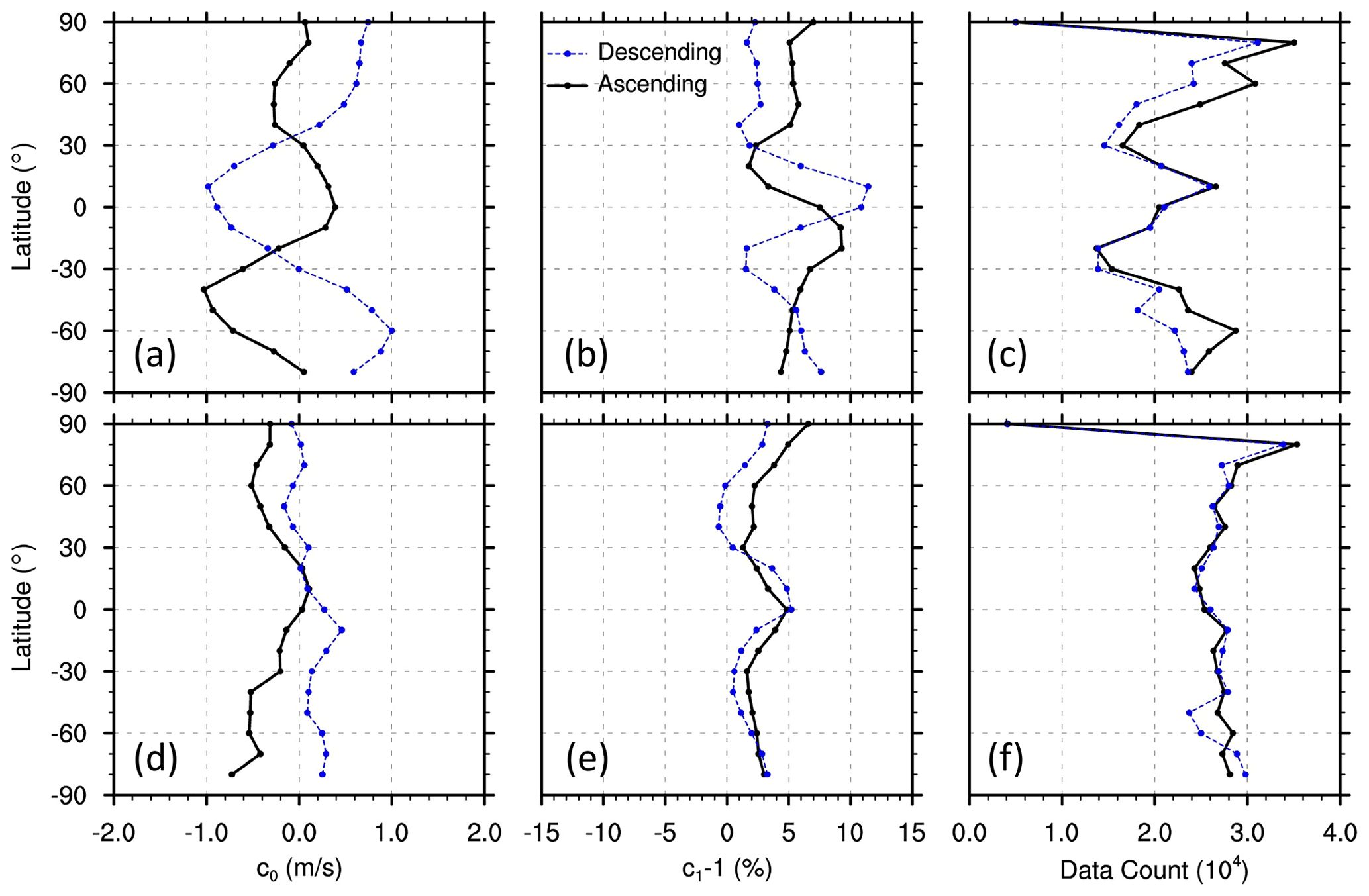
Figure 10 Latitudinal variation in TLS bias coefficients for Mie (a–c) and Rayleigh (d–f) winds. Each point plotted represents a separate TLS analysis for all observations in all vertical layers in a 10^∘ latitude band for either ascending (black solid) or descending (blue dashed) orbits. The latitude bands are centered every 10^∘ from 90^∘ S to 90^∘ N. The symbols are plotted at the center in each latitude band. The vertical layers are 0–16 km for Mie winds and 3–22 km for Rayleigh winds.

By assumption, at separation distances greater than 90 km, the innovation covariances are estimates of the FV3GFS wind error covariance alone and can be extrapolated back to zero separation to obtain an estimate of the error variance of the FV3GFS winds, (σ^b)², and then, using Eq. (6), the error variance of the Aeolus winds, (σ^o)², may be determined. Note that this can only be done using innovation covariances at separation distances large enough to have negligible covariances between the Aeolus winds. Since the calculated innovation covariances are globally averaged over all HLOS winds, it is not surprising that the corresponding biases are small. The small residual biases in the innovations may introduce small (<0.1) spurious spatial correlations. This spurious correlation, taken as the value calculated for the last bin (at 990 km), is removed from the correlation curves at all separation distances. The estimated random error variance ratio δ is assigned to the layer center height, defined as the global average heights of the Mie and Rayleigh wind in each vertical range bin. Figure 6 shows that the vertical profiles of the square root of δ vary in the range of 1.2–1.6 for Mie winds versus FV3GFS winds and 2–3 for Rayleigh winds versus FV3GFS winds, respectively.

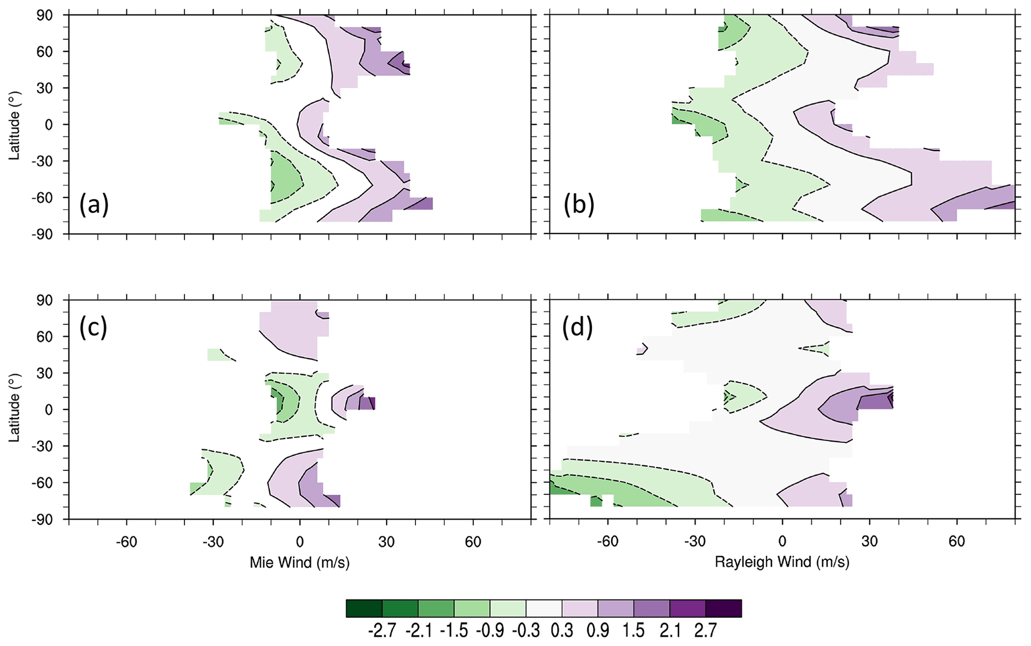
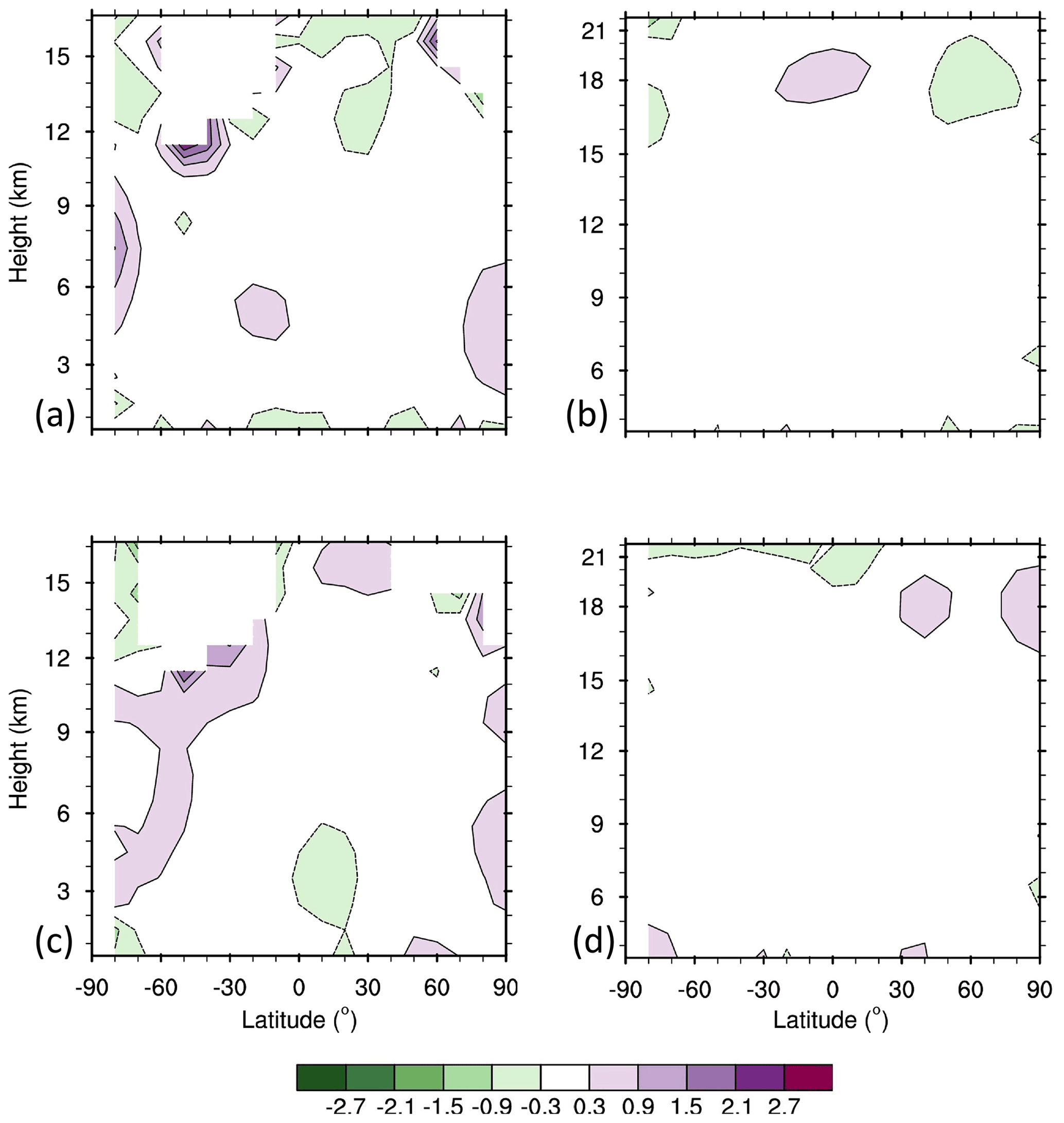
Figure 11 Latitudinal distributions of average TLS estimated biases (color scale; m s⁻¹) for Mie (a, c) and Rayleigh (b, d) winds as a function of Aeolus wind in ascending (a, b) and descending (c, d) orbits, obtained from the TLS fits displayed in Fig. 10.

Figure 12 Vertical distributions of average bias estimates (color scale; m s⁻¹) for Mie (a, c, e) and Rayleigh (b, d, f) winds as a function of Aeolus winds using one of three methods for descending orbits for all latitudes. The methods are OLS using FV3GFS winds as a predictor (a, b), TLS (c, d; same as the bottom panels of Fig. 8), and OLS using the average of Aeolus and FV3GFS as a predictor (e, f).

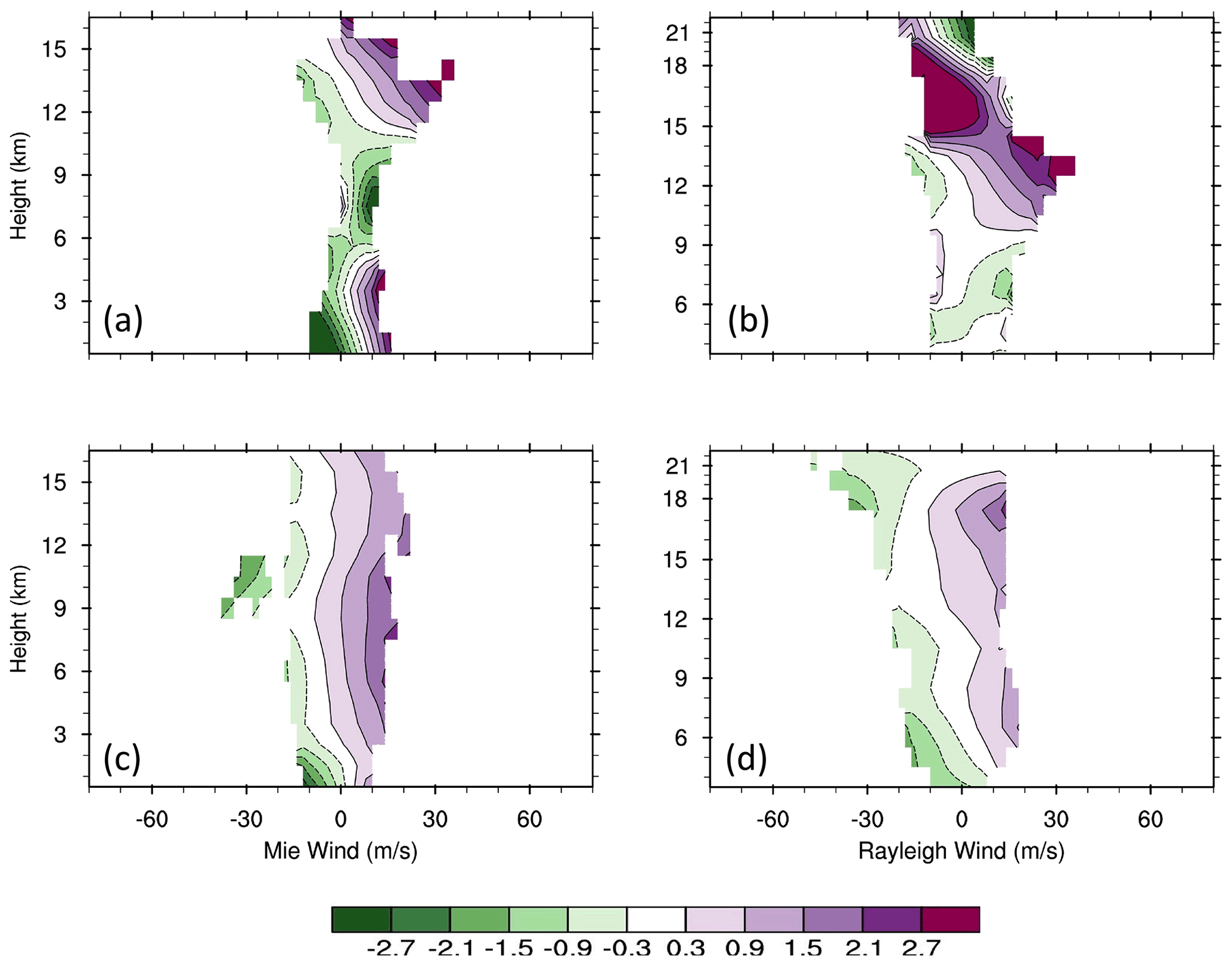
Figure 13 Vertical distributions of average TLS estimated biases (color scale; m s⁻¹) for Mie (a, c) and Rayleigh (b, d) winds as a function of Aeolus winds (m s⁻¹) in the latitudinal bands centered at the Equator (a, b) and at 80 S (c, d) for the descending orbits.

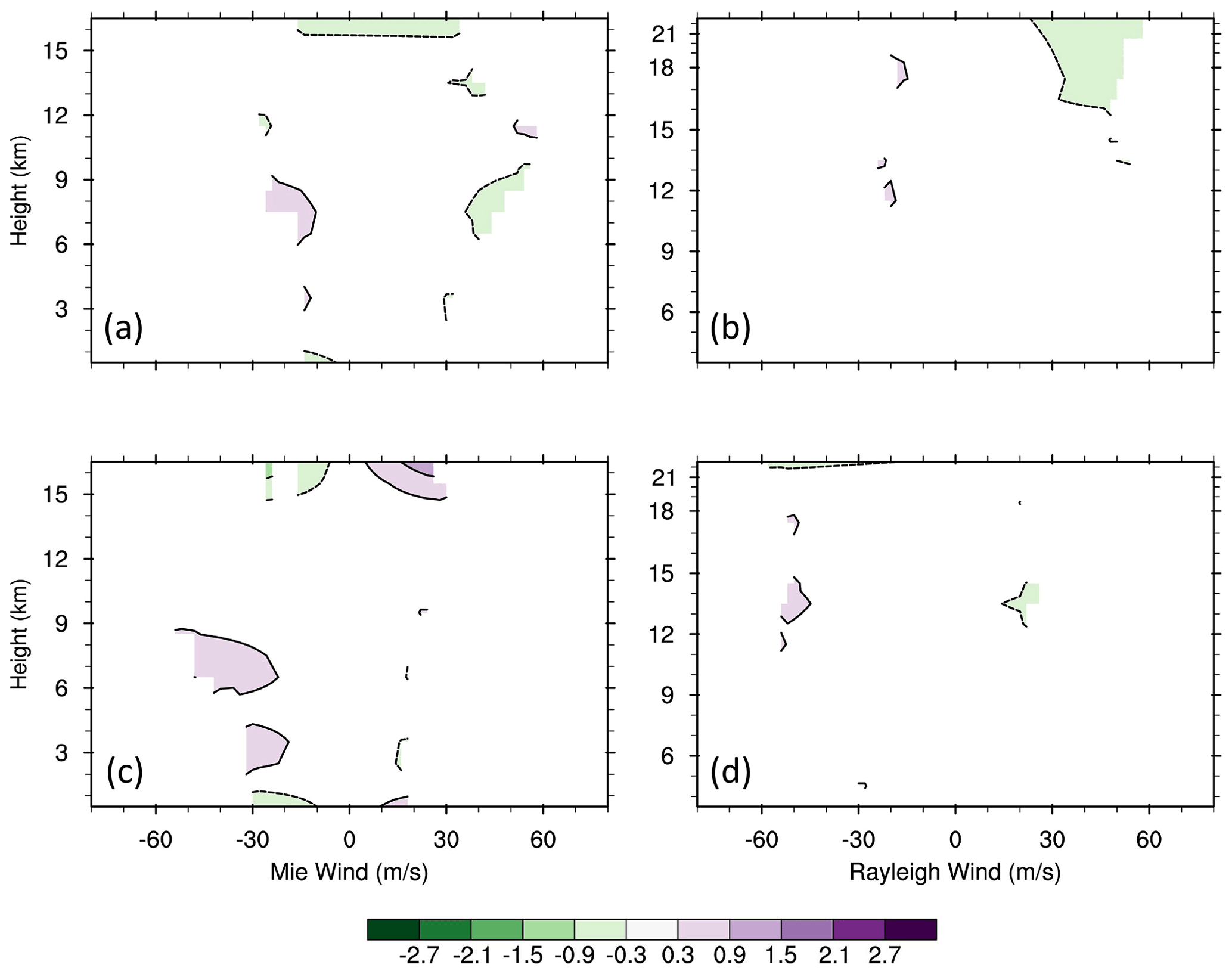
Figure 14 As in Fig. 8 but for the mean innovation after the TLS bias correction is applied. For each 6 h cycle during 1–7 September 2019, the TLS bias correction is calculated from the 28 preceding 6 h cycles.

Figure 15 As in Fig. 3 but after the TLS bias correction is applied.

In the future, we plan to explore the benefit of the scene-dependent L2B estimated errors on the TLS bias estimates and Aeolus wind assimilation.

3 The TLS bias estimates

In this section, variations in the TLS bias estimates with orbital phase and height are examined to motivate the use of a TLS bias correction scheme proposed in Sect. 5.

3.1 Variation in TLS bias estimates with height

The variation in the TLS solution with height and orbital phase is described here. The TLS samples include winds at all latitudes in each layer. The vertical distribution of the TLS constant and speed-dependent bias analysis coefficients in Eq. (5) is shown in Fig. 7. The speed-dependent bias coefficient (c₁−1) varies substantially with height and orbital phase. For Mie winds, this coefficient is quite large at most heights, ranging from 3 % to 6 %, with maxima at 3 and 12–16 km. For Rayleigh winds, this coefficient is smaller and ranges from 1 % to 3 % in ascending orbits and 1 %–5 % in descending orbits, with maxima around 3.5 and 16 km.

The offset bias coefficient c₀ for both Mie and Rayleigh winds also shows large variations with height and orbit, with its value as large as ±1.0 m s⁻¹. In general, the offset bias coefficient is positive in upper layers and negative in layers close to the Earth's surface, consistent with the patterns seen in the global horizontal average of the innovations in Fig. 2. The vertical distribution of the average TLS bias estimate as a function of Aeolus wind is shown in Fig. 8. The biases vary substantially with height. Since the TLS biases are in part dependent on speed, at most heights the biases increase substantially as the magnitude of Aeolus wind speed increases. The biases at the extreme Aeolus wind speeds are as large as +2.5 and −1.0 m s⁻¹ for Mie winds and +1.5 and −1.0 m s⁻¹ for Rayleigh winds. There are clear speed-dependent biases in the vertical average of these biases as well (Fig. 9). The results suggest that the innovations have both vertically varying and vertically averaged speed-dependent biases.

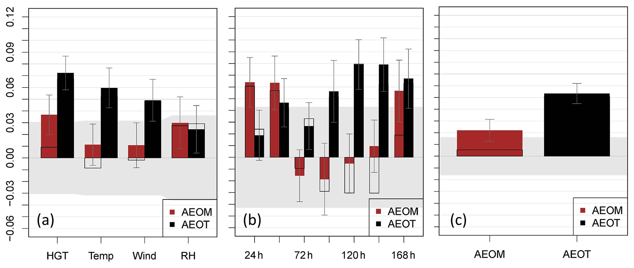
Figure 16 The summary assessment metric (SAM) overall forecast scores for AEOM and AEOT versus BASE experiments in the North American (NA) region for day 1–7 forecasts validated at 00:00 UTC 22–28 November 2019. The scores are shown for (a) forecast parameters of temperature (Temp), geopotential height (HGT), vector wind (Wind), relative humidity (RH), (b) lead times, and (c) the overall performance of AEOM and AEOT. The forecasts are verified to their self-analyses. Values above 0.0 demonstrate an increase in the mean of the normalized distribution and improvement of the forecast versus the BASE, while the shaded region represents the 95 % significance level. The gray areas indicate the 95 % confidence level under the null hypothesis that there is no difference between experiments for this metric. In addition, the estimated uncertainty at the 95 % level is indicated by small error bars at the ends of the color bars. In total, two normalizations are used, i.e., the ECDF (colors) and rescaled min/max normalization (black outline). Details can be found in Hoffman et al. (2018). A value of 0.02, for example, indicates the average normalized statistic over all statistics is better (greater) by 0.02 than BASE. Under the null hypothesis that there are no differences, all SAMs would be one-half, so a 0.02 improvement can be considered a 4 % improvement ($\mathrm{0.02}/\mathrm{0.5}$) in normalized scores.

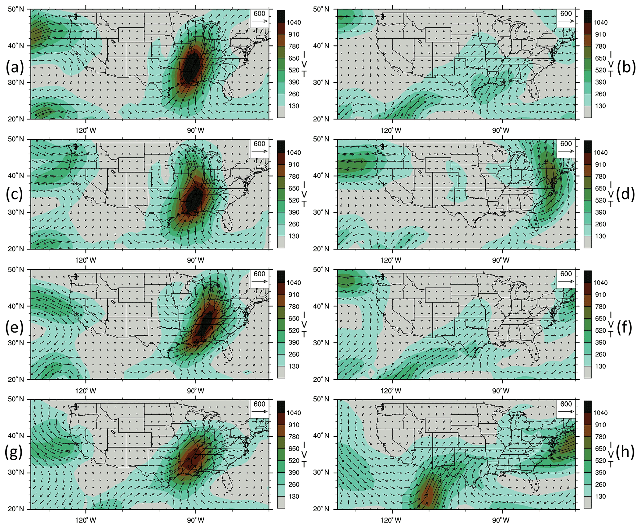
Figure 17 The 200–1000 hPa vertically integrated water vapor transport (IVT; kg m s⁻¹; contour) and wind vectors (m s⁻¹; arrows) in the day 7 forecasts, validated at 00:00 UTC on 27 (a, c, e) and on 28 (b, d, f) November 2019 for (a, b) BASE, (c, d) AEOM, (e, f) AEOT, and (g, h) ECMWF analyses.

3.2 Variation in biases with latitude

The variation in the TLS solution with latitude and orbital phase is described here. For this purpose, the samples include all heights in each 10^∘ latitude band, and the vertical average of the error ratio δ is used. In general, the bias coefficients obtained are large and vary considerably with latitude and orbital phase, with maxima found in the tropics (Fig. 10). For example, the speed-dependent bias coefficient (c₁−1) for Mie winds in the tropics can be quite large, ranging up to a maximum of 11 %. This coefficient is smaller for Rayleigh winds, ranging from −1 % to 5 %, with maxima found in the tropics. The offset bias coefficient c₀ for Mie winds also varies considerably with latitude and orbit, ranging from −1.0 to +1.6 m s⁻¹. The offset bias coefficient c₀ is smaller for Rayleigh winds.

The latitudinal distribution of the average TLS bias as a function of Aeolus wind speed is shown in Fig. 11. For both Mie and Rayleigh winds, the average TLS biases increase considerably at most latitudes as the magnitude of Aeolus wind speed increases, particularly in the tropics and SH, with extreme values of about ±1.5 m s⁻¹.

3.3 Discussion

The results indicate that the speed-dependent bias coefficient (c₁−1) is quite large, reaching ∼10 % and 5 % for Mie and Rayleigh winds, respectively, particularly in the lower stratosphere and lower troposphere of the tropics. This suggests that there exist large speed-dependent biases in the FV3GFS and/or Aeolus winds. Given that there exist large uncertainties in the FV3GFS (and ECMWF) background winds in the tropics (see Fig. 1), it is likely that the FV3GFS background may be a significant source of the biases, and this will require further investigation. In any case, these large speed-dependent biases should be corrected to optimize Aeolus wind assimilation and the impact of Aeolus winds on NWP forecasts. The large variations in the TLS bias estimates with latitude and height guide the design of the proposed TLS bias correction in Sect. 5.

4 Comparison to OLS regressions

Parallel OLS regressions using three different predictors of the biases are compared with the TLS bias estimate results presented in Sect. 3. The OLS predictors are the FV3GFS winds, the Aeolus winds, and their average. The first two of these OLS regressions are equivalent to OLS regressing Aeolus winds on FV3GFS winds and OLS regressing FV3GFS winds on Aeolus winds. The regression lines of these two cases are added to Fig. 4. The TLS speed-dependent coefficient (c₁−1) (in Eq. 5) is 6 % and 4 % for Mie and Rayleigh winds, respectively. However, the OLS regression of Aeolus winds on FV3GFS winds produces considerably smaller bias estimates, with (c₁−1) estimated as 1 % and 2 % for Mie and Rayleigh winds, respectively. On the other hand, the OLS regression of the FV3GFS winds on Aeolus winds exhibits much larger bias estimates relative to the TLS bias analysis, with (c₁−1) estimated as 18 % and 15 % for Mie and Rayleigh winds, respectively.

The vertical distributions of the average biases as a function of Aeolus winds are shown in Fig. 12 for the descending orbits for the following three methods: (1) OLS regression using FV3GFS winds as a predictor (top row), (2) TLS regression (middle row, which repeats the bottom two panels of Fig. 8), and (3) OLS regression using the average of FV3GFS and Aeolus as a predictor (bottom row). The average bias estimates in the top panels are about 0.5 m s⁻¹ smaller in magnitude in most layers compared to the middle panels. The average biases in the bottom panels are about 0.5–1.0 m s⁻¹ in magnitude larger than the middle panels in most layers, particularly for Rayleigh winds. The bias estimates of OLS regression using Aeolus winds only as a predictor (not shown) are even larger than what is shown in the bottom panels. The large differences in the bias estimates using the TLS and OLS regression are due to the fact that both Aeolus and FV3GFS winds have large errors. If the predictor (either Aeolus or FV3GFS winds) has very small errors, then the OLS regressions would be close to perfect, and the OLS and TLS regressions would give very similar results. In such situation, the random error ratio would be either infinity small (≪1) or infinity large (≫1). However, the Aeolus and FV3GFS winds have considerable errors, and the actual random error ratio is about 2–3 for the Rayleigh winds versus FV3GFS winds and about 1.2–1.5 for the Mie winds versus FV3GFS winds (Fig. 6). This leads to the large differences in the OLS and TLS bias estimates. Specifically, the OLS bias estimates using Aeolus winds as a predictor have larger differences from the TLS estimates than the OLS estimates using FV3GFS winds as a predictor.

5 A TLS bias correction

In this section, a TLS bias correction is proposed to optimize Aeolus wind data assimilation. Because the findings in Sect. 3 show substantial variation in the bias coefficients with latitude, vertical layer, and orbital phase, the TLS bias coefficients are calculated from the winds in 19 discrete bins of latitude (centered every 10^∘ between 90^∘ S to 90^∘ N) for each vertical range/layer and for ascending and descending orbits separately. The error ratio δ shown in Fig. 6 is used in all latitude bands for each layer. For each assimilation cycle, the bias coefficients are computed by TLS regression for the innovations in the week before the cycle (i.e., for the previous 28 cycles). The period of 1 week provides a large enough sample for the regression. As shown by Ripley and Thompson (1987), the TLS solution only involves solving a quadratic equation with coefficients given by sample sums. Therefore, an efficient approach is to calculate and save these sums for every cycle and accumulate them over the 28 cycles. For each of the innovations in the assimilation cycle, values of the TLS regression coefficients c₀ and c₁ are linearly interpolated to the latitude of the Aeolus observation. Subsequently, the TLS estimated bias, calculated using Eq. (5), is subtracted from the innovation. Note that the bias correction is determined by the TLS analysis solution for ${\widehat{y}}_k^{\mathrm{b}}$ that, in turn, is determined from the observation and background wind, $y_k^{\mathrm{o}}$ and $y_k^{\mathrm{b}}$, following Eq. (4).

The proposed scheme is applied to the Aeolus and FV3GFS winds of the BASE experiment. As expected, the corresponding TLS bias estimates show considerable speed-dependent biases. For example, in the bins centered at the Equator and 80^∘ S, where the speed-dependent biases are expected to be largest based on Fig. 9, the TLS bias estimates vary considerably with speed and are in some cases larger in magnitude than 1.5 m s⁻¹ at higher Aeolus wind magnitudes (Fig. 13).

The vertical distribution of the global average of the remaining biases (i.e., after TLS bias correction) as a function of Aeolus wind is shown in Fig. 14, which is in the same format and for the same sample of observations as Fig. 8. A comparison of these two figures reveals that most of the biases are removed by the proposed TLS bias correction. The latitudinal variations in the biases are also corrected (Fig. 15). In addition, the biases in the vertical average are also mostly removed, as shown in Fig. 9.

6 Impact of the TLS bias correction on forecast skill

Several observing system experiments (OSEs) using the NOAA global data assimilation system are performed using the Aeolus winds with and without the TLS bias correction. For the period of 2 August–16 September 2019, Garrett et al. (2022) demonstrate the positive impact of Aeolus winds on the NOAA global forecast. The largest impact is seen in the tropical upper troposphere and lower stratosphere where the day 1–3 wind vector forecast root mean square error (RMSE) is reduced by up to 4 %. Specifically, the assimilation of Aeolus impacts the steering currents ambient to tropical cyclones, resulting in up to a 20 % reduction in track forecast error in the eastern Pacific and Atlantic basins. The application of TLS bias correction increases the positive impact of Aeolus data assimilation on the forecasts.

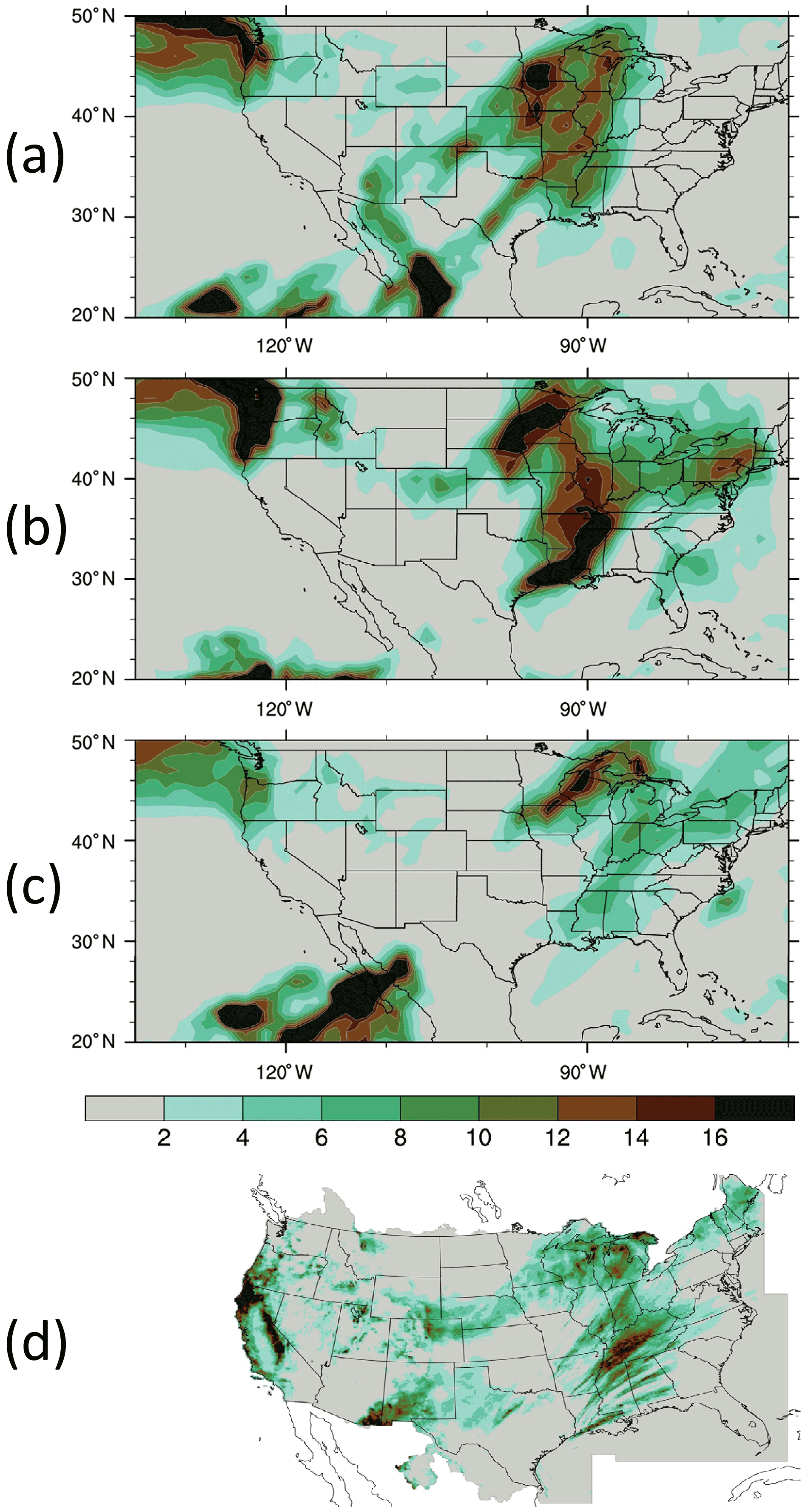
Figure 18 The 24 h accumulated precipitation (mm) for 156 to 180 h, averaged for the forecasts validated from 12:00 UTC 26 to 28 November 2019 for (a) BASE, (b) AEOM, (c) AEOT, and (d) the National Centers for Environmental Prediction (NCEP) precipitation rain gauge data analysis.

Figure 19 The forecast skill scores for 24 h accumulated precipitation for 156 to 180 h forecasts validated from 12:00 UTC on 26–28 November 2019. The equitable threat (a) and bias score (b) are measures of the forecast skill for location and amount of precipitation, respectively. The differences relative to the BASE and the statistical significances are shown in panels (c) and (d), respectively. The equitable threat and bias scores closer to 1.0 indicate improved precipitation forecast skill.

OSE results for a 2019 record-breaking winter storm case over the USA are reported here. On 26 November 2019, one major storm approached the West Coast of the USA from the eastern Pacific and produced a record-breaking low pressure of 973 hPa and wind gust of 171 km h⁻¹ near the Oregon/California border. Over the next few days, the low merged with the subtropical jet as it tracked eastward across the USA. The combination of cold air, moisture, and high winds produced snow blizzard conditions across the USA.

As in Garrett et al. (2022), the OSEs include the baseline experiment (BASE) without the assimilation of Aeolus winds, the experiment AEOM that is identical to BASE except that Aeolus winds are assimilated, and the experiment AEOT hat is identical to AEOM, except that it also includes the TLS bias correction. A difference summary assessment metric (SAM; Hoffman et al., 2018) is computed for day 1–7 forecasts in the North American (NA) region of the experiments validated at 00:00 UTC on 22–28 November 2019. The SAM illustrates the overall forecast skill by normalizing the AC and RMSE values for each parameter (temperature, geopotential height, wind, and relative humidity) and each lead time. Figure 16 shows that the TLS bias correction improves the impact of Aeolus winds on the forecasts of wind, temperature, and geopotential height for day 3–7 and especially for day 5–7 lead times. The overall improvement of Aeolus winds for AEOM and AEOT is about 4 % and 10 %, respectively (above the 95 % significance level, Fig. 16c), illustrating the usefulness of the TLS bias correction.

The vertically integrated water vapor transport (IVT) is a useful metric in forecasting precipitation associated with winter storms (e.g., Lavers et al., 2017). The IVTs of the day 7 forecast for the experiments validated for 00:00 UTC on 27 and 28 November are shown in Fig. 17. Aeolus winds have a strong impact on the locations and intensities of the IVT maxima near the USA West Coast and in the Midwest. In general, the IVTs are closer to the ECMWF analyses in AEOT than in AEOM. As a result, Aeolus winds show strong impact on the locations and corresponding amounts of precipitation, as seen in Fig. 18 and quantified by the equitable threat and BIAS skill scores (https://www.wpc.ncep.noaa.gov/rgnscr/verify.html, last access: 15 January 2022, Wang, 2014), respectively (Fig. 19). Specifically, the precipitation amounts near the West Coast and the Midwest are much less in AEOT than in BASE and AEOM. The precipitation in the Midwest also shifts eastward in AEOT, compared to BASE and AEOM (Fig. 18). The precipitation forecast skills (verified against NCEP precipitation rain gauge data analyses) over the contiguous United States (CONUS) region, that is, the equitable threat (location) and BIAS (amount) scores are shown in Fig. 19. The precipitation amount is overpredicted (BIAS score >1.0) in both BASE and AEOM but is closer to the analysis (BIAS score closer to 1.0) in AEOT. The equitable threat is larger (with marginal significance level; Fig. 19c) in AEOT than in BASE and AEOM, indicating that the location of precipitation in the forecast is improved in AEOT. These results suggest the potential benefit of the TLS bias correction to precipitation forecasts.

7 Summary and conclusions

In this study, a TLS linear regression is used to optimally estimate speed-dependent linear biases in the Aeolus innovations. The Aeolus and FV3GFS winds for 1–7 September 2019 are analyzed. Clear speed-dependent linear biases for both Mie and Rayleigh winds are found, particularly in the lower troposphere and stratosphere of the tropics and Southern Hemisphere. The largest biases are about 10 % and 5 % of FV3GFS wind speed and are as large as ±2.5 and ±1.5 m s⁻¹ at high Aeolus wind magnitudes for Mie and Rayleigh winds, respectively.

It is found that the TLS linear bias estimates are considerably larger than the OLS regression of Aeolus innovations on FV3GFS winds. However, they are much smaller than the OLS regression on both Aeolus winds only and on the average of Aeolus and FV3GFS winds. This is more evident for the Rayleigh winds.

The proposed TLS bias correction removes much of the biases in the innovations before Aeolus wind assimilation. In a companion paper, Garrett et al. (2022) demonstrate that the application of this TLS bias correction considerably enhances the positive impact of Aeolus winds on NOAA FV3GFS global and tropical cyclone forecasts for the period of 2 August to 15 September 2019. In this study, it is also demonstrated that the application of the TLS bias correction improves the impact of Aeolus winds on the forecast of a record-breaking 2019 winter storm, including the associated precipitation over the USA. It is expected that the application of the TLS bias correction can improve and enhance Aeolus data impacts on the analysis and forecast skill of other NWP systems. It should be noted that the proposed TLS approach presented here might be applied to other types of observations that have errors typically characterized as a percentage of the observed value, including quantities related to the concentrations or mass fractions of chemical species or hydrometeors or quantities like radio occultation refractivity and bending angle.