Dealing with spatial heterogeneity in pointwise-to-gridded- data comparisons

Most studies on validation of satellite trace gas retrievals or atmospheric chemical transport models assume that pointwise measurements, which roughly represent the element of space, should compare well with satellite (model) pixels (grid box). This assumption implies that the field of interest must possess a high degree of spatial homogeneity within the pixels (grid box), which may not hold true for species with short atmospheric lifetimes or in the proximity of plumes. Results of this assumption often lead to a perception of a nonphysical discrepancy between data, resulting from different spatial scales, potentially making the comparisons prone to overinterpretation. Semivariogram is a mathematical expression of spatial variability in discrete data. Modeling the semivariogram behavior permits carrying out spatial optimal linear prediction of a random process field using kriging. Kriging can extract the spatial information (variance) pertaining to a specific scale, which in turn translates pointwise data to a gridded space with quantified uncertainty such that a grid-to-grid comparison can be made. Here, using both theoretical and real-world experiments, we demonstrate that this classical geostatistical approach can be well adapted to solving problems in evaluating model-predicted or satellite-derived atmospheric trace gases. This study suggests that satellite validation procedures using the present method must take kriging variance and satellite spatial response functions into account. We present the comparison of Ozone Monitoring Instrument (OMI) tropospheric NO₂ columns against 11 Pandora spectrometer instrument (PSI) systems during the DISCOVER-AQ campaign over Houston. The least-squares fit to the paired data shows a low slope ($\text{OMI}=\mathrm{0.76}\times \text{PSI}+\mathrm{1.18}\times {\mathrm{10}}^{\mathrm{15}}$ molecules cm⁻², r²=0.66), which is indicative of varying biases in OMI. This perceived slope, induced by the problem of spatial scale, disappears in the comparison of the convolved kriged PSI and OMI ($\mathrm{0.96}\times \text{PSI}+\mathrm{0.66}\times {\mathrm{10}}^{\mathrm{15}}$ molecules cm⁻², r²=0.72), illustrating that OMI possibly has a constant systematic bias over the area. To avoid gross errors in comparisons made between gridded data vs. pointwise measurements, we argue that the concept of semivariogram (or spatial autocorrelation) should be taken into consideration, particularly if the field exhibits a strong degree of spatial heterogeneity at the scale of satellite and/or model footprints.

1 Introduction

Most of the literature on validation of satellite trace gas retrievals or atmospheric chemical transport models assumes that geophysical quantities within a satellite pixel or a model grid box are spatially homogeneous. Nevertheless, it has long been recognized that this assumption can often be violated; spatially coarse atmospheric models or satellites are often not able to represent features, nor physical processes, transpiring at fine spatial scales. Janjić et al. (2016) used the term representation error to describe this complication. They posit that this problem is a result of two combined factors: unresolved spatial scales and physiochemical processes. To elaborate on this definition, let us assume that an atmospheric model simulating CO₂ concentrations can represent the exact physiochemical processes but is fed with a constant CO₂ emission rate. This model obviously cannot resolve the spatial distribution of CO₂ concentration because we use an unresolved emission input. As another example, if we know the exact rates of CO₂ emissions but use a model unable to resolve atmospheric dynamics, the spatial distribution of CO₂ concentrations will be unrealistic due to unresolved physical processes.

Numerous scientific studies have reported on this matter. The simulations of short-lifetime atmospheric compounds such as nitrogen dioxide (NO₂), isoprene, formaldehyde (HCHO), and the hydroxyl radical (OH) have been found to be strongly sensitive to the model spatial resolution (Vinken et al., 2011; Valin et al., 2011; Yu et al., 2016; Pan et al., 2017a). Likewise, the performance of weather forecast models in resolving non-hydrostatic components heavily relies on both model resolution and parameterizations used. For example, when Kendon et al. (2014), Souri et al. (2020a), and Wang et al. (2017) defined a higher spatial resolution in conjunction with more elaborate model physics, they were able to more realistically simulate extreme or local weather phenomena such as convection and sea–land breeze circulation.

The spatial representation issue is not only limited to models. Satellite trace gas retrievals optimize the concentration of trace gases and/or atmospheric states to best match the observed radiance using an optimizer along with an atmospheric radiative transfer model. This procedure requires various inputs such as surface albedo, cloud and aerosol optical properties, and trace gas profiles, all of which come with different scales and representation errors. Moreover, the radiative transfer model by itself has different layers of complexity with regards to physics. A myriad of studies have reported that satellite-derived retrievals underrepresent spatial variability whenever the prognostic inputs used in the retrieval are spatially unresolved (e.g., Russell et al., 2011; Laughner et al., 2018; Souri et al., 2016; Goldberg et al., 2019; Zhao et al., 2020). Additionally, the large footprint of some sensors relative to the scale of spatial variability of species inevitably leads to some degree of the representativity issues (e.g., Souri et al., 2020b, Tang et al., 2021; Judd et al., 2020). It is because of this reason that several validation studies resorted to downscaling their relatively coarse satellite observations using high-resolution chemical transport models so that they could compare them to spatially finer datasets such as in situ measurements (Kim et al., 2018; Choi et al., 2020). Nonetheless, their results largely arise from modeling experiments which might be biased.

The validation of satellites or atmospheric models is widely done against pointwise measurements. Mathematically, a point is an element of space. Hence, it is not meaningful to associate a point with a spatial scale. If one compares a grid box to a point sample (i.e., apples to oranges), they are assuming that the point is the representative of the grid box. At this point, the fundamental question is the following: can the average of the spatial distribution of the underlying compound be represented by a single value measured at a subgrid location? This question was answered in Matheron (1963). He advocated the notion of the semivariogram, a mathematical description of the spatial variability, which finally led to the invention of kriging, the best unbiased linear estimator of a random field. A kriging model can estimate a geophysical quantity in a common grid. This is not exclusively special; a simple interpolation method such as the nearest neighbor has the same purpose. The power of kriging lies in the fact that it takes the data-driven spatial variability information into account and informs an error associated with the interpolated map. This strength not only makes kriging a relatively superior model over simplified interpolation methods, but also reflects the level of confidence pertaining to spatial heterogeneity dictated by both data and the semivariogram model used through its variance (Chilès and Delfiner, 2009).

Different studies leveraged this classical geostatistical method to map the concentrations of different atmospheric compounds at very high spatial resolutions (Tadić et al., 2017; Li et al., 2019; Zhan et al., 2018; Wu et al., 2018). To the best of our knowledge, Swall and Foley (2009) is the only study that used kriging for a chemical transport model validation with respect to surface ozone. They suggested that kriging estimation should be executed in grids rather than discrete points. Kriging uses a semivariogram model in a continuous form. Optimizing the kriging grid size (i.e., domain discretization) at which the estimation is performed is an essence to fully obtaining the maximum spatial information from data. Another important caveat with Swall and Foley (2009) is that averaging discrete estimates (points) to build grids is not applicable for remote sensing data. Depending on the optics and the geometry, the spatial response function can transform from an ideal box (simple average) to a sophisticated shape such as a super Gaussian function (weighted average) (Sun et al., 2018). Moreover, the footprint of satellites is not spatially constant. We will address these complications in this study using both theoretical and real-world experiments.

Our paper is organized with the following sections. Section 2 is a thorough review of the concept of the semivariogram and kriging. We then provide different theoretical cases, their uncertainty, sensitivities with respect to difference tessellation, grid size, and the number of samples. Section 3 proposes a framework for satellite (model) validation using sparse point measurements and elaborates on the representation error using idealized experiments. Section 4 introduces several real-world experiments.

2 Semivariogram and ordinary kriging estimator

2.1 Definition

The semivariogram is a mathematical representation of the degree of spatial variability (or similarity) in a function describing a regionalized geophysical quantity (f), which is defined as (Matheron, 1963)

$$\begin{array}{}\text{(1)}& \mathit{\gamma }\left(\mathit{h}\right)={\displaystyle \frac{\mathrm{1}}{\mathrm{2}V}}\int \int {\int }_V{\left[f(x+\mathit{h})-f\left(x\right)\right]}^{\mathrm{2}}\mathrm{d}V,\end{array}$$

where x is a location in the geometric fields of V, f(x) is the value of a quantity at the location of x, and h is the vector of distance. If discrete samples are available rather than the continuous field, the general formula can be simplified to the experimental semivariogram defined as

$$\begin{array}{}\text{(2)}& \mathit{\gamma }\left(\mathit{h}\right)={\displaystyle \frac{\mathrm{1}}{\mathrm{2}N\left(\mathit{h}\right)}}\sum _{\left|x_i-x_j\right|-\left|\mathit{h}\right|\le \mathit{\epsilon }}{\left[Z\left(x_i\right)-Z\left(x_j\right)\right]}^{\mathrm{2}},\end{array}$$

where Z(x_i) (and Z(x_j)) is discrete observations (or samples), N(h) is the number of paired observations separated by the vector of h. The $|.|$ operator indicates the length of a vector. The condition of $\left|x_i-x_j\right|-\left|\mathit{h}\right|\le \mathit{\epsilon }$ is to allow certain tolerance for differences in the length of the vector. For simplicity, we only focus on an isotropic case, meaning we rule out the directional (or angular) dependency in γ(h). Under this condition, the vector of h becomes scalar ($h=\left|\mathit{h}\right|$).

If a reasonable number of samples is present, one can describe γ(h) through a regression model (e.g., Gaussian or spherical shapes). The degree of freedom (dof) for this regression is

$$\begin{array}{}\text{(3)}& \text{dof}=N-p,\end{array}$$

where p is the number of parameters defined in the model. For instance, to fit a Gaussian function to the semivariogram with three parameters (p=3), three paired (N=3) observations are required at minimum. Different regression models can be used to describe γ(h) depending on the characteristic of the quantity of interest. In this study, we will use a stable Gaussian function:

$$\begin{array}{}\text{(4)}& \mathit{\gamma }\left(h\right)=a\left(\mathrm{1}-e^{-{\left(\frac{h}{b}\right)}^{c_{\mathrm{0}}}}\right):c_{\mathrm{0}}=\mathrm{1.5},\end{array}$$

where a and b are fitting parameters. A non-linear least-squares algorithm based on the Levenberg–Marquardt method will be used to estimate the fitting parameters.

The kriging estimator predicts a value of interest over a defined domain using a semivariogram model derived from samples (Chilès and Delfiner, 2009). The kriging model is defined as (Matheron, 1963)

$$\begin{array}{}\text{(5)}& Z\left(x\right)=Y\left(x\right)+m\left(x\right),\end{array}$$

where Y(x) is a zero-mean random function, and m(x) is a systematic drift. If we assume m(x)=a₀, the model is called ordinary kriging. Similar to an interpolation problem, the estimation point $\left(\widehat{Z}\right)$ is determined by linearly combining n number of samples with their weights (λ_j):

$$\begin{array}{}\text{(6)}& \widehat{Z}=\sum _{j=\mathrm{1}}^n{\mathit{\lambda }}_{j}Z\left(x_j\right)+{\mathit{\lambda }}_{\mathrm{0}},\end{array}$$

where $\widehat{Z}$ is the estimation, λ₀ is a constant weight, x_j is the location of samples, and Z(x_j) is point data (i.e., samples). The mean squared error of this estimation can be written as

$$\begin{array}{}\text{(7)}& E(\widehat{Z}-Z_{\mathrm{0}}{)}^{\mathrm{2}}=\text{Var}\left(\widehat{Z}-Z_{\mathrm{0}}\right)+{\left[{\mathit{\lambda }}_{\mathrm{0}}+\left(\sum _{j=\mathrm{1}}^n{\mathit{\lambda }}_j-\mathrm{1}\right)a_{\mathrm{0}}\right]}^{\mathrm{2}},\end{array}$$

where Z₀ is point observations (Z₀=Z(x_j), $j=\mathrm{1},\mathrm{2},\mathrm{\dots },n$), and a₀ is the mean of Z which is unknown. In order to estimate the weights, we are required to minimize Eq. (7), but this cannot be done without knowing the exact value of a₀. A solution is to assume λ₀=0 and impose the following condition:

$$\begin{array}{}\text{(8)}& \sum _{j=\mathrm{1}}^n{\mathit{\lambda }}_j=\mathrm{1}.\end{array}$$

This condition warrants $E(\widehat{Z}-Z_{\mathrm{0}})$ be zero and removes the need for the knowledge of a₀. Therefore Eq. (7) can be written as

$$\begin{array}{}\text{(9)}& \begin{array}{rl}E(\widehat{Z}-Z_{\mathrm{0}}{)}^{\mathrm{2}}=& \text{Var}\left(\widehat{Z}-Z_{\mathrm{0}}\right)=\sum _{j\mathrm{1}=\mathrm{1}}^n\sum _{j\mathrm{2}=\mathrm{1}}^n{\mathit{\lambda }}_{j\mathrm{1}}{\mathit{\lambda }}_{j\mathrm{2}}{\mathit{\gamma }}_{j\mathrm{1}j\mathrm{2}}\\ & -\mathrm{2}\sum _{j\mathrm{1}=\mathrm{1}}^n{\mathit{\lambda }}_{j\mathrm{1}}{\mathit{\gamma }}_{j\mathrm{10}}+{\mathit{\gamma }}_{\mathrm{00}},\end{array}\end{array}$$

where γ_j1j2 is the spatial covariance between the point observations and γ_j10 is the spatial covariance of between the observations and the estimation point. The spatial covariance is modeled by a semivariogram. Using the method of Lagrange multiplier and considering the constraint on the weights, Eq. (9) can be minimized by solving the following problem (Chilès and Delfiner, 2009):

$$\begin{array}{}\text{(10)}& \begin{array}{rl}\left(\begin{array}{c}{\mathit{\lambda }}_{\mathrm{1}}\\ \mathrm{⋮}\\ {\mathit{\lambda }}_n\\ \mathit{\mu }\end{array}\right)=& {\left(\begin{array}{cccc}\mathit{\gamma }(x_{\mathrm{1}}-x_{\mathrm{1}})& \mathrm{\cdots }& \mathit{\gamma }(x_n-x_{\mathrm{1}})& \mathrm{1}\\ \mathrm{⋮}& \mathrm{\ddots }& \mathrm{⋮}& \mathrm{⋮}\\ \mathit{\gamma }(x_{\mathrm{1}}-x_n)& \mathrm{\cdots }& \mathit{\gamma }(x_n-x_n)& \mathrm{1}\\ \mathrm{1}& \mathrm{\cdots }& \mathrm{1}& \mathrm{0}\end{array}\right)}^{-\mathrm{1}}\\ & \left(\begin{array}{c}\mathit{\gamma }(x_{\mathrm{1}}-x_{\mathrm{0}})\\ \mathrm{⋮}\\ \mathit{\gamma }(x_n-x_{\mathrm{0}})\\ \mathrm{1}\end{array}\right),\end{array}\end{array}$$

where μ is the Lagrange parameter and x₀ is the location of estimation. The first term in the right-hand side of this equation shows the spatial variability described by the semivariogram model among samples, whereas the second term indicates the modeled variability between samples and the estimation point. The unknowns (the left-hand side of the equation) have a unique solution if, and only if, the semivariogram model is positive definite and the samples are unique (Chilès and Delfiner, 2009). The estimation error can be obtained by

$$\begin{array}{}\text{(11)}& {\mathit{\sigma }}^{\mathrm{2}}=E{\left(\widehat{Z}-Z_{\mathrm{0}}\right)}^{\mathrm{2}}=\sum _{j=\mathrm{1}}^n{\mathit{\lambda }}_j{\mathit{\gamma }}_{j\mathrm{0}}-\mathit{\mu }.\end{array}$$

This equation is an important component in the kriging estimator. Not only can we estimate Z(x) given a selection of data points, but also an uncertainty associated with such estimation can be provided.

2.2 Theoretical cases

2.2.1 Sensitivity to spatial variability of the field

The present section illustrates the application of ordinary kriging for several numerical cases. Five idealized cases are simulated in a grid of 100×100 pixels, namely, a constant field (C1), a ramp starting from zero in the lower left to higher values in the upper right (C2), an intersection with concentrated values in four corridors (C3), a Gaussian plume placed in the center (C4), and multiple Gaussian plumes spread over the entire domain (C5). We randomly sample 200 data points from each field as is and successively create the semivariograms in 100 binned distances. Except C1, which lacks a spatial variability and thus γ(h)=0, other semivariograms are fit with the stable Gaussian function. Using the semivariogram model, we solve Eq. (10) to estimate $\widehat{Z}\left(x\right)$ for each pixel (i.e., 100×100) with the estimation errors based on Eq. (11). Figure 1 depicts the truth field (Z(x)), semivariograms made from the samples, estimated values ($\widehat{Z}\left(x\right))$, difference of Z(x) and $\widehat{Z}\left(x\right)$, and error associated with the estimation.

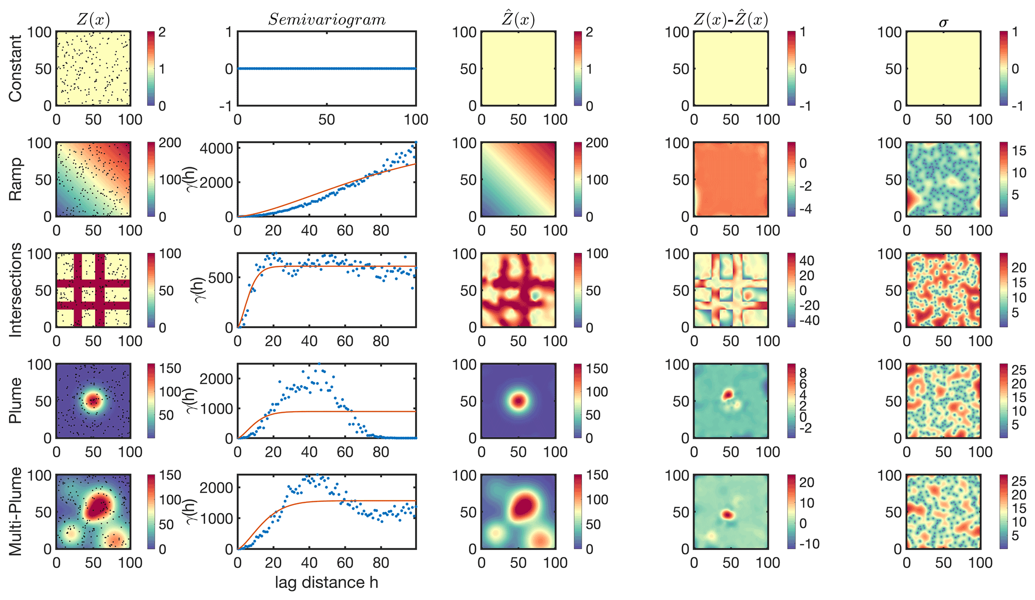
Figure 1 First column: five theoretical fields randomly sampled with 200 points (dots), namely, a constant field (C1), a ramp starting from zero in the lower left to higher values in the upper right (C2), an intersection with concentrated values in four corridors (C3), a Gaussian plume placed in the center (C4), and multiple Gaussian plumes spread over the entire domain (C5). Second column: the corresponding isotropic semivariograms computed based on Eq. (2); the red line shows the stable Gaussian fitted to the semivariogram based on the Levenberg–Marquardt method. Third column: the kriging estimate at the same resolution of the truth (i.e., 1×1) based on Eq. (6). Fourth column: the difference between the estimate and the truth. Fifth column: the kriging standard error based on Eq. (11).

As for C1, the uniformity results in a constant semivariogram leading the estimation to be identical to the truth. This estimation signifies the unbiased characteristic of ordinary kriging. C1 is never met in reality; however, it is possible to assume some degree of uniformity among data restrained to background values; a typical example of this can be seen in the spatial distribution of a number of trace gases in pristine environments such as NO₂ (e.g., Wang et al., 2020) and HCHO (Wolfe et al.,  2019). Under this condition, any data point within the field (i.e., the satellite footprint) can be assumed to be representative of the spatial variability in truth.

Concerning C2, the semivariogram shows a linear shape, meaning data points at larger distances exhibit larger differences. Generally geophysical samples are uncorrelated at large distances; thereby one expects the semivariogram to increase more slowly as the distance increases. The steady increase in γ(h) is indicative of a systematic drift in the data invalidating the assumption of m(x)=a₀. In many applications, a simple polynomial can explain m(x) and subsequently be subtracted from the data points. An example of this problem is tackled by Onn and Zebker (2006); it concerns the spatial variability of water vapor columns measured by GPS signals. Onn and Zebker (2006) observed a strong relationship between the water vapor columns and GPS altitudes resulting from the vertical distribution of water vapor in the atmosphere. Because of this complication, a physical drift model describing the vertical dependency was fit and removed from the measurements so that they could focus on the horizontal fluctuations. In terms of C2, one can effortlessly reproduce Z(x) by fitting a three-dimensional plane to barely three samples, indicating that the semivariogram is of little use.

C3 is an example of an extremely inhomogeneous field manifested in the stabilized semivariogram at a value of γ∼500, called the sill (Chilès and Delfiner, 2009), indicating insignificant information (variance) from the samples beyond this distance (∼20), called the range. Range is defined as the separation distance at which the total variance in data is extracted. The smaller the range is, the more heterogeneous the samples will be. While the estimated field roughly captures the shape of the intersections, it is spatially distorted at places with relatively sparse data points. The kriging model error is essentially a measure of the density of information. It converges to zero in the sample location and diverges to large values in gaps.

C4 is a close example of a point source emitter with faint winds and turbulence. The semivariogram exhibits a bell shape. As samples get further from the source, the variance diverges, stabilizes, and then sharply decreases. This is essentially because many data points with low values, apart from each other, have negligible differences. This tendency is recognized as the hole effect, which is characterized for high values to be systemically surrounded by low values (and vice versa). It is possible to mask this effect by fitting a semivariogram model stabilizing at a certain sill (like the one in Fig. 1). Nonetheless, if the semivariogram shows periodic holes, the fitted model should be modified to a periodic cosine model (Pyrcz and Deutsch, 2003).

The last case, C5, shows a less severe case of the hole effect previously observed in C4. This is due to the presence of more structured patterns in different parts of the domain. The range is roughly twice as large as the previous case (C4), denoting that there is more information (variance) among the samples at larger distances. A number of experiments using this particular case will be discussed in the following subsections.

2.2.2 Sensitivity to the number of samples

It is often essential to optimize the number of samples used for kriging. The kriging estimator somewhat recognizes its own capability at capturing the spatial variability through Eq. (11). Thus, if the target is spatially too complex and/or the samples are too limited, the estimator essentially informs that $\widehat{Z}\left(x_{\mathrm{0}}\right)$ is unreliable through large variance. However, there is a caveat; Y(x) must be a Gaussian random model with a zero mean so that kriging can capture the statistical distribution of $\widehat{Z}$ given the data points. Except this case, the kriging variance can either be underestimated or overestimated depending on the level of skewness of the statistical distribution of Y(x) (Armstrong, 1994). Figure 2 shows the kriging estimation for C5 using 5, 25, 50, 100, and 500 random samples in the entire field. Immediately apparent is a better description of the semivariogram when a larger number of samples is used, which in turn results in a better estimation of Z(x). The optimum number of samples to reproduce Z(x) depends on the requirement for the relative error ($\mathit{\sigma }/Z\left(x\right))$ being met at a given location.

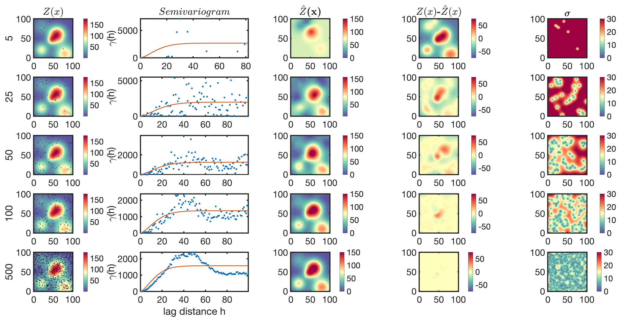
Figure 2 First column: the multi-plume case (C5) randomly sampled with a different number of samples (5, 25, 50, 100, and 500); second column: the corresponding isotropic semivariogram; third column: the kriging estimate; fourth column: the difference between the estimate and the truth; and fifth column: the kriging standard error.

2.2.3 Sensitivity to the tessellation of samples

A common application of kriging is to optimize the tessellation of data points for a fixed number of samples to achieve a desired precision. In real-world practices, the objective of such optimization is very purpose-specific; for example, one might prefer a spatial model representing a certain plume in the entire domain. Different ways for data selection exist (e.g., Rennen, 2008), but for simplicity, we focus on four categories: purely random, stratified random, a uniform grid, and an optimized tessellation. Figure 3 demonstrates the estimation of C5 using 25 samples chosen based on those four procedures.

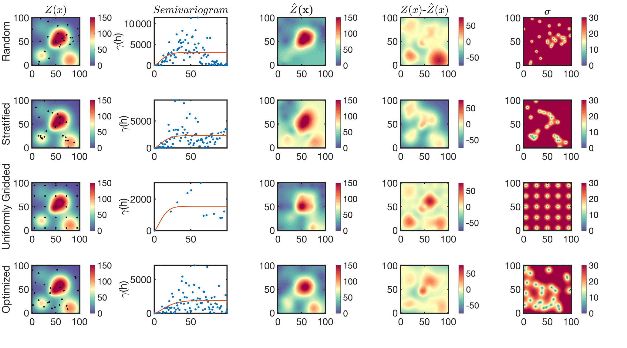
Figure 3 The multi-plume case (C5) randomly sampled by four different sampling strategies using a constant number of samples (25). The sampling strategies include purely random (first row), stratified random (second row), uniform grids (third row), and an optimized tessellation proposed based on kriging (fourth row). Columns represent the truth, the isotropic semivariogram, the kriging estimate, the difference between the estimate and the truth, and the kriging standard error.

Concerning the random selection, the lack of samples over two minor plumes causes the estimation to deviate largely from the truth. While a random selection may seem to be practical because it is independent of the underlying spatial variability, it can suffer from undersampling issues, thus being inefficient. As a remedy, it might be advantageous to group the domain into similar zones and randomly sample from each, which is commonly known as stratified random selection. We classify the domain into four zones by running the k-mean algorithm on the magnitudes of Z(x) (not shown) and randomly sample six to seven points from each one (total 25). We achieve a better agreement between the estimated field and the truth because we exploited some prior knowledge (here the contrast between low and high values).

As for the uniform grid, we notice that there are fewer data points in the semivariogram stemming from redundant distances, which is indicative of correlated information. Nonetheless, if the desired tessellation is neutral with regard to location, meaning that all parts of the domain are of equal scientific interest, the uniform grid is the most optimal design for the prediction of Z(x) under an ideally isotropic case. A mathematical proof for this claim can be found in Chilès and Delfiner (2009).

To execute the last experiment, we select 25 random samples for 1000 times and find the optimal estimation by finding the minimum sum of $\mathrm{|}\widehat{Z}\left(x_{\mathrm{0}}\right)-Z\left(x\right)\mathrm{|}$. It is worth mentioning that the optimized tessellation is essentially a local minimum based on 1000 kriging attempts. The optimized location of samples seems to be more clustered over areas with large spatial gradients. Not too surprisingly, we observe the smallest discrepancy between the estimation and the truth.

A lingering concern over the application of these numerical experiments is that the truth is assumed to be known. The truth is never known; this means we may never exactly know how well or poorly the kriging estimator is performing. However, it is highly unlikely for some prior understandings or expectations of the truth to be absent. If this is the case, which is rare, a uniform grid should be intuitively preferred to deliver the local estimations of average values in uniform blocks. In contrast, if the prior knowledge is articulated by previous site visits, model predictions, theoretical experiments, pseudo observations, or other relevant data, the tessellation needs to be optimized.

It is important to recognize that the uncertainties associated with the prior knowledge directly affect the level of confidence in the final answer. Accordingly, the prior knowledge error should ultimately be propagated to the kriging variance. The determination of the prior error is often done pragmatically. For example, if the goal is to design the location of thermometer sites to capture surface temperature during heat waves using a yearly averaged map of surface temperature, it would be wise to specify a large error with this specific prior information to play down the proposed design. This is primarily because the averaged map underrepresents such an atypical case. A possible extension of this example would be to use a weather forecast model with quantified errors capable of capturing retrospective heat waves. Although a reasonable forecast in the past does not necessarily guarantee a reasonable one in the future, it is rational to assume for the uncertainty with a new tessellation design using the weather model forecast to be lower than that using the averaged map.

A general roadmap for the data tessellation design is shown in Fig. 4. As proven in Chilès and Delfiner (2009), if the field is purely isotropic, the uniform grid is the most intuitive sensible choice when the prior information on the spatial variability is lacking. When the prior knowledge with quantified errors is available, an optimum tessellation can be achieved by running a large number of kriging models with suitable γ(h) and picking the one yielding the minimum difference between the prior knowledge and the estimation. The choice of the cost function (here L1 norm) is purpose-specific. For example, if the reconstruction of a major plume was the goal, using a weighted cost function, geared towards capturing the shape of plume, would be more appropriate.

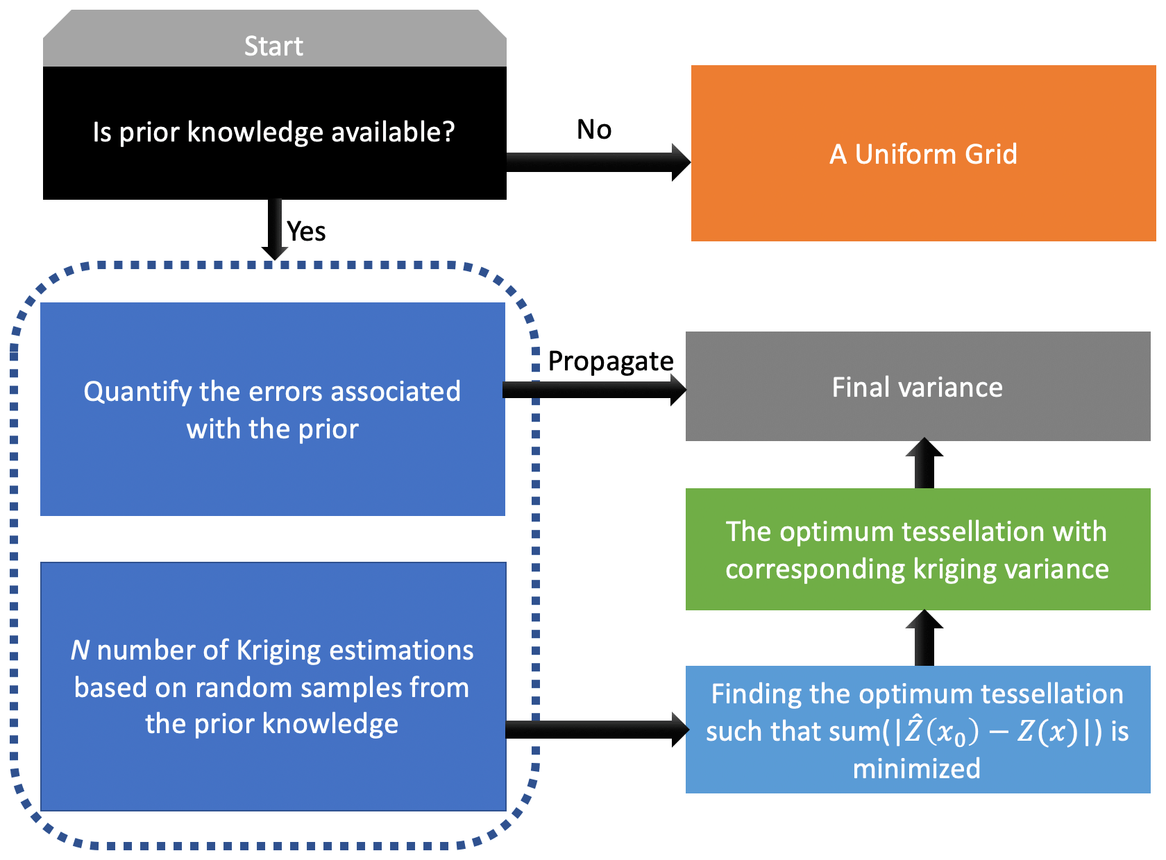
Figure 4 A schematic illustrating a framework for optimum sampling (tessellation) strategy. The prior knowledge refers to any data being capable of describing our quantity of interest including site visits, theoretical models, satellite observations, and emissions.

2.2.4 Sensitivity to the grid size

A kriging model can estimate a geophysical quantity at a desired location considering the data-driven spatial variability information. Since the kriging model is practically in a continuous form, the desired locations can be anywhere within the field of V. A question is whether or not it is necessary to map the data onto a very fine grid. There is a trade-off between the computational cost and the accuracy of the interpolated map. The range of the underlying semivariogram helps in finding the optimal solution. The greater the range is (i.e., a more homogeneous field), the less important to map the data in a finer grid are.

Figure 5a depicts an experiment comparing the estimates of C2 at different grid sizes with the truth. The departure of the estimate from the truth is rather negligible for several coarse grids (e.g., 10×10). The homogeneous field, manifested by the large range (Fig. 1), allows for a reasonable estimation of Z(x) at coarse resolutions with inexpensive computational costs. Figure 5b shows the same experiment but on C5 with the optimized tessellation. As opposed to the previous experiment, the estimate substantially diverges from the truth when increasing the grid size, suggesting that a finer resolution should be used for fields with smaller ranges (i.e., heterogeneous fields).

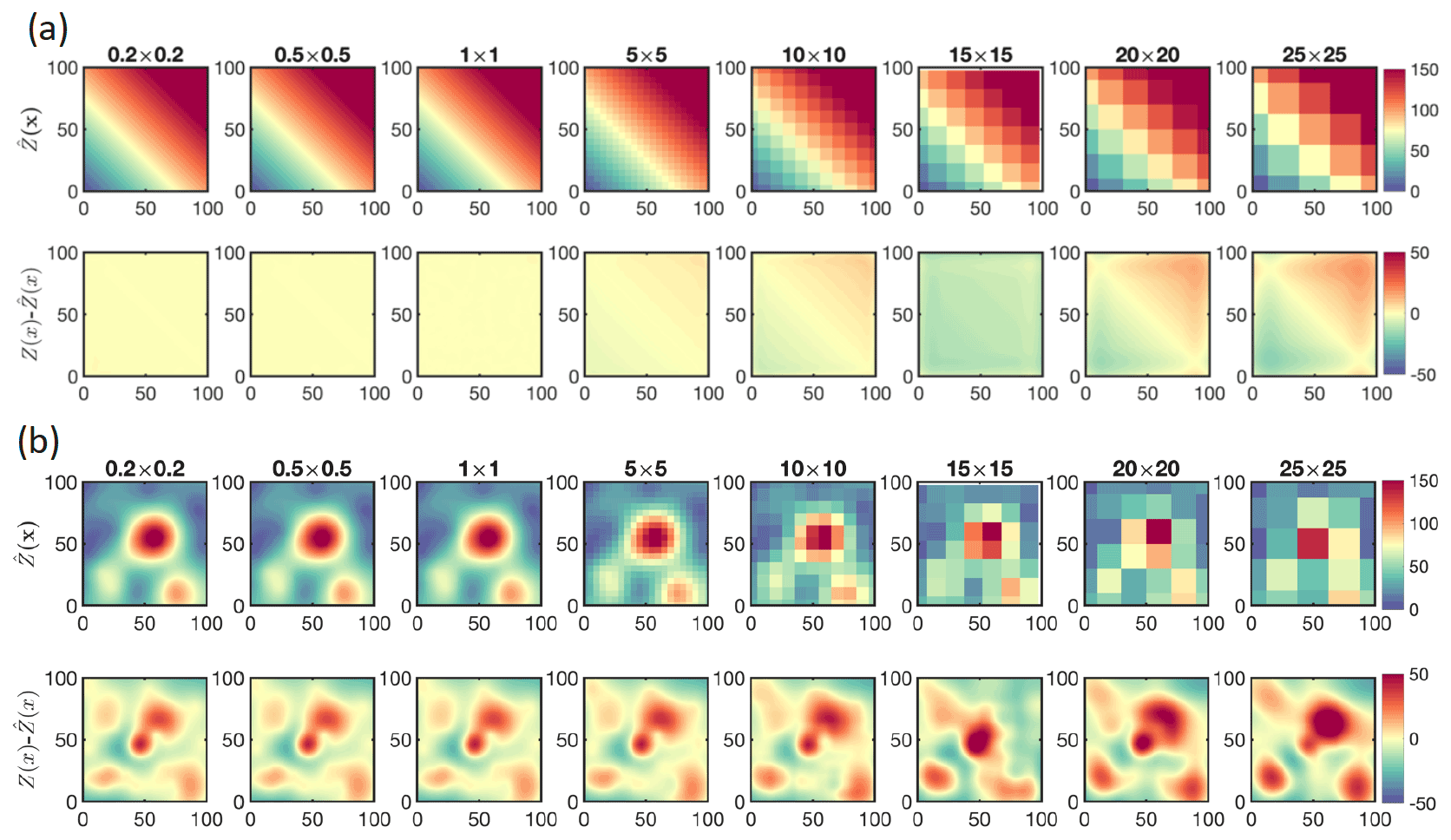
Figure 5 Finding an optimum grid size for kriging. (a) The kriging estimates of the ramp (C2) at different grid resolutions ranging from 25×25 pixel to 0.2×0.2. (b) The kriging estimates of the multi-plume (C5) with optimized samples shown in Fig. 3 for different grid resolutions. C2 is more homogeneous than C5; as a result, it is less sensitive to the resolution of the kriging estimate. The optimum grid resolution for C2 is 10×10, whereas it is 1×1 for C5. These numbers are based on observing the negligible difference (<1 %) between the kriging estimate at the optimum resolution and the one computed at a finer-resolution step. We call the optimum output for C5 as C5opt.

The complexity of directly using the range for choosing the optimal grid size arises from the fact that the level of spatial homogeneity can vary within the domain. In fact, the range is derived from a semivariogram model representing a crude estimate of varying ranges occurring at various scales. It is intuitively clear that depending on the degree of heterogeneity, which is spatiotemporally variable, the grid size needs to be adaptively adjusted (Bryan, 1999). For the sake of simplicity, but at a higher computational cost, we adopt a numerical solution which is to first simulate on a coarse grid and then on a finer one until the difference with respect to the previous grid size across all pixels reaches an acceptable value (<1 %). We name this output (1×1) with the optimized tessellation for C5 as C5opt.

3 Comparison of points to satellite pixels

3.1 Synching the scales between the gridded field and satellite pixels

To minimize the complications of different spatial scales between two gridded data, we first need to upscale the finer-resolution data to match the coarse ones. In case of numerical chemical transport or weather forecast models, the size of the grid box is definitive. Likewise, a satellite footprint, mainly dictated by the sensor design, the geometry, and signal-to-noise requirements (Platt et al., 2021), is known. However, the grid size of the kriging estimation is a variable subject to optimization which has been discussed previously. When we compare the grid size of the kriging estimate to that of a satellite (or a model), three situations arise: first, the kriging spatial resolution is coarser than the satellite, a condition occurring when either the field is homogeneous or the field is undersampled. In situations where the field is homogeneous (γ(h)≅0), it is safe to directly compare the data points to the satellite measurements without having to use kriging. If the undersampling is the case (see Fig. 2 with 5 samples), it is sensible to first investigate if the field is homogeneous within the satellite footprint using different data (if any). If the homogeneity is met, we can compare two datasets either without kriging or, to match the size of kriging grid cell, with the satellite footprint and statistically involve the kriging variance in the comparison (discussed later); nonetheless, the kriging estimate beyond the location of samples must be used with extra caution because their variance very quickly departs from zero to extremely large numbers (see Fig. 1). Thus, there is a compromise between increasing the number of paired samples between two datasets and enhancing the level of confidence in statistics. If independent observations suggest that there might be large heterogeneity within a satellite footprint, it is strongly advised against quantitatively comparing the points to the satellite observations. Second, the number of samples is fewer than three observations in the field, so it is in principle impossible to build a semivariogram. Validating a satellite under this condition is prone to misinterpretation because the spatial heterogeneity cannot be modeled. Nonetheless, if one presumes a good degree of homogeneity within the sensor footprint (such as very high-resolution remote sensing airborne data), the direct comparison of point measurements might be possible. Third, the satellite footprint is coarser than the kriging estimate. Under this condition, we upscale the kriging map to match the spatial resolution of the satellite using

$$\begin{array}{}\text{(12)}& {\widehat{Z}}_{\mathrm{c}}={\widehat{Z}}_{\mathrm{f}}\ast S=\int {\widehat{Z}}_{\mathrm{f}}\left(x\right)S(x-y)\mathrm{d}y,\end{array}$$

where S is the spatial response function, ${\widehat{Z}}_{\mathrm{c}}$ is the coarse kriging field, $<*>$ is the convolution operator, y is shift, and ${\widehat{Z}}_{\mathrm{f}}$ is the fine field. In discrete form we can rewrite Eq. (12) in

$$\begin{array}{}\text{(13)}& {\widehat{\mathbf{Z}}}_{\mathrm{c}}\left[ij\right]=\sum _m\sum _n{\widehat{\mathbf{Z}}}_{\mathrm{f}}\left[i-m,j-n\right]\mathbf{S}[m,n],\end{array}$$

where m and n are the dimension of the response function. The mathematical formulation of S[m,n] for a number of satellites can be represented by two-dimensional super Gaussian functions as discussed in Sun et al. (2018). Atmospheric models have a uniform response to the simulated values within a grid box; therefore, $\mathbf{S}[m,n]=\frac{\mathrm{1}}{m\times n}{\mathbf{J}}_{m,n}$, where J is the matrix of ones. In the same way, the kriging variance should be convolved through

$$\begin{array}{}\text{(14)}& {\mathit{\sigma }}_{\mathrm{c}}^{\mathrm{2}}[i,j]=\sum _m\sum _n{\mathit{\sigma }}_{\mathrm{f}}^{\mathrm{2}}\left[i-m,j-n\right]{\mathit{S}}^{\mathrm{2}}[m,n],\end{array}$$

where a superscript of 2 denotes squaring, and ${\mathit{\sigma }}_{\mathrm{c}}^{\mathrm{2}}$ and ${\mathit{\sigma }}_{\mathrm{f}}^{\mathrm{2}}$ are the kriging variance matrices in the coarse and the fine grids, respectively.

To demonstrate the upscaling procedure, we use C5opt (1×1) and upscale it at six grid sizes (m,m) of 5×5, 10×10, 15×15, 20×20, 25×25, and 30×30. For simplicity, we consider $\mathbf{S}=\frac{\mathrm{1}}{m^{\mathrm{2}}}{\mathbf{J}}_{m,m}$; this spatial response function results in averaging the values in the grid boxes. Figure 6 shows the resultant map overplotted with the samples along with the error estimation. Two tendencies from this experiment can be identified: first, the discrepancy of the point data and $\widehat{Z}$ is becoming more noticeable as the grid size grows; this directly speaks to the notion of the spatial representativeness; large grid boxes are less representative of subgrid values. Second, the gradients of the field along with the estimation error become smoother primarily due to convolving the field with the spatial response function, which acts as a low pass filter.

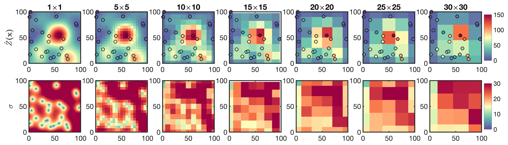
Figure 6 First row: C5Opt outputs convolved with an ideal box kernel with different sizes (1×1 up to 30×30) overlaid by the C5Opt optimum samples. Second row: the associated kriging errors convolved with the same kernel. The coarser the resolution is, the larger the discrepancy between the samples and the estimates is.

We further directly compare $\widehat{Z}$ to the samples (i.e., observations) shown in Fig. 7. We see an excellent comparison between $\widehat{Z}$ at 1×1 resolution with the observations underscoring the unbiasedness characteristic of the kriging estimator. Conversely, the upscaled field gradually diverges from the observations. This divergence is the problem of scale.

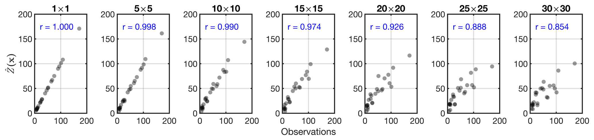
Figure 7 Illustrating the problem of spatial scale: comparisons of the kriging estimates at seven different spatial scales with the samples used for the C5opt estimation. The perceived discrepancies are purely due to the spatial representativeness.

3.2 Point to pixel vs. pixel to pixel

To elaborate on the problem of scale, we design an idealized experiment theoretically validating pseudo satellite observations against some pseudo point measurements. The pseudo satellite observations are created by upscaling the C5 truth (Z) to 30×30 grid footprint considering $\mathbf{S}=\frac{\mathrm{1}}{m^{\mathrm{2}}}{\mathbf{J}}_{m,m}$, meaning that the satellite is observing the truth but in a different scale (Fig. S1 in the Supplement). The pseudo point measurements are the ones used for C5opt. Figure 8a shows the direct comparison of the satellite pixel with the point observations. By ignoring the fundamental fact that these two datasets are inherently different in nature, displaying the same geophysical quantity at different scales, we observe a perceived discrepancy (r²=0.64). The comparison suggests a wrong conclusion that the satellite observations are biased low. This discrepancy is unrelated to any observational or physical errors, rendering any physical interpretation of the comparison biased due to spatial-scale differences in the datasets. Figure 8b depicts the comparison of each grid box of the upscaled kriging estimate (30×30) with that of the satellite. This direct comparison shows a strong degree of agreement (r²=0.98), shaking off the erroneous idea of directly comparing point data to gridded data when the field exhibits substantial spatial heterogeneity.

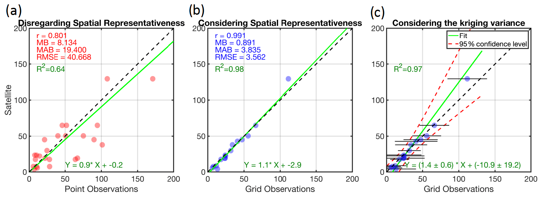
Figure 8 (a) The direct comparison of pseudo observations of a satellite observing the C5 case at 30×30 resolution vs. the 25 samples used for C5opt. (b) Same for the y axis, but the point samples are transformed to grid boxes using kriging convolved with the satellite spatial response function (ideal box with 30×30 kernel size). The differences in statistics between these two experiments speak to the problem of scale. Panel (b) ignores the kriging errors but panel (c) incorporates them using a Monte Carlo method. Note that the best linear fit has changed, indicating that the consideration of the kriging variance is critical. MB: mean bias (point minus satellite); MAB: mean absolute bias; RMSE: root mean square error; R²: coefficient of determination.

Yet, the comparison misses an important point: the kriging estimate is considered error-free. We attempt to incorporate the kriging variance through a Monte Carlo linear regression method. Here, the goal is to find an optimal linear fit $(y=ax+b+\mathit{\epsilon })$ such that ${\mathit{\chi }}^{\mathrm{2}}=\sum \frac{{\left[y-f(x_i,a,b)\right]}^{\mathrm{2}}}{{\mathit{\sigma }}_y^{\mathrm{2}}+a^{\mathrm{2}}{\mathit{\sigma }}_x^{\mathrm{2}}}$ is minimized. ${\mathit{\sigma }}_y^{\mathrm{2}}$ and ${\mathit{\sigma }}_x^{\mathrm{2}}$ are the variances of y (here the satellite) and x (the kriging variance), respectively. We set the errors of y to zero and randomly perturb the errors of x based on a normal distribution with zero mean and a standard deviation equal to that of kriging estimate 15 000 times. The average of optimized a and b coefficients derived from each fit is then estimated, and their deviation at the 95 % confidence interval assuming a Gaussian distribution is determined. Figure 8b and c show the linear fit with and without considering the kriging error estimate. The linear fit without involving the kriging error gives a strong impression that it is nearly perfect, following closely to the paired observations. This is essentially explainable by the primary goal of χ², which is to minimize the L2 norm of residuals $(y-f(x_i,a,b\left)\right)$, portraying a very optimistic picture of the satellite validation. The linear fit considering the kriging errors is different. The uncertainties associated with a and b are larger since x is variable (shown in horizontal error bars). The optimal fit gravitates towards the points with smaller standard deviations as they impose a larger weight. The confidence in the linear fit at higher values is lower due to their errors being large. This fit is a more realistic portrayal of the satellite validation.

Figure 9 summarizes the general roadmap for satellite (and model) validations against point measurements. To fit the semivariogram with at least two parameters, we are required to have three samples at minimum. Therefore, it is implausible to derive the spatial information from the point data where sampling is extremely sparse (<3 samples within the field). The only case of directly comparing point and satellite pixels is when the field within satellite footprint or the field in general is rather homogeneous, which is confirmed by independent data/models. Having more samples allows us to acquire some information on the spatial heterogeneity. The information carried by the data is considered more and more robust when increasing the number of samples. Subsequently, the kriging map along with its variance derived from a reasonable semivariogram at an optimized grid resolution should be convolved with the satellite response function so that we can conduct an apples-to-apples comparison. A real-world example on the satellite validation will be shown later.

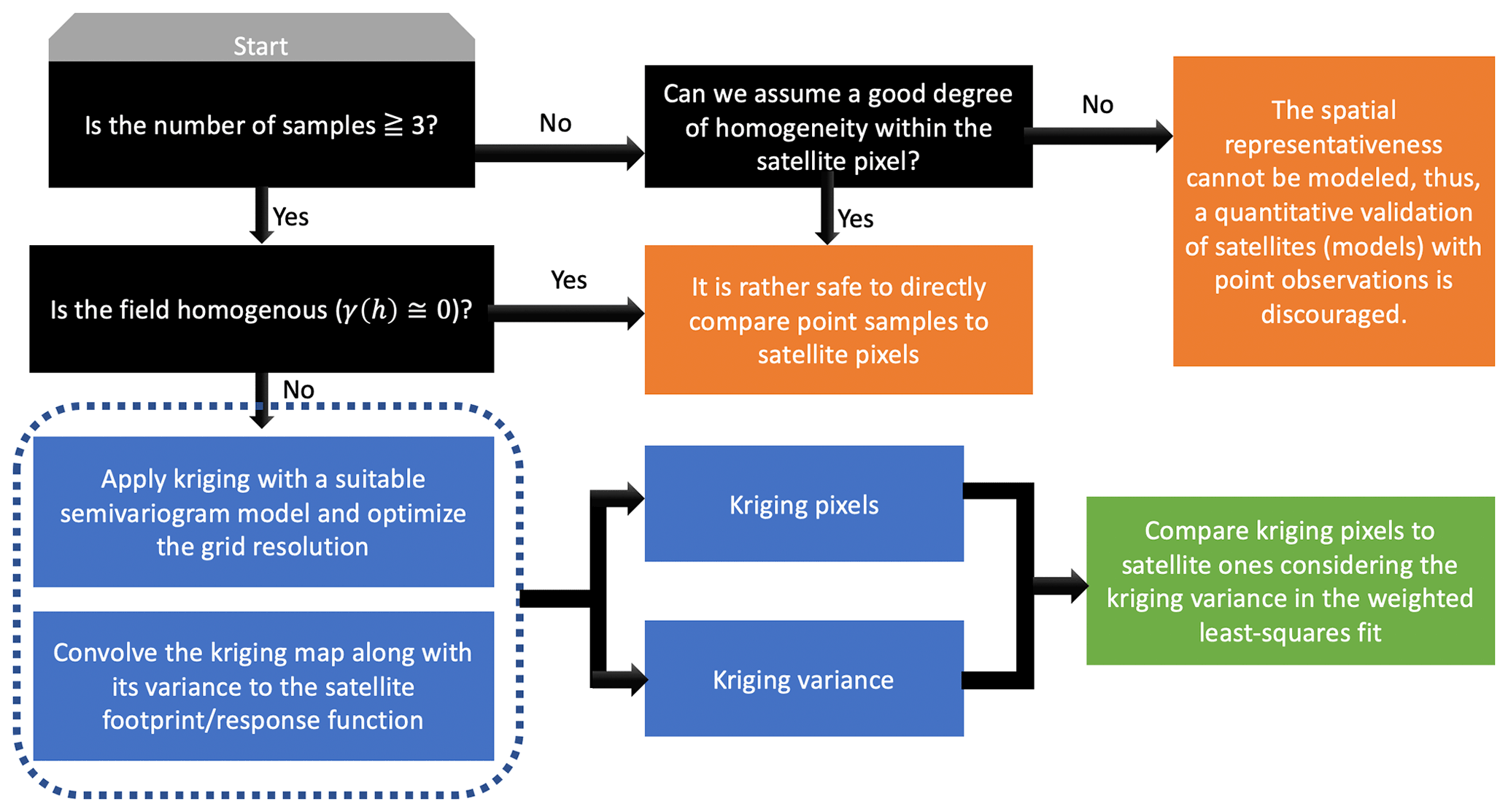
Figure 9 The proposed roadmap for transforming pointwise measurements to gridded data in satellite (model) validation.

4 Real-world experiments

4.1 Spatial distribution of NO₂

We begin with focusing on tropospheric NO₂ columns observed by the TROPOMI sensor (Copernicus Sentinel data processed by ESA and Koninklijk Nederlands Meteorologisch Instituut, KNMI, 2019; Boersma et al., 2018) at ∼ 13:30 LST. We choose NO₂ primarily due to its spatial heterogeneity (e.g., Souri et al., 2018; Nowlan et al., 2016, 2018; Valin et al., 2011; Judd et al., 2020). We oversample good-quality pixels (qa_flag >0.75) through a physical-based gridding approach (Sun et al., 2018) over Texas at 3×3 km² resolution in four seasons in 2019. We extract samples by uniformly selecting the NO₂ columns in the center of each 30×30 km² block. The semivariogram along with its model is calculated, and then we krige the samples. Figure 10 shows the NO₂ columns map for four different seasons, the semivariogram, the kriging estimates, and the differences between the estimate and the field. High levels of NO₂ are confined to cities, indicating that the sources are predominantly anthropogenic. Wintertime NO₂ columns are larger than summertime mainly due to meteorological conditions and the OH cycle, the major sink of NO₂. All semivariograms exhibit the hole effect. This is because of high values of NO₂ being systematically surrounded by low values. Regardless of the season, we fit the stable Gaussian to variances at distances smaller than 2.5^∘ (∼275 km²). The b parameter in Eq. (4) explaining the length scale is found to be 0.94, 0.88, 0.71, and 0.83^∘ for DJF, MAM, JJA, and SON, respectively. These numbers strongly coincide with the seasonal lifetime of NO₂ (Shah et al., 2020); wintertime NO₂ columns are spatially more uniform around the sources; thus, in relative sense, they are more homogeneous (spatially correlated) than those in warmer seasons. On the other hand, the shorter NO_x lifetime in summer results in a steeper gradient of NO₂ concentrations. This tendency should not be generalized because transport and various NO_x sources including biomass burning, soil emissions, and lightning can have large spatiotemporal variability resulting in different length scales at different times of a year. The differences between the kriging estimate and the field show some spatial structures indicating that NO₂ is greatly heterogenous.

Figure 10 First column: the spatial distribution of TROPOMI tropospheric NO₂ columns oversampled in four different seasons in 2019 at 3×3 km² spatial resolution. Second column: the corresponding semivariogram from samples selected from uniform 30×30 km² blocks (shown with black dots in the first column) along the fitted stable Gaussian model (red line). Third column: the kriging estimates. Fourth column: the kriging estimates' differences with respect to the observations.

4.2 Optimized tessellation over Houston

The preceding TROPOMI data enabled us to optimize a tessellation of ground-based point spectrometers over Houston. Our goal here is to propose an optimized network for winter 2021 given our knowledge on the spatial distribution of NO₂ columns in winter 2019 measured by TROPOMI. The assumption of using a retrospective NO₂ field for informing a hypothetical future campaign is not entirely unrealistic. If we have a consistent number of pixels from TROPOMI between two years, it is unlikely for the spatial variance of NO₂ to be substantially different for the same season. We follow the framework proposed in Sect. 2.2.3 involving randomly selecting samples from the field (for 50 000 iteration) and calculating kriging estimates for a given number of spectrometers. We then choose the optimum tessellation based on the minimum sum of $\mathrm{|}\widehat{Z}\left(x_{\mathrm{0}}\right)-Z\left(x\right)\mathrm{|}$.

Figure 11 shows the optimized tessellation given 5, 10, 15, and 20 spectrometers over Houston. The Houston plume is better represented with more samples being used. All cases share the same feature; the optimized samples are clustered in the proximity or within the plume. This tendency is clearly intuitive. We are required to place the spectrometers in locations where a substantial gradient (variance) in the field is expected. The difference between the kriging estimate and the TROPOMI observations using 20 samples does not substantially differ in comparison to the one using 15 samples. Therefore, to keep the cost low, a preferable strategy is to keep the number of spectrometers as low as possible while achieving a reasonable accuracy. Based on the presented results, the optimized tessellation using 15 samples is preferred among others because it achieves roughly the same accuracy as the one with 20 samples.

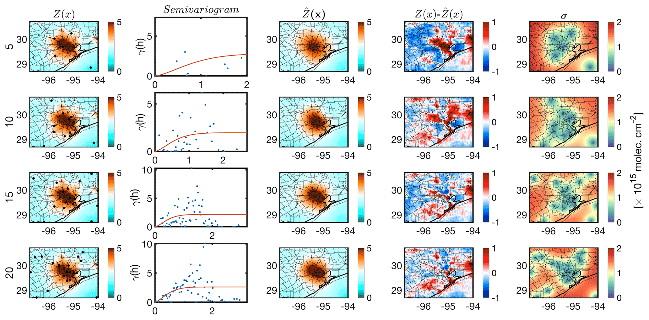
Figure 11 Finding an optimum sample tessellation for wintertime over Houston given a different number of spectrometers (5, 10, 15, and 20).

4.3 Validating OMI tropospheric NO₂ columns during the DISCOVER-AQ 2013 campaign using Pandora

In order to understand ozone pollution (e.g., Mazzuca et al., 2016; Pan et al., 2017b, 2015), characterize anthropogenic emissions (Souri et al., 2016, 2018), and validate satellite data (Choi et al., 2020), an intensive air quality campaign was carried out in September 2013 over Houston (DISCOVER-AQ). The campaign encompassed a large suite of Pandora spectrometer instrument (PSI) (11 stations) measuring total NO₂ columns with a high precision (2.7×10¹⁴ molecules cm⁻²) and a moderate nominal accuracy (2.7×10¹⁵ molecules cm⁻²) under the clear-sky condition (Herman et al., 2009). We remove the observations with an error of >0.05 DU, contaminated by clouds, and averaged them over the month of September at 13:30 LST (±30 min). We attempt to validate OMI tropospheric NO₂ columns version 3.0 (Bucsela et al., 2013) refined in Souri et al. (2016) with the 4 km model profiles. The OMI sensor resolution varies from 13×34 km² at nadir to $\sim \mathrm{40}\times \mathrm{160}$ km² at the edge of the scan line. Biased pixels were removed based on cloud fraction >0.2, terrain reflectivity >0.3, and main (xtrack) quality flags =0. Following Sun et al. (2018), we oversample high-quality pixels in the month of September 2013 over Houston at 0.2×0.2^∘ resolution. To remove the stratospheric contributions from PSI measurements, we subtract OMI stratospheric NO₂ ($\mathrm{2.8}\pm \mathrm{0.16}\times {\mathrm{10}}^{\mathrm{15}}$ molecules cm⁻²) from the total columns over the area. Figure 12 shows the monthly-averaged tropospheric NO₂ columns measured by OMI overplotted by 11 PSIs. The elevated NO₂ levels (up to $\sim \mathrm{6}\times {\mathrm{10}}^{\mathrm{15}}$ molecules cm⁻²) are seen over the center of Houston.

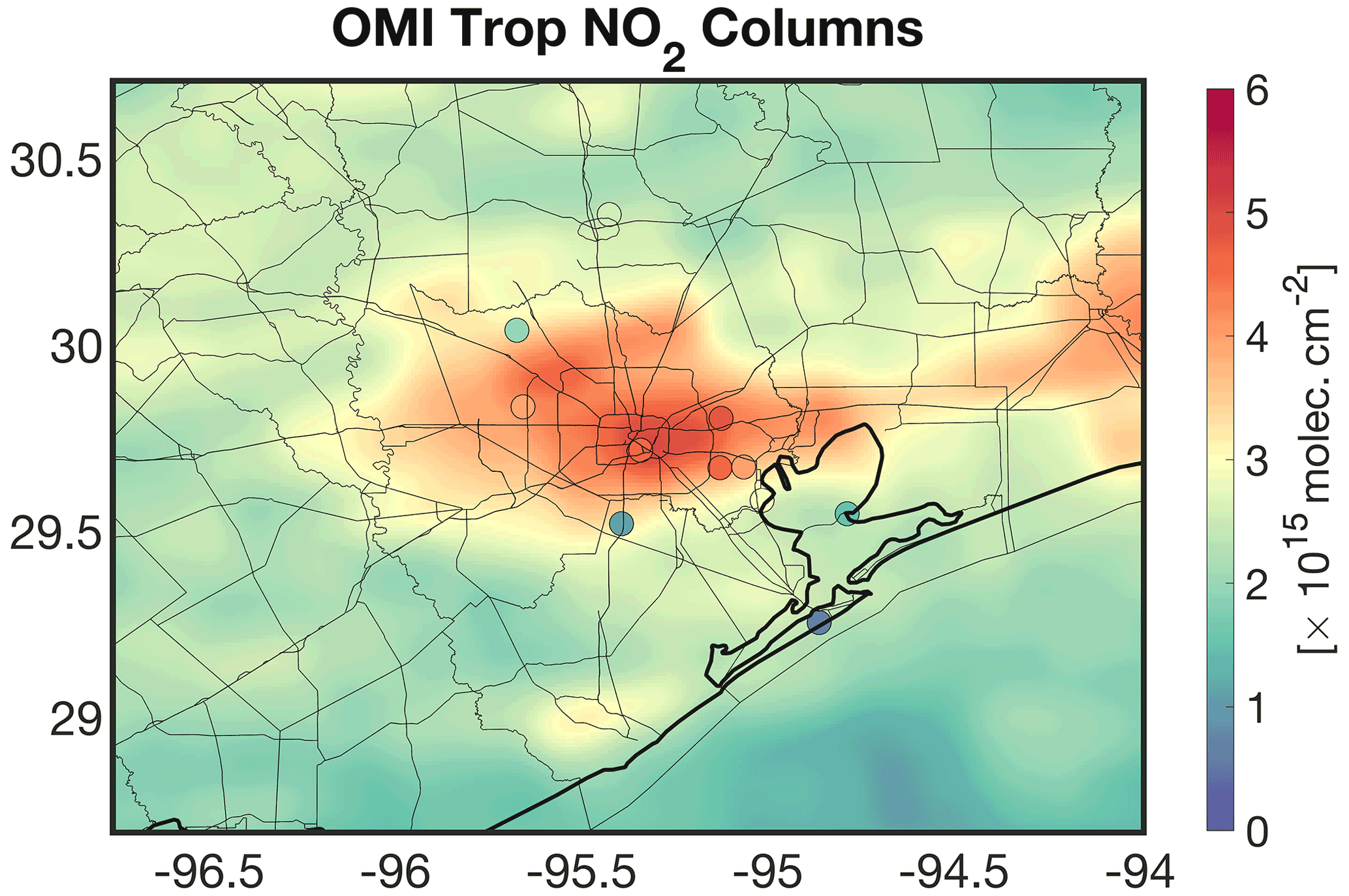
Figure 12 The spatial distribution of OMI tropospheric NO₂ columns oversampled at the resolution at 0.2×0.2^∘ over Houston in September 2013. The plot is overlaid by the surface Pandora spectrometer instrument averaged over the same month. The surface measurements originally measured the total columns; therefore, we subtract the stratospheric columns provided by the OMI data ($\mathrm{2.8}\pm \mathrm{0.16}\times {\mathrm{10}}^{\mathrm{15}}$ molecules cm⁻²) from the total columns to focus on the tropospheric part.

We then follow the validation framework shown in Figure 9 in which the number of point measurements and the level of heterogeneity are the main factors in deciding if we should directly compare them to the satellite pixels. Figure 13 shows the monthly-averaged PSI measurements along with the semivariogram and resulting kriging estimate at an optimized resolution ($\sim \mathrm{2}{\mathrm{km}}^{\mathrm{2}}=\mathrm{13}\mathrm{800}$ data over the entire region) and errors. The distribution of the semivariogram suggests that there is a strong degree of spatial heterogeneity, necessitating the use of kriging. We fit a stable Gaussian to the semivariogram, resulting in $\mathrm{2.23}\times \left(\mathrm{1}-e^{-(\frac{h}{\mathrm{0.19}}{)}^{\mathrm{1.5}}}\right)$. The spatial information (variance) levels off at 0.19^∘ (∼21 km), with a maximum variance equal to 2.23 molecules² cm⁻⁴. The measurements beyond this range (21 km) have a minimal weight due to this length scale. It is because of this reason that we see the kriging estimate converges to a fixed value at places being further than this range. The kriging errors of those grid boxes are constantly large (40 % relative error). The optimum grid size for kriging is found to be 2 km² (<1 % difference across all grid boxes). Subsequently, we use the super Gaussian spatial response function described in Sun et al. (2018) to convolve both the kriging estimate and error within (see Fig. S2). Figure 14 shows the differences between the kriging estimate and error before and after convolution. The response function (OMI pixel) tends to be on average coarser than 2 km², resulting in smoothing of both the kriging estimate and error.

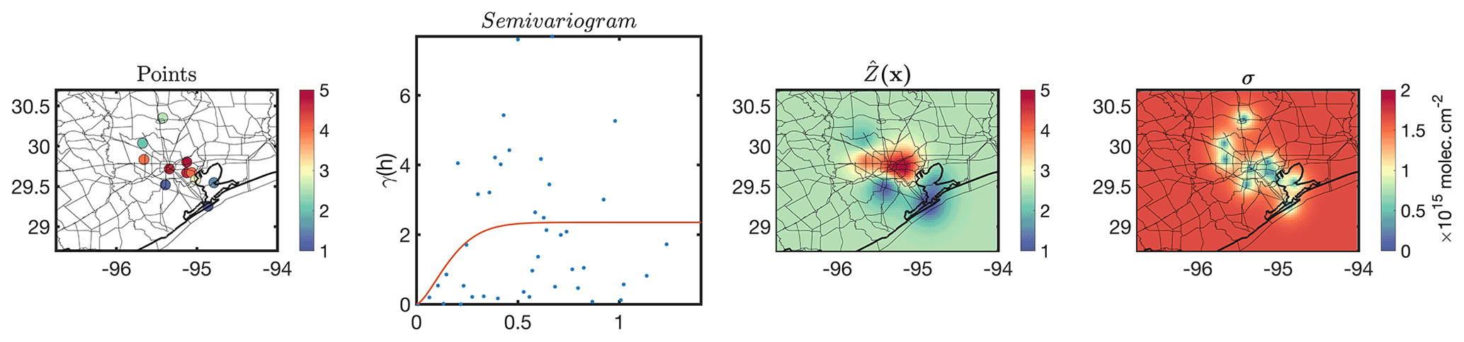
Figure 13 The Pandora tropospheric NO₂ measurements (made from subtracting the total columns from the OMI stratospheric NO₂ columns) during September 2013, the corresponding semivariogram, the kriging estimates, and the kriging standard errors. Note that the semivariogram suggests a large degree of spatial heterogeneity occurring at different spatial scales.

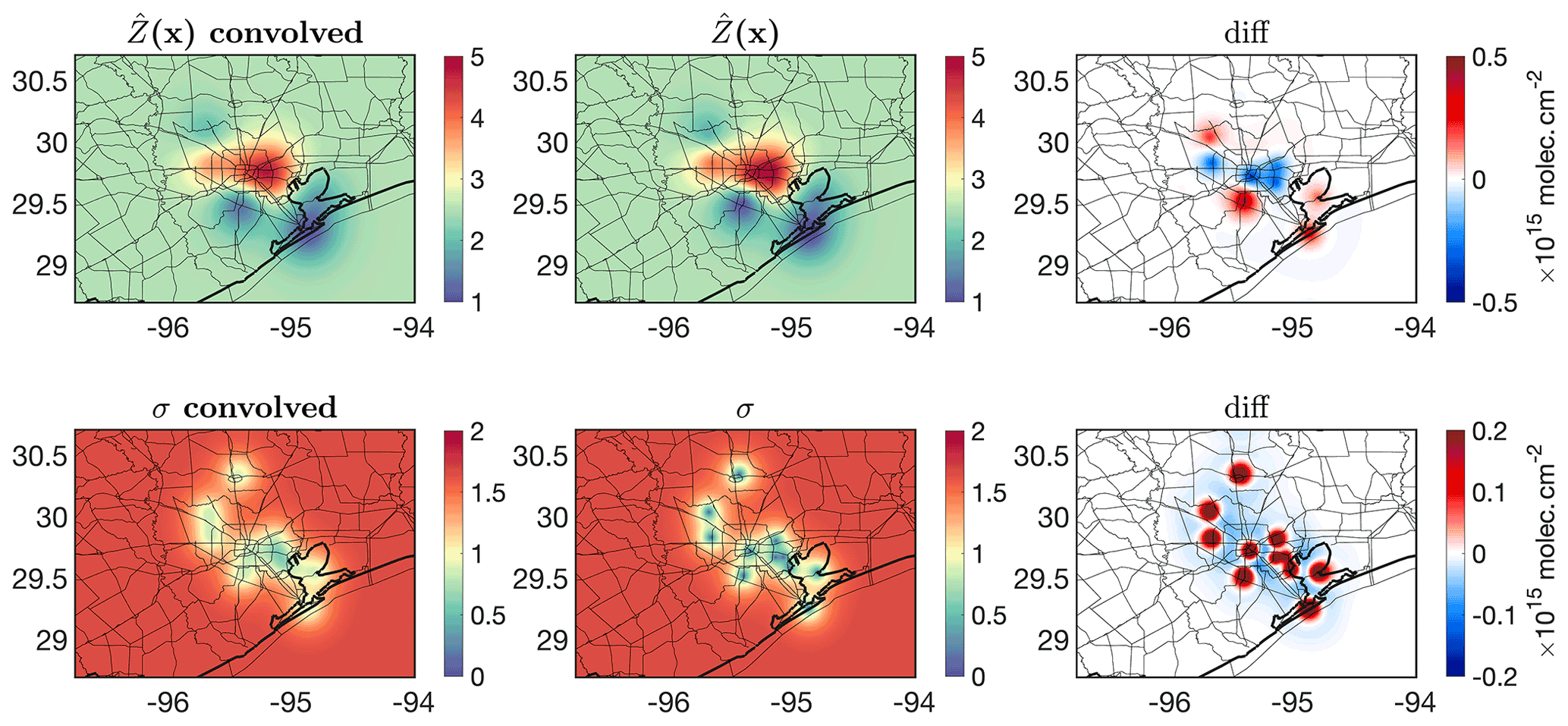
Figure 14 Convolving both kriging estimates and errors with the OMI spatial response function formulated in Sun et al. (2018). The differences against the pre-convolved fields are also depicted.

We ultimately conduct two different sets of comparison: directly comparing PSI to OMI pixels and comparing convolved kriged PSI to OMI. It is worth noting that PSI measurements are monthly-averaged; similarly, OMI data are oversampled on a monthly basis. In terms of the PSI, we only account for grid boxes whose kriging error is below 1.2×10¹⁵ molecules cm⁻² (1193 samples, 8 % of total kriging grid boxes). As for the grid-to-grid comparison, the kriging variance is considered in the linear polynomial fitted to the data through the Monte Carlo of the chi-square with 5000 iterations. The variability with the OMI stratospheric NO₂ columns (0.16×10¹⁵ molecules cm⁻²) is added to the PSI error for both analyses. The left and right panels of Fig. 15 show the comparisons. As for the direct comparison of actual points (PSI) to pixels (OMI), the PSI measurements indicate a deviation of the slope (r²=0.66) from the unity line. This suggests that there is an unresolved magnitude-dependent systematic error. The grid-to-grid comparison not only offers a clearer picture of the distribution of data points, but also it hints at the offset being rather constant ($\mathrm{0.66}\pm \mathrm{0.18}\times {\mathrm{10}}^{\mathrm{15}}$ molecules cm⁻²; r²=0.72). We also observe that the statistics between the satellite and the benchmark are moderately improved. This comparison in general provides an important implication: the varying offsets in a plume shape environment (high to low values) are not necessarily due to variable offsets in the satellite retrieval, as the kriging estimate suggests that those varying offsets in point-to-pixel comparison, manifested in slope =0.76, are a result of varying spatial scales.

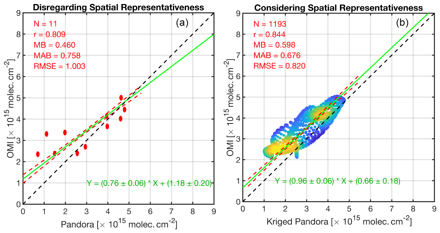
Figure 15 (a) The direct comparison of OMI tropospheric NO₂ columns with 11 pointwise Pandora measurements in September 2013 over Houston. (b) Same for the y axis, but the PSI measurements are translated to grid boxes using kriging convolved with the OMI spatial response function. PSI tropospheric NO₂ columns are estimated based on subtracting the OMI stratospheric NO₂ columns ($\mathrm{2.8}\pm \mathrm{0.16}\times {\mathrm{10}}^{\mathrm{15}}$ molecules cm⁻²) from the total columns. We only consider kriging estimates whose errors are below 1.2×10¹⁵ molecules cm⁻². The kriging variance is also considered using the Monte Carlo method applied on χ². The slope has improved after considering the modeled spatial representativeness. MB: mean bias (OMI vs. Pandora); MAB: mean absolute bias; RMSE: root mean square error.

5 Summary

There needs to be increased attention to the spatial representativity in the validation of satellite (model) against pointwise measurements. A point is the element of space, whereas satellite (model) pixels (grid box) are (at best) the product of the integration of infinitesimal points and a normalized spatial response function. If the spatial response function is assumed to be an ideal box, the resulting grid box will represent the average. Essentially, no justifiable theory exists to accept that the averaged value of a population should absolutely match with a sample, unless all samples are identical (i.e., a spatially homogeneous field). This glaring fact is often overlooked in the atmospheric science community. At a conceptual level, we are required to translate pointwise data to the grid format (i.e., rasterization). This can be done by modeling the spatial autocorrelation (or semivariogram) extracted from the spatial variance (information) among measured sample points. Assuming that the underlying field is a random function with an unknown mean, the best linear unbiased predictions of the field can be achieved by kriging using the modeled semivariograms.

In this study, we discussed methods for the kriging estimation of several idealized cases. Several key tendencies were observed through this experiment: first, the range corresponded to the degree of spatial heterogeneity; a larger range indicated the lower presence of heterogeneity. Second, the kriging variance explaining the density of information quickly diverged from zero to large values when the field exhibited large spatial heterogeneity. This tendency mandates increasing the number of samples (observations) for those cases. Third, while the semivariogram models were constructed from discrete pair of samples, they are mathematically in a continuous form. It is because of this reason that we determined the optimal spatial resolution of the kriging estimate by incrementally making the grids finer and finer until a desired precision (=1 %) was met.

The present study applied kriging to achieve an optimum tessellation given a certain number of samples such that the difference between our prior knowledge of the field, articulated by previous observations, models, or theory, and the estimation is minimal. Usually there is uncertainty about the prior knowledge that should be propagated to the final estimates. The optimum tessellation for a range of idealized and real-world data consistently voted for placing more samples in areas where the gradients in the measurements were significant such as those close to point emitters.

This study also revisited the spatial representativity issue; it limits the realistic determination of biases associated with satellites (models). In one experiment, we convolved the kriging estimate for a multi-plume field with a box filter but various sizes. The perfect agreement (r=1.0) between the samples (point) and kriging output (pixel) seen at a high spatial resolution gradually vanished with coarsening of the resolution of grid boxes (r=0.8). We also directly compared samples (point) with pseudo satellite observations (showing the truth) with a coarse spatial resolution, which led to a flawed conclusion about the satellite being biased low. We modeled the semivariogram of those samples, estimated the field using kriging, and convolved with the pseudo satellite spatial response function. The direct comparison of this output with that of the satellite showed a completely different story, suggesting that the data were rather free of any bias. A serious caveat with using a spatial model (here kriging) is that it consists of errors: the estimations that are further from samples are less certain. It is widely known that discounting the measurement/model errors in true straight-line relationship between data can introduce artifacts. To consider the kriging variance in the comparisons we employed a Monte Carlo method on chi-square optimization, which ultimately allowed us to not only provide a set of solutions within the range of the uncertainty of the kriging model, but also to assign smaller weights on gross estimates.

We further validated monthly-averaged Ozone Monitoring Instrument (OMI) tropospheric NO₂ columns using 11 Pandora spectrometer instrument (PSI) observations over Houston during NASA's DISCOVER-AQ campaign. A pixel-to-point comparison between two datasets suggested varying biases in OMI manifested in a slope far from the identity line. By contrast, the kriging estimate from the PSI measurements, convolved with the OMI spatial response function, resulted in an inter-comparison slope close to the unity line. This suggested that there was only a constant systematic bias ($\mathrm{0.66}\pm \mathrm{0.18}\times {\mathrm{10}}^{\mathrm{15}}$ molecules cm⁻²) associated with the OMI observations which does not vary with tropospheric NO₂ column magnitudes.

The central component of satellite and model validation is pointwise measurements. Our experiments paved the way for a clear roadmap explaining how to transform these pointwise datasets to a comparable spatial scale relative to satellite (model) footprints. It is no longer necessary to ignore the problem of scale. The validation against point measurements can be carefully conducted in the following steps:

• i.

  construct the experimental semivariogram if the number of point measurements allows (usually ≥3 within the field; the field can vary depending on the length scale of the compound);

• ii.

  drop the quantitative assessment if the number of point measurements are insufficient to gain spatial variance and the prior knowledge suggests a high likelihood of spatial heterogeneity within the field;

• iii.

  choose an appropriate function to model the semivariogram;

• iv.

  estimate the field with kriging (or any other spatial estimator capable of digesting the semivariogram) and calculate the variance;

• v.

  find the optimum grid resolution of the estimate;

• vi.

  convolve the kriging estimate and its variance with the satellite (model) spatial response function (which is sensor-specific);

• vii.

  conduct the direct comparison of the convolved kriged output and the satellite (model) considering their errors through a Monte Carlo (or a weighted least-squares method).

Recent advances in satellite trace gas retrievals and atmospheric models have helped extend our understanding of atmospheric chemistry, but an important task before us in improving our knowledge on atmospheric composition is to embrace the semivariogram (or spatial autocorrelation) notion when it comes to validating satellites/models using pointwise measurements, so that we can have more robust quantitative applications of the data and models.